Implications of a Scalar Field Interacting with the Dark Matter Fluid on the Primordial Gravitational Waves

Abstract

We consider the implications of a scalar field interacting with the dark matter fluid on the energy spectrum of the primordial gravitational waves. We choose an interaction type which before a critical matter density $\rho_{m}^{c}$ during the reheating era or early radiation domination era, the scalar field loses energy transferring it to the dark matter fluid, while after the critical matter density $\rho_{m}^{c}$ the dark matter fluid loses energy transferring it to the scalar field. The scalar field is assumed to have an exponential potential and at the critical matter density with $\rho_{m}\sim\rho_{m}^{c}$, at which point, the interaction between the scalar and the dark matter fluid is switched off, we demand that the effective equation of state of scalar field is described by a matter dominated era. This is crucial since it affects the behavior of the trajectories and the fixed points of the two dimensional dynamical system composed by the dark matter fluid and the scalar field. Specifically the phase space contains two stable dark matter dominated final attractors and two unstable stiff era dominated fixed points. Thus, there exists the remarkable possibility that the Universe might feel the passing of the scalar field through the unstable kinetic dominated fixed points, during the reheating era, with the total equation of state parameter of the Universe being deformed to be larger than $w=1/3$. This deformation of the total equation of state parameter during the reheating era can potentially have significant effects on the energy spectrum of the primordial gravitational waves. Also the model we use also contains an $F(R)$ gravity which controls in a dominant way inflation and the late-time acceleration, in a phenomenologically viable way.

I Introduction

The foundation of all sciences, physics, is currently at a turning point in its development. The most fundamental aspects of physics related with the behavior of the Universe at its early times, is now realistically put to the test. The Large Hadron Collider (LHC) in CERN has only provided concrete information on the existence of one Higgs particle, with a low mass, which puts supersymmetric scenarios into question. Apart from that, currently the center-of-mass energy at the LHC exceeds 15 TeV, and no new physics has emerged to date from the LHC. Thus, the burden of explaining the microcosm falls to the observations coming from the sky. And now the oxymoron picture emerges in physics, the large scale evolution of the Universe, can be used to reveal the most fundamental physics of the cosmos, the particle physics perspective of the microcosm. One of the most elegant and theoretical consistent theoretical constructions in particle cosmology, is the inflationary era proposal [1, 2, 3, 4], which as a theory solves many shortcomings of the standard Big Bang cosmology. Inflation will be tested by the stage 4 Cosmic Microwave Background (CMB) experiments [5, 6] but also from the future gravitational wave experiments [7, 8, 9, 10, 11, 12, 13, 14, 15]. In the stage 4 CMB experiments, the $B$-modes in the CMB polarization modes will be probed directly, while in the future gravitational wave experiments, the primordial tensor modes will be probed, which are believed to form a stochastic background with small or negligible anisotropies. Encouraging data for the existence of a stochastic gravitational wave background were provided by the NANOGrav and PTA collaborations in June 29 2023 [16, 17, 18, 19], which renders this date a monumental date for fundamental physics and large scale astrophysics. After the announcement of the existence of a stochastic gravitational wave background, many works emerged that tried to explain the signal from the cosmological perspective, see for example [20, 21, 22, 23, 24, 25, 26, 27, 28, 29, 30, 31, 32, 33, 34, 35, 36, 37, 38, 39, 40, 41, 42, 43, 44, 45, 46, 47, 48, 49, 50, 51, 52, 53, 54, 55, 56, 57, 58, 59, 60, 61, 62, 63, 64, 65, 66], and also [67, 68, 69, 70, 71, 72, 73] and furthermore [24, 25, 74, 75]. The existence of a stochastic gravitational wave background cannot be explained by standard single field and conformally related theories by themselves. What is needed to explain the current and future stochastic gravitational wave backgrounds in an abnormal reheating era and beyond, with a broken power-law, combined [20, 21, 76, 77] with low-reheating temperatures [20, 21, 76, 77] and a blue-tilted inflationary spectrum [78, 79, 80, 81, 82, 83, 84, 85, 86, 87, 88].

However, it is possible that the Universe during reheating and the subsequent radiation domination era may have disturbances in the total effective equation of state (EoS) parameter, like stiff eras for example which may cause deformations of the radiation dominated EoS to be larger than $w=1/3$ in the range $w=(1/3,1)$. This stiff era assumption has also been studied in the literature see [89, 90, 91, 92, 93, 94, 95, 96, 97, 98, 91, 99]. In this line of research in this paper we provide a fundamental mechanism of how EoS deformations can occur during the radiation domination era, well before the BBN, and well before the matter-radiation equality. Specifically we shall focus on modes with wavenumbers $k=10^{10}-10^{13}\,$Mpc^-1, which correspond to the early radiation or even reheating era. The model is based on the existence of a scalar field, in the presence of matter and radiation fluids and in the presence of an $F(R)$ gravity [100, 101, 102, 103, 104, 105, 106]. More importantly we assume the existence of a non-trivial interaction between the scalar and matter fluids, which before a critical matter density $\rho_{m}^{c}$, during the radiation domination era, acts in such a way so that the scalar field fluid loses energy and transfers it to the matter fluid, when $\rho_{m}\sim\rho_{m}^{c}$ the interaction is zero, and when $\rho_{m}>\rho_{m}^{c}$ the interaction flips its sign and the dark matter fluid loses its energy and transfers it to the scalar field. Such interacting fluids models in cosmology have thoroughly been investigated in the literature, see for example [107, 108, 109, 110, 111, 112, 113, 114, 115, 116] and references therein. By construction, the $F(R)$ gravity dominates the evolution during the inflationary era, and during the dark energy era. In between the evolution is dominated by radiation and after the critical matter density era $\rho_{m}^{c}$, by the scalar field and dark matter fluids competing with the radiation fluid as the Universe evolves. We form the two dimensional subspace of the phase space of the cosmological system under study, composed by the scalar field and dark matter fluids and we calculate the fixed points. As we show, under certain assumptions, exactly at the critical matter density $\rho_{m}^{c}$, there exist two dark stable dark matter attractors in the phase space and two kination fixed points which are unstable. As we show, there exist trajectories in the phase space that end up to the final dark matter attractors, but before that, these pass through the stiff era fixed points of the cosmological system. Thus an exciting possibility emerges, that the Universe experienced EoS deformations before the BBN era (or simply the total EoS during radiation might be larger than $w=1/3$), in which it stayed for a short time. After that, the scalar field reaches the dark matter attractors, and thus the Universe returned to the radiation domination evolution again. Accordingly we calculate the energy spectrum of the primordial gravitational waves including the short EoS deformations effects, and we show that the predicted signal can be detectable from the future LISA, SKA, BBO and DECIGO experiments, but not from the Einstein Telescope. Also we briefly discuss the issues that may arise with the EoS deformations, related to the abundances of the light elements and the sound speed of the CMB modes at the last scattering surface.

II Scalar field-dark matter-fluid Interactions and the Possibility of total-EoS Deformations

II.1 General Theoretical Framework

The theoretical framework we shall consider in this section consists from an $F(R)$ gravity theory in the presence of a scalar field with exponential potential and in the presence of a dark matter fluid and a radiation perfect fluid. We also consider a non-trivial interaction between the dark matter fluid and the scalar field, which as will be proven, it plays an important role for the analysis that will follow. The gravitational action of the model which we shall consider is,

$$\mathcal{S}=\int d^{4}x\sqrt{-g}\left[\frac{1}{2\kappa^{2}}F(R)-\frac{1}{2}\partial^{\mu}\phi\partial_{\mu}\phi-V(\phi)+\mathcal{L}_{m}\right]\,,$$ (1)

with $\kappa^{2}=\frac{1}{8\pi G}=\frac{1}{M_{p}^{2}}$, while $G$ denotes as usual Newton’s gravitational constant, and $M_{p}$ stands for the reduced Planck mass. The term $\mathcal{L}_{m}$ contains the matter fluids present, and specifically the dark matter and radiation fluid. Since we will assume that the dark matter fluid interacts with the scalar field, only the radiation fluid is considered to be a perfect fluid. Regarding the $F(R)$ gravity, it will be assumed to have the following form,

$$F(R)=R+\frac{1}{M^{2}}R^{2}-\gamma\Lambda\Big{(}\frac{R}{3m_{s}^{2}}\Big{)}^{\delta}\,.$$ (2)

The $R^{2}$ term of the above $F(R)$ gravity will control the early-time evolution, while the last term will dominate the late-time evolution synergistically with the matter fluids. Note that $m_{s}$ in Eq. (2) is equal to $m_{s}^{2}=\frac{\kappa^{2}\rho_{m}^{(0)}}{3}$, also the parameter $\delta$ is assumed to be positive and specifically $\delta=1/100$, while $\gamma=1/0.5$ and $\Lambda$ is the cosmological constant at present day. Finally the $R^{2}$-term related parameter $M$, is chosen to be $M=1.5\times 10^{-5}\left(\frac{N}{50}\right)^{-1}M_{p}$ on a pure early time phenomenological basis [117], where $N$ denotes the $e$-foldings number. Regarding the scalar field potential $V(\phi)$, it is assumed to have the following exponential form,

$$V(\phi)=V_{0}\,e^{-\lambda\phi\kappa}\,,$$ (3)

where the parameter $V_{0}$ is assumed to be quite smaller that $R^{2}/M^{2}$, that is $V_{0}\ll\frac{R^{2}}{M^{2}}$, without loss of generality, and recall $\kappa=1/M_{p}$. With the assumption of a flat Friedmann-Robertson-Walker (FRW) geometric background,

$$ds^{2}=-dt^{2}+a(t)^{2}\sum_{i=1,2,3}\left(dx^{i}\right)^{2}\,,$$ (4)

the variation of the gravitational action with respect to the metric and the scalar field yields the following field equations,

$$3H^{2}F_{R}=\frac{RF_{R}-F}{2}-3H\dot{F}_{R}+\kappa^{2}\left(\rho_{r}+\rho_{m}+\frac{1}{2}\dot{\phi}^{2}+V(\phi)\right)\,,$$ (5)

$$-2\dot{H}F=\kappa^{2}\dot{\phi}^{2}+\ddot{F}_{R}-H\dot{F}_{R}+\frac{4\kappa^{2}}{3}\rho_{r}\,,$$

$$\ddot{\phi}+3H\dot{\phi}+V^{\prime}(\phi)=\frac{Q}{\dot{\phi}}\,,$$ (6)

with $F_{R}=\frac{\partial F}{\partial R}$, and the “dot” indicates differentiation with respect to the cosmic time $t$, while the “prime” denotes differentiation with respect to $\phi$. Also $Q$ is the interaction term between the matter fluid and the scalar field. Recall that the dark matter fluid and the scalar field are not perfect fluids, since they are assumed to interact non-trivially, and in order to see this explicitly let us rewrite the field equations in the Einstein-Hilbert form in a FRW metric, as follows,

$$3H^{2}=\kappa^{2}\rho_{tot}\,,$$ (7)

$$-2\dot{H}=\kappa^{2}(\rho_{tot}+P_{tot})\,,$$

with $\rho_{tot}=\rho_{\phi}+\rho_{G}+\rho_{r}+\rho_{m}$ denoting the total energy density composed by all the cosmological fluids present, and $P_{tot}=P_{r}+P_{\phi}+P_{G}$ is the total pressure. The cosmological fluids present are the dark matter fluid with energy density $\rho_{m}$ and zero pressure, the scalar field fluid, with its energy density $\rho_{\phi}$ and pressure $P_{\phi}$ being equal to,

$$\rho_{\phi}=\frac{\dot{\phi}^{2}}{2}+V(\phi)\,,\,\,\,P_{\phi}=\frac{\dot{\phi}^{2}}{2}-V(\phi)\,,$$ (8)

the radiation fluid with energy density $\rho_{r}$ and pressure $P_{r}=\frac{\rho_{r}}{3}$, and the effective geometric fluid with its energy density $\rho_{G}$ and pressure $P_{G}$ being equal to,

$$\rho_{G}=\frac{F_{R}R-F}{2}+3H^{2}(1-F_{R})-3H\dot{F}_{R}\,,$$ (9)

$$P_{G}=\ddot{F}_{R}-H\dot{F}_{R}+2\dot{H}(F_{R}-1)-\rho_{G}\,.$$ (10)

Note that the geometric fluid quantifies the overall effect of the $F(R)$ gravity. The geometric and radiation fluids are perfect fluids, however the dark matter fluid and the scalar field are not, and this can be seen by the continuity equations,

$$\dot{\rho}_{m}+3H(\rho_{m})=-Q\,,$$ (11)

$$\dot{\rho}_{\phi}+3H(\rho_{\phi}+P_{\phi})=Q\,,$$

$$\dot{\rho}_{r}+3H(\rho_{r}+P_{r})=0\,,$$

$$\dot{\rho}_{G}+3H(\rho_{G}+P_{G})=0\,.$$

However, although the dark matter and scalar field fluids interact and are not perfect fluids, the total cosmological fluid is conserved and is a perfect fluid, which has the following continuity equation,

$$\dot{\rho}_{tot}+3H(\rho_{tot}+P_{tot})=0\,,$$ (12)

and can be obtained by simply adding the distinct continuity equations, and observe that the interaction terms cancel. The specific form of the interaction term $Q$ and the energy transfer between the dark matter fluid and the scalar field fluid is of great importance for the rest of the article, so let us specify the interaction term at this point and let us discuss the specific features it implies for the evolution of the Universe. The interaction term will be assumed to have the following form,

$$Q=\sqrt{\frac{2}{3}}\kappa\beta\rho_{m}\dot{\phi}\tanh\left(\frac{\rho_{m}}{\xi\rho_{m}^{c}}-1\right)\,,$$ (13)

with $\beta$ some positive number and $\rho_{m}^{c}$ is a critical specific matter energy density which we assume to have some value well below the value of the matter energy density at matter-radiation equality, at an era belonging to some point well before the BBN era, during the radiation domination era. Note that the term $\sim\sqrt{\frac{2}{3}}\kappa\beta\rho_{m}\dot{\phi}$ has a phenomenological basis for scalar-tensor theories [118]. The behavior of the term $\sim\tanh\left(\frac{\rho_{m}}{\rho_{m}^{c}}-1\right)$ is as follows,

$$\tanh\left(\frac{\rho_{m}}{\rho_{m}^{c}}-1\right)=\left\{\begin{array}[]{c}-1,\,\,\,\mathrm{when}\,\,\,\rho_{m}\ll\rho_{m}^{c}\\ 0,\,\,\,\mathrm{when}\,\,\,\rho_{m}\sim\rho_{m}^{c}\\ 1,\,\,\,\mathrm{when}\,\,\,\rho_{m}\gg\rho_{m}^{c}\,,\end{array}\right.$$ (14)

Thus the interaction term $Q$ behaves as follows,

$$Q=\left\{\begin{array}[]{c}-\sqrt{\frac{2}{3}}\kappa\beta\rho_{m}\dot{\phi},\,\,\,\mathrm{when}\,\,\,\rho_{m}\ll\rho_{m}^{c}\\ 0,\,\,\,\mathrm{when}\,\,\,\rho_{m}\sim\rho_{m}^{c}\\ \sqrt{\frac{2}{3}}\kappa\beta\rho_{m}\dot{\phi},\,\,\,\mathrm{when}\,\,\,\rho_{m}\gg\rho_{m}^{c}\,,\end{array}\right.$$ (15)

So when $\rho_{m}\ll\rho_{m}^{c}$ primordially, the scalar field fluid loses its energy and transfers it to the dark matter fluid which gains energy and this behavior continues during the radiation domination era when $\rho_{m}\sim\rho_{m}^{c}$, where the interaction between the dark matter fluid and the scalar field fluid switches off. After that era, the matter fluid gains energy from the scalar field. Hence it is apparent that the scalar field loses energy primordially and transfers it to the dark matter fluid.

II.2 Dynamics of the Universe During the Inflationary Era

Now before we focus on the two-dimensional subsystem composed by the dark matter fluid and the scalar field, which will dominate the evolution during the end of the radiation domination era and specifically sometime earlier from the matter-radiation equality and well beyond that, until the dark energy era commences, let us focus on the dynamical evolution of the Universe at early and at late times. We start off with early times, where as we will show, the $R^{2}$ gravity dominates the evolution. We assume an intermediate inflationary scale $H_{I}=10^{13}$GeV, and we also take into account the Planck value of the Hubble rate at present day $H_{0}$, which is [119],

$$H_{0}=67.4\pm 0.5\frac{km}{sec\times Mpc}\,,$$ (16)

so $H_{0}=67.4km/sec/Mpc$ which expressed in natural units is $H_{0}=1.37187\times 10^{-33}$eV, therefore $h\simeq 0.67$. Furthermore, according to the latest Planck data, $h$-scaled dark matter energy density $\Omega_{c}h^{2}$ is,

$$\Omega_{c}h^{2}=0.12\pm 0.001\,.$$ (17)

In order to have a quantitative idea of the order of magnitude of the various terms appearing in the field equations during the inflationary era, let us use the above values in the various terms in the field equations. For the $F(R)$ gravity of Eq. (2), the field equations (5) become,

$$3H^{2}\left(1+\frac{2}{M^{2}}R-\delta\gamma\Big{(}\frac{R}{3m_{s}^{2}}\Big{)}^{\delta-1}\right)=\frac{R^{2}}{2M}+(\gamma-\gamma\delta)\frac{\Big{(}\frac{R}{3m_{s}^{2}}\Big{)}^{\delta}}{2}-3H\dot{R}\Big{(}\frac{2}{M^{2}}-\gamma\delta(\delta-1)\Big{(}\frac{R}{3m_{s}^{2}}\Big{)}^{\delta-2}\Big{)}+\kappa^{2}\Big{(}\rho_{r}+\rho_{m}+\frac{1}{2}\kappa^{2}\dot{\phi}^{2}+V(\phi)\Big{)}\,.$$ (18)

Using the values of the free parameters quoted below Eq. (2), which yield a viable dark energy era [120], we shall compare the various terms in (18) in order to find the dominant terms. Using the inflationary slow-roll assumption $\dot{H}\ll H^{2}$, the Ricci scalar during inflation is of the approximately $R\simeq 12H^{2}$, hence for $H=H_{I}\sim 10^{13}$GeV, the curvature scalar becomes approximately $R\sim 1.2\times 10^{45}$eV². During inflation we also have, $R^{2}/M^{2}\sim\mathcal{O}(1.55\times 10^{45})$eV², also $\sim\Big{(}\frac{R}{3m_{s}^{2}}\Big{)}^{\delta}\sim\mathcal{O}(10)$eV², and furthermore $\sim\Big{(}\frac{R}{3m_{s}^{2}}\Big{)}^{\delta-1}\sim\mathcal{O}(10^{-111})$eV² while $\sim\Big{(}\frac{R}{3m_{s}^{2}}\Big{)}^{\delta-2}\sim\mathcal{O}(10^{-223})$eV². Also since $V_{0}\ll R^{2}/M^{2}$, the potential term is also negligible compared to the $R^{2}$ term. Also since primordially, the scalar field loses its energy and transfers it to the dark matter fluid, as it can be seen from Eqs. (12 and (15), the kinetic energy term for the scalar field can also be neglected. In addition, the dark matter fluid energy density redshifts as $\sim a^{-3}$ while the radiation fluid redshifts as $\sim a^{-4}$ and since during inflation $a\sim e^{\int_{t_{i}}^{t_{f}}H\mathrm{d}t}=e^{N}$, since the inflationary era lasts for around $N\sim 60$ $e$-foldings, the matter and radiation energy densities are also negligible in the field equations. Thus only the $R^{2}$ gravity terms prevail and therefore, the field equations become,

$$3H^{2}\left(1+\frac{2}{M^{2}}R\right)=\frac{R^{2}}{2M}-\frac{6H\dot{R}}{M^{2}}\,,$$ (19)

or equivalently,

$$3\ddot{H}-3\frac{\dot{H}^{2}}{H}+\frac{2M^{2}H}{6}=-9H\dot{H}\,,$$ (20)

which when solved yield an approximate quasi-de Sitter evolution,

$$H(t)=H_{0}-\frac{M^{2}}{36}t\,.$$ (21)

The phenomenology of the Jordan frame vacuum $R^{2}$ model with the quasi-de Sitter evolution produces a viable inflationary era, compatible with the latest Planck data [119], since the spectral index as a function of the $e$-foldings number is $n_{s}\sim 1-\frac{2}{N}$ and the predicted tensor-to-scalar ratio is $r\sim\frac{12}{N^{2}}$. It is worth discussing how the $F(R)$ gravity inflationary phenomenology is obtained, since we will also need the exact value of the tensor spectral index in order to calculate the energy spectrum of the primordial gravitational waves. Assuming that the slow-roll conditions apply during the inflationary era,

$$\ddot{H}\ll H\dot{H},\,\,\,\frac{\dot{H}}{H^{2}}\ll 1\,,$$ (22)

the dynamical evolution of inflation for a general $F(R)$ gravity is quantified by the slow-roll indices $\epsilon_{1}$ ,$\epsilon_{2}$, $\epsilon_{3}$, $\epsilon_{4}$, which are [121, 100, 106],

$$\epsilon_{1}=-\frac{\dot{H}}{H^{2}},\quad\epsilon_{2}=0\,,\quad\epsilon_{3}=\frac{\dot{F}_{R}}{2HF_{R}}\,,\quad\epsilon_{4}=\frac{\ddot{F}_{R}}{H\dot{F}_{R}}\,,$$ (23)

and the spectral index of the primordial scalar perturbations and the tensor-to-scalar ratio are written as follows [100, 121],

$$n_{s}=1-\frac{4\epsilon_{1}-2\epsilon_{3}+2\epsilon_{4}}{1-\epsilon_{1}},\quad r=48\frac{\epsilon_{3}^{2}}{(1+\epsilon_{3})^{2}}\,.$$ (24)

Using the Raychaudhuri equation for $F(R)$ gravity, we obtain,

$$\epsilon_{1}=-\epsilon_{3}(1-\epsilon_{4})\,,$$ (25)

therefore we have approximately,

$$n_{s}\simeq 1-6\epsilon_{1}-2\epsilon_{4}\,,$$ (26)

and also,

$$r\simeq 48\epsilon_{1}^{2}\,.$$ (27)

Also considering $\epsilon_{4}=\frac{\ddot{F}_{R}}{H\dot{F}_{R}}$ we get,

$$\epsilon_{4}=\frac{\ddot{F}_{R}}{H\dot{F}_{R}}=\frac{\frac{d}{dt}\left(F_{RR}\dot{R}\right)}{HF_{RR}\dot{R}}=\frac{F_{RRR}\dot{R}^{2}+F_{RR}\frac{d(\dot{R})}{dt}}{HF_{RR}\dot{R}}\,,$$ (28)

and due to the fact that,

$$\dot{R}=24\dot{H}H+6\ddot{H}\simeq 24H\dot{H}=-24H^{3}\epsilon_{1}\,,$$ (29)

combined with Eq. (28) we get,

$$\epsilon_{4}\simeq-\frac{24F_{RRR}H^{2}}{F_{RR}}\epsilon_{1}-3\epsilon_{1}+\frac{\dot{\epsilon}_{1}}{H\epsilon_{1}}\,.$$ (30)

By using,

$$\dot{\epsilon}_{1}=-\frac{\ddot{H}H^{2}-2\dot{H}^{2}H}{H^{4}}=-\frac{\ddot{H}}{H^{2}}+\frac{2\dot{H}^{2}}{H^{3}}\simeq 2H\epsilon_{1}^{2}\,,$$ (31)

$\epsilon_{4}$ becomes,

$$\epsilon_{4}\simeq-\frac{24F_{RRR}H^{2}}{F_{RR}}\epsilon_{1}-\epsilon_{1}\,.$$ (32)

The tensor spectral index is equal to [121, 100, 122],

$$n_{\mathcal{T}}\simeq-2(\epsilon_{1}+\epsilon_{3})\,,$$ (33)

hence by using Eq. (32) we get,

$$n_{\mathcal{T}}\simeq-2\frac{\epsilon_{1}^{2}}{1+\epsilon_{1}}\simeq-2\epsilon_{1}^{2}\,.$$ (34)

For the case at hand, which is the $R^{2}$ model, we get,

$$n_{\mathcal{T}}\simeq-\frac{1}{2N^{2}}\,,$$ (35)

therefore for $N\sim 60$ we get $n_{\mathcal{T}}=-0.000138889$, $n_{s}\simeq 0.963$ and finally $r\simeq 0.0033$, which shall be used in the analysis of the energy spectrum of the primordial gravitational waves in the next section.

II.3 Post-inflationary Evolution of the Universe and the Phase Space of the Scalar-dark matter Fluids Subsystem

After the inflationary era and during reheating and thereafter, the $F(R)$ gravity terms cease to dominate the evolution, and the radiation fluid, the matter fluid and the scalar field fluid start to control the evolution.

Table 1: Fixed Points of the Dynamical System (55) for General Values of $\beta$ and $\lambda$.

Name of Fixed Point	Fixed Point Values for General $\beta$ and $\lambda$
$P_{1}^{*}$	$(x_{*},y_{*})=(-1,0)$
$P_{2}^{*}$	$(x_{*},y_{*})=(1,0)$
$P_{3}^{*}$	$(x_{*},y_{*})=(\frac{2\beta}{3},0)$
$P_{4}^{*}$	$(x_{*},y_{*})=(\frac{\lambda}{\sqrt{6}},-\frac{\sqrt{2\beta\lambda^{2}-12\beta-\sqrt{6}\lambda^{3}+6\sqrt{6}\lambda}}{\sqrt{6}\sqrt{\sqrt{6}\lambda-2\beta}})$
$P_{5}^{*}$	$(x_{*},y_{*})=(\frac{\lambda}{\sqrt{6}},\frac{\sqrt{2\beta\lambda^{2}-12\beta-\sqrt{6}\lambda^{3}+6\sqrt{6}\lambda}}{\sqrt{6}\sqrt{\sqrt{6}\lambda-2\beta}})$
$P_{6}^{*}$	$(x_{*},y_{*})=(-\frac{3}{2\beta-\sqrt{6}\lambda},-\frac{\sqrt{\frac{6\lambda^{2}}{2\beta-\sqrt{6}\lambda}-\frac{2\sqrt{6}\beta\lambda}{2\beta-\sqrt{6}\lambda}-\frac{18}{2\beta-\sqrt{6}\lambda}-4\beta+\sqrt{6}\lambda}}{\sqrt{2}\sqrt{\sqrt{6}\lambda-2\beta}})$
$P_{7}^{*}$	$(x_{*},y_{*})=(-\frac{3}{2\beta-\sqrt{6}\lambda},\frac{\sqrt{\frac{6\lambda^{2}}{2\beta-\sqrt{6}\lambda}-\frac{2\sqrt{6}\beta\lambda}{2\beta-\sqrt{6}\lambda}-\frac{18}{2\beta-\sqrt{6}\lambda}-4\beta+\sqrt{6}\lambda}}{\sqrt{2}\sqrt{\sqrt{6}\lambda-2\beta}})$

In the way we chose the interaction between the matter and the scalar field fluids, the scalar field fluid loses its energy primordially which transfers it to the matter fluid, thus the radiation and the dark matter fluid control the evolution up to the point that the interaction between the scalar and dark matter fluid flips its sign, see Eq. (13). This sign flip occurs during the radiation domination era, and well before the matter-radiation equality, and note that at the critical matter density $\rho_{m}^{c}$, the interaction switches off. Apparently, the two-dimensional system composed by the scalar field and matter fluids controls the evolution after the critical matter density $\rho_{m}^{c}$, competing with the radiation fluid. Thus in this section we shall analyze the two-dimensional scalar field-matter fluid phase space in order to reveal the possible dynamical evolution of the Universe after the critical density $\rho_{m}^{c}$. As we show, essentially, there might be deformations in the total EoS parameter during the radiation domination era, caused by the matter-scalar field interactions.

Table 2: Fixed Points of the Dynamical System (55) for $\beta=2$ and $\lambda=\sqrt{3}$.

Name of Fixed Point	Fixed Point Values for $\beta=2$ and $\lambda=\sqrt{3}$
$P_{1}^{*}$	$(x_{*},y_{*})=(-1,0)$
$P_{2}^{*}$	$(x_{*},y_{*})=(1,0)$
$P_{3}^{*}$	$(x_{*},y_{*})=(\frac{4}{3},0)$
$P_{4}^{*}$	$(x_{*},y_{*})=(\frac{1}{\sqrt{2}},-\frac{1}{\sqrt{2}})$
$P_{5}^{*}$	$(x_{*},y_{*})=(\frac{1}{\sqrt{2}},\frac{1}{\sqrt{2}})$
$P_{6}^{*}$	$(x_{*},y_{*})=(6+\frac{9}{\sqrt{2}},-\left(2+\frac{3}{\sqrt{2}}\right)\sqrt{25-12\sqrt{2}})$
$P_{7}^{*}$	$(x_{*},y_{*})=(6+\frac{9}{\sqrt{2}},\left(2+\frac{3}{\sqrt{2}}\right)\sqrt{25-12\sqrt{2}})$

As we already mentioned, we shall focus on quintessence type potentials for the scalar field, of the form given in Eq. (3). We shall study the matter fluid-scalar field fluid two-dimensional phase space and its dynamics. A crucial assumption for our analysis is that at the moment when the interaction between the scalar field and the dark matter fluid is switched off, thus at the critical matter density $\rho_{m}^{c}$, the scalar field has a constant EoS parameter and satisfies,

$$\dot{\phi}^{2}=\beta V(\phi)\,,$$ (36)

thus,

$$\ddot{\phi}=\frac{\beta V^{\prime}}{2}\,,$$ (37)

therefore, the field equation of the scalar field with no interaction between the scalar and matter fluid,

$$\ddot{\phi}+3H\dot{\phi}+V^{\prime}=0\,,$$ (38)

yields,

$$\left(\frac{\beta+2}{2}\right)^{2}\left(V^{\prime}\right)^{2}=9H^{2}\dot{\phi}^{2}\,,$$ (39)

which yields,

$$V=V_{0}e^{-\sqrt{\frac{6\beta}{\beta+2}}\kappa\phi}\,.$$ (40)

Thus by comparing Eqs. (3) and (40) we obtain,

$$\lambda=\sqrt{\frac{6\beta}{\beta+2}}\,.$$ (41)

Now the EoS parameter of the scalar field is defined to be,

$$w_{\phi}=\frac{\frac{\dot{\phi}^{2}}{2}-V}{\frac{\dot{\phi}^{2}}{2}+V}\,,$$ (42)

thus at the critical matter density $\rho_{m}^{c}$ where Eq. (36) holds true, the scalar field EoS becomes,

$$w_{\phi}=\frac{\beta-2}{\beta+2}\,.$$ (43)

The crucial assumption we shall make is that the EoS parameter for the scalar field at critical matter density $\rho_{m}^{c}$ is equal to zero, that is,

$$w_{\phi}=0\,,\,\,\,\mathrm{at}\,\,\,\mathrm{matter}-\mathrm{radiation}\,\,\,\mathrm{equality}\,.$$ (44)

Thus in view of Eq. (43), we get $\beta=2$, and also due to Eq. (41) we get that $\lambda=\sqrt{3}$, that is,

$$\beta=2,\,\,\,\lambda=\sqrt{3}\,.$$ (45)

This is crucial for the dynamical system analysis that follows.

Table 3: Eigenvalues of the Jacobian matrix for the dynamical system (55) for $\beta=2$ and $\lambda=\sqrt{3}$.

Name of Fixed Point	Eigenvalues	Stability
$P_{1}^{*}$	$(-1,\frac{1}{2}(-3)\left(\sqrt{2}-2\right))$	unstable
$P_{2}^{*}$	$(7,\frac{3}{2}\left(\sqrt{2}+2\right))$	unstable
$P_{3}^{*}$	$(\frac{1}{6}\left(25-12\sqrt{2}\right),\frac{7}{6})$	unstable
$P_{4}^{*}$	$-2\sqrt{2},-\frac{3}{2})$	stable
$P_{5}^{*}$	$(-2\sqrt{2},-\frac{3}{2})$	stable
$P_{6}^{*}$	$(47.5601,-24.3322)$	unstable
$P_{7}^{*}$	$(47.5601,-24.3322)$	unstable

Now let us construct the autonomous dynamical system for the scalar field-matter fluid two dimensional subsystem that controls the dynamics near the critical matter density $\rho_{m}^{c}$ and thereafter. In the literature such scalar field-fluid systems have been studied in the literature with [108] and without interaction [107]. The Friedmann equation for the scalar-matter fluid two dimensional subsystem that dominates the evolution is,

$$3H^{2}=\kappa^{2}\rho_{m}+\frac{\kappa^{2}\dot{\phi}^{2}}{2}+V\,,$$ (46)

which can be rewritten as,

$$\Omega_{m}+\Omega_{\phi}=1\,,$$ (47)

where,

$$\Omega_{\phi}=\frac{\kappa^{2}\rho_{\phi}}{3H^{2}},\,\,\,\Omega_{m}=\frac{\kappa^{2}\rho_{m}}{3H^{2}}\,.$$ (48)

The total EoS parameter $w_{tot}$ is equal to,

$$w_{tot}=\frac{P_{\phi}}{\rho_{\phi}+\rho_{m}}=w_{\phi}\Omega_{\phi}\,,$$ (49)

and the total energy satisfies the continuity equation,

$$\dot{\rho}_{tot}+3H(1+w_{tot})\rho_{tot}=0\,,$$ (50)

while the interacting scalar-dark matter fluids have the following continuity equations,

$$\dot{\rho}_{m}+3H\rho_{m}=-Q\,,$$ (51)

$$\dot{\rho}_{\phi}+3H(\rho_{\phi}+P_{\phi})=Q\,,$$

with $Q$ being defined in Eq. (13). We introduce the dimensionless variables,

$$x=\frac{\kappa^{2}\dot{\phi}^{2}}{6H^{2}},\,\,\,y=\frac{\kappa^{2}V}{3H^{2}}\,,$$ (52)

and using these we have,

$$w_{\phi}=\frac{x^{2}-y^{2}}{x^{2}+y^{2}},\,\,\,\Omega_{\phi}=x^{2}+y^{2}\leq 1\,,$$ (53)

while the Raychaudhuri equation is written,

$$-2\dot{H}=3H^{2}(1+x^{2}-y^{2})\,.$$ (54)

Using the field equations, the continuity equations (51) and the variables (52), we can form the following two-dimensional fully autonomous dynamical system [108],

$$\frac{\mathrm{d}x}{\mathrm{d}N}=-3x+\frac{\lambda\sqrt{6}}{2}y^{2}+\frac{3x}{2}\left(1+x^{2}-y^{2}\right)+\beta\left(1-x^{2}-y^{2}\right)\,,$$ (55)

$$\frac{\mathrm{d}x}{\mathrm{d}N}=-\frac{\lambda\sqrt{6}}{2}x\,y+\frac{3y}{2}\left(1+x^{2}-y^{2}\right)\,,$$

where instead of the cosmic time we used the $e$-foldings number $N$ as a dynamical variable. Recall that in our case, the parameters $\beta$ and $\lambda$ are fixed by our assumptions to have the values appearing in Eq. (45). The dynamical system (55) is autonomous and can easily be studied. First let us present the fixed points of this dynamical system expressed in terms of general values of $\beta$ and $\lambda$ and then we specify for the values appearing in Eq. (45). The fixed points of the dynamical system (55) for general $\lambda$ and $\beta$ are given in Table 1, while for the values of $\beta$ and $\lambda$ specified in Eq. (45), the fixed points are given in Table 2.

Now let us address the stability of the fixed points appearing in Table 2. The eigenvalues of the Jacobian matrix are given in Table 3. As it can be seen, only the fixed points $P_{4}^{*}$ and $P_{5}^{*}$ are stable, but let us comment that not all the fixed points are physically acceptable satisfying the Friedmann constraint. In Table 4 we gather the values of the physical parameters at the fixed points, and as it can be seen, the fixed points $P_{3}^{*}$, $P_{6}^{*}$ and $P_{7}^{*}$ are unphysical. So let us focus on the four other physical points, which describe interesting physical evolution dynamics. Specifically, fixed points $P_{4}^{*}$ and $P_{5}^{*}$ describe stable dark matter dominated attractors while the fixed points $P_{1}^{*}$ and $P_{2}^{*}$ describe unstable kination attractors, as it can be seen in Table 4. The fixed points $P_{4}^{*}$ and $P_{5}^{*}$ are not identical, but describe the same dark matter dominated physics, and the same applies for the fixed points $P_{1}^{*}$ and $P_{2}^{*}$ which describe the same kination domination physics. Thus the phase space of the dynamical system (55) is deemed quite intriguing from a physical point of view. As it seems, the scalar field takes the energy from the matter perfect fluid, and can lead the dynamical system eventually to stable dark matter attractors generated by the scalar field itself. But more remarkable and of profound physical importance is that the dynamical system may be attracted to kination dominated fixed points, which due to the fact that these are unstable, the dynamical system is eventually repelled from the kination fixed points and finally ends up to the stable dark matter attractors. Thus the dynamical system eventually is described by a matter dominated era controlled by the scalar field, during the radiation domination era, so the total EoS of the radiation domination era is disturbed and thus can be larger than $w=1/3$ and closer to the stiff evolution value $w=1$. This said behavior may continue until matter dominates and after that, the $F(R)$ gravity terms start to dominate the late-time dynamics and generate the dark energy era. Hence, there is an obvious probability that there might exist a set of initial conditions in the Universe, that may lead to a scalar field kination eras, and thus deformations of the radiation domination era, well before the BBN era. This probability must be examined numerically by solving the dynamical system using various sets of initial conditions, and if our predictions are correct, before the final dark matter attractors are reached, the dynamical system composed by the scalar field and the dark matter fluid may pass from the kinetic dominated fixed points. Let us first show numerically that the dynamical system ends up to the stable dark matter attractors. We solve the dynamical system (55) numerically for various initial conditions and we present the behavior of the trajectories $(x(N),y(N))$ in the phase space as a function of the $e$-foldings in Fig. 1. The blue dashed curves represent $x(N)$ while the red thick curves represent the trajectories $y(N)$. The green lines indicate the values $1/\sqrt{2}$ and $-1/\sqrt{2}$. As it can be seen, the stable dark matter attractors $P_{4}^{*}$ and $P_{5}^{*}$ are reached quite fast in the phase space.

Table 4: Values of the physical parameters for the fixed points of the dynamical system (55) for $\beta=2$ and $\lambda=\sqrt{3}$.

Name of Fixed Point	$w_{tot}$	$\Omega_{\phi}$	$w_{\phi}$	$\Omega_{m}$	Stability
$P_{1}^{*}$	1	1	1	0	unstable
$P_{2}^{*}$	1	1	1	0	unstable
$P_{3}^{*}$	1.77778	1.77	1	-0.33	unstable
$P_{4}^{*}$	0	1	0	0	stable
$P_{5}^{*}$	0	1	0	0	stable
$P_{6}^{*}$	16.4853	289.25	0.0569932	-288.25	unstable
$P_{7}^{*}$	16.4853	289.25	0.0569932	-288.25	unstable

But the plots in Fig. 1 do not allow us to see explicitly whether the kinetic dominated fixed points $P_{1}^{*}$ and $P_{2}^{*}$ are reached in the phase, thus we will use a parametric plot in the plane $x(N)-y(N)$ to see whether there exist initial conditions in the phase space that generate trajectories which pass through the kination fixed points $P_{1}^{*}$ and $P_{2}^{*}$ before they end up to the stable dark matter attractors $P_{4}^{*}$ and $P_{5}^{*}$.

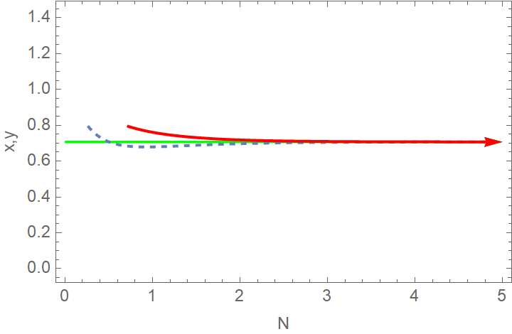
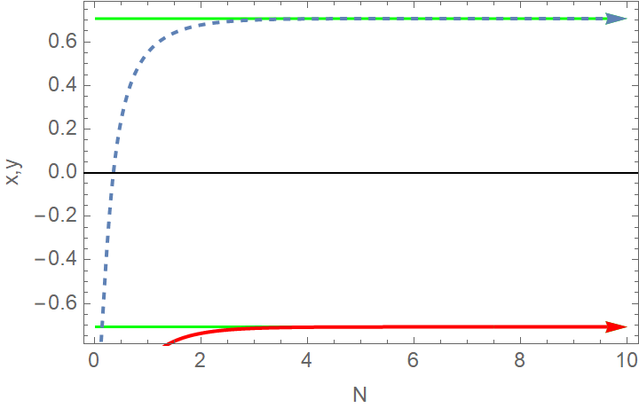
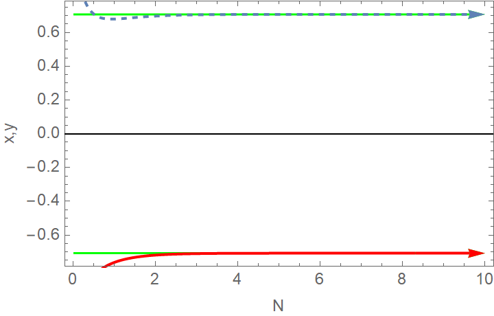
Figure 1: Trajectories $x(N)$ (blue dashed curve) and $y(N)$ (red thick curve) in the phase space of the dynamical system (55) for various initial conditions. The green lines indicate the values $1/\sqrt{2}$ and $-1/\sqrt{2}$. As it can be seen, the stable dark matter attractors $P_{4}^{*}$ and $P_{5}^{*}$ are reached quite fast in the phase space.

In Fig. 2 we present the trajectories of the dynamical system (55) in the $x(N)-y(N)$ plane for various initial conditions. As it can be seen, there exist various trajectories in the phase space but the most interesting for our scenario are the magenta dashed one and the blue thick curves, which both pass through the unstable fixed point $P_{2}^{*}$ before ending to the stable dark matter attractors $P_{4}^{*}$ and $P_{5}^{*}$ respectively.

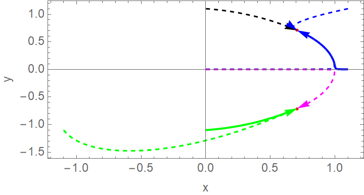
Figure 2: Trajectories in the $x(N)-y(N)$ plane of the phase space of the dynamical system (55) for various initial conditions. Note the magenta dashed and the blue thick curves, which both pass through the unstable fixed point $P_{2}^{*}$ before ending to the stable dark matter attractors $P_{4}^{*}$ and $P_{5}^{*}$ respectively.

Apparently, our theoretical prediction that the dynamical system composed by the matter and scalar field fluids may experience a short stiff evolution after the critical matter density $\rho_{m}^{c}$, during the radiation domination era, before the BBN, is a probably realistic scenario, which may have profound observational implications, regarding gravitational wave physics. This is the subject of the next section.

Let us recapitulate at this point our findings. We initially assumed a non-trivial interaction between the matter-scalar field fluids, which after critical matter density $\rho_{m}^{c}$, reached during the radiation domination era by the dark matter fluid, makes the scalar field fluid to gain energy from the dark matter fluid. Since these two fluids dominate the evolution during the radiation domination era, we studied the two-dimensional phase space formed by these two fluids. We demonstrated that there exist two stable dark matter dominated fixed points, and two unstable kination dominated fixed points, all realized by the scalar field. We analyzed the trajectories in the phase space and we showed that there exist trajectories which pass from the unstable kination fixed point $P_{2}^{*}$ before they end up to the dark matter fixed points. Thus it is possible that the total EoS of the Universe during the radiation domination era might be deformed and can actually be larger than $w=1/3$. This scalar field originating EoS deformations of the radiation domination era may have profound observational implications related to the energy spectrum of the primordial gravitational waves. In the next section we shall analyze this possibility in some detail.

III Radiation Domination EoS Deformations and the Energy Spectrum of the Primordial Gravitational Waves

After the poor findings in the Large Hadron Collider in the post-Higgs discovery, the focus of theoretical physicists has turned to the sky and specifically to CMB related and gravitational waves related experiments. There is a large stream of articles in the literature on primordial gravitational waves, see for example Refs. [123, 124, 125, 126, 127, 128, 129, 130, 131, 77, 132, 133, 134, 135, 136, 137, 138, 139, 140, 141, 142, 143, 144, 145, 146, 147, 148, 149, 150, 151, 152, 153, 154, 155, 156, 157, 158, 159, 160, 161, 162, 163] and the recent review Ref. [164] and references therein. Regarding the energy spectrum of the gravitational waves, taking into account a standard radiation domination era followed by a dark matter era, and the latter followed by a dark energy era, this is equal to,

$$\Omega_{\rm gw}(f)=\frac{k^{2}}{12H_{0}^{2}}\Delta_{h}^{2}(k),$$ (56)

with $\Delta_{h}^{2}(k)$ being equal to,

$$\Delta_{h}^{2}(k)=\Delta_{h}^{({\rm p})}(k)^{2}\left(\frac{\Omega_{m}}{\Omega_{\Lambda}}\right)^{2}\left(\frac{g_{*}(T_{\rm in})}{g_{*0}}\right)\left(\frac{g_{*s0}}{g_{*s}(T_{\rm in})}\right)^{4/3}\left(\overline{\frac{3j_{1}(k\tau_{0})}{k\tau_{0}}}\right)^{2}T_{1}^{2}\left(x_{\rm eq}\right)T_{2}^{2}\left(x_{R}\right)\,,$$ (57)

and the oscillating term must be calculated for a Hubble time, and in addition $\Delta_{h}^{({\rm p})}(k)^{2}$ stands for the primordial tensor power spectrum of the inflationary era, and it is equal to,

$$\Delta_{h}^{({\rm p})}(k)^{2}=\mathcal{A}_{T}(k_{ref})\left(\frac{k}{k_{ref}}\right)^{n_{\mathcal{T}}}\,.$$ (58)

The above must be calculated at the CMB pivot scale which we assume it is $k_{ref}=0.002$ Mpc^-1, and $n_{\mathcal{T}}$ denotes the tensor spectral index, while $\mathcal{A}_{T}(k_{ref})$ stands for amplitude of the tensor perturbations amplitude which can be expressed in terms of the amplitude of the scalar perturbations $\mathcal{P}_{\zeta}(k_{ref})$ in the following way,

$$\mathcal{A}_{T}(k_{ref})=r\mathcal{P}_{\zeta}(k_{ref})\,,$$ (59)

with $r$ being the tensor-to-scalar ratio. Hence,

$$\Delta_{h}^{({\rm p})}(k)^{2}=r\mathcal{P}_{\zeta}(k_{ref})\left(\frac{k}{k_{ref}}\right)^{n_{\mathcal{T}}}\,.$$ (60)

Note that the transfer function $T_{1}(x_{\rm eq})$ in Eq. (57) directly connects the energy spectrum at present day with the modes $k$ which reentered the Hubble horizon during the matter-radiation equality, and this is equal to,

$$T_{1}^{2}(x_{\rm eq})=\left[1+1.57x_{\rm eq}+3.42x_{\rm eq}^{2}\right],$$ (61)

where $x_{\rm eq}=k/k_{\rm eq}$ and $k_{\rm eq}\equiv a(t_{\rm eq})H(t_{\rm eq})=7.1\times 10^{-2}\Omega_{m}h^{2}$ Mpc^-1. Furthermore, the other transfer function $T_{2}(x_{R})$ directly connects the energy spectrum of the gravitational waves at present day to the one corresponding to the era that the mode $k$ reentered the Hubble horizon during the reheating era and before it ended, therefore when $k>k_{R}$, and the transfer function is equal to,

$$T_{2}^{2}\left(x_{R}\right)=\left(1-0.22x^{1.5}+0.65x^{2}\right)^{-1}\,,$$ (62)

with $x_{R}=\frac{k}{k_{R}}$, while the reheating temperature wavenumber $k_{R}$ is equal to,

$$k_{R}\simeq 1.7\times 10^{13}~{}{\rm Mpc^{-1}}\left(\frac{g_{*s}(T_{R})}{106.75}\right)^{1/6}\left(\frac{T_{R}}{10^{6}~{}{\rm GeV}}\right)\,,$$ (63)

where $T_{R}$ stands for the reheating temperature. Note that for the energy spectrum of the gravitational waves at present day we took into account the overall damping effect in the early Universe generated by the non-constancy of the total number of the relativistic degrees of freedom in which case the scale factor behaves as $a(t)\propto T^{-1}$ [165], hence the total damping factor due to this behaves as,

$$\left(\frac{g_{*}(T_{\rm in})}{g_{*0}}\right)\left(\frac{g_{*s0}}{g_{*s}(T_{\rm in})}\right)^{4/3},$$ (64)

with $T_{\rm in}$ denotes the temperature at the horizon reentry,

$$T_{\rm in}\simeq 5.8\times 10^{6}~{}{\rm GeV}\left(\frac{g_{*s}(T_{\rm in})}{106.75}\right)^{-1/6}\left(\frac{k}{10^{14}~{}{\rm Mpc^{-1}}}\right).$$ (65)

Note that the reheating temperature is basically an unknown free parameter in the above context. Furthermore, $g_{*}(T_{\mathrm{in}}(k))$ in Eq. (57) is equal to [166],

$$g_{*}(T_{\mathrm{in}}(k))=g_{*0}\left(\frac{A+\tanh\left[-2.5\log_{10}\left(\frac{k/2\pi}{2.5\times 10^{-12}\mathrm{Hz}}\right)\right]}{A+1}\right)\left(\frac{B+\tanh\left[-2\log_{10}\left(\frac{k/2\pi}{6\times 10^{-19}\mathrm{Hz}}\right)\right]}{B+1}\right)\,,$$ (66)

where $A$ and $B$ are equal to,

$$A=\frac{-1-10.75/g_{*0}}{-1+10.75g_{*0}}\,,$$ (67)

$$B=\frac{-1-g_{max}/10.75}{-1+g_{max}/10.75}\,,$$ (68)

with $g_{max}=106.75$ and $g_{*0}=3.36$. Moreover $g_{*0}(T_{\mathrm{in}}(k))$ can be calculated by simply replacing $g_{*0}=3.36$ with $g_{*s}=3.91$ in Eqs. (66), (67) and (68). As a final comment, for the calculation of the energy spectrum of the primordial gravitational waves, we also took into account the damping factor $\sim(\Omega_{m}/\Omega_{\Lambda})^{2}$ due to the present day acceleration of the Universe.

In the previous section we showed that it is possible for the Universe to experience short deformations of its total EoS parameter during the radiation domination era (can also be during the reheating era). Thus let us see how these pre-BBN deformations can affect the energy spectrum of the primordial gravitational waves. We will assume that the EoS deformations occur when wavenumbers of the order $k_{s}\sim 10^{11}\,$Mpc^-1 reenter the Hubble horizon, so this era corresponds to the reheating era, or at some point during the early radiation domination era. Since the scalar field stiff attractors, affect the total EoS during the reheating, we will assume that the total background EoS parameter during this era is $w=0.8$, or even larger, somewhere in the range $w\sim[1/3,1]$. The change of the background EoS parameter for a dark matter dominated one, to the value $w$, has its imprint on the energy spectrum of the gravitational waves, since an overall multiplication factor of the form $\sim\left(\frac{k}{k_{s}}\right)^{r_{s}}$ is included in the energy spectrum, where $r_{s}=-2\left(\frac{1-3w}{1+3w}\right)$ [90]. Therefore, the final expression for the total $h^{2}$-scaled energy spectrum of the primordial gravitational waves finally takes the form,

$$h^{2}\Omega_{\rm gw}(f)=S_{k}(f)\times\frac{k^{2}}{12H_{0}^{2}}r\mathcal{P}_{\zeta}(k_{ref})\left(\frac{k}{k_{ref}}\right)^{n_{\mathcal{T}}}\left(\frac{\Omega_{m}}{\Omega_{\Lambda}}\right)^{2}\left(\frac{g_{*}(T_{\rm in})}{g_{*0}}\right)\left(\frac{g_{*s0}}{g_{*s}(T_{\rm in})}\right)^{4/3}\left(\overline{\frac{3j_{1}(k\tau_{0})}{k\tau_{0}}}\right)^{2}T_{1}^{2}\left(x_{\rm eq}\right)T_{2}^{2}\left(x_{R}\right)\,,$$

where $S_{k}(f)$,

$$S_{k}(f)=\left(\frac{k}{k_{s}}\right)^{r_{s}}\,,$$ (69)

and recall that $k_{ref}$ is the CMB pivot scale $k_{ref}=0.002$ Mpc^-1 and $n_{\mathcal{T}}$ stands for the tensor spectral index of the primordial tensor perturbations, while $r$ denotes the tensor-to-scalar ratio. It is important to note once more that the reheating temperature is a free variable and as it will prove once more, it will play an important role in the final form of the predicted energy spectrum of the primordial gravitational waves. Having all the necessary information at hand, we now proceed to the determination of the predicted energy spectrum of the primordial gravitational waves.

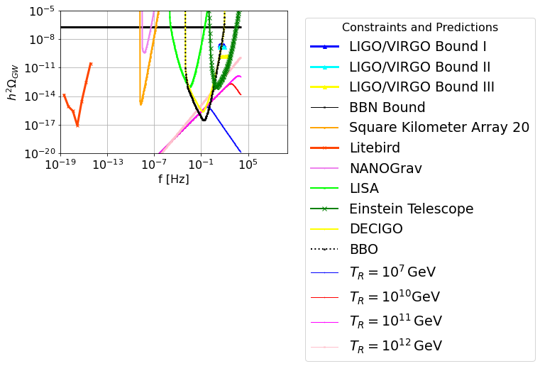
Figure 3: The $h^{2}$-scaled gravitational wave energy spectrum for the $R^{2}$ gravity driven inflationary era and a EoS deformations of the reheating era which make the total EoS parameter take values $w_{tot}>1/3$. We took $w_{tot}=0.8$ which occurs when the modes with wavenumber $k=10^{11}\,$Mpc^-1 reenter the Hubble horizon. The blue curve corresponds to the reheating temperature $T_{R}=10^{7}\,$GeV, the red curve to $T_{R}=10^{10}\,$GeV, the magenta curve to $T_{R}=10^{11}\,$GeV and the pink curve to $T_{R}=10^{12}\,$GeV.

In Fig. 3 we present the $h^{2}$-scaled gravitational wave energy spectrum for the model under study which contains a primordial $R^{2}$ gravity driving the inflationary era and the effects of EoS deformations with $w_{tot}=0.8$, of the reheating (or early radiation domination) era which occurs when the modes with wavenumber $k=10^{11}\,$Mpc^-1 reenter the Hubble horizon, for four reheating temperatures, $T_{R}=10^{7}\,$GeV (blue curve), $T_{R}=10^{10}\,$GeV (red curve), $T_{R}=10^{11}\,$GeV (magenta curve) and $T_{R}=10^{12}\,$GeV (pink curve). For all the plots we used the tensor spectral index and tensor-to-scalar ratio of the $R^{2}$ model which we derived in the previous section. As it can be seen, all the curves can be detected by the future DECIGO, BBO, but only the large reheating temperature curve can be detected by the Einstein telescope. This result is deemed quite important since the energy spectrum of the pure $R^{2}$ gravity cannot be detected by any of the future gravitational wave experiments. Thus we demonstrated that short EoS deformations occurring during the reheating era, can actually yield a detectable gravitational wave energy spectrum.

Concluding Remarks and Discussion

In this work we proposed a theoretical scenario in which the Universe may pass through a brief reheating era deformations well before the BBN era and well beyond the matter-radiation equality. We used a model which is composed by an $F(R)$ gravity, the radiation perfect fluid and an interacting system of dark matter and scalar field fluids. The model is constructed in such a way so that primordially and at late times the $F(R)$ gravity dominates the evolution, thus producing the inflationary era and the dark energy era, while in between, the Universe is dominated initially by the radiation fluid and eventually after a critical matter density $\rho_{m}^{c}$ during the reheating era or early radiation domination era, by the interacting dark matter and scalar field fluids which dominate over the radiation fluid, or cause disturbance in its dominance over the evolution of the Universe. The interaction between the dark matter and scalar fluids acts in such a way so that after inflation, the scalar field fluid loses its energy and transfers it to the dark matter fluid, and at the critical matter density $\rho_{m}^{c}$ the interaction is switched of effectively, while after the critical matter density $\rho_{m}^{c}$, the interaction flips its sign and the scalar field gains energy from the dark matter fluid. We formed the two-dimensional subspace of the total cosmological phase space, composed by the dark matter and scalar field fluids, and we constructed the autonomous dynamical system that governs this phase space. We calculated the fixed points and as we showed, there exist two unstable stiff fixed points and two stable dark matter attractors. As we showed numerically, there exist initial conditions for which the trajectories in the phase space may pass through one of the two kination fixed points, before ending up to the stable dark matter attractors. This behavior makes possible for the Universe to experience short deformations of its total EoS parameter, and we examined the effects of such a short eras on the energy spectrum of the primordial gravitational waves. As we showed, even with a standard $R^{2}$ inflationary era, the predicted energy spectrum can be detected by the future DECIGO and BBO experiments and in some cases by the Einstein Telescope.

References

- [1] A. D. Linde, Lect. Notes Phys. 738 (2008) 1 [arXiv:0705.0164 [hep-th]].
- [2] D. S. Gorbunov and V. A. Rubakov, “Introduction to the theory of the early universe: Cosmological perturbations and inflationary theory,” Hackensack, USA: World Scientific (2011) 489 p;
- [3] A. Linde, arXiv:1402.0526 [hep-th];
- [4] D. H. Lyth and A. Riotto, Phys. Rept. 314 (1999) 1 [hep-ph/9807278].
- [5] K. N. Abazajian et al. [CMB-S4], [arXiv:1610.02743 [astro-ph.CO]].
- [6] M. H. Abitbol et al. [Simons Observatory], Bull. Am. Astron. Soc. 51 (2019), 147 [arXiv:1907.08284 [astro-ph.IM]].
- [7] S. Hild, M. Abernathy, F. Acernese, P. Amaro-Seoane, N. Andersson, K. Arun, F. Barone, B. Barr, M. Barsuglia and M. Beker, et al. Class. Quant. Grav. 28 (2011), 094013 doi:10.1088/0264-9381/28/9/094013 [arXiv:1012.0908 [gr-qc]].
- [8] J. Baker, J. Bellovary, P. L. Bender, E. Berti, R. Caldwell, J. Camp, J. W. Conklin, N. Cornish, C. Cutler and R. DeRosa, et al. [arXiv:1907.06482 [astro-ph.IM]].
- [9] T. L. Smith and R. Caldwell, Phys. Rev. D 100 (2019) no.10, 104055 doi:10.1103/PhysRevD.100.104055 [arXiv:1908.00546 [astro-ph.CO]].
- [10] J. Crowder and N. J. Cornish, Phys. Rev. D 72 (2005), 083005 doi:10.1103/PhysRevD.72.083005 [arXiv:gr-qc/0506015 [gr-qc]].
- [11] T. L. Smith and R. Caldwell, Phys. Rev. D 95 (2017) no.4, 044036 doi:10.1103/PhysRevD.95.044036 [arXiv:1609.05901 [gr-qc]].
- [12] N. Seto, S. Kawamura and T. Nakamura, Phys. Rev. Lett. 87 (2001), 221103 doi:10.1103/PhysRevLett.87.221103 [arXiv:astro-ph/0108011 [astro-ph]].
- [13] S. Kawamura, M. Ando, N. Seto, S. Sato, M. Musha, I. Kawano, J. Yokoyama, T. Tanaka, K. Ioka and T. Akutsu, et al. [arXiv:2006.13545 [gr-qc]].
- [14] A. Weltman, P. Bull, S. Camera, K. Kelley, H. Padmanabhan, J. Pritchard, A. Raccanelli, S. Riemer-Sørensen, L. Shao and S. Andrianomena, et al. Publ. Astron. Soc. Austral. 37 (2020), e002 doi:10.1017/pasa.2019.42 [arXiv:1810.02680 [astro-ph.CO]].
- [15] P. Auclair et al. [LISA Cosmology Working Group], [arXiv:2204.05434 [astro-ph.CO]].
- [16] G. Agazie et al. [NANOGrav], doi:10.3847/2041-8213/acdac6 [arXiv:2306.16213 [astro-ph.HE]].
- [17] J. Antoniadis, P. Arumugam, S. Arumugam, S. Babak, M. Bagchi, A. S. B. Nielsen, C. G. Bassa, A. Bathula, A. Berthereau and M. Bonetti, et al. [arXiv:2306.16214 [astro-ph.HE]].
- [18] D. J. Reardon, A. Zic, R. M. Shannon, G. B. Hobbs, M. Bailes, V. Di Marco, A. Kapur, A. F. Rogers, E. Thrane and J. Askew, et al. doi:10.3847/2041-8213/acdd02 [arXiv:2306.16215 [astro-ph.HE]].
- [19] H. Xu, S. Chen, Y. Guo, J. Jiang, B. Wang, J. Xu, Z. Xue, R. N. Caballero, J. Yuan and Y. Xu, et al. doi:10.1088/1674-4527/acdfa5 [arXiv:2306.16216 [astro-ph.HE]].
- [20] S. Vagnozzi, JHEAp 39 (2023), 81-98 doi:10.1016/j.jheap.2023.07.001 [arXiv:2306.16912 [astro-ph.CO]].
- [21] V. K. Oikonomou, Phys. Rev. D 108 (2023) no.4, 043516 doi:10.1103/PhysRevD.108.043516 [arXiv:2306.17351 [astro-ph.CO]].
- [22] Y. F. Cai, X. C. He, X. Ma, S. F. Yan and G. W. Yuan, [arXiv:2306.17822 [gr-qc]].
- [23] C. Han, K. P. Xie, J. M. Yang and M. Zhang, [arXiv:2306.16966 [hep-ph]].
- [24] S. Y. Guo, M. Khlopov, X. Liu, L. Wu, Y. Wu and B. Zhu, [arXiv:2306.17022 [hep-ph]].
- [25] J. Yang, N. Xie and F. P. Huang, [arXiv:2306.17113 [hep-ph]].
- [26] A. Addazi, Y. F. Cai, A. Marciano and L. Visinelli, [arXiv:2306.17205 [astro-ph.CO]].
- [27] S. P. Li and K. P. Xie, Phys. Rev. D 108 (2023) no.5, 055018 doi:10.1103/PhysRevD.108.055018 [arXiv:2307.01086 [hep-ph]].
- [28] X. Niu and M. H. Rahat, [arXiv:2307.01192 [hep-ph]].
- [29] A. Yang, J. Ma, S. Jiang and F. P. Huang, [arXiv:2306.17827 [hep-ph]].
- [30] S. Datta, [arXiv:2307.00646 [hep-ph]].
- [31] X. K. Du, M. X. Huang, F. Wang and Y. K. Zhang, [arXiv:2307.02938 [hep-ph]].
- [32] A. Salvio, [arXiv:2307.04694 [hep-ph]].
- [33] Z. Yi, Q. Gao, Y. Gong, Y. Wang and F. Zhang, [arXiv:2307.02467 [gr-qc]].
- [34] Z. Q. You, Z. Yi and Y. Wu, [arXiv:2307.04419 [gr-qc]].
- [35] S. Wang and Z. C. Zhao, [arXiv:2307.04680 [astro-ph.HE]].
- [36] D. G. Figueroa, M. Pieroni, A. Ricciardone and P. Simakachorn, [arXiv:2307.02399 [astro-ph.CO]].
- [37] S. Choudhury, [arXiv:2307.03249 [astro-ph.CO]].
- [38] S. A. Hosseini Mansoori, F. Felegray, A. Talebian and M. Sami, [arXiv:2307.06757 [astro-ph.CO]].
- [39] S. Ge, [arXiv:2307.08185 [gr-qc]].
- [40] L. Bian, S. Ge, J. Shu, B. Wang, X. Y. Yang and J. Zong, [arXiv:2307.02376 [astro-ph.HE]].
- [41] M. Kawasaki and K. Murai, [arXiv:2308.13134 [astro-ph.CO]].
- [42] Z. Yi, Z. Q. You and Y. Wu, [arXiv:2308.05632 [astro-ph.CO]].
- [43] H. An, B. Su, H. Tai, L. T. Wang and C. Yang, [arXiv:2308.00070 [astro-ph.CO]].
- [44] Z. Zhang, C. Cai, Y. H. Su, S. Wang, Z. H. Yu and H. H. Zhang, [arXiv:2307.11495 [hep-ph]].
- [45] P. Di Bari and M. H. Rahat, [arXiv:2307.03184 [hep-ph]].
- [46] S. Jiang, A. Yang, J. Ma and F. P. Huang, [arXiv:2306.17827 [hep-ph]].
- [47] G. Bhattacharya, S. Choudhury, K. Dey, S. Ghosh, A. Karde and N. S. Mishra, [arXiv:2309.00973 [astro-ph.CO]].
- [48] S. Choudhury, A. Karde, S. Panda and M. Sami, [arXiv:2308.09273 [astro-ph.CO]].
- [49] T. Bringmann, P. F. Depta, T. Konstandin, K. Schmidt-Hoberg and C. Tasillo, [arXiv:2306.09411 [astro-ph.CO]].
- [50] S. Choudhury, S. Panda and M. Sami, JCAP 08 (2023), 078 doi:10.1088/1475-7516/2023/08/078 [arXiv:2304.04065 [astro-ph.CO]].
- [51] S. Choudhury, A. Karde, S. Panda and M. Sami, [arXiv:2306.12334 [astro-ph.CO]].
- [52] H. L. Huang, Y. Cai, J. Q. Jiang, J. Zhang and Y. S. Piao, [arXiv:2306.17577 [gr-qc]].
- [53] J. Q. Jiang, Y. Cai, G. Ye and Y. S. Piao, [arXiv:2307.15547 [astro-ph.CO]].
- [54] M. Zhu, G. Ye and Y. Cai, [arXiv:2307.16211 [astro-ph.CO]].
- [55] I. Ben-Dayan, U. Kumar, U. Thattarampilly and A. Verma, [arXiv:2307.15123 [astro-ph.CO]].
- [56] G. Franciolini, A. Iovino, Junior., V. Vaskonen and H. Veermae, [arXiv:2306.17149 [astro-ph.CO]].
- [57] J. Ellis, M. Fairbairn, G. Franciolini, G. Hütsi, A. Iovino, M. Lewicki, M. Raidal, J. Urrutia, V. Vaskonen and H. Veermäe, [arXiv:2308.08546 [astro-ph.CO]].
- [58] L. Liu, Z. C. Chen and Q. G. Huang, [arXiv:2307.01102 [astro-ph.CO]].
- [59] L. Liu, Z. C. Chen and Q. G. Huang, [arXiv:2307.14911 [astro-ph.CO]].
- [60] E. Madge, E. Morgante, C. Puchades-Ibáñez, N. Ramberg, W. Ratzinger, S. Schenk and P. Schwaller, [arXiv:2306.14856 [hep-ph]].
- [61] M. X. Huang, F. Wang and Y. K. Zhang, [arXiv:2309.06378 [hep-ph]].
- [62] C. Fu, J. Liu, X. Y. Yang, W. W. Yu and Y. Zhang, [arXiv:2308.15329 [astro-ph.CO]].
- [63] R. Maji and W. I. Park, [arXiv:2308.11439 [hep-ph]].
- [64] M. R. Gangopadhyay, V. V. Godithi, K. Ichiki, R. Inui, T. Kajino, A. Manusankar, G. J. Mathews and Yogesh, [arXiv:2309.03101 [astro-ph.CO]].
- [65] S. Wang, Z. C. Zhao and Q. H. Zhu, [arXiv:2307.03095 [astro-ph.CO]].
- [66] S. Wang, Z. C. Zhao, J. P. Li and Q. H. Zhu, [arXiv:2307.00572 [astro-ph.CO]].
- [67] P. Schwaller, Phys. Rev. Lett. 115 (2015) no.18, 181101 doi:10.1103/PhysRevLett.115.181101 [arXiv:1504.07263 [hep-ph]].
- [68] W. Ratzinger and P. Schwaller, SciPost Phys. 10 (2021) no.2, 047 doi:10.21468/SciPostPhys.10.2.047 [arXiv:2009.11875 [astro-ph.CO]].
- [69] A. Ashoorioon, K. Rezazadeh and A. Rostami, Phys. Lett. B 835 (2022), 137542 doi:10.1016/j.physletb.2022.137542 [arXiv:2202.01131 [astro-ph.CO]].
- [70] S. Choudhury, M. R. Gangopadhyay and M. Sami, [arXiv:2301.10000 [astro-ph.CO]].
- [71] S. Choudhury, S. Panda and M. Sami, [arXiv:2302.05655 [astro-ph.CO]].
- [72] S. Choudhury, S. Panda and M. Sami, [arXiv:2303.06066 [astro-ph.CO]].
- [73] L. Bian, S. Ge, C. Li, J. Shu and J. Zong, [arXiv:2212.07871 [hep-ph]].
- [74] C. S. Machado, W. Ratzinger, P. Schwaller and B. A. Stefanek, JHEP 01 (2019), 053 doi:10.1007/JHEP01(2019)053 [arXiv:1811.01950 [hep-ph]].
- [75] T. Regimbau, Symmetry 14 (2022) no.2, 270 doi:10.3390/sym14020270
- [76] M. Benetti, L. L. Graef and S. Vagnozzi, Phys. Rev. D 105 (2022) no.4, 043520 doi:10.1103/PhysRevD.105.043520 [arXiv:2111.04758 [astro-ph.CO]].
- [77] S. Vagnozzi, Mon. Not. Roy. Astron. Soc. 502 (2021) no.1, L11-L15 doi:10.1093/mnrasl/slaa203 [arXiv:2009.13432 [astro-ph.CO]].
- [78] V. Kamali and R. Brandenberger, Phys. Rev. D 101 (2020) no.10, 103512 doi:10.1103/PhysRevD.101.103512 [arXiv:2002.09771 [hep-th]].
- [79] R. H. Brandenberger, Class. Quant. Grav. 32 (2015) no.23, 234002 doi:10.1088/0264-9381/32/23/234002 [arXiv:1505.02381 [hep-th]].
- [80] R. H. Brandenberger, S. Kanno, J. Soda, D. A. Easson, J. Khoury, P. Martineau, A. Nayeri and S. P. Patil, JCAP 11 (2006), 009 doi:10.1088/1475-7516/2006/11/009 [arXiv:hep-th/0608186 [hep-th]].
- [81] A. Ashtekar and P. Singh, Class. Quant. Grav. 28 (2011), 213001 doi:10.1088/0264-9381/28/21/213001 [arXiv:1108.0893 [gr-qc]].
- [82] M. Bojowald, G. Calcagni and S. Tsujikawa, JCAP 11 (2011), 046 doi:10.1088/1475-7516/2011/11/046 [arXiv:1107.1540 [gr-qc]].
- [83] J. Mielczarek, Phys. Rev. D 79 (2009), 123520 doi:10.1103/PhysRevD.79.123520 [arXiv:0902.2490 [gr-qc]].
- [84] M. Bojowald, Class. Quant. Grav. 26 (2009), 075020 doi:10.1088/0264-9381/26/7/075020 [arXiv:0811.4129 [gr-qc]].
- [85] G. Calcagni and S. Kuroyanagi, JCAP 03 (2021), 019 doi:10.1088/1475-7516/2021/03/019 [arXiv:2012.00170 [gr-qc]].
- [86] A. S. Koshelev, K. Sravan Kumar, A. Mazumdar and A. A. Starobinsky, JHEP 06 (2020), 152 doi:10.1007/JHEP06(2020)152 [arXiv:2003.00629 [hep-th]].
- [87] A. S. Koshelev, K. Sravan Kumar and A. A. Starobinsky, JHEP 03 (2018), 071 doi:10.1007/JHEP03(2018)071 [arXiv:1711.08864 [hep-th]].
- [88] M. Baumgart, J. J. Heckman and L. Thomas, JCAP 07 (2022) no.07, 034 doi:10.1088/1475-7516/2022/07/034 [arXiv:2109.08166 [hep-ph]].
- [89] R. T. Co, D. Dunsky, N. Fernandez, A. Ghalsasi, L. J. Hall, K. Harigaya and J. Shelton, JHEP 09 (2022), 116 doi:10.1007/JHEP09(2022)116 [arXiv:2108.09299 [hep-ph]].
- [90] Y. Gouttenoire, G. Servant and P. Simakachorn, [arXiv:2111.01150 [hep-ph]].
- [91] M. Giovannini, Phys. Rev. D 58 (1998), 083504 doi:10.1103/PhysRevD.58.083504 [arXiv:hep-ph/9806329 [hep-ph]].
- [92] V. K. Oikonomou, Phys. Rev. D 107 (2023) no.6, 064071 doi:10.1103/PhysRevD.107.064071 [arXiv:2303.05889 [hep-ph]].
- [93] L. H. Ford, Phys. Rev. D 35 (1987), 2955 doi:10.1103/PhysRevD.35.2955
- [94] M. Kamionkowski and M. S. Turner, Phys. Rev. D 42 (1990), 3310-3320 doi:10.1103/PhysRevD.42.3310
- [95] D. Grin, T. L. Smith and M. Kamionkowski, Phys. Rev. D 77 (2008), 085020 doi:10.1103/PhysRevD.77.085020 [arXiv:0711.1352 [astro-ph]].
- [96] L. Visinelli and P. Gondolo, Phys. Rev. D 81 (2010), 063508 doi:10.1103/PhysRevD.81.063508 [arXiv:0912.0015 [astro-ph.CO]].
- [97] M. Giovannini, Class. Quant. Grav. 16 (1999), 2905-2913 doi:10.1088/0264-9381/16/9/308 [arXiv:hep-ph/9903263 [hep-ph]].
- [98] M. Giovannini, Phys. Rev. D 60 (1999), 123511 doi:10.1103/PhysRevD.60.123511 [arXiv:astro-ph/9903004 [astro-ph]].
- [99] K. Harigaya, K. Inomata and T. Terada, [arXiv:2309.00228 [astro-ph.CO]].
- [100] S. Nojiri, S. D. Odintsov and V. K. Oikonomou, Phys. Rept. 692 (2017) 1 [arXiv:1705.11098 [gr-qc]].
-
[101]
S. Capozziello, M. De Laurentis,
Phys. Rept. 509, 167 (2011);
V. Faraoni and S. Capozziello, Fundam. Theor. Phys. 170 (2010). - [102] S. Nojiri, S.D. Odintsov, eConf C0602061, 06 (2006) [Int. J. Geom. Meth. Mod. Phys. 4, 115 (2007)].
- [103] S. Nojiri, S.D. Odintsov, Phys. Rept. 505, 59 (2011);
- [104] G. J. Olmo, Int. J. Mod. Phys. D 20 (2011) 413 [arXiv:1101.3864 [gr-qc]].
- [105] L. Sebastiani, S. Vagnozzi and R. Myrzakulov, Adv. High Energy Phys. 2017 (2017), 3156915 doi:10.1155/2017/3156915 [arXiv:1612.08661 [gr-qc]].
- [106] S. D. Odintsov, V. K. Oikonomou, I. Giannakoudi, F. P. Fronimos and E. C. Lymperiadou, [arXiv:2307.16308 [gr-qc]].
- [107] E. J. Copeland, A. R. Liddle and D. Wands, Phys. Rev. D 57 (1998), 4686-4690 doi:10.1103/PhysRevD.57.4686 [arXiv:gr-qc/9711068 [gr-qc]].
- [108] C. G. Boehmer, G. Caldera-Cabral, R. Lazkoz and R. Maartens, Phys. Rev. D 78 (2008), 023505 doi:10.1103/PhysRevD.78.023505 [arXiv:0801.1565 [gr-qc]].
- [109] W. Yang, S. Pan, O. Mena and E. Di Valentino, JHEAp 40 (2023), 19-40 doi:10.1016/j.jheap.2023.09.001 [arXiv:2209.14816 [astro-ph.CO]].
- [110] R. C. Nunes, S. Vagnozzi, S. Kumar, E. Di Valentino and O. Mena, Phys. Rev. D 105 (2022) no.12, 123506 doi:10.1103/PhysRevD.105.123506 [arXiv:2203.08093 [astro-ph.CO]].
- [111] S. Gariazzo, E. Di Valentino, O. Mena and R. C. Nunes, Phys. Rev. D 106 (2022) no.2, 023530 doi:10.1103/PhysRevD.106.023530 [arXiv:2111.03152 [astro-ph.CO]].
- [112] R. C. Nunes and E. Di Valentino, Phys. Rev. D 104 (2021) no.6, 063529 doi:10.1103/PhysRevD.104.063529 [arXiv:2107.09151 [astro-ph.CO]].
- [113] W. Yang, E. Di Valentino, S. Pan, Y. Wu and J. Lu, Mon. Not. Roy. Astron. Soc. 501 (2021) no.4, 5845-5858 doi:10.1093/mnras/staa3914 [arXiv:2101.02168 [astro-ph.CO]].
- [114] W. Yang, O. Mena, S. Pan and E. Di Valentino, Phys. Rev. D 100 (2019) no.8, 083509 doi:10.1103/PhysRevD.100.083509 [arXiv:1906.11697 [astro-ph.CO]].
- [115] W. Yang, S. Pan, E. Di Valentino, A. Paliathanasis and J. Lu, Phys. Rev. D 100 (2019) no.10, 103518 doi:10.1103/PhysRevD.100.103518 [arXiv:1906.04162 [astro-ph.CO]].
- [116] W. Yang, A. Mukherjee, E. Di Valentino and S. Pan, Phys. Rev. D 98 (2018) no.12, 123527 doi:10.1103/PhysRevD.98.123527 [arXiv:1809.06883 [astro-ph.CO]].
- [117] S. A. Appleby, R. A. Battye and A. A. Starobinsky, JCAP 06 (2010), 005 doi:10.1088/1475-7516/2010/06/005 [arXiv:0909.1737 [astro-ph.CO]].
- [118] C. Wetterich, Astron. Astrophys. 301 (1995), 321-328 [arXiv:hep-th/9408025 [hep-th]].
- [119] N. Aghanim et al. [Planck], Astron. Astrophys. 641 (2020), A6 [erratum: Astron. Astrophys. 652 (2021), C4] doi:10.1051/0004-6361/201833910 [arXiv:1807.06209 [astro-ph.CO]].
- [120] V. K. Oikonomou, Phys. Rev. D 103 (2021) no.12, 124028 doi:10.1103/PhysRevD.103.124028 [arXiv:2012.01312 [gr-qc]].
- [121] J. c. Hwang and H. Noh, Phys. Rev. D 71 (2005), 063536 doi:10.1103/PhysRevD.71.063536 [arXiv:gr-qc/0412126 [gr-qc]].
- [122] S. D. Odintsov and V. K. Oikonomou, Phys. Lett. B 807 (2020), 135576 doi:10.1016/j.physletb.2020.135576 [arXiv:2005.12804 [gr-qc]].
- [123] M. Kamionkowski and E. D. Kovetz, Ann. Rev. Astron. Astrophys. 54 (2016), 227-269 doi:10.1146/annurev-astro-081915-023433 [arXiv:1510.06042 [astro-ph.CO]].
- [124] M. S. Turner, M. J. White and J. E. Lidsey, Phys. Rev. D 48 (1993), 4613-4622 doi:10.1103/PhysRevD.48.4613 [arXiv:astro-ph/9306029 [astro-ph]].
- [125] L. A. Boyle and P. J. Steinhardt, Phys. Rev. D 77 (2008), 063504 doi:10.1103/PhysRevD.77.063504 [arXiv:astro-ph/0512014 [astro-ph]].
- [126] Y. Zhang, Y. Yuan, W. Zhao and Y. T. Chen, Class. Quant. Grav. 22 (2005), 1383-1394 doi:10.1088/0264-9381/22/7/011 [arXiv:astro-ph/0501329 [astro-ph]].
- [127] C. Caprini and D. G. Figueroa, Class. Quant. Grav. 35 (2018) no.16, 163001 doi:10.1088/1361-6382/aac608 [arXiv:1801.04268 [astro-ph.CO]].
- [128] T. J. Clarke, E. J. Copeland and A. Moss, JCAP 10 (2020), 002 doi:10.1088/1475-7516/2020/10/002 [arXiv:2004.11396 [astro-ph.CO]].
- [129] T. L. Smith, M. Kamionkowski and A. Cooray, Phys. Rev. D 73 (2006), 023504 doi:10.1103/PhysRevD.73.023504 [arXiv:astro-ph/0506422 [astro-ph]].
- [130] M. Giovannini, Class. Quant. Grav. 26 (2009), 045004 doi:10.1088/0264-9381/26/4/045004 [arXiv:0807.4317 [astro-ph]].
- [131] X. J. Liu, W. Zhao, Y. Zhang and Z. H. Zhu, Phys. Rev. D 93 (2016) no.2, 024031 doi:10.1103/PhysRevD.93.024031 [arXiv:1509.03524 [astro-ph.CO]].
- [132] M. Giovannini, [arXiv:2303.11928 [gr-qc]].
- [133] M. Giovannini, Eur. Phys. J. C 82 (2022) no.9, 828 doi:10.1140/epjc/s10052-022-10800-4 [arXiv:2206.08217 [gr-qc]].
- [134] M. Giovannini, Phys. Rev. D 105 (2022) no.10, 103524 doi:10.1103/PhysRevD.105.103524 [arXiv:2203.13586 [gr-qc]].
- [135] M. Giovannini, Phys. Lett. B 810 (2020), 135801 doi:10.1016/j.physletb.2020.135801 [arXiv:2006.02760 [gr-qc]].
- [136] M. Giovannini, Prog. Part. Nucl. Phys. 112 (2020), 103774 doi:10.1016/j.ppnp.2020.103774 [arXiv:1912.07065 [astro-ph.CO]].
- [137] M. Giovannini, Phys. Rev. D 100 (2019) no.8, 083531 doi:10.1103/PhysRevD.100.083531 [arXiv:1908.09679 [hep-th]].
- [138] M. Giovannini, Phys. Rev. D 91 (2015) no.2, 023521 doi:10.1103/PhysRevD.91.023521 [arXiv:1410.5307 [hep-th]].
- [139] M. Giovannini, PMC Phys. A 4 (2010), 1 doi:10.1186/1754-0410-4-1 [arXiv:0901.3026 [astro-ph.CO]].
- [140] M. Kamionkowski, A. Kosowsky and M. S. Turner, Phys. Rev. D 49 (1994), 2837-2851 doi:10.1103/PhysRevD.49.2837 [arXiv:astro-ph/9310044 [astro-ph]].
- [141] W. Giarè and F. Renzi, Phys. Rev. D 102 (2020) no.8, 083530 doi:10.1103/PhysRevD.102.083530 [arXiv:2007.04256 [astro-ph.CO]].
- [142] W. Zhao and Y. Zhang, Phys. Rev. D 74 (2006), 043503 doi:10.1103/PhysRevD.74.043503 [arXiv:astro-ph/0604458 [astro-ph]].
- [143] P. D. Lasky, C. M. F. Mingarelli, T. L. Smith, J. T. Giblin, D. J. Reardon, R. Caldwell, M. Bailes, N. D. R. Bhat, S. Burke-Spolaor and W. Coles, et al. Phys. Rev. X 6 (2016) no.1, 011035 doi:10.1103/PhysRevX.6.011035 [arXiv:1511.05994 [astro-ph.CO]].
- [144] R. G. Cai, C. Fu and W. W. Yu, [arXiv:2112.04794 [astro-ph.CO]].
- [145] S. D. Odintsov, V. K. Oikonomou and F. P. Fronimos, Phys. Dark Univ. 35 (2022), 100950 doi:10.1016/j.dark.2022.100950 [arXiv:2108.11231 [gr-qc]].
- [146] J. Lin, S. Gao, Y. Gong, Y. Lu, Z. Wang and F. Zhang, [arXiv:2111.01362 [gr-qc]].
- [147] F. Zhang, J. Lin and Y. Lu, Phys. Rev. D 104 (2021) no.6, 063515 [erratum: Phys. Rev. D 104 (2021) no.12, 129902] doi:10.1103/PhysRevD.104.063515 [arXiv:2106.10792 [gr-qc]].
- [148] L. Visinelli, N. Bolis and S. Vagnozzi, Phys. Rev. D 97 (2018) no.6, 064039 doi:10.1103/PhysRevD.97.064039 [arXiv:1711.06628 [gr-qc]].
- [149] J. R. Pritchard and M. Kamionkowski, Annals Phys. 318 (2005), 2-36 doi:10.1016/j.aop.2005.03.005 [arXiv:astro-ph/0412581 [astro-ph]].
- [150] V. V. Khoze and D. L. Milne, [arXiv:2212.04784 [hep-ph]].
- [151] A. Casalino, M. Rinaldi, L. Sebastiani and S. Vagnozzi, Phys. Dark Univ. 22 (2018), 108 doi:10.1016/j.dark.2018.10.001 [arXiv:1803.02620 [gr-qc]].
- [152] V. K. Oikonomou, Astropart. Phys. 141 (2022), 102718 doi:10.1016/j.astropartphys.2022.102718 [arXiv:2204.06304 [gr-qc]].
- [153] A. Casalino, M. Rinaldi, L. Sebastiani and S. Vagnozzi, Class. Quant. Grav. 36 (2019) no.1, 017001 doi:10.1088/1361-6382/aaf1fd [arXiv:1811.06830 [gr-qc]].
- [154] K. El Bourakadi, B. Asfour, Z. Sakhi, Z. M. Bennai and T. Ouali, Eur. Phys. J. C 82 (2022) no.9, 792 doi:10.1140/epjc/s10052-022-10762-7 [arXiv:2209.08585 [gr-qc]].
- [155] R. Sturani, Symmetry 13 (2021) no.12, 2384 doi:10.3390/sym13122384
- [156] S. Vagnozzi and A. Loeb, Astrophys. J. Lett. 939 (2022) no.2, L22 doi:10.3847/2041-8213/ac9b0e [arXiv:2208.14088 [astro-ph.CO]].
- [157] A. S. Arapoğlu and A. E. Yükselci, [arXiv:2210.16699 [gr-qc]].
- [158] W. Giarè, M. Forconi, E. Di Valentino and A. Melchiorri, [arXiv:2210.14159 [astro-ph.CO]].
- [159] V. K. Oikonomou, Class. Quant. Grav. 38 (2021) no.19, 195025 doi:10.1088/1361-6382/ac2168 [arXiv:2108.10460 [gr-qc]].
- [160] M. Gerbino, K. Freese, S. Vagnozzi, M. Lattanzi, O. Mena, E. Giusarma and S. Ho, Phys. Rev. D 95 (2017) no.4, 043512 doi:10.1103/PhysRevD.95.043512 [arXiv:1610.08830 [astro-ph.CO]].
- [161] M. Breitbach, J. Kopp, E. Madge, T. Opferkuch and P. Schwaller, JCAP 07 (2019), 007 doi:10.1088/1475-7516/2019/07/007 [arXiv:1811.11175 [hep-ph]].
- [162] S. Pi, M. Sasaki and Y. l. Zhang, JCAP 06 (2019), 049 doi:10.1088/1475-7516/2019/06/049 [arXiv:1904.06304 [gr-qc]].
- [163] M. Khlopov and S. R. Chowdhury, Symmetry 15 (2023) no.4, 832 doi:10.3390/sym15040832
- [164] S. D. Odintsov, V. K. Oikonomou and R. Myrzakulov, Symmetry 14 (2022) no.4, 729 doi:10.3390/sym14040729 [arXiv:2204.00876 [gr-qc]].
- [165] Y. Watanabe and E. Komatsu, Phys. Rev. D 73 (2006), 123515 doi:10.1103/PhysRevD.73.123515 [arXiv:astro-ph/0604176 [astro-ph]].
- [166] S. Kuroyanagi, T. Takahashi and S. Yokoyama, JCAP 02 (2015), 003 doi:10.1088/1475-7516/2015/02/003 [arXiv:1407.4785 [astro-ph.CO]].
- [167] M. Kamionkowski and A. G. Riess, [arXiv:2211.04492 [astro-ph.CO]].