Fair Data Generation via Score-based Diffusion Model

Abstract.

The fairness of AI decision-making has garnered increasing attention, leading to the proposal of numerous fairness algorithms. In this paper, we aim not to address this issue by directly introducing fair learning algorithms, but rather by generating entirely new, fair synthetic data from biased datasets for use in any downstream tasks. Additionally, the distribution of test data may differ from that of the training set, potentially impacting the performance of the generated synthetic data in downstream tasks. To address these two challenges, we propose a diffusion model-based framework, FADM: Fairness-Aware Diffusion with Meta-learning. FADM introduces two types of gradient induction during the sampling phase of the diffusion model: one to ensure that the generated samples belong to the desired target categories, and another to make the sensitive attributes of the generated samples difficult to classify into any specific sensitive attribute category. To overcome data distribution shifts in the test environment, we train the diffusion model and the two classifiers used for induction within a meta-learning framework. Compared to other baselines, FADM allows for flexible control over the categories of the generated samples and exhibits superior generalization capability. Experiments on real datasets demonstrate that FADM achieves better accuracy and optimal fairness in downstream tasks.

1. Introduction

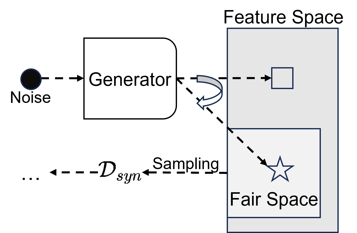
Figure 1. An illustration of the fair generation task. The generated samples are produced from noise and are distinct individuals from those used to train the generator. Through certain inductions, the generated samples are concentrated in a subspace of the feature space that does not contain sensitive information (referred to as the fair space). The dataset $\mathcal{D}_{syn}$ sampled from the fair space can be utilized for training various downstream tasks.

Fairness in machine learning is a critical aspect of the ethical deployment of automated systems, aiming to ensure that these systems do not perpetuate or amplify existing biases and inequalities. A sensitive feature is defined as an attribute that contains protected information about individuals or groups within a dataset. This information may encompass characteristics such as race, gender, religion, or socioeconomic status, which are safeguarded by ethical considerations, legal regulations, or societal norms (Caton and Haas, 2024). Machine learning models have the potential to inadvertently acquire discriminatory patterns if sensitive variables exhibit spurious correlations with the target variable or predictive outcomes (Pessach and Shmueli, 2022; Oneto and Chiappa, 2020). The field has gained significant attention due to the widespread use of machine learning in sensitive areas such as hiring, criminal justice, and lending, where biased outcomes can have severe societal implications.

Currently, numerous methods focus on removing sensitive information from the original dataset to train a fair model (Zemel et al., 2013; Deka and Sutherland, 2023). Unlike these approaches, the objective of this paper is to generate fair data (Fig.1). Specifically, the aim is to produce fair data from input noise while ensuring the quality of the data. Being able to generate fair data is important because end-users creating models based on publicly available data might be unaware they are inadvertently including bias or insufficiently knowledgeable to remove it from their model (Van Breugel et al., 2021). A synthetically generated fair dataset can be applied for training any downstream task, rather than being tailored to a specific model. However, the test-set distribution commonly differs from the training distribution. This will let models encounter surprising failures if there is a significant difference in such distributions (Lin et al., 2023b). A common approach is to decouple environment-independent semantic information. However, for the data generation task, this not only increases the model’s complexity but also makes all subsequent generation processes highly dependent on the completeness of the disentanglement. Therefore, we propose training a diffusion model and two classifiers for guiding sample generation within a meta-learning framework. One classifier guides the generation of samples with specified categories, while the other sensitive attribute classifier ensures the generation of samples devoid of sensitive information. Through meta-training, the diffusion model achieves robust generation capabilities across different domains, and both classifiers maintain accurate classification in various domains, thereby effectively guiding the diffusion model in the correct generation process. Our contributions can be summarized as follows:

• We formulated a new problem: generating unbiased data to train downstream classifiers that are tested on distribution-shifted datasets, while ensuring both accuracy and fairness.

• We have designed a novel fair data generation method called FADM. FADM not only allows for the specification of generated sample categories but also possesses generalization capabilities under test data distribution shifts. These two features are not available in any of the previous methods.

• Experiments on real-world datasets demonstrate that FADM achieves the best performance in both fairness and accuracy compared to other baselines when facing the challenge of domain shifts.

2. Related work

2.1. Fair Data Generation

Fairness in machine learning aims to ensure equitable performance across different demographic groups, and it can be achieved through three primary approaches: pre-processing, in-processing, and post-processing methods. Pre-processing methods modify the training data to mitigate biases before training the model, using techniques such as data resampling, data transformation, and fair data generation. Fair data generation is similar to pre-processing methods. However, unlike pre-processing methods, fair data generation does not use the original data to train downstream classifiers. Instead, it can generate additional data for training predictive models, which is especially beneficial when the original training data is very limited.

FairGAN (Xu et al., 2018) is the first method to tackle fair data generation. It removes sensitive information by ensuring that the discriminator cannot distinguish the sensitive group membership of the generated samples. Also based on GANs (Goodfellow et al., 2020), DECAF (Van Breugel et al., 2021) can achieve various fairness criteria by leveraging causal graphs. FLDGM (Ramachandranpillai et al., 2023) attempts to integrate an existing debiasing method (Liu et al., 2022) with GANs or diffusion models (Ho et al., 2020) to achieve fair data generation. Unlike these existing methods, FADM not only synthesizes an arbitrary number of samples but also allows for the specification of each sample’s category. Additionally, models trained on data generated by FADM possess the capability to handle shifts in the distribution of test data.

2.2. Fairness under Distribution Shifts

Achieving fairness is not devoid of challenges, especially in the presence of distribution shifts. These shifts can pose significant hurdles as models trained on source distributions may not generalize well to target data distributions, potentially exacerbating biases and undermining the intended fairness objectives (Lin et al., 2024).

There are two primary approaches to addressing fairness issues across domains: feature disentanglement and data augmentation. Feature disentanglement aims to learn latent representations of data features, enhancing their clarity and mutual independence within the model (Lin et al., 2023a; Zhao et al., 2023). Data augmentation seeks to enhance the diversity of training datasets and improve model generalization performance by systematically applying controlled transformations to the training data (Pham et al., 2023).

3. Background

Let $\mathcal{X}\subseteq\mathbb{R}^{p}$ denotes a feature space. $\mathcal{Z}\subset\mathbb{Z}$ is a sensitive space. $\mathcal{Y}\subset\mathbb{Z}$ is defined as an output or a label space. A domain is defined as a joint distribution $\mathbb{P}_{XZY}:=\mathbb{P}(X,Z,Y)$ on $\mathcal{X}\times\mathcal{Z}\times\mathcal{Y}$. A dataset sampled i.i.d. from a domain $\mathbb{P}_{XZY}$ is represented as $\mathcal{D}=\{(\mathbf{x}_{i},z_{i},y_{i})\}_{i=1}^{|\mathcal{D}|}$, where $\mathbf{x},z,y$ are the realizations of random variables $X,Z,Y$ in the corresponding spaces. A classifier in the space $\mathcal{F}$ is denoted as $f:\mathcal{X}$ $\rightarrow\mathcal{Y}$. We denote $\mathcal{E}_{src}$ and $\mathcal{E}_{tgt}$ as sets of domain labels for source and target domains, respectively.

3.1. Algorithmic Fairness

Algorithmic fairness primarily encompasses group fairness, individual fairness, and counterfactual fairness. This paper focuses solely on the most common form, group fairness. Group fairness ensures that different demographic groups are treated equally by a machine learning model. The goal is to ensure that the outcomes of the model are not biased or discriminatory against any specific group based on sensitive attributes such as race, gender, age, or other protected characteristics. This is often expressed through the lens of demographic parity (DP) (Dwork et al., 2012) and equalized opportunity (EOp) (Hardt et al., 2016), where the conditional probability of a positive outcome for positive class is equal across different sensitive subgroups.

DP: $$\mathbb{P}(f(X)=1|Z=1)=\mathbb{P}(f(X)=1|Z=0)$$

EOp: $$\mathbb{P}(f_{\bm{\theta}}(X)=1|Z=1,Y=1)=\mathbb{P}(f_{\bm{\theta}}(X)=1|Z=0,Y=1)$$

The more the classifier $f$ satisfies these two equations, the fairer we can consider the classification to be.

3.2. Problem Statements

Let $\mathcal{D}_{src}=\{\mathcal{D}^{s}\}_{s=1}^{S}$ be a finite set of source data and assume that for each $s\in\mathcal{E}_{src}$, we have access to its corresponding data $\mathcal{D}^{s}=\{(\mathbf{x}^{s}_{i},z^{s}_{i},y^{s}_{i})\}_{i=1}^{|\mathcal{D}^{s}|}$ sampled i.i.d from its corresponding domain $\mathbb{P}^{s}_{XZY}$. We aim to train a generator using $\mathcal{D}_{src}$. By inputting noise into the generator, we can produce a synthetic dataset $\mathcal{D}_{syn}$. Our goal is to ensure that the model trained on $\mathcal{D}_{syn}$ is fair for any downstream tasks (specifically classification tasks in this paper) in the target domain $\mathcal{D}_{tgt}$. In other words, the ultimate goal is to train a classifier $f_{\theta}$ parameterized by $\bm{\theta}$ using $\mathcal{D}_{syn}$, such that $f_{\theta}$ meets DP (Demographic Parity) and EOp (Equal Opportunity) criteria when classifying $\mathcal{D}_{tgt}$.

4. Methodology

4.1. Score-based Diffusion Models

Score-based generative models learn to reverse the perturbation process from data to noise in order to generate samples (Song et al., 2020). Score-based methods can be applied to Denoising Diffusion Probabilistic Models (DDPMs) (Ho et al., 2020). The forward process of DDPM gradually adds Gaussian noise to the data over a series of timesteps, eventually transforming the data into pure noise. This process can be described as a Markov chain where each step adds a small amount of noise to the data. Let $\mathbf{x_{0}}$ be the original data, and $\mathbf{x_{t}}$ be the noisy data after t steps. The forward process is defined as:

(1) $$q(\mathbf{x}_{t}\mid\mathbf{x}_{t-1})=\mathcal{N}(\mathbf{x}_{t};\sqrt{1-\beta_{t}}\mathbf{x}_{t-1},\beta_{t}\mathbf{I}),$$

where $\beta_{t}$ is a small positive constant controlling the noise level at step t. The forward diffusion can be defined by an It$\hat{\mathrm{o}}$ SDE:

(2) $$\mathrm{d}\mathbf{x}=-\frac{1}{2}\beta(t)\mathbf{x}\mathrm{d}t+\sqrt{\beta(t)}\mathrm{d}\mathbf{w},$$

where the function $\beta(t)$ is determined by the discrete $\beta_{t}$ and $\mathbf{w}$ is the standard Wiener process. Denoting the distribution under the forward diffusion as $p_{t}$, $\mathbf{f}(\mathbf{x},t):=-\frac{1}{2}\beta(t)$ and $g(t):=\sqrt{\beta(t)}$, the corresponding reverse diffusion process can be described by the following system of SDEs:

(3) $$\mathrm{d}\mathbf{x}=\left[\mathbf{f}(\mathbf{x},t)-g^{2}(t)\nabla_{\mathbf{x}}\log p_{t}(\mathbf{x})\right]\mathrm{d}\overline{t}+g(t)\mathrm{d}\overline{\mathbf{w}},$$

where $\mathbf{w}$ is the reverse-time standard Wiener processes, and $\mathrm{d}\overline{t}$ is an infinitesimal negative time step. The score networks $s_{\theta}$ is trained to approximate the partial score functions $\nabla_{\mathbf{x}}\log p_{t}(\mathbf{x})$, then used to simulate Eq.3 backward in time to generate the sample features. specially, the score net loss (Song et al., 2020) can be formulate as:

$$\mathcal{L}_{score}= \mathbb{E}_{t}\{\lambda(t)\mathbb{E}_{\mathbf{x}(0)}\mathbb{E}_{\mathbf{x}(t)\mid\mathbf{x}(0)}[\|\mathbf{s}_{\bm{\theta}}(\mathbf{x}(t),t)$$

(4) $$-\nabla_{\mathbf{x}(t)}\log p_{0t}(\mathbf{x}(t)\mid\mathbf{x}(0))\|_{2}^{2}]\},$$

Here, $\lambda:[0,T]\rightarrow\mathbb{R}_{>0}$ is a positive weighting function, $t$ is uniformly sampled over $[0,T]$, $\mathbf{x}(0)\sim p_{0}(\mathbf{x})$ and $\mathbf{x}(t)\sim p_{0t}(\mathbf{x}_{t}\mid\mathbf{x}_{0})$. For DDPM, we can typically choose

(5) $$\lambda\propto 1/\mathbb{E}\left[\left\|\nabla_{\mathbf{x}(t)}\log p_{0t}(\mathbf{x}(t)\mid\mathbf{x}(0))\right\|_{2}^{2}\right].$$

4.2. Data Generation with Classifier Guidance

Previous methods directly generated a joint distribution $p(x,y)$ using a generator, resulting in random sample labels. To enable controlled generation of sample labels, we can adopt a different approach: first specify a label $y$, and then use the generator to model the conditional distribution $p(x\mid y)$. We approach by sampling from the conditional distribution $p_{t}(\mathbf{x}\mid y)$ where y represents the label condition, by solving the conditional reverse-time SDE:

(6) $$\mathrm{d}\mathbf{x}=\left[\mathbf{f}(\mathbf{x},t)-g^{2}(t)\nabla_{\mathbf{x}}\log p_{t}(\mathbf{x}\mid y)\right]\mathrm{d}\overline{t}+g(t)\mathrm{d}\overline{\mathbf{w}}.$$

Since $\nabla_{\mathbf{x}}\log p_{t}(\mathbf{x}\mid y)=\nabla_{\mathbf{x}}\log p_{t}(\mathbf{x})+\nabla_{\mathbf{x}}\log p_{t}(y\mid\mathbf{x})$, we need a pretrained classifier $p_{\theta_{y},t}(y\mid\mathbf{x})$ to similate $p_{t}(y\mid\mathbf{x})$. Therefore, we can rewrite Eq. 6 as:

$$\mathrm{d}\mathbf{x}= \left[\mathbf{f}(\mathbf{x},t)-g^{2}(t)(\nabla_{\mathbf{x}}\log p_{t}(\mathbf{x})+\lambda_{y}\nabla_{\mathbf{x}}\log p_{\theta_{y},t}(y\mid\mathbf{x}))\right]\mathrm{d}\overline{t}$$

(7) $$+g(t)\mathrm{d}\overline{\mathbf{w}},$$

where $\lambda_{y}$ is a hyperparameter that controls the guidance strength of the label classifier ($f_{\theta_{y}}$). At this point, we can specify labels for generating samples, rather than generating labels and samples simultaneously at random.

4.3. Debiasing with Fair Control

To remove sensitive information from samples during the reverse diffusion process, we propose a novel sampling strategy. Assuming a binary signal $s_{fair}$ indicates whether fair control has been applied, we should sample from the conditional distribution $p_{t}(\mathbf{x}\mid y,s_{fair}=1)$. Consequently, we need to solve the conditional reverse-time SDE:

(8) $$\mathrm{d}\mathbf{x}=\left[\mathbf{f}(\mathbf{x},t)-g^{2}(t)\nabla_{\mathbf{x}}\log p_{t}(\mathbf{x}\mid y,s_{fair}=1)\right]\mathrm{d}\overline{t}+g(t)\mathrm{d}\overline{\mathbf{w}}.$$

Since $p_{t}(\mathbf{x}\mid y,s_{fair}=1)\propto p_{t}(\mathbf{x})p_{t}(y\mid\mathbf{x})p_{t}(s_{fair}=1\mid\mathbf{x},y)$, we can derive the gradient relationship as follows:

$$\nabla_{\mathbf{x}}\log p_{t}(\mathbf{x}\mid y,s_{fair}=1)= \nabla_{\mathbf{x}}\log p_{t}(\mathbf{x})+\nabla_{\mathbf{x}}\log p_{t}(y\mid\mathbf{x})$$

(9) $$+\nabla_{\mathbf{x}}\log p_{t}(s_{fair}=1\mid\mathbf{x},y).$$

For a given sample $\mathbf{x}$, regardless of its label, we need to impose fairness constraints on it. Therefore, $s_{fair}$ is independent of $y$ (i.e. $p_{t}(s_{fair}=1\mid\mathbf{x},y)=p_{t}(s_{fair}=1\mid\mathbf{x})$). For a sample that does not contain sensitive information, it will be challenging to classify it definitively into any sensitive category. Based on this property, we model $p_{t}(s_{fair}=1\mid\mathbf{x})$ as:

(10) $$p_{t}(s_{fair}=1\mid\mathbf{x})=\frac{e^{H(p_{\theta_{z},t}(z\mid\mathbf{x}))}}{C_{t}},$$

where $H(\cdot)$ denotes the entropy function, $p_{\theta_{z},t}$ represents the conditional distribution modeled by the pre-trained sensitive classifier $f_{\theta_{z}}$ , and $C_{t}$ is a normalization constant. Adding the gradient of the logarithm of Eq. 10 in the reverse diffusion process corresponds to maximizing the entropy of $p_{\theta_{z},t}(z\mid\mathbf{x}))$ at each time step $t$. This ensures that the samples drawn at each step contain minimal sensitive information, making it difficult for the classifier $f_{\theta_{z}}$ to determine their sensitive category. Substituting Eq. 9 and Eq. 10 into Eq. 11 yields the final reverse SDE:

$$\mathrm{d}\mathbf{x}= \left[\mathbf{f}(\mathbf{x},t)-g^{2}(t)(\nabla_{\mathbf{x}}\log p_{t}(\mathbf{x})+\lambda_{y}\nabla_{\mathbf{x}}\log p_{\theta_{y},t}(y\mid\mathbf{x})\right.$$

(11) $$\left.+\lambda_{z}\nabla_{\mathbf{x}}H(p_{\theta_{z},t}(z\mid\mathbf{x})))\right]\mathrm{d}\overline{t}+g(t)\mathrm{d}\overline{\mathbf{w}},$$

where $\lambda_{z}$ is a hyperparameter that controls the guidance strength of the sensitve classifier ($f_{\theta_{z}}$). Thus far, we are able to generate samples that are free from sensitive information and can be labeled as desired.

4.4. Model Optimization with Meta-learning

In the preceding sections, we introduced a novel approach for generating unbiased data with specified labels. This process involves training two inducing classifiers and a score-based diffusion model. However, the datasets $\mathcal{D}_{src}$ used for training these three models and $\mathcal{D}_{tgt}$ used for testing exhibit biased distributions, a scenario often more representative of real-world situations. If employing conventional generalization approaches, training an autoencoder (AE) to decouple semantic features indicative of class information from features would not only increase training costs but also pose challenges in ensuring effective decoupling of features. Hence, we opt for a meta-learning-based approach, training three components concurrently within the framework of MAML (Finn et al., 2017; Li et al., 2018) to endow them with simultaneous generalization capabilities.

Specifically, suppose there are n domains in the training set. In each iteration, for a batch $\mathcal{B}_{src}$ from the training set $\mathcal{D}_{src}$, one domain is randomly sampled from $\mathcal{B}_{src}$ as $\mathcal{B}_{out}$, and the remaining n-1 domains’ data constitute $\mathcal{B}_{in}$. Assuming the score model parameters before each iteration are $\theta$, we perform gradient descent using the loss obtained on $\mathcal{B}_{out}$ to obtain a temporary set of parameters $\tilde{\theta}$, then use the model with parameters $\tilde{\theta}$ to obtain another set of loss values on $\mathcal{B}_{in}$. Finally, $\theta$ needs to consider both losses for updating. Intuitively, the model not only considers the fit of the current model to the available data but also demands the parameters to update based on visible data for generalization to unknown data. Since the score model of the diffusion model and the two classifiers guided by it do not interact during training, they can be trained together under this framework. For the complete process, please refer to Algorithm  1. Through this concise meta-training, the entire generative framework gains generalization capability.

Algorithm 1 Optimization procedure for FADM

1:  Input: source labeled datasets $\mathcal{D}_{src}$ with $T$ domains; score network $s_{\theta}$; label classifier $f_{\theta_{y}}$; sensitive classifier $f_{\theta_{z}}$; hyperparameters $\alpha_{score},\alpha_{y},\alpha_{z},\beta_{score},\beta_{y},\beta_{z},\gamma_{score},\gamma_{y},\gamma_{z}$.

2:  Initialize $s_{\theta},f_{\theta_{y}},f_{\theta_{a}}$.

3:  for $iter=1,2,...$ do

4:     Sample a batch of data $\mathcal{B}_{src}$ from $\mathcal{D}_{src}$

5:     Split: $\mathcal{B}_{in},\mathcal{B}_{out}\leftarrow\mathcal{B}_{src}$

6:     Meta-train:

7:     Obtain $\mathcal{L}_{score}(\mathcal{B}_{in},\theta)$ by Eq. 4

8:     Update $\hat{\theta}=\theta-\alpha_{score}\nabla_{\theta}\mathcal{L}_{score}(\mathcal{B}_{in},\theta)$

9:     Obtain $\mathcal{L}_{y}(\mathcal{B}_{in},\theta_{y})$ by calculate cross-entropy loss for $f_{\theta_{y}}$

10:     Update $\hat{\theta_{y}}=\theta_{y}-\alpha_{y}\nabla_{\theta_{y}}\mathcal{L}_{y}(\mathcal{B}_{in},\theta_{y})$

11:     Obtain $\mathcal{L}_{z}(\mathcal{B}_{in},\theta_{z})$ by calculate cross-entropy loss for $f_{\theta_{z}}$

12:     Update $\hat{\theta_{z}}=\theta_{z}-\alpha_{z}\nabla_{\theta_{z}}\mathcal{L}_{z}(\mathcal{B}_{in},\theta_{z})$

13:     Meta-test:

14:     Calculate $\mathcal{L}_{score}(\mathcal{B}_{out},\hat{\theta})$, $\mathcal{L}_{y}(\mathcal{B}_{out},\hat{\theta_{y}})$ and $\mathcal{L}_{z}(\mathcal{B}_{out},\hat{\theta_{z}})$

15:     Optimization:

16:     Update $\theta=\theta-\gamma_{score}\frac{\partial\left(\mathcal{L}_{score}(\mathcal{B}_{in},\theta)+\beta_{score}\mathcal{L}_{score}(\mathcal{B}_{out},\hat{\theta})\right)}{\partial\theta}$

17:     Update $\theta_{y}=\theta_{y}-\gamma_{y}\frac{\partial\left(\mathcal{L}_{y}(\mathcal{B}_{in},\theta_{y})+\beta_{y}\mathcal{L}_{y}(\mathcal{B}_{out},\hat{\theta_{y}})\right)}{\partial\theta_{y}}$

18:     Update $\theta_{z}=\theta_{z}-\gamma_{z}\frac{\partial\left(\mathcal{L}_{z}(\mathcal{B}_{in},\theta_{z})+\beta_{z}\mathcal{L}_{z}(\mathcal{B}_{out},\hat{\theta_{z}})\right)}{\partial\theta_{z}}$

19:  end for

5. Experiments

5.1. Experimental Settings

Dataset. Adult (Kohavi et al., 1996) contains a diverse set of attributes pertaining to individuals in the United States. The dataset is often utilized to predict whether an individual’s annual income exceeds 50,000 dollars, making it a popular choice for binary classification tasks. We categorize gender as a sensitive attribute. Income is designated as the dependent variable $Y$. Adult comprises five different racial categories: White, Asian-Pac-Islander, Amer-Indian-Eskimo, Other, and Black. We partition the dataset into five domains based on these racial categories.

Evaluation metrics. We measure the classification performance of the algorithm using Accuracy (ACC) and evaluate the algorithm fairness using two popular evaluation metrics as follows.

• Ratio of Demographic Parity (DP) (Dwork et al., 2012) is formalized as

  (12) $$\mathrm{R_{DP}}=\begin{cases}\displaystyle\frac{\mathbb{P}(\hat{Y}=1\mid Z=0)}{\mathbb{P}(\hat{Y}=1\mid Z=1)},&\text{if }\mathrm{R_{DP}}\leq 1,\\ \displaystyle\frac{\mathbb{P}(\hat{Y}=1\mid Z=1)}{\mathbb{P}(\hat{Y}=1\mid Z=0)},&\text{otherwise}.\end{cases}$$

• Ratio of Equalized Opportunity (EOp) (Hardt et al., 2016) is formalized as

  (13) $$\mathrm{R_{EOp}}=\begin{cases}\displaystyle\frac{\mathbb{P}(\hat{Y}=1\mid Z=0,Y=1)}{\mathbb{P}(\hat{Y}=1\mid Z=1,Y=1)},&\text{if }\mathrm{R_{EOp}}\leq 1,\\ \displaystyle\frac{\mathbb{P}(\hat{Y}=1\mid Z=1,Y=1)}{\mathbb{P}(\hat{Y}=1\mid Z=0,Y=1)},&\text{otherwise}.\end{cases}$$

EOp requires that $\hat{Y}$ has equal true positive rates between subgroups $Z=0$ and $Z=1$. The closer $\mathrm{R_{DP}}$ and $\mathrm{R_{EOp}}$ are to 1, the fairer the model is considered to be.

Compared methods. We compare FADM with four generation methods including three classic generative models: VAE (Kingma and Welling, 2013), GAN (Goodfellow et al., 2020), and DDPM (Ho et al., 2020). Additionally, there is a baseline model specifically designed for fair data generation: FairGAN (Xu et al., 2018).

Table 1. Classification and fairness performance on Adult dataset (higher values indicate better performance; A-I-E stands for Amer-Indian-Eskimo, A-P-I stands for Asian-Pac-Islander; bold is the best).

Method	A-I-E			A-P-I			Black			Other			White			Avg
	ACC	$\mathrm{R_{DP}}$	$\mathrm{R_{EOp}}$	ACC	$\mathrm{R_{DP}}$	$\mathrm{R_{EOp}}$	ACC	$\mathrm{R_{DP}}$	$\mathrm{R_{EOp}}$	ACC	$\mathrm{R_{DP}}$	$\mathrm{R_{EOp}}$	ACC	$\mathrm{R_{DP}}$	$\mathrm{R_{EOp}}$	ACC	$\mathrm{R_{DP}}$	$\mathrm{R_{EOp}}$
VAE (Kingma and Welling, 2013)	84.51	0.83	0.73	77.82	0.55	0.43	88.70	0.81	0.54	86.66	0.88	0.73	78.38	0.81	0.68	83.21	0.74	0.62
GAN (Goodfellow et al., 2020)	78.79	0.86	0.80	59.60	0.75	0.73	72.24	0.90	0.69	80.42	0.89	0.78	72.27	0.84	0.73	72.66	0.85	0.74
DDPM (Ho et al., 2020)	87.01	0.89	0.79	79.75	0.68	0.42	89.49	0.91	0.75	85.16	0.81	0.48	79.11	0.74	0.6	84.10	0.82	0.61
FairGAN (Xu et al., 2018)	85.16	0.93	0.90	63.12	0.95	0.83	82.97	0.75	0.44	65.71	0.82	0.55	74.00	0.95	0.84	74.20	0.88	0.71
FADM	88.05	0.95	0.80	79.04	0.82	0.66	89.66	0.92	0.73	86.73	0.96	0.81	81.37	0.86	0.76	84.97	0.91	0.75

Settings. We test the performance of the model using classification tasks as an example. For the sake of fairness, we follow the same steps for training and testing all methods. Specifically, we train all generation methods under the same settings, and then train and test the classifier using the same settings.

Model selection. We employed Leave-one-domain-out cross-validation (Gulrajani and Lopez-Paz, 2020) for each methods. Specifically, given $|\mathcal{D}^{s}|$ training domains, we trained $|\mathcal{D}^{s}|$ models with the same hyperparameters, each model reserving one training domain and training on the remaining $|\mathcal{D}^{s}|-1$ training domains. Subsequently, each model was tested on the domain it had reserved, and the average Accuracy across these models on their respective reserved domains was computed. The model with the highest average Accuracy was chosen, and this model was then trained on all $|\mathcal{D}^{s}|$ domains.

5.2. Overall Perfermance

The overall performance of FADM and its competing methods on Adult dataset is presented in Table 1. Focus on the average of each metric across all domains, FADM achieves the best performance in classification and fairness on Adult datasets simultaneously. Both VAE and DDPM achieve decent classification accuracy, but due to their lack of fairness consideration, they cannot guarantee the algorithmic fairness. Although FairGAN and GAN outperforms FADM in fairness performance in some domains, its classification performance is not competitive. Overall, FADM ensures fairness while maintaining strong classification capabilities.

6. Conclusion

In this paper, we introduced FADM: Fairness-Aware Diffusion with Meta-learning, a novel method for generating fair synthetic data from biased datasets to enhance downstream AI tasks. By using a diffusion model with gradient induction to control sample categories and obscure sensitive attributes, and training within a meta-learning framework, FADM effectively addresses distribution shifts between training and test data. Experiments on real-world datasets demonstrate that FADM achieves superior fairness and accuracy compared to existing methods, showcasing its potential for creating fair AI systems capable of adapting to real-world data challenges.

References

- (1)
- Caton and Haas (2024) Simon Caton and Christian Haas. 2024. Fairness in machine learning: A survey. Comput. Surveys 56, 7 (2024), 1–38.
- Deka and Sutherland (2023) Namrata Deka and Danica J Sutherland. 2023. Mmd-b-fair: Learning fair representations with statistical testing. In International Conference on Artificial Intelligence and Statistics. PMLR, 9564–9576.
- Dwork et al. (2012) Cynthia Dwork, Moritz Hardt, Toniann Pitassi, Omer Reingold, and Richard Zemel. 2012. Fairness through awareness. In Proceedings of the 3rd innovations in theoretical computer science conference. 214–226.
- Finn et al. (2017) Chelsea Finn, Pieter Abbeel, and Sergey Levine. 2017. Model-agnostic meta-learning for fast adaptation of deep networks. In International conference on machine learning. PMLR, 1126–1135.
- Goodfellow et al. (2020) Ian Goodfellow, Jean Pouget-Abadie, Mehdi Mirza, Bing Xu, David Warde-Farley, Sherjil Ozair, Aaron Courville, and Yoshua Bengio. 2020. Generative adversarial networks. Commun. ACM 63, 11 (2020), 139–144.
- Gulrajani and Lopez-Paz (2020) Ishaan Gulrajani and David Lopez-Paz. 2020. In search of lost domain generalization. arXiv preprint arXiv:2007.01434 (2020).
- Hardt et al. (2016) Moritz Hardt, Eric Price, and Nati Srebro. 2016. Equality of opportunity in supervised learning. Advances in neural information processing systems 29 (2016).
- Ho et al. (2020) Jonathan Ho, Ajay Jain, and Pieter Abbeel. 2020. Denoising diffusion probabilistic models. Advances in neural information processing systems 33 (2020), 6840–6851.
- Kingma and Welling (2013) Diederik P Kingma and Max Welling. 2013. Auto-encoding variational bayes. arXiv preprint arXiv:1312.6114 (2013).
- Kohavi et al. (1996) Ron Kohavi et al. 1996. Scaling up the accuracy of naive-bayes classifiers: A decision-tree hybrid.. In Kdd, Vol. 96. 202–207.
- Li et al. (2018) Da Li, Yongxin Yang, Yi-Zhe Song, and Timothy Hospedales. 2018. Learning to generalize: Meta-learning for domain generalization. In Proceedings of the AAAI conference on artificial intelligence, Vol. 32.
- Lin et al. (2024) Yujie Lin, Dong Li, Chen Zhao, Xintao Wu, Qin Tian, and Minglai Shao. 2024. Supervised Algorithmic Fairness in Distribution Shifts: A Survey. arXiv preprint arXiv:2402.01327 (2024).
- Lin et al. (2023a) Yujie Lin, Chen Zhao, Minglai Shao, Baoluo Meng, Xujiang Zhao, and Haifeng Chen. 2023a. Pursuing counterfactual fairness via sequential autoencoder across domains. arXiv preprint arXiv:2309.13005 (2023).
- Lin et al. (2023b) Yujie Lin, Chen Zhao, Minglai Shao, Xujiang Zhao, and Haifeng Chen. 2023b. Adaptation Speed Analysis for Fairness-aware Causal Models. In Proceedings of the 32nd ACM International Conference on Information and Knowledge Management. 1421–1430.
- Liu et al. (2022) Ji Liu, Zenan Li, Yuan Yao, Feng Xu, Xiaoxing Ma, Miao Xu, and Hanghang Tong. 2022. Fair representation learning: An alternative to mutual information. In Proceedings of the 28th ACM SIGKDD Conference on Knowledge Discovery and Data Mining. 1088–1097.
- Oneto and Chiappa (2020) Luca Oneto and Silvia Chiappa. 2020. Fairness in machine learning. In Recent trends in learning from data: Tutorials from the inns big data and deep learning conference (innsbddl2019). Springer, 155–196.
- Pessach and Shmueli (2022) Dana Pessach and Erez Shmueli. 2022. A review on fairness in machine learning. ACM Computing Surveys (CSUR) 55, 3 (2022), 1–44.
- Pham et al. (2023) Thai-Hoang Pham, Xueru Zhang, and Ping Zhang. 2023. Fairness and accuracy under domain generalization. arXiv preprint arXiv:2301.13323 (2023).
- Ramachandranpillai et al. (2023) Resmi Ramachandranpillai, Md Fahim Sikder, and Fredrik Heintz. 2023. Fair Latent Deep Generative Models (FLDGMs) for Syntax-Agnostic and Fair Synthetic Data Generation. In ECAI 2023. IOS Press, 1938–1945.
- Song et al. (2020) Yang Song, Jascha Sohl-Dickstein, Diederik P Kingma, Abhishek Kumar, Stefano Ermon, and Ben Poole. 2020. Score-based generative modeling through stochastic differential equations. arXiv preprint arXiv:2011.13456 (2020).
- Van Breugel et al. (2021) Boris Van Breugel, Trent Kyono, Jeroen Berrevoets, and Mihaela Van der Schaar. 2021. Decaf: Generating fair synthetic data using causally-aware generative networks. Advances in Neural Information Processing Systems 34 (2021), 22221–22233.
- Xu et al. (2018) Depeng Xu, Shuhan Yuan, Lu Zhang, and Xintao Wu. 2018. Fairgan: Fairness-aware generative adversarial networks. In 2018 IEEE international conference on big data (big data). IEEE, 570–575.
- Zemel et al. (2013) Rich Zemel, Yu Wu, Kevin Swersky, Toni Pitassi, and Cynthia Dwork. 2013. Learning fair representations. In International conference on machine learning. PMLR, 325–333.
- Zhao et al. (2023) Chen Zhao, Kai Jiang, Xintao Wu, Haoliang Wang, Latifur Khan, Christan Grant, and Feng Chen. 2023. Fairness-Aware Domain Generalization under Covariate and Dependence Shifts. arXiv preprint arXiv:2311.13816 (2023).