High-order implicit solver in conservative formulation for tokamak plasma transport equations
Abstract
An efficient numerical scheme for solving transport equations for tokamak plasmas within an integrated modelling framework is presented. The plasma transport equations are formulated as diffusion-advection equations in two coordinates (a temporal and a spatial) featuring stiff non-linearities. The presented numerical scheme aims to minimise computational costs, which are associated with repeated calls of numerically expensive physical models in a processes of time stepping and non-linear convergence within an integrated modelling framework. The spatial discretisation is based on the 4th order accurate Interpolated Differential Operator in Conservative Formulation, the time-stepping method is the 2nd order accurate implicit Runge-Kutta scheme, and an under-relaxed Picard iteration is used for accelerating non-linear convergence. Temporal and spatial accuracies of the scheme allow for coarse grids, and the implicit time-stepping method together with the non-linear convergence approach contributes to robust and fast non-linear convergence. The spatial discretisation method enforces conservation in spatial coordinate up to the machine precision. The numerical scheme demonstrates accurate, stable and fast non-linear convergence in numerical tests using analytical stiff transport model. In particular, the 2nd order accuracy in time stepping significantly improves the overall convergence properties and the accuracy of simulating transient processes in comparison to the 1st order schemes.
keywords:
Plasma simulation , transport , diffusion-advection equation , stiff non-linearity , tokamak , fusion energy1 Introduction
Numerical simulations of magnetically confined plasmas are crucial for the design, development and exploitation of nuclear fusion experiments. The integrated (multi-physics) modelling has been extensively used in analysis and modelling campaigns for existing tokamaks (e.g., JET [1], ASDEX Upgrade [2, 3], JT60-SA [4]) to pave way for the future experiments – ITER [5, 6] and DEMO [7].
In integrated modelling schemes [8, 9, 10, 11, 12, 13, 14, 15] the plasma transport equations are solved to evolve macroscopic quantities such as temperatures and densities of particle species, and plasma’s electric current and rotation. The transport equations form a self-consistent model of tokamak plasma in terms of macroscopic quantities, averaged over the closed nested magnetic flux surfaces (topologically toroidal surfaces enclosing constant magnetic flux). The physical models for equilibrium, transport, and heating and current drive, which represent the geometry, diffusivities and source terms respectively, provide the coefficients to the transport equations. For our purposes we assume the magnetic equilibrium to be static [16, 17]. The resulting transport equations form a system of stiff nonlinear coupled partial differential equations in two coordinates – the time and the flux surface label. The stiffness to large extent comes from the turbulent transport, dominating in typical tokamak scenarios – the turbulent particle and energy fluxes sharply increase when the plasma density and temperature gradients surpass certain critical values.
The choice of a turbulent transport model for the integrated modelling simulations is a trade-off between the degree of fidelity and the computational costs. The fully non-linear gyrokinetic models, such as GENE [18] and CGYRO [19] offer high physical accuracy at a price of high numerical costs. The turbulent transport codes, more commonly used in integrated modelling frameworks, are the quasilinear models, such as TGLF [20], QLK [21] and EDWM [22, 23, 24], and semi-impirical models, such as Bohm-gyroBohm [25] and CDBM [26]. To achieve robust simulation results in an integrated modelling scheme, the non-linearities in plasma transport equations should be resolved at each time step by an iterative algorithm. This in general implies calls to a transport model and other physical modules at every iteration. An efficient numerical scheme should be used to minimise the total number of iterations and the numerical costs of each individual iteration, and therefore a computational cost of an entire simulation with the goal of enabling a routine usage of higher fidelity models.
The total number of iterations can be reduced by the efficiency of a non-linear convergence scheme through accelerated resolution of non-linearities, and by improvement of the accuracy with respect to the temporal grid through allowing longer time steps. The numerical cost of the majority of the physical models, used as components in integrated modelling schemes, scales with the resolution in spatial (flux surface) coordinate, hence a robust convergence of a numerical scheme in spatial grid size can reduce the required computational resources for individual iterations. An essential aspect of a solver for plasma transport equations is its conservation properties. The transport equations are conservation laws for particles, energy, magnetic flux and momentum; therefore the numerical scheme must be consistently conservative to avoid errors in conserved quantities, which can accumulate during temporal evolution.
The numerical schemes in integrated modelling frameworks, presently used in fusion research, employ various combinations of spatial discretisation, time-stepping and non-linear convergence methods. Among the spatial discretisation schemes are finite difference in ETS [8], JETTO [9] and TRANSP [27], finite element in RAPTOR [28] and TASK/TX [13], and interpolated differential operation in FASTRAN [29]. The most commonly used time stepping method is backward Euler (the first order implicit scheme) employed in ETS [8], FASTRAN [29], TASK/TX [13] and RAPTOR [28], and often combined with adaptive time step size; and the two-point difference derivative approximation is combined with predictor-corrector in JETTO [9] for time-advance and resolution of non-linearities. To accelerate the convergence of stiff non-linearities, the Newton iterations are used in RAPTOR [28] and TRANSP [27], artificial diffusivity with compensation by advective or source terms [30] in ETS [8], ASTRA [10] and JETTO [9], and root-finding algorithms (under-relaxed Picard iteration and secant method) in FASTRAN [29].
In this work, a solver for transport equations is proposed, which aims to minimise the number of calls to physical models, is intrinsically conservative and accurate, and demonstrates stable non-linear convergence for a problem with stiff transport. The spatial discretisation is based on the 4th order Interpolated Differential Operation in Conservative Formulation (IDO-CF) [31], for the time stepping the 2nd order implicit Runge-Kutta scheme is used [32], and the non-linear convergence is accelerated by the under-relaxed Picard iteration [33]. The main advantage of the proposed solver is the 2nd order of convergence in time, which enables accurate simulation of transient processes on coarse temporal grids.
The paper is organised as follows. Sec. 2 introduces the general form of a transport equation, describes the conservative numerical scheme for a linearised iteration and the nonlinear convergence algorithm. The results demonstrating the performance of the proposed numerical scheme are reported in Sec. 3. Sec. 4 summarises and concludes the paper.
2 Numerical scheme
We consider the energy equation in axisymmetric toroidal geometry [34] as an example of a one-dimensional transport equation
| (1) |
where and are the flux-surface-averaged particle density and temperature, and are the diffusivity and the pinch velocity, represents sources, – radial coordinate (toroidal flux surface label) and is a derivative of a volume inside a flux surface with respect to . The diffusivity is a highly nonlinear function of the temperature gradient . Integration of Eq. (1) over shows the conservation property of a transport equation: the rate of change of energy between the two flux surfaces and is balanced by the total energy flux at these surfaces and the energy source in between these surfaces. Similarly, the transport equations for the density, for the plasma current, and for the toroidal rotation are conserving the particles, the poloidal flux, and the toroidal angular momentum respectively [34].
The transport equations can be reformulated to a generalised form [8] (the same for all the transport equations) which provides a unified interface to the numerical scheme:
| (2) |
where is the normalized radial coordinate, is the conserved quantity, and are the effective diffusion and advection respectively, and is the source term. The boundary conditions at the ends of the radial interval are given as
| (3) |
Here gives the Robin (mixed) boundary condition; gives the Neumann boundary condition; and – the Dirichlet boundary condition.
In the example for the energy equation (1) we have , , , and .
The rest of this section presents a numerical scheme which is designed to solve Eqs. (2)-(3) for the conserved quantity . The numerical scheme operates as follows: at each time step, the nonlinearities are resolved with an iterative scheme, where at each iteration a linearised equation (with fixed transport equation coefficients ) is solved.
The time advance scheme is discussed in Sec. 2.1. Sec. 2.2 presents the spatial discretisation scheme. In Sec. 2.3 a numerical scheme for a linearized iteration with fixed transport coefficients is presented. The convergence method to resolve the nonlinear dependence in transport coefficients on the spatial derivative of the profile is presented in Sec. 2.4, where at each iteration the linearized step is solved.
2.1 Time advance
The time integration is performed using a two-stage implicit Runge-Kutta method [32] with Lobatto parameters [32, 35]. This time integration method is both L-stable and algebraically stable, and thus suitable for stiff problems [36]. The implicit Runge-Kutta methods are designed to solve equations of the form
| (4) |
where is a time-dependent operator that acts on the unknown and returns a function of . For the purposes of the present numerical scheme, the operator is represented by the right hand side of Eq. (2). The dependence on the radial coordinate is implied, but not written out explicitly.
The two-stage Lobatto method for the time stepping proceeds as follows:
| (5) | ||||
| (6) | ||||
| (7) |
where are stages (intermediate variables), and is the time step. The two-stage Lobatto method is second-order accurate in time [32].
2.2 Spatial discretisation
In this section, we consider the spatial discretisation for a linearised iteration, that is, when the transport equation coefficients are fixed (independent of ). Then the operator given by the right hand side of Eq. (2) can be represented as
| (9) |
where is the previously introduced source term function, and
| (10) |
is a linear differential operator acting on some function .
To obtain the spatial discretisation of the linear operator on the grid , the function is approximated by a set of fourth degree polynomials. In the following, we will use the shorthand , . The function at each two-cell interval () is approximated by a fourth degree polynomial
| (11) |
where . The polynomial coefficients for the th polynomial are obtained from the matching conditions
| (12) | ||||
| (13) | ||||
| (14) | ||||
| (15) |
and are each a linear combination of , see A. The piece-wise polynomial approximation of is, via the coefficients of the polynomials , fully determined by a vector . The spatial derivatives of the profile on the grid are obtained as and .
The differential operator (10) is a linear combination of and therefore can be approximated on the grid as follows for
| (16) |
where is a row vector of size with non-zero entries corresponding to the positions of in . In matrix notation,
| (17) |
where is an matrix constructed by stacking vectors . The matrix depends only on the grid , the functions and with their spatial derivatives. The derivatives are calculated from a cubic splines representation to retain a high order of spatial convergence of the scheme.
To solve the time-advance scheme, Eqs. (5)-(7), extra equations should be introduced to account for the additional free variables . To address that and to enforce conservation of cell-integrated quantities, we discretise the cell integrals of the operator :
| (18) |
for , where is a row vector with non-zero entries at the same positions as in . Similarly, are stacked into a matrix to get
| (19) |
The left hand side of the boundary condition (3) can be represented as a scalar product
| (20) |
where is a row vector of size .
2.3 Matrix formulation
In this section a matrix equation for computing the time advance step (5)-(7) with the boundary conditions (3) is presented. For convenience we define a matrix
| (21) |
Then the time advance step (6)-(7) is given by
| (22) |
where for , , and . Eq. (22) represents a linear system of equations and for ease of notation in the following subsection is written as
| (23) |
The discretised solution for a profile at time is, in accordance with Eq. (5),
| (24) |
Additional coefficient functions can be straightforwardly introduced to Eq. (2) with the appropriate modifications to the numerical scheme (22). For example, it is often useful to introduce a coefficient function in front of the time derivative to compensate for the numerical issues related to close to . In this case, the left hand side of Eqs. (6) and (7) is modified to , . This, in turn, will require a discretisation to evaluate integrals of the form , which can be performed with the Gaussian quadrature using the polynomial representation to evaluate at the quadrature points. This will entail a corresponding matrix to multiply the left hand side of (22).
Similarly the backward Euler time stepping (8) scheme can be represented as
| (25) |
2.4 Nonlinear convergence method
The transport coefficients, in particular the diffusivity , are strongly dependent on the profile derivative . Therefore, the matrix is dependent on the profile vector and the nonlinear equation
| (26) |
is to be solved at each time step. Picard type operation with under-relaxation [29, 33] is used given an initial profile vector (a profile at the previous time step). We denote the iteration index as , and starting from the first iteration follow the steps:
-
1.
At iteration , the matrix is approximated as
-
2.
The approximation of the profile at th iteration is obtained from the solution of as .
-
3.
To check the convergence, the solution of is compared with the solution from step 2: if the relative difference is below the chosen tolerance , is accepted as the solution . Otherwise, the steps 1-3 are repeated.
Note that the evaluation of in step 3 is re-used at the next iteration or time step, so the convergence check does not introduce additional numerical costs associated with the evaluation of a transport model. The choice of the parameter depends on the stiffness of an equation.
The convergence criterion in step 3 ensures that the accepted solution satisfies the original non-linear equation within the specified tolerance. This rather strict criterion is chosen in order to avoid negating the advantages of the 2nd order accuracy of time stepping in the proposed numerical scheme.
3 Results
In this section, the proposed numerical scheme is verified on a set of test examples in order to assess the spatial and temporal grids convergences, non-linear convergence and conservation properties. The following shorthand notation is used throughout this section: iRK (implicit Runge-Kutta), BE (backward Euler) and IDO-CF (interpolated differential operation in conservative formulation described in Sec. 2.2).
3.1 Spatial convergence
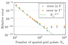
The convergence with the spatial grid size for IDO-CF is estimated by solving a linear ordinary differential equation
with the boundary conditions
| (27) |
and the analytical solution . The relative errors in the value and the derivative are estimated as
| (28) |
In Fig. 1 the relative errors are depicted as functions of the total number of spatial grid points for the proposed spatial discretisation scheme IDO-CF (Sec. 2.2). It demonstrates the convergence above the 4th order (the error is approximately proportional to ) with the spatial grid size both in the value and in the derivative of the solution. The relative errors saturate at approximately level due to finite precision arithmetics (see Sec. 4 in [37]).
3.2 Time advance convergence
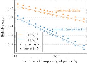
To estimate the order of convergence with the time step size, a conservation equation for particles in cylindrical geometry [34]
| (29) |
is solved using IDO-CF spatial discretisation scheme both with iRK and with BE time advance schemes. The analytical solution is
| (30) |
and the boundary conditions are given by
| (31) |
The temporal and spatial simulation domains are respectively and , and the initial condition is . The relative errors for the profile value and the derivative are estimated by Eq. (28) at and are shown in Fig. 2. As expected, the proposed IDO-CF scheme with iRK time advance demonstrates the second order convergence with the number of time steps , while the IDO-CF with BE time advance (8) has the first order convergence. In both cases, the spatial grid with was used. The error contribution due to spatial convergence is several orders of magnitude lower than the one from temporal convergence, and thus the time advance error dominates the total error.
3.3 Nonlinear convergence
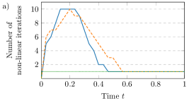
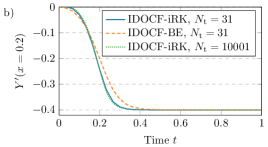
To estimate the efficiency of the nonlinear convergence scheme using Picard-type operation with under-relaxation in combination with IDO-CF space discretisation, and iRK and BE time advance, the following nonlinear partial differential equation is solved
| (32) |
where the stiff transport model for diffusivity is used
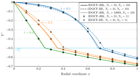
Here, and . At , the initial condition is set to . The time interval is simulated with time steps. The nonlinear convergence threshold is set and Picard operation with under-relaxation with is used in all the simulations. Fig. 3a shows the number of nonlinear iterations (calls to the transport model) at each time step for three simulations using the IDO-CF numerical scheme with the iRK (5)-(7) and BE (8) time advance. The iRK with (solid line) and BE with (dashed line) require no more than 10 iterations at each time step to converge – total amount of iterations are 105 and 117 respectively. As a reference simulation with high resolution in time domain, IDO-CF with iRK (dotted line) is used, which requires only one nonlinear iteration at each time step, that is, the total of 10001 iterations for the entire simulation. All three simulations are performed with . The corresponding time traces of at the position are given in Fig. 3b. The iRK scheme with predicts the time evolution close to the reference simulation, while the BE scheme with has noticeable discrepancies. In Fig. 4 the profiles are shown at for the three simulations described above. The critical gradient is shown by the horizontal line in cyan colour. Additionally, an iRK simulation with (circle markers) shows a good agreement with the reference simulation, thus demonstrating the robustness of the numerical scheme even for the coarse spatial grids.
The results in Figs. 3-4 demonstrate that the proposed scheme, IDO-CF with iRK time advance and under-relaxation nonlinear convergence, allows for large time steps and for reduced spatial grids, while retaining high accuracy even for stiff non-linear problems. This in turn allows to significantly reduce the numerical costs associated with calls to the physical models.
3.4 Conservation
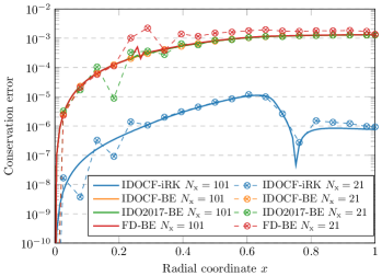
The nonlinear problem (32) was used to evaluate the conservation properties of the discretisation schemes. The normalised conservation error is estimated by integrating (32) in temporal and spatial coordinates
| (33) | |||
| (34) | |||
| (35) | |||
| (36) |
that is, the conservation error is the error in the total conserved quantity inside the flux surface , normalised to the total integrated source. The profiles and diffusivities at the converged iterations are used in evaluating the conservation errors. The integration in Eqs. (33) and (34) is performed using a cubic splines representation of integrands as a method not specific to the considered solvers for fair comparison. The time interval for evaluating the conservation is . Fig. 5 compares 4 solvers: the proposed scheme IDO-CF with iRK (blue lines), IDO-CF with BE (orange lines), our implementation of the scheme of Ref. [29] which uses BE (green lines, IDO2017), and the 2nd order finite difference solver (FD) with BE (red lines). The solid lines are for and the dashed lines with circle-cross markers are for . For all simulations . The dominant contribution to the conservation error is due to the time integration scheme, and iRK provides approximately 2 orders of magnitude lower conservation error as compared to the BE schemes. Additionally, the proposed IDO-CF scheme gives exact conservation in each spatial cell, which is ensured by including the spatially integrated equation in the system (22). FD and the scheme of [29] do not solve the spatially integrated equation exactly, and instead rely on the accuracy of the spatial discretisation scheme for conservation. For FD scheme this is demonstrated by the higher conservation error for , which due to the error from the spatial accuracy exceeds the error due to the time accuracy.
4 Conclusions
This paper presents a numerical scheme for solving transport equations for tokamak plasmas. The proposed numerical scheme has the exact conservation in spatial variable, above the 4th order of convergence in space, the 2nd order of convergence in time for the physics variable and its gradient, and a rapid non-linear convergence. This enables robust simulations on reduced spatial and temporal grids, thus minimising the amount of calls to computationally expensive physical models. The proposed scheme is compatible with non-equidistant grids.
The proposed scheme builds upon the existing numerical schemes of IDO family and provides the following advantages:
-
1.
compared to [31], the implicit time advance is used, making the scheme suitable for stiff nonlinear equations;
-
2.
compared to [38], the conservative formulation in spatial discretisation is used, ensuring conservation of cell values;
-
3.
compared to [29], which is specifically designed for plasma transport equations, our scheme has higher order of convergence in time and exact conservation in spatial coordinate. Additionally, the scheme proposed here does not require the second-order derivative of diffusivity and the first-order derivative of the source term, thus avoiding potential issues related to instabilities when taking numerical derivatives of transport coefficients computed by physical codes.
The considered numerical example with stiff transport model demonstrates that the second order time stepping method significantly improves the accuracy of the transient process modelling and the conservation properties in the simulation as compared to the first-order methods.
The proposed numerical scheme formulates the inputs in a generalised form suitable for integrated modelling codes. Modification of the scheme to account for extra terms and coefficients in the generalised form of a transport equation is straightforward, as explained in the end of Sec. 2.3. The extension of the spatial discretisation scheme IDO-CF to several spatial dimensions is described in Reference [31]. In the numerical examples we considered the diffusivity term as a source of a non-linearity, however, the non-linearities of other origin (such as coupling between transport equations) can be also taken into account inside the matrix given in Sec. 2.4.
Appendix A Coefficients for the piece-wise polynomial approximation
With and the matching conditions (12)-(15) are rewritten as
| (37) | ||||
| (38) | ||||
| (39) | ||||
| (40) |
for each th polynomial , . This system of equations is linear with respect to and the solution is
| (41) |
| (42) |
| (43) |
| (44) |
Note that are linear combinations of and and hence allow the representation . The row vectors only depend on the grid parameters and are non-zero only at the positions corresponding to the positions of in . The IDO-CF spatial discretisation scheme uses the following quantities:
| (45) |
for and in Eqs. (16) and (18), and
| (46) |
| (47) |
for in Eq.(20).
Appendix B Linear transformations
Acknowledgements
This work has received funding from the Swedish Research Council (2021-00182,“INFRAfusion”).
References
- [1] H.-T. Kim, F. Auriemma, J. Ferreira, S. Gabriellini, A. Ho, P. Huynh, K. Kirov, R. Lorenzini, M. Marin, M. Poradzinski, et al., Validation of D–T fusion power prediction capability against 2021 JET D–T experiments, Nuclear Fusion 63 (11) (2023) 112004. doi:10.1088/1741-4326/ace26d.
- [2] T. Luda, C. Angioni, M. Dunne, E. Fable, A. Kallenbach, N. Bonanomi, P. Schneider, M. Siccinio, G. Tardini, T. A. U. Team, T. E. M. Team, Integrated modeling of ASDEX Upgrade plasmas combining core, pedestal and scrape-off layer physics, Nuclear Fusion 60 (3) (2020) 036023. doi:10.1088/1741-4326/ab6c77.
- [3] D. Fajardo, C. Angioni, R. Dux, E. Fable, U. Plank, O. Samoylov, G. Tardini, the ASDEX Upgrade Team, Full-radius integrated modelling of ASDEX Upgrade L-modes including impurity transport and radiation, Nuclear Fusion 64 (4) (2024) 046021. doi:10.1088/1741-4326/ad29bd.
- [4] V. Ostuni, J. Artaud, G. Giruzzi, E. Joffrin, H. Heumann, H. Urano, Tokamak discharge simulation coupling free-boundary equilibrium and plasma model with application to JT-60SA, Nuclear Fusion 61 (2) (2021) 026021. doi:10.1088/1741-4326/abcdb7.
- [5] J. Mailloux, N. Abid, K. Abraham, P. Abreu, O. Adabonyan, P. Adrich, V. Afanasev, M. Afzal, T. Ahlgren, L. Aho-Mantila, et al., Overview of JET results for optimising ITER operation, Nuclear Fusion 62 (4) (2022) 042026. doi:10.1088/1741-4326/ac47b4.
- [6] J. Garcia, R. Dumont, J. Joly, J. Morales, L. Garzotti, T. Bache, Y. Baranov, F. Casson, C. Challis, K. Kirov, et al., First principles and integrated modelling achievements towards trustful fusion power predictions for JET and ITER, Nuclear Fusion 59 (8) (2019) 086047. doi:10.1088/1741-4326/ab25b1.
- [7] X. Litaudon, F. Jenko, D. Borba, D. V. Borodin, B. J. Braams, S. Brezinsek, I. Calvo, R. Coelho, A. J. H. Donné, O. Embréus, D. Farina, T. Görler, J. P. Graves, R. Hatzky, J. Hillesheim, F. Imbeaux, D. Kalupin, R. Kamendje, H.-T. Kim, H. Meyer, F. Militello, K. Nordlund, C. Roach, F. Robin, M. Romanelli, F. Schluck, E. Serre, E. Sonnendrücker, P. Strand, P. Tamain, D. Tskhakaya, J. L. Velasco, L. Villard, S. Wiesen, H. Wilson, F. Zonca, EUROfusion-theory and advanced simulation coordination (E-TASC): programme and the role of high performance computing, Plasma Physics and Controlled Fusion 64 (3) (2022) 034005. doi:10.1088/1361-6587/ac44e4.
- [8] D. P. Coster, V. Basiuk, G. Pereverzev, D. Kalupin, R. Zagórksi, R. Stankiewicz, P. Huynh, F. Imbeaux, et al., The european transport solver, IEEE Transactions on Plasma Science 38 (9) (2010) 2085–2092. doi:10.1109/TPS.2010.2056707.
- [9] G. Cenacchi, A. Taroni, Jetto a free boundary plasma transport code, Tech. rep., ENEA, https://inis.iaea.org/collection/NCLCollectionStore/_Public/19/097/19097143.pdf (1988).
- [10] G. V. Pereverzev, P. Yushmanov, ASTRA. Automated system for transport analysis in a tokamak, IPP 5/98https://pure.mpg.de/rest/items/item_2138238/component/file_2138237/content (2002).
- [11] M. Romanelli, G. Corrigan, V. Parail, S. Wiesen, R. Ambrosino, P. D. S. A. Belo, L. Garzotti, D. Harting, F. Köchl, T. Koskela, et al., JINTRAC: a system of codes for integrated simulation of tokamak scenarios, Plasma and Fusion research 9 (2014) 3403023–3403023. doi:10.1585/pfr.9.3403023.
- [12] N. Hayashi, T. Takizuka, T. Ozeki, N. Aiba, N. Oyama, Integrated simulation of ELM energy loss determined by pedestal MHD and SOL transport, Nuclear fusion 47 (7) (2007) 682. doi:10.1088/0029-5515/47/7/019.
- [13] M. Honda, A. Fukuyama, Dynamic transport simulation code including plasma rotation and radial electric field, Journal of Computational Physics 227 (5) (2008) 2808–2844. doi:10.1016/j.jcp.2007.11.017.
- [14] R. Hawryluk, An empirical approach to tokamak transport, in: B. Coppi, G. Leotta, D. Pfirsch, R. Pozzoli, E. Sindoni (Eds.), Physics of Plasmas Close to Thermonuclear Conditions, Pergamon, 1981, pp. 19–46. doi:10.1016/B978-1-4832-8385-2.50009-1.
- [15] J. Artaud, V. Basiuk, F. Imbeaux, M. Schneider, J. Garcia, G. Giruzzi, P. Huynh, T. Aniel, F. Albajar, J. Ané, A. Bécoulet, C. Bourdelle, A. Casati, L. Colas, J. Decker, R. Dumont, L. Eriksson, X. Garbet, R. Guirlet, P. Hertout, G. Hoang, W. Houlberg, G. Huysmans, E. Joffrin, S. Kim, F. Köchl, J. Lister, X. Litaudon, P. Maget, R. Masset, B. Pégourié, Y. Peysson, P. Thomas, E. Tsitrone, F. Turco, The cronos suite of codes for integrated tokamak modelling, Nuclear Fusion 50 (4) (2010) 043001. doi:10.1088/0029-5515/50/4/043001.
- [16] H. Grad, J. Hogan, Classical diffusion in a tokomak, Physical review letters 24 (24) (1970) 1337. doi:10.1103/PhysRevLett.24.1337.
- [17] J. Blum, J. Le Foll, Plasma equilibrium evolution at the resistive diffusion timescale, Computer Physics Reports 1 (7-8) (1984) 465–494. doi:10.1016/0167-7977(84)90013-3.
- [18] F. Jenko, W. Dorland, Nonlinear electromagnetic gyrokinetic simulations of tokamak plasmas, Plasma physics and controlled fusion 43 (12A) (2001) A141. doi:10.1088/0741-3335/43/12A/310.
- [19] J. Candy, E. Belli, R. Bravenec, A high-accuracy Eulerian gyrokinetic solver for collisional plasmas, Journal of Computational Physics 324 (2016) 73–93. doi:10.1016/j.jcp.2016.07.039.
- [20] G. Staebler, J. Kinsey, R. Waltz, Gyro-Landau fluid equations for trapped and passing particles, Physics of Plasmas 12 (10) (2005). doi:10.1063/1.2044587.
- [21] J. Citrin, C. Bourdelle, F. J. Casson, C. Angioni, N. Bonanomi, Y. Camenen, X. Garbet, L. Garzotti, T. Görler, O. Gürcan, et al., Tractable flux-driven temperature, density, and rotation profile evolution with the quasilinear gyrokinetic transport model QuaLiKiz, Plasma Physics and Controlled Fusion 59 (12) (2017) 124005. doi:10.1088/1361-6587/aa8aeb.
- [22] P. Strand, G. Bateman, A. Eriksson, W. Houlberg, A. Kritz, H. Nordman, J. Weiland, Comparisons of anomalous and neoclassical contributions to core particle transport in tokamak discharges, in: 31th EPS Conference, London, 2004.
- [23] D. Tegnered, M. Oberparleiter, H. Nordman, P. Strand, Fluid and gyrokinetic modelling of particle transport in plasmas with hollow density profiles, Journal of Physics: Conference Series 775 (1) (2016) 012014. doi:10.1088/1742-6596/775/1/012014.
- [24] E. Fransson, H. Nordman, P. Strand, JET Contributors, Upgrade and benchmark of quasi-linear transport model EDWM, Physics of Plasmas 29 (11) (2022). doi:10.1063/5.0119515.
- [25] M. Erba, A. Cherubini, V. Parail, E. Springmann, A. Taroni, Development of a non-local model for tokamak heat transport in L-mode, H-mode and transient regimes, Plasma Physics and Controlled Fusion 39 (2) (1997) 261. doi:10.1088/0741-3335/39/2/004.
- [26] A. Fukuyama, S. Takatsuka, S.-I. Itoh, M. Yagi, K. Itoh, Transition to an enhanced internal transport barrier, Plasma Physics and Controlled Fusion 40 (5) (1998) 653. doi:10.1088/0741-3335/40/5/016.
- [27] J. Breslau, M. Gorelenkova, F. Poli, J. Sachdev, A. Pankin, G. Perumpilly, X. Yuan, L. Glant, TRANSP, Computer Software https://doi.org/10.11578/dc.20180627.4 (jun 2018). doi:10.11578/dc.20180627.4.
- [28] F. Felici, J. Citrin, A. Teplukhina, J. Redondo, C. Bourdelle, F. Imbeaux, O. Sauter, JET Contributors, the EUROfusion MST1 Team, Real-time-capable prediction of temperature and density profiles in a tokamak using RAPTOR and a first-principle-based transport model, Nuclear Fusion 58 (9) (2018) 096006. doi:10.1088/1741-4326/aac8f0.
- [29] J. M. Park, M. Murakami, H. S. John, L. L. Lao, M. Chu, R. Prater, An efficient transport solver for tokamak plasmas, Computer Physics Communications 214 (2017) 1–5. doi:10.1016/j.cpc.2016.12.018.
- [30] G. Pereverzev, G. Corrigan, Stable numeric scheme for diffusion equation with a stiff transport, Computer Physics Communications 179 (8) (2008) 579–585. doi:10.1016/j.cpc.2008.05.006.
- [31] Y. Imai, T. Aoki, K. Takizawa, Conservative form of interpolated differential operator scheme for compressible and incompressible fluid dynamics, Journal of Computational Physics 227 (4) (2008) 2263–2285. doi:10.1016/j.jcp.2007.11.031.
- [32] G. Wanner, E. Hairer, Solving ordinary differential equations II, Springer Berlin Heidelberg, 1996. doi:10.1007/978-3-642-05221-7.
- [33] S. Linge, H. P. Langtangen, Nonlinear Problems, in: Finite Difference Computing with PDEs: A Modern Software Approach, Springer, Cham, 2017, pp. 353–407. doi:10.1007/978-3-319-55456-3_5.
- [34] F. Hinton, R. D. Hazeltine, Theory of plasma transport in toroidal confinement systems, Reviews of Modern Physics 48 (2) (1976) 239. doi:10.1103/RevModPhys.48.239.
- [35] B. L. Ehle, On Padé approximations to the exponential function and A-stable methods for the numerical solution of initial value problems, Ph.D. thesis, University of Waterloo, Waterloo, Ontario (1969).
- [36] L. O. Jay, Lobatto methods, in: B. Engquist (Ed.), Encyclopedia of Applied and Computational Mathematics, Springer, Berlin, Heidelberg, 2015, pp. 817–826. doi:10.1007/978-3-540-70529-1_123.
- [37] I. H. Bell, U. K. Deiters, A. M. M. Leal, Implementing an Equation of State without Derivatives: teqp, Industrial & Engineering Chemistry Research 61 (17) (2022) 6010–6027. doi:10.1021/acs.iecr.2c00237.
- [38] Y. Imai, T. Aoki, A higher-order implicit IDO scheme and its CFD application to local mesh refinement method, Computational Mechanics 38 (2006) 211–221. doi:10.1007/s00466-005-0742-x.