Note on a Theoretical Justification for Approximations of Arithmetic Forwards

Álvaro Romaniega
Internal Validation Quants - Risk Division
Santander Group
Internal Validation Quants - Risk Division - Santander Group alvaroromaniega@gmail.com, alvaro.romaniega@gruposantander.com
Abstract.

This brief note explores the theoretical justification for some approximations of arithmetic forwards ($F_{a}$) with weighted averages of overnight (ON) forwards ($F_{k}$). The central equation presented in this analysis is:

$$F_{a}(0;T_{s},T_{e})=\frac{1}{\tau(T_{s},T_{e})}\sum_{k=1}^{K}\tau_{k}\mathcal{A}_{k}F_{k}\,,$$

with $\mathcal{A}_{k}$ being explicit model-dependent quantities that, under certain market scenarios, are close to one. We will present computationally cheaper methods that approximate $F_{a}$, i.e., we will define some $\{\tilde{\mathcal{A}}_{k}\}_{k=1}^{K}$ such that

$$F_{a}(0;T_{s},T_{e})\approx\frac{1}{\tau(T_{s},T_{e})}\sum_{k=1}^{K}\tilde{\mathcal{A}}_{k}\tau_{k}F_{k}\,.$$

We also demonstrate that one of these forms can be closely aligned with an approximation suggested by Katsumi Takada in his work on the valuation of arithmetic averages of Fed Funds rates.

I would like to thank CΓ©sar Romaniega for his thorough revision of the manuscript. I would also like to thank the IR internal validation team of Risk Division - Santander Group for the useful discussions that led to the writing of this manuscript.

Disclaimer

The views and opinions expressed in this note are those of the author and do not necessarily reflect the official policy or position of Santander Group.

1. Introduction

In the realm of financial markets, various interest rate products are actively traded, such as interest rate swaps, basis swaps, and cross-currency swaps. Among these, the valuation of forward rates and their respective structures play a crucial role in pricing and risk management. One notable aspect of this valuation process involves the arithmetic average of overnight (ON) forward rates and its approximation.

Arithmetic averages of ON rates are particularly relevant in contexts where the Fed Funds (FF) rate is used, as seen in FF-LIBOR basis swaps. While ON rates are often compounded daily in financial instruments like overnight index swaps, the arithmetic average of these rates offers a different perspective that requires careful consideration and adjustment for accurate valuation. This note aims to demonstrate the conditions under which arithmetic forwards can be closely approximated by a weighted average of the ON forwards. In particular, this aligns with an approximation given by some platforms, such as Murex, which provides the expression:

$$F_{a}^{\text{Murex}}(0;T_{s},T_{e})\coloneqq\frac{1}{\tau(T_{s},T_{e})}\sum_{k=1}^{K}\tau_{k}F_{k}\,.$$

We will provide a theoretical and numerical discussion on under which market scenarios this approximation can be considered accurate and consider alternative and more accurate approximations. We also demonstrate that one of these forms can be closely aligned with an approximation suggested by Katsumi Takada in his work on the valuation of arithmetic averages of Fed Funds rates. See also [Sko24] for a new approach in computing the convexity adjustment particularized for the SABR model.

2. Notation

In this note, we use the following notation:

  • β€’

    Ts,Tesubscript𝑇𝑠subscript𝑇𝑒T_{s},T_{e}: The start and end dates of the interest period.

  • β€’

    rπ‘Ÿr: The (collateralized) interest rate.

  • β€’

    P​(t,T)𝑃𝑑𝑇P(t,T): The price at time $t$ of a zero-coupon bond maturing at time $T$. $P(T):=P(0,T)$, i.e., the price at time 0 of a zero-coupon bond maturing at time $T$.

  • β€’

    Ο„ksubscriptπœπ‘˜\tau_{k}: The day count fraction, according to a given day-count convention, for the $k$-th day, $T_{k}$, within the interest period $\left[T_{s},T_{e}\right]$. That is, it is the disjoint union,

    $$[T_{s},T_{e})=\bigsqcup_{k=1}^{K}[T_{k},T_{k+1})$$
  • β€’

    τ​(Ts,Te)𝜏subscript𝑇𝑠subscript𝑇𝑒\tau(T_{s},T_{e}): The day count fraction for the entire interest period $\left[T_{s},T_{e}\right]$.

  • β€’

    𝔼⋅superscript𝔼⋅\mathbb{E}^{\cdot}: The expectation operator, where the superscript denotes the measure under which the expectation is taken. Different measures used in this document include:

    • –

      𝔼Qsuperscript𝔼𝑄\mathbb{E}^{Q}: The risk-neutral measure. Under this measure, the discounted price of a traded asset is a martingale. The numeraire is the money market account, that we denote by $B$.

    • –

      𝔼Tk≔𝔼QTk≔superscript𝔼subscriptπ‘‡π‘˜superscript𝔼superscript𝑄subscriptπ‘‡π‘˜\mathbb{E}^{T_{k}}\coloneqq\mathbb{E}^{Q^{T_{k}}}: The $T_{k}$-forward measure. Under this measure, the price of a zero-coupon bond maturing at time $T_{k}$ is used as the numeraire.

    • –

      𝔼Te≔𝔼QTe≔superscript𝔼subscript𝑇𝑒superscript𝔼superscript𝑄subscript𝑇𝑒\mathbb{E}^{T_{e}}\coloneqq\mathbb{E}^{Q^{T_{e}}}: The $T_{e}$-forward measure. Under this measure, the price of a zero-coupon bond maturing at time $T_{e}$ is used as the numeraire.

  • β€’

    {Rk}k=1,2,…,Ksubscriptsubscriptπ‘…π‘˜π‘˜12…𝐾\{R_{k}\}_{k=1,2,\ldots,K}: The effective overnight rates fixed in the interest period $\left[T_{s},T_{e}\right]$.

  • β€’

    Rg​(Ts,Te)subscript𝑅𝑔subscript𝑇𝑠subscript𝑇𝑒R_{g}(T_{s},T_{e}): The daily compounded ON rate over the interest period $\left[T_{s},T_{e}\right]$, defined as:

    $$R_{g}(T_{s},T_{e}):=\frac{1}{\tau(T_{s},T_{e})}\left(\prod_{k=1}^{K}(1+\tau_{k}R_{k})-1\right)\,.$$
  • β€’

    Ra​(Ts,Te)subscriptπ‘…π‘Žsubscript𝑇𝑠subscript𝑇𝑒R_{a}(T_{s},T_{e}): The arithmetic average of ON rates (AAON) over the interest period $\left[T_{s},T_{e}\right]$, defined as:

    $$R_{a}(T_{s},T_{e}):=\frac{\sum_{k=1}^{K}\tau_{k}R_{k}}{\tau(T_{s},T_{e})}\,.$$
  • β€’

    Forward Contract: A forward contract based on a given rate $R$ is an agreement to exchange a specified amount of cash flow at a future date based on the interest rate $R$ determined over a certain period. If $V_{t}$ is the value of the floating leg at time $t$, we can define the forward at time $t$:

    $$F(t;T_{s},T_{e}):=\frac{V_{t}}{\tau(T_{s},T_{e})P(T_{e})}\,.$$
  • β€’

    The (simply-compounded) forward rate, at time $t=0$, associated with the $k$-th period within the interest interval $\left[T_{s},T_{e}\right]$, which can be defined as:

    $$F_{k}\coloneqq\frac{1}{\tau_{k}}\left(\frac{P(T_{k})}{P(T_{k+1})}-1\right)\,.$$

3. Unweighted approximation

3.1. Main derivation

The present value of the floating leg at time $t=0$ with an AAON over the interest period $\left[T_{s},T_{e}\right]$ with unit nominal amount is given by

$\displaystyle V_{0}^{a}$ $\displaystyle=\mathbb{E}^{Q}\left(e^{-\int_{0}^{T_{e}}r(u)du}\tau\left(T_{s},T_{e}\right)R_{a}\right)$
$\displaystyle=\mathbb{E}^{Q}\left(e^{-\int_{0}^{T_{e}}r(u)du}\sum_{k=1}^{K}\tau_{k}R_{k}\right)\,.$

By linearity,

$$V_{0}^{a}=\sum_{k=1}^{K}\tau_{k}\mathbb{E}^{Q}\left(e^{-\int_{0}^{T_{e}}r(u)du}R_{k}\right)\,.$$

Given that $r\geq 0$ and $T_{k}\leq T_{e}$, there exist $\{A_{k}\}_{k=1}^{K}$ with $A_{k}\leq 1$ such that

$$\sum_{k=1}^{K}\tau_{k}\mathbb{E}^{Q}\left(e^{-\int_{0}^{T_{e}}r(u)du}R_{k}\right)=\sum_{k=1}^{K}\tau_{k}A_{k}\mathbb{E}^{Q}\left(e^{-\int_{0}^{T_{k}}r(u)du}R_{k}\right)\,,$$

with, heuristically speaking,

$$A_{k}\approx\frac{\mathbb{E}^{Q}\left(e^{-\int_{0}^{T_{e}}r(u)du}\right)}{\mathbb{E}^{Q}\left(e^{-\int_{0}^{T_{k}}r(u)du}\right)}=\frac{P(T_{e})}{P(T_{k})}\,,$$

see Section 3.2 for further justification. We can define the numeraire $N_{t}^{k}:=P(t,T_{k})$ and perform multiple changes of measure such that

$$\sum_{k=1}^{K}\tau_{k}A_{k}\mathbb{E}^{Q}\left(e^{-\int_{0}^{T_{k}}r(u)du}R_{k}\right)=\sum_{k=1}^{K}\tau_{k}A_{k}P(T_{k})\mathbb{E}^{T_{k}}\left(R_{k}\right)\,.$$

By (146) of [AB13] (see also above (6.47) in [AP10a], cf. Lemma 4.2.3 there),

$$\mathbb{E}^{T_{k}}\left(R_{k}\right)=F_{k}\,,$$

the forward associated with the date $T_{k}$. All in all,

$$V_{0}^{a}=\sum_{k=1}^{K}\tau_{k}A_{k}P(T_{k})F_{k}=P(T_{e})\sum_{k=1}^{K}\tau_{k}\mathcal{A}_{k}F_{k}\,,$$ (1)

where we have define our arithmetic factors as

$$\mathcal{A}_{k}:=A_{k}\frac{P(T_{k})}{P(T_{e})}\,.$$

These are model-dependent quantities that under the aforementioned approximation are close to one. Indeed, as mentioned above,

$$\mathcal{A}_{k}\approx\frac{P(T_{e})}{P(T_{k})}\frac{P(T_{k})}{P(T_{e})}=1\,.$$ (2)

Thus, see also Equation (12) in [Tak11] for a slightly different definition, by definition and (1),

$$F_{a}(0;T_{s},T_{e}):=\frac{V_{0}^{a}}{\tau(T_{s},T_{e})P(T_{e})}=\frac{1}{\tau(T_{s},T_{e})}\sum_{k=1}^{K}\tau_{k}\mathcal{A}_{k}F_{k}\,.$$

Using the approximation of (2) then

$$F_{a}(0;T_{s},T_{e})\approx\frac{1}{\tau(T_{s},T_{e})}\sum_{k=1}^{K}\tau_{k}F_{k}\,.$$

3.2. Heuristics justification and closed form of the arithmetic factor $\mathcal{A}_{k}$

By definition, with $B(t):=e^{\int_{0}^{t}r}$ the money market account with the collateralized rate,

$$A_{k}=\frac{\mathbb{E}^{Q}\left(R_{k}B^{-1}(T_{e})\right)}{\mathbb{E}^{Q}\left(R_{k}B^{-1}(T_{k})\right)}=\frac{\mathbb{E}^{T_{e}}\left(R_{k}\right)P(T_{e})}{\mathbb{E}^{T_{k}}\left(R_{k}\right)P(T_{k})}\rightarrow\mathcal{A}_{k}=\frac{\mathbb{E}^{T_{e}}\left(R_{k}\right)}{\mathbb{E}^{T_{k}}\left(R_{k}\right)}\,,$$

where we have used the change of numeraire formula twice. We know111We are considering the simpler case, $t=0$, where $\mathcal{F}_{0}$ is the trivial $\sigma$-algebra. For the case $t>0$, we would use Abstract Bayes’ Theorem, for instance, Appendix C.3 of [Bjo20] or page 9 of [AP10a], for measures $P,Q$, with Radon-Nikodym derivative $L$ and a $\mathcal{F}_{T}$-measurable function $X$, $$\mathbb{E}^{Q}\left({X}|\mathcal{F}_{t}\right)=\mathbb{E}^{P}\left(X\frac{L_{T}}{L_{t}}\bigg{|}\mathcal{F}_{t}\right)\,.$$ , for instance, Chapter 15 of [Bjo20] or Theorem 1.4.2 of [AP10a], that the likelihood process, for a given filtration $\{\mathcal{F}_{t}\}_{t}$, is

$$L_{t}^{k}:=\frac{dQ^{T_{k}}}{dQ^{T_{e}}}\bigg{|}_{\mathcal{F}_{t}}=\frac{P(t,T_{k})/P(T_{k})}{P(t,T_{e})/P(T_{e})}\,,$$

so we arrive at the expression

$$\mathbb{E}^{{T_{k}}}\left(R_{k}\right)=\mathbb{E}^{{T_{e}}}\left(R_{k}\cdot\frac{P(T_{e})}{P(T_{k},T_{e})P(T_{k})}\right)\,.$$

Therefore,

$$\mathcal{A}_{k}=\mathbb{E}^{{T_{e}}}\left(\frac{R_{k}}{\mathbb{E}^{{T_{e}}}(R_{k})}\cdot\frac{P(T_{e})}{P(T_{k},T_{e})\cdot P(T_{k})}\right)^{-1}\,,$$

where the economic interpretation of the second term corresponds to the strategy of rolling the bond versus not rolling it at $T_{k}$. Using the martingale pricing formula for a given numeraire,

$$\mathbb{E}^{T_{e}}\left(\frac{1}{P(T_{k},T_{e})}\right)=\mathbb{E}^{Q}\left(\frac{1}{B(T_{k})}\right)\frac{1}{P(0,T_{e})}=\frac{P(T_{k})}{P(T_{e})}\,.$$ (3)

Thus, finally,

$$\mathcal{A}_{k}=\mathbb{E}^{T_{e}}\left(\frac{R_{k}}{\mathbb{E}^{T_{e}}(R_{k})}\cdot\frac{P(T_{k},T_{e})^{-1}}{\mathbb{E}^{T_{e}}(P(T_{k},T_{e})^{-1})}\right)^{-1}\,.$$ (4)

Intuitively, this expression is close to one as it represents the expectation of two random variables that each have an expectation of one. Trivial sufficient conditions for the approximation to hold are:

  1. (1)

    If $T_{k}$ is close to $T_{e}$, then $P(T_{k},T_{e})\approx 1$. Therefore,

    $$\mathcal{A}_{k}\approx\mathbb{E}^{{T_{e}}}\left(\frac{R_{k}}{\mathbb{E}^{{T_{e}}}(R_{k})}\cdot 1\right)^{-1}=1\,.$$
  2. (2)

    If interest rate volatility is low for the $[T_{k},T_{k+1}]$-forward, so, $R_{k}\approx\mathbb{E}^{T_{e}}(R_{k})$. Thus,

    $$\mathcal{A}_{k}\approx\mathbb{E}^{{T_{e}}}\left(1\cdot\frac{P(T_{k},T_{e})^{-1}}{\mathbb{E}^{T_{e}}(P(T_{k},T_{e})^{-1})}\right)^{-1}=1\,.$$
  3. (3)

    Obviously, for deterministic rates the quantity is exactly one.

4. Refined approximation formula

Although the arithmetic factors are generally close to one, this approximation can be far from accurate if, for instance, interest rate volatility is high and we are far from the end date. For the sake of conciseness, assume that the evolution of the instantaneous short-rate process under the risk-neutral measure $Q$ is given by a Markovian222Understood in the sense of Proposition 12.1.1 of [AP10b]. There, as the instantaneous forward rate is $f(t,T)=f(0,T)+\Omega(t,T)+h(T)^{\top}z(t)$, i.e., a function of the state variables $z$ at $t$ and some deterministic functions, then $$P(t,T)=e^{-\int_{t}^{T}f(t,u)du}=e^{\int_{t}^{T}(f(0,u)+\Omega(t,u))du+\left(\int_{t}^{T}h(u)^{\top}du\right)\cdot z(t)}=P(t,T,z(t))\,.$$ $n$-factor model:

$$r(t)=\sum_{i=1}^{n}x_{i}(t)+\varphi(t)=\sum_{i=0}^{n}x_{i}(t),\quad r(0)=r_{0},$$ (5)

where $x_{0}(t)\coloneqq\varphi(t)$ and the ItΓ΄ processes $\{x_{i}(t):t\geq 0\}_{i=1}^{n}$ satisfy the following stochastic differential equations (Ornstein–Uhlenbeck process):

$$\begin{cases*}dx_{i}(t)=-a_{i}x_{i}(t)dt+\sigma_{i}dW_{i}(t),\\ x_{i}(0)=0,\end{cases*}\quad i=1,\ldots,n\,.$$

Here, $\left(W_{i}(t)\right)_{i=1}^{n}$ is a $n$-dimensional Brownian motion with instantaneous correlations given by the quadratic covariation:

$$\langle W_{i}(t),W_{j}(t)\rangle=\rho_{ij}t,\quad\text{for}\;i,j=1,\ldots,n,$$ (6)

where $r_{0},a_{i},\sigma_{i}$ are positive constants, $\rho_{ij}$ are the correlation coefficients with $-1\leq\rho_{ij}\leq 1$, and $\varphi(t)$ is a deterministic function that recovers the spot discount curve given by the market, $P^{M}(0,T)$. We denote by $\mathcal{F}_{t}$ the $\sigma$-field generated333More precisely, see Definition 9.19 of [Dri19], $$\mathcal{F}_{t}:=\sigma\left(x(s),s\leq t\right):=\sigma\left(\bigcup_{s\leq t}x(s)^{-1}(\mathcal{B}(\mathbb{R}^{n}))\right)=\text{minimal }\sigma\text{-algebra such that all }x(s)\text{ are measurable.}$$ by the processes $x(t)\coloneqq\left(x_{i}(t)\right)_{i=1}^{n}$ up to time $t$. Therefore,

$\displaystyle P(t,T)$ =𝔼Q​(exp⁑(βˆ’βˆ«tTrs​𝑑s)|β„±t)(martingale measure)absentsuperscript𝔼𝑄conditionalsuperscriptsubscript𝑑𝑇subscriptπ‘Ÿπ‘ differential-d𝑠subscriptℱ𝑑(martingale measure)\displaystyle=\mathbb{E}^{Q}\left(\exp\left(-\int_{t}^{T}r_{s}ds\right)\bigg{|}\mathcal{F}_{t}\right)\quad\text{(martingale measure)}
=𝔼Q​(exp⁑(βˆ’βˆ«tTrs​𝑑s)|σ​(xt1,xt2,…,xtn))(Markovian property)absentsuperscript𝔼𝑄conditionalsuperscriptsubscript𝑑𝑇subscriptπ‘Ÿπ‘ differential-dπ‘ πœŽsuperscriptsubscriptπ‘₯𝑑1superscriptsubscriptπ‘₯𝑑2…superscriptsubscriptπ‘₯𝑑𝑛(Markovian property)\displaystyle=\mathbb{E}^{Q}\left(\exp\left(-\int_{t}^{T}r_{s}ds\right)\bigg{|}\sigma\left(x_{t}^{1},x_{t}^{2},\ldots,x_{t}^{n}\right)\right)\quad\text{(Markovian property)}
=𝔼Q​(exp⁑(βˆ’βˆ«tT(βˆ‘i=0nxsi)​𝑑s)|σ​(xt1,xt2,…,xtn))(definition ofΒ rs)absentsuperscript𝔼𝑄conditionalsuperscriptsubscript𝑑𝑇superscriptsubscript𝑖0𝑛superscriptsubscriptπ‘₯𝑠𝑖differential-dπ‘ πœŽsuperscriptsubscriptπ‘₯𝑑1superscriptsubscriptπ‘₯𝑑2…superscriptsubscriptπ‘₯𝑑𝑛(definition ofΒ rs)\displaystyle=\mathbb{E}^{Q}\left(\exp\left(-\int_{t}^{T}\left(\sum_{i=0}^{n}x_{s}^{i}\right)ds\right)\bigg{|}\sigma\left(x_{t}^{1},x_{t}^{2},\ldots,x_{t}^{n}\right)\right)\quad\text{(definition of $r_{s}$)}
$\displaystyle=H_{t}^{T}(x_{t}^{1},x_{t}^{2},\ldots,x_{t}^{n})\,,\quad\text{(Factorization Lemma)}$

where $x_{t}=(x_{t}^{1},x_{t}^{2},\ldots,x_{t}^{n})$ and see [Dri19, Lemma 9.42] for the Factorization Lemma (Doob–Dynkin Lemma), which guarantees the existence 444This step is usually avoided unconsciously, cf. the law of the unconscious statistician, by making a notation convention for a random variable $X$, $\mathbb{E}(F|\sigma(X))=:\mathbb{E}(F|X)$, a mathematical statement, $\exists~{}H$ measurable such that $\mathbb{E}(F|\sigma(X))=H(X)$. Actually, for a particular value $x$, $\mathbb{E}(F|X=x)\coloneqq H(x)$; see, for instance, the discussion below Lemma 1.2 in [Sha03]. of the measurable function $H_{t}^{T}$. Thus, using that

$$R_{k}=\frac{1}{\tau_{k}}\left(\frac{1}{P(T_{k},T_{k+1})}-1\right)$$

and

$$P(T_{k},T_{k+1})=H_{T_{k}}^{T_{k+1}}(x_{T_{k}})\,,\,P(T_{k},T_{e})=H_{T_{k}}^{T_{e}}(x_{T_{k}})\,,$$

we can compute the arithmetic factors $\mathcal{A}_{k}$ in (4) using a numerical method as we know the distribution, or an approximation, of the random vector $x_{T_{k}}$ so it is a simple expectation. Hereafter, for the sake of simplicity and clarity, consider the G2++ model, that is, just two factors $(x_{t},y_{t})$ [BM06, Chapter 4]. We know that555For a general Multi-Factor Gaussian model see Corollary 12.1.3 of [AP10b]., [BM06, Corollary 4.2.1],

$\displaystyle V(t,T)$ $\displaystyle=\frac{\sigma^{2}}{a^{2}}\left[T-t+\frac{2}{a}e^{-a(T-t)}-\frac{1}{2a}e^{-2a(T-t)}-\frac{3}{2a}\right]$ (7)
$\displaystyle\quad+\frac{\eta^{2}}{b^{2}}\left[T-t+\frac{2}{b}e^{-b(T-t)}-\frac{1}{2b}e^{-2b(T-t)}-\frac{3}{2b}\right]$
$\displaystyle\quad+2\rho\frac{\sigma\eta}{ab}\left[T-t+\frac{e^{-a(T-t)}-1}{a}+\frac{e^{-b(T-t)}-1}{b}-\frac{e^{-(a+b)(T-t)}-1}{a+b}\right]$

and

$$P(t,T,x_{t},y_{t})=\frac{P^{M}(0,T)}{P^{M}(0,t)}\exp\left\{A(t,T,x_{t},y_{t})\right\}\,,$$ (8)

where

$$A(t,T,x_{t},y_{t}):=\frac{1}{2}\left[V(t,T)-V(0,T)+V(0,t)\right]-\left[\frac{1-e^{-a(T-t)}}{a}x(t)+\frac{1-e^{-b(T-t)}}{b}y(t)\right]\,,$$ (9)

and $P^{M}$ market bonds. As G2++ fits the spot discount bonds, $P^{M}$, then

$$\frac{P(T_{e})}{P(T_{k},T_{e})\cdot P(T_{k})}=\exp\left\{-A(T_{k},T_{e},x_{T_{k}},y_{T_{k}})\right\}\,.$$

Since $V(t,T)$ is a function depending only on the tenor, i.e., $V(t,T)=\tilde{V}(T-t)$ with $\tilde{V}(0)=0$. By Taylor’s Theorem, $\tilde{V}(T)=\tilde{V}(t)+O(T-t)$ with the constant depending only on the model parameters. Therefore, we can arrive at:

$\displaystyle\frac{P(T_{k},T_{e})\cdot P(T_{k})}{P(T_{e})}$ $\displaystyle=1+O(T_{e}-T_{k})-(x_{T_{k}}+y_{T_{k}})(T_{e}-T_{k})$
$\displaystyle-\frac{1}{2}(a\cdot x_{T_{k}}^{2}+b\cdot y_{T_{k}}^{2})(T_{e}-T_{k})^{2}+o_{x,y}\left((T_{e}-T_{k})^{2}\right)\,,$

where the little-o term depends on the stochastic factors at time $T_{k}$, not just the model parameters. Thus, heuristically, given this linear bound, (4), and the fact that if $T_{k}=T_{e}$, $\mathcal{A}_{k}=1$, we can propose the simple linear approximation:

$$\mathcal{A}_{k}^{\text{lin}}\coloneqq\mathcal{A}_{1}+(T_{k}-T_{1})\frac{1-\mathcal{A}_{1}}{T_{e}-T_{1}}\,.$$

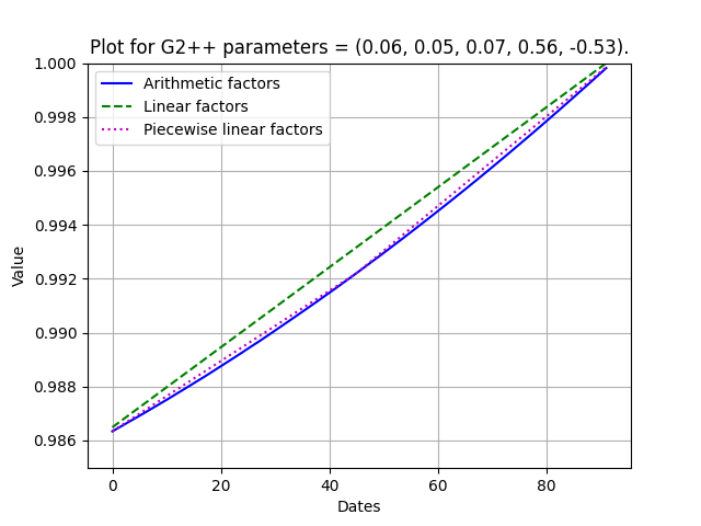
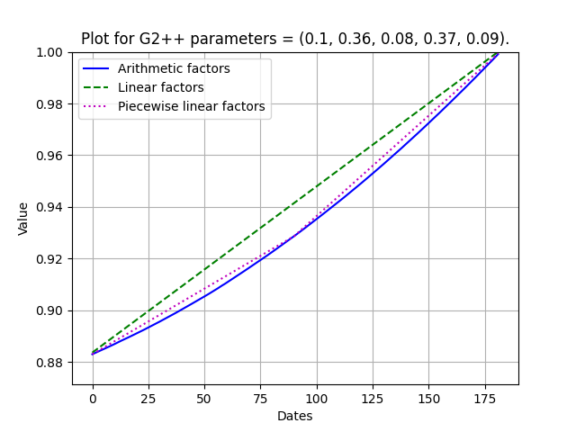
The obvious advantage of this formulation is that, while taking into account the β€œconvexity” adjustment of arithmetic forwards, we just need to compute the expectation once, not for every $k$, reducing the computational cost. From the expression above, we can see that the quadratic term of the stochastic factors and, in general, the convexity of the bond price function, will generally make this approximation an upper bound. Obviously, we can refine this approximation by taking a midpoint and performing a piecewise linear interpolation, so we can account for the curvature of the arithmetic factors with respect to the tenor, see Figure 1. That is,

$$\mathcal{A}_{k}^{\text{pw}}=\begin{cases}\mathcal{A}_{1}+(T_{k}-T_{1})\frac{\mathcal{A}_{m}-\mathcal{A}_{1}}{T_{m}-T_{1}},&\text{for }k\leq m\\ \mathcal{A}_{m}+(T_{k}-T_{m})\frac{1-\mathcal{A}_{m}}{T_{e}-T_{m}},&\text{for }k\geq m\end{cases}$$

where $T_{m}$ is the time at the midpoint.

4.1. Numerical simulations

For the sake of simplicity, take a spot discount curve with a constant discount rate of $r=0.05$ and some random parameters.

$(\sigma,a,\eta,b,\rho)$ $\mathcal{A}_{1}$ $F_{a}$ ${F_{a}^{\text{Murex}}}/{F_{a}}-1$ ${F_{a}^{\text{lin}}}/{F_{a}}-1$ ${F_{a}^{\text{pw}}}/{F_{a}}-1$
(0.07, 0.51, 0.04, 0.86, -0.27) 0.99819 0.04992 0.00176 0.00087 0.00022
(0.03, 0.46, 0.05, 0.67, -0.32) 0.99892 0.04995 0.00104 0.00050 0.00013
(0.01, 0.1, 0.08, 0.44, 0.5) 0.99710 0.04986 0.00285 0.00141 0.00036
(0.03, 0.58, 0.02, 0.41, 0.19) 0.99917 0.04996 0.00081 0.00039 0.00010
(0.02, 0.31, 0.05, 0.17, -0.61) 0.99920 0.04996 0.00079 0.00040 0.00010
Table 1. Results for $T_{s}=1$ month and $T_{e}-T_{s}=3$ months. $F_{a}$ was computed using Monte Carlo with $10^{5}$ simulations. The linear approximation reduces the error by a factor of 2, and the piecewise linear approximation reduces the error by a factor of 4 with respect to the linear one.
$(\sigma,a,\eta,b,\rho)$ $\mathcal{A}_{1}$ $F_{a}$ ${F_{a}^{\text{Murex}}}/{F_{a}}-1$ ${F_{a}^{\text{lin}}}/{F_{a}}-1$ ${F_{a}^{\text{pw}}}/{F_{a}}-1$
(0.02, 0.62, 0.09, 0.56, -0.57) 0.96287 0.04895 0.02152 0.00266 0.00062
(0.07, 0.1, 0.04, 0.5, 0.7) 0.91823 0.04763 0.04980 0.00711 0.00170
(0.04, 0.47, 0.09, 0.97, 0.17) 0.96060 0.04888 0.02288 0.00284 0.00069
(0.04, 0.98, 0.09, 0.98, 0.02) 0.96325 0.04896 0.02138 0.00271 0.00061
(0.08, 0.04, 0.08, 0.41, -0.79) 0.97871 0.04938 0.01273 0.00201 0.00048
Table 2. Results for $T_{s}=12$ months and $T_{e}-T_{s}=6$ months. $F_{a}$ was computed using Monte Carlo with $10^{5}$ simulations. The linear approximation reduces the error by a factor of 8, and the piecewise linear approximation reduces the error by a factor of 4 with respect to the linear one.
Refer to caption
(a) $T_{e}-T_{s}=$3 months.
Refer to caption
(b) $T_{e}-T_{s}=$6 months.
Figure 1. Plot of $(\mathcal{A}_{k})_{k=1}^{K}$ in blue, $(\mathcal{A}^{\text{lin}}_{k})_{k=1}^{K}$ in green, and $(\mathcal{A}^{\text{pw}}_{k})_{k=1}^{K}$ in pink. $T_{s}=12$ months. $\mathcal{A}_{k}$ was computed using Monte Carlo with $10^{6}$ simulations.
Remark 4.1.

If $T_{s}$ is close to zero, then the volatility of $r(T_{1})$ is low, see [BM06, (4.19)], so point (2) of the previous section applies, i.e.,

$$\mathcal{A}_{1}\approx\mathbb{E}^{{T_{e}}}\left(1\cdot\frac{P(T_{1},T_{e})^{-1}}{\mathbb{E}^{T_{e}}(P(T_{1},T_{e})^{-1})}\right)^{-1}=1\,.$$

$\mathcal{A}_{1}$ is also close to one, as is $\mathcal{A}_{K}$, which is close to one because of item (1) of the previous section. Thus, the plot of $\mathcal{A}_{k}$ can present a U-shaped curve. ∎

As we can see from the plots, $\mathcal{A}_{1}\leq 1$. Let us prove this. For the sake of simplicity, consider the one-factor model (that is, Hull-White or Hagan’s LGM model).

Proposition 4.2.

Let $n=1$ and $\varkappa(t)=\varkappa$ a constant, then

$$\mathcal{A}_{k}\leq 1\quad\text{for all }k\in\{1,\ldots,K\}\,.$$
Proof.

To simplify the proof, let us work in the HJM framework, following Andersen and Piterbarg’s book. It is easier if we work with the expression,

$$\mathcal{A}_{k}=\frac{\mathbb{E}^{T_{e}}\left(R_{k}\right)}{\mathbb{E}^{T_{k}}\left(R_{k}\right)}\,.$$

By [AP10b, Remark 10.1.8], the discount bond dynamics for $P(t,T)$ are given by

$$dP(t,T)/P(t,T)=r(t)dt-\sigma_{P}(t,T)dW(t),\quad\sigma_{P}(t,T)=\sigma_{r}(t)G(t,T)\,,$$

with $G(t,T)\coloneqq\int_{t}^{T}e^{-\int_{t}^{u}\varkappa(s)ds}du$, $\sigma_{r}$ the short rate volatility (now a deterministic function), and $\varkappa$ the mean reversion speed. That is, if $x(t)\coloneqq r(t)-f(0,t)$ by [AP10b, Proposition 10.1.7],

$$dx(t)=(y(t)-\varkappa(t)r(t))dt+\sigma_{r}(t)dW(t)\,.$$

Thus, as the SDE with deterministic functions as coefficients,

$$dx(t)=(Ax(t)+\tilde{B}(t))dt+C(t)dW(t)\,,$$

admits the unique solution

x​(t)=eA​t​x​(0)+∫0teA​(tβˆ’s)​(B~​(s)​d​s+C​(s)​d​W​(s)),π‘₯𝑑superscript𝑒𝐴𝑑π‘₯0superscriptsubscript0𝑑superscript𝑒𝐴𝑑𝑠~π΅π‘ π‘‘π‘ πΆπ‘ π‘‘π‘Šπ‘ x(t)=e^{At}x(0)+\int_{0}^{t}e^{A(t-s)}(\tilde{B}(s)ds+C(s)dW(s))\,,

we can solve our equation considering the case of $\varkappa(t)=\varkappa$ a constant. Using [AP10a, Equation (4.34)], Girsanov’s Theorem reads as

$$dW^{T}(t)=dW(t)+\sigma_{P}(t,T)dt\,,$$

where $W^{T}$ is a $Q^{T}$-Brownian motion. This introduces a new term in the drift, in particular in $\tilde{B}$, of the form $-\sigma_{r}^{2}(t)G(t,T)$. For $T^{\prime}\geq T$, $\sigma_{r}^{2}(t)G(t,T^{\prime})\geq\sigma_{r}^{2}(t)G(t,T)$. Thus, if $X\mid_{Q}$ denotes the distribution of the random variable $X$ under the measure $Q$, if $X^{T^{\prime}}_{t}\sim x(t)\mid_{Q^{T^{\prime}}}$, then

$$X^{T}_{t}:=X^{T^{\prime}}_{t}+\beta(t)\sim x(t)\mid_{Q^{T}}\,,$$

where

$$\beta(t)\coloneqq\int_{0}^{t}\left(e^{-\varkappa(t-s)}\left(\sigma_{r}^{2}(t)G(t,T^{\prime})-\sigma_{r}^{2}(t)G(t,T)\right)\right)\geq 0$$

is a deterministic function. As [AP10b, Proposition 10.1.7],

$$P(t,T,x(t))=\frac{P(0,T)}{P(0,t)}\exp\left(-x(t)G(t,T)-\frac{1}{2}y(t)G(t,T)^{2}\right)\,,$$

thus666Using the aforementioned law of the unconscious statistician.,

$$\mathbb{E}^{T_{k}}\left(\frac{1}{P(T_{k},T_{k+1},x(T_{k}))}\right)=\mathbb{E}^{T_{e}}\left(\frac{1}{P(T_{k},T_{k+1},x(T_{k})+\beta(T_{k}))}\right)\geq\mathbb{E}^{T_{e}}\left(\frac{1}{P(T_{k},T_{k+1},x(T_{k}))}\right)\,,$$

as $G(T_{k},T_{k+1})>0.$ ∎

5. Connection with Takada’s approximation

In this section, we explore the relationship between the approximation developed in the previous sections and an approximation suggested by Katsumi Takada in [Tak11]. Takada’s work provides valuable insights into the valuation of interest rate derivatives involving Fed Funds rates. Takada’s approximation addresses the valuation of the arithmetic average ON rates and the necessary convexity adjustments relative to daily compounded ON rates. We start with the following trivial expression:

$$\sum\tau_{k}\cdot F_{k}=\log\left(e^{\sum\tau_{k}F_{k}}\right)\,.$$ (10)

Given that $e^{x}=1+x+o(x)$ for small $x$. In this case, $o(x)>0$ for positive values of $x$. Therefore, using the definition of little-o,

$$e^{\sum_{k=1}^{K}\tau_{k}F_{k}}=\prod_{k=1}^{K}e^{\tau_{k}F_{k}}=\prod_{k=1}^{K}\left(1+\tau_{k}F_{k}+o\left(\tau_{k}F_{k}\right)\right)=\prod_{k=1}^{K}\left(1+\tau_{k}F_{k}\right)+\sum_{k=1}^{K}o\left(\mu^{k}\right)\,,$$

being $\mu\coloneqq\max_{k}{\tau_{k}F_{k}}$. Thus,

$$e^{\sum_{k=1}^{K}\tau_{k}F_{k}}=\prod_{k=1}^{K}\left(1+\tau_{k}F_{k}\right)+o\left(\mu\right)\,,$$

being the error term strictly positive. Expanding the leading term, this is equal to:

$\displaystyle\log\left(\prod_{k=1}^{K}(1+\tau_{k}F_{k})\right)$ $\displaystyle=\log\left(\prod_{k=1}^{K}\frac{P(T_{k})}{P(T_{k+1})}\right)$
$\displaystyle=\log\left(\frac{P(T_{s})}{P(T_{e})}\right)\equiv\log\left(1+\tau(T_{s},T_{e})F_{g}(0;T_{s},T_{e})\right)\,,$

where the last equality follows by the definition of continuously compounded or geometric forwards and a telescopic cancellation for the product. Therefore, we obtain, cf. (7) and (8) of [Tak11] or (145) of [AB13],

$$\sum\tau_{k}\cdot F_{k}\approx\log\left(1+\tau(T_{s},T_{e})F_{g}(0;T_{s},T_{e})\right)=\tau(T_{s},T_{e})\cdot O^{\text{det}}_{a}(0;T_{s},T_{e})\,,$$ (11)

following (13) of [Tak11], a deterministic version of Takada’s forward definition, which he denotes by $O_{a}(0;T_{s},T_{e})$. That is,

$${O}_{a}(0;T_{s},T_{e})\coloneqq\frac{1}{\tau(T_{s},T_{e})}\mathbb{E}^{T_{e}}\left(\int_{T_{s}}^{T_{e}}r\right)\,$$

and for deterministic rates $O^{\text{det}}_{a}(0;T_{s},T_{e})=O_{a}(0;T_{s},T_{e})$. Thus, if $\mathcal{A}_{k}\approx 1$, the forward rate approximation $F_{a}(0,T_{s},T_{e})$ is given by:

$$F_{a}(0,T_{s},T_{e})\approx O^{\text{det}}_{a}(0;T_{s},T_{e})>O_{a}(0,T_{s},T_{e})\,,$$ (12)

by (15) of [Tak11].

Remark 5.1.

Note that (15) of [Tak11] or the last inequality of (12) is proven using a no-arbitrage argument. Nevertheless, a β€œpure ” mathematical argument can be given too. Indeed, using Jensen’s inequality, assuming that the integral is strictly positive,

$\displaystyle\delta(T_{s},T_{e}){O}_{a}(0;T_{s},T_{e})=\mathbb{E}^{T_{e}}\left(\int_{T_{s}}^{T_{e}}r\right)$ $\displaystyle\overset{\text{Jensen's ineq.}}{<}\log\mathbb{E}^{T_{e}}\left(e^{\int_{T_{s}}^{T_{e}}r}\right)$
=log⁑(1P​(Te)⋅𝔼Q​(eβˆ’βˆ«0Tsr)),absentβ‹…1𝑃subscript𝑇𝑒superscript𝔼𝑄superscript𝑒superscriptsubscript0subscriptπ‘‡π‘ π‘Ÿ\displaystyle=\log\left(\frac{1}{P(T_{e})}\cdot\mathbb{E}^{Q}\left(e^{-\int_{0}^{T_{s}}r}\right)\right)\,,

where we have used that for any derivative with value $V$, the change of numeraire formula reads as,

$$P(t,T_{e})\mathbb{E}^{T_{e}}\left({V_{T_{e}}}\right)=V_{t}=B(t)\cdot\mathbb{E}^{Q}\left(e^{-\int_{0}^{T_{e}}r}{V_{T_{e}}}\right)\,,$$

Thus, we conclude the proof noting that 𝔼Q​(eβˆ’βˆ«0Tsr)=P​(Ts)superscript𝔼𝑄superscript𝑒superscriptsubscript0subscriptπ‘‡π‘ π‘Ÿπ‘ƒsubscript𝑇𝑠\mathbb{E}^{Q}\left(e^{-\int_{0}^{T_{s}}r}\right)=P(T_{s}).

∎

References

  • [AB13] Ametrano, F. M., and Bianchetti, M. (2013). Everything you always wanted to know about multiple interest rate curve bootstrapping but were afraid to ask. Available at SSRN 2219548.
  • [AP10a] Andersen, L.B.G. and Piterbarg, V.V. (2010) Interest Rate Modeling. Volume 1: Foundations and Vanilla Models. Atlantic Financial Press.
  • [AP10b] Andersen, L.B.G. and Piterbarg, V.V. (2010) Interest Rate Modeling. Volume 2: Term Structure Models. Atlantic Financial Press.
  • [Bjo20] Bjork, T. (2020). Arbitrage Theory in Continuous Time. Oxford University Press, USA.
  • [BM06] Brigo, D., and Mercurio, F. (2006). Interest Rate Models - Theory and Practice: With Smile, Inflation and Credit. Springer, Second Edition.
  • [Dri19] Driver, B. (2019). Probability Tools with Examples. Lecture notes.
  • [Sha03] Shao, J. (2003) Mathematical statistics. Springer Science & Business Media, Second Edition.
  • [Sko24] Skoufis, G. (2024). SABR Model Convexity Adjustment for the Valuation of an Arithmetic Average RFR Swap. Available at SSRN 4694635.
  • [Tak11] Takada, K. K. (2011). Valuation of Arithmetic Average of Fed Funds Rates and Construction of the US Dollar Swap Yield Curve. Available at SSRN 1981668.