Updating CLIP to Prefer Descriptions Over Captions

Abstract

Although CLIPScore is a powerful generic metric that captures the similarity between a text and an image, it fails to distinguish between a caption that is meant to complement the information in an image and a description that is meant to replace an image entirely, e.g., for accessibility. We address this shortcoming by updating the CLIP model with the Concadia dataset to assign higher scores to descriptions than captions using parameter efficient fine-tuning and a loss objective derived from work on causal interpretability. This model correlates with the judgements of blind and low-vision people while preserving transfer capabilities and has interpretable structure that sheds light on the caption–description distinction.

1 Introduction

The texts that accompany images online are written with a variety of distinct purposes: to add commentary, to identify entities, to enable search, and others. One of the most important purposes is (alt-text) description to help make the image non-visually accessible, which is especially important for people who are blind or low-vision (BLV) (Bigham et al., 2006; Morris et al., 2016; Gleason et al., 2020). The ability to automatically evaluate descriptions of images would mark a significant step towards making the Web accessible for everyone.

Unfortunately, present-day metrics for image-text similarity tend to be insensitive to the text’s purpose (Kreiss et al., 2022b), as they don’t distinguish between accessibility descriptions that are intended to replace the image from captions, which supplement them (see Figure 1). Thus current metrics fall short when it comes to making genuine progress towards accessibility (Kreiss et al., 2022a).

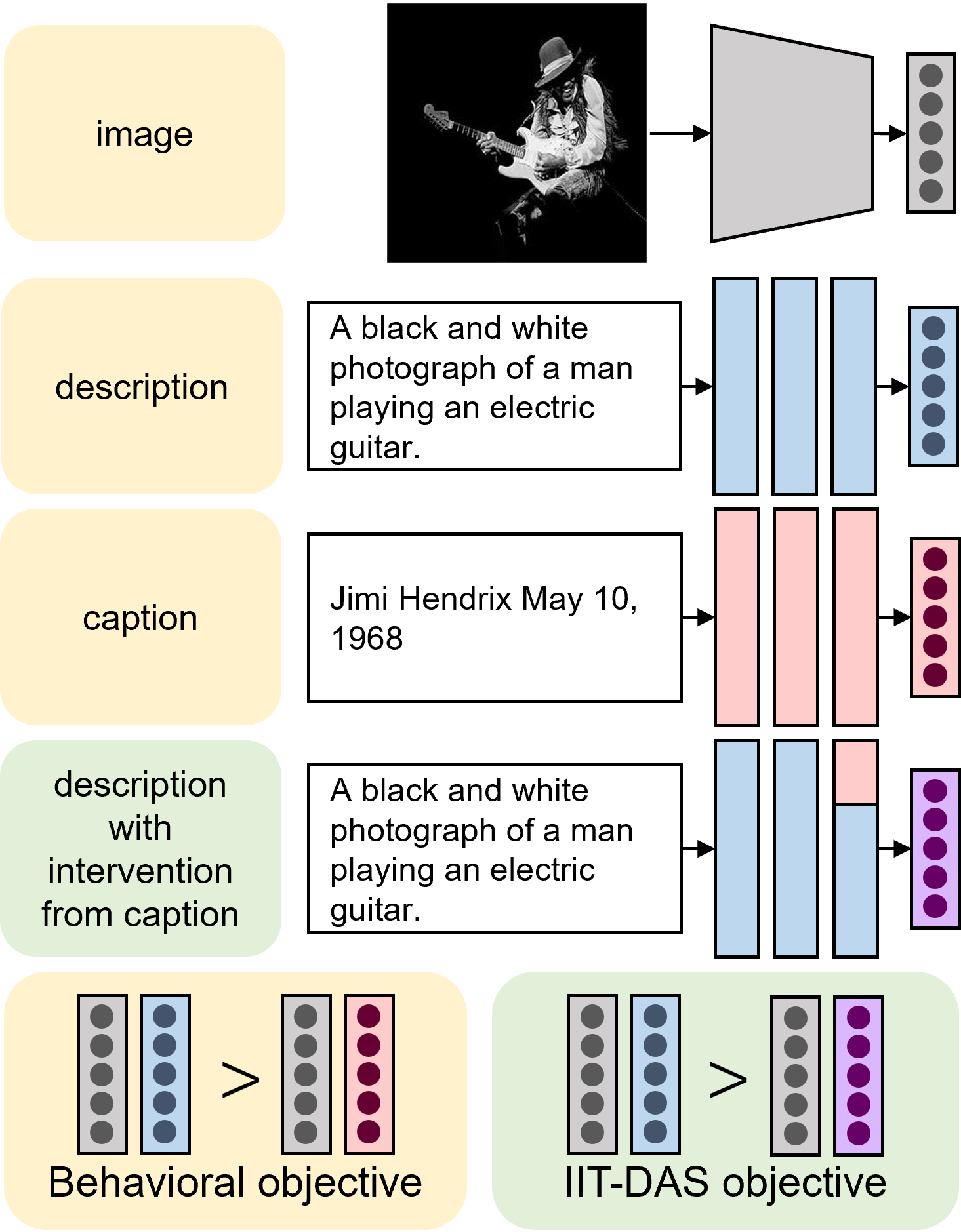
Figure 1: Visualization of a single training step on Concadia, updating CLIP to prefer descriptions to captions. Though both objectives update CLIP to be sensitive to the description–caption distinction, IIT-DAS localizes this distinction to a subspace of CLIP’s activations.

The Contrastive Language-Image Pre-training (CLIP) model of Radford et al. (2021) is an important case in point. CLIP is trained to embed images and texts with the objective of maximizing the similarity of related image–text pairs and minimizing the similarity of unrelated pairs, without reference to the purpose that the text accompanying an image plays.

The CLIPScore metric of (Hessel et al., 2021) inherits this limitation; CLIPScore is referenceless in that it makes no use of human-generated, ground-truth texts, but rather depends only on image–text pairs, and so it too is not sensitive to the purpose of the text. Indeed, Kreiss et al. (2022a) find that CLIPScores correlate with neither sighted nor BLV user evaluations of image alt-descriptions. Thus, despite high performance on many image–text classification tasks, CLIPScore is unsuitable for alt-text evaluation.

The goal of this paper is to update CLIP to assign higher scores to descriptions than captions when they are both relevant to an image, while preserving the model’s ability to select the most relevant text for a particular image. To this end, we fine-tune CLIP on the Concadia dataset (Kreiss et al., 2022b), which consists of 96,918 images with corresponding descriptions, captions, and textual context.

Our core goal in fine-tuning is to teach the model to prefer descriptions over captions. To this end, we use a contrastive loss objective, which updates CLIP to produce a higher score for the description than the caption of an image in Concadia. In addition, we propose an extension of this objective that seeks to amplify the core distinction and create more interpretable models. The guiding idea here is to use Concadia to approximate the counterfactual: What if the text for this image were a description instead of a caption (or vice versa)? These counterfactuals enable us to use a novel combination of two recent ideas from causal interpretability research: interchange intervention training (IIT; Geiger et al. 2022) with a distributed alignment search (DAS; Geiger et al. 2023b) to localize the description–caption concept to an activation vector.

Our experiments lead to a few key findings that have implications beyond the accessibility use case. First, we find that LoRA Hu et al. (2021) is superior to standard fine-tuning at raising the CLIPScore assigned to descriptions compared to captions while preserving the original capabilities of CLIP. Second, our analysis shows that improved performance on Concadia results in stronger correlations with BLV user judgements, affirming the value of our update. Third, we find that the IIT-DAS objective results in a more stable fine-tuning process. Fourth, the IIT-DAS objective produces a more interpretable model; to show this, we use mediated integrated gradients (Sundararajan et al., 2017; Wu et al., 2023) to characterize how the description–caption distinction is computed in our fine-tuned models. The key role of the IIT-DAS objective in these results illustrates one way that interpretability research can lead directly to more performant and understandable models.

	Fine-	Desc > Cap	Transfer tasks (F1 Score)			BLV user eval (Corr.)
Objective	tuning	Concadia	Food101	ImageNet	CIFAR100	Overall	Imaginability
None	None	49.4%	76.4%	53.6%	61.5%	0.08	0.10
Behavioral	Full	90.1% $\pm$ 0.73	27.8% $\pm$ 24.96	14.6% $\pm$ 13.47	30.9% $\pm$ 24.97	0.29 $\pm$ 0.17	0.31 $\pm$ 0.19
	LoRA	90.3% $\pm$ 0.72	64.4% $\pm$ 08.32	42.2% $\pm$ 06.98	55.6% $\pm$ 02.53	0.36 $\pm$ 0.10	0.38 $\pm$ 0.12
IIT-DAS	Full	88.9% $\pm$ 0.80	35.1% $\pm$ 16.35	19.5% $\pm$ 06.77	42.8% $\pm$ 09.85	0.24 $\pm$ 0.14	0.32 $\pm$ 0.17
	LoRA	86.6% $\pm$ 0.84	73.6% $\pm$ 03.22	45.1% $\pm$ 03.96	53.7% $\pm$ 03.80	0.19 $\pm$ 0.15	0.27 $\pm$ 0.15

Table 1: The percent of Concadia examples where descriptions are scored higher than captions (column 3), F1 scores on transfer learning tasks (columns 4-6), and correlation between BLV human preferences Kreiss et al. (2022a) and model similarity scores (columns 7, 8). The error bounds are 95% confidence intervals from 5 random seeds. Fine-tuning on Concadia produces models that better correlate with BLV preferences, LoRA is essential for preserving transfer learning, and IIT-DAS sacrifices a modest amount on Desc > Cap for better transfer learning.

2 Related Work

Image Accessibility

When images can’t be seen, visual descriptions of those images make them accessible. For images online, these descriptions can be provided in the HTML’s alt tag, which are then visually displayed if the image cannot be loaded or are read out by a screen reader to, for instance, users who are blind or low-vision (BLV). However, alt descriptions online remain rare Gleason et al. (2019); Kreiss et al. (2022b).

Image captioning models provide an opportunity to generate such accessibility descriptions at scale, which would promote equal access Gleason et al. (2020). But the resulting models have remained largely unsuccessful in practice Morris et al. (2016); MacLeod et al. (2017); Gleason et al. (2019). Kreiss et al. (2022b) argue that this is partly due to the general approach of treating all image-based text generation problems as the same underlying task, and instead highlight the need for a distinction between accessibility descriptions and contextualizing captions. Descriptions are needed to replace images, while the purpose of a caption is to provide supplemental information. Kreiss et al. (2022b) find that the language used in descriptions and captions categorically differs and that sighted participants tend to learn more from captions but can visualize the image better from descriptions.

Referenceless Text-Image Evaluation Metrics

We focus on referenceless evaluation metrics Feinglass and Yang (2021); Hessel et al. (2021); Lee et al. (2021) for text–image models. These can be applied in diverse contexts and require no human annotations, which makes them valuable tools for rapid system assessment. Crucially, such referenceless metrics are context-free. This brings the advantage that they can be applied in a variety of multimodal settings (e.g. image synthesis, description generation, zero-shot image classification). The downside is that they are generally insensitive to variation in context and purpose. Kreiss et al. (2022a, 2023) report progress in incorporating context into these metrics; our work can be seen as complementing those efforts by focusing on textual purpose.

3 Methods

Our goal is to fine-tune a CLIP model $\mathcal{C}^{\theta}$ to prefer a description over a caption when the two texts are relevant to an image, while preserving $\mathcal{C}^{\theta}$’s ability to select the most relevant text for a particular image. To this end, we use Concadia, a dataset that consists of $(x_{\text{image}},x_{\text{description}},x_{\text{caption}})$ triplets. We consider two different contrastive learning objectives and two common fine-tuning methods that minimally update $\mathcal{C}^{\theta}$’s sensitivity to the description–caption distinction.

Behavioral Objective

For each triplet $(x_{\text{im}},x_{\text{des}},x_{\text{cap}})$, we run $\mathcal{C}^{\theta}$ on the image–caption pair $(x_{\text{im}},x_{\text{cap}})$ and on the image–description pair $(x_{\text{im}},x_{\text{des}})$, and update $\mathcal{C}^{\theta}$ to produce a higher score for the latter by minimizing:

$$\mathcal{L}=\texttt{CE}\big{(}[\mathcal{C}^{\theta}(x_{\text{im}},x_{\text{cap}}),\mathcal{C}^{\theta}(x_{\text{im}},x_{\text{des}})],[0,1]\big{)}$$

IIT-DAS Objective

To better maintain CLIP’s original capabilities, we propose a novel objective called IIT-DAS, which localizes the description–caption distinction in a linear subspace $\mathbf{Z}$ of an activation vector in $\mathcal{C}^{\theta}$. For each triplet, we run $\mathcal{C}^{\theta}$ on the image-caption pair $(x_{\text{im}},x_{\text{cap}})$, run $\mathcal{C}^{\theta}$ on the image-caption pair again while fixing $\mathbf{Z}$ to the value it takes when $\mathcal{C}^{\theta}$ is run on the image description pair $(x_{\text{im}},x_{\text{des}})$, and update $\mathcal{C}^{\theta}$ to produce a higher score for the latter by minimizing:

$$\mathcal{L}_{\text{IIT}}=\texttt{CE}\big{(}[\mathcal{C}^{\theta}(x_{\text{im}},x_{\text{cap}}),\\ \textsc{DII}(\mathcal{C}^{\theta},\rho^{\theta},(x_{\text{im}},x_{\text{cap}}),(x_{\text{im}},x_{\text{des}}),\mathbf{Z})],[0,1]\big{)}$$

where $\rho^{\theta}$ is a randomly initialized orthogonal matrix used to learn the linear subspace $\mathbf{Z}$. This pushes CLIP to assign a higher score to a caption with an intervention from a description than to a caption on its own. Likewise, we also train on the objective where descriptions and captions are swapped (prefer a description over a description with an intervention from a caption):

$$\mathcal{L}_{\text{IIT}}=\texttt{CE}\big{(}[\mathcal{C}^{\theta}(x_{\text{im}},x_{\text{des}}),\\ \textsc{DII}(\mathcal{C}^{\theta},\rho^{\theta},(x_{\text{im}},x_{\text{des}}),(x_{\text{im}},x_{\text{cap}}),\mathbf{Z})],[1,0]\big{)}$$

See Appendix A for the formal definition of DII.

Fine-tuning

We consider two common fine-tuning methods that update CLIP in accordance with the selected objective. The first is full fine-tuning where all the parameters of CLIP are trained with gradient descent. The second is Low-Rank Adaptation (LoRA), a state-of-the-art fine-tuning technique for transfer learning Hu et al. (2021). LoRA training freezes every linear layer $W$ in a model and learns a low-rank matrix $W^{\prime}$ that is used in unison with the original weights (i.e. for a residual representation $x$, LoRA computes $Wx+W^{\prime}x$).

4 Experiments

4.1 Concadia and Transfer Evaluations

We use Concadia to quantify the extent to which an image–text model is sensitive to the description–caption distinction. The metric is simply the proportion of images in Concadia where the description is assigned a higher score than the caption. In the pre-trained CLIP model, this is the case for $\approx$50% of the triplets in Concadia (see Table 1). This means the model assigns higher scores to descriptions only at chance and so is not well suited for the purposes of accessibility. However, we also need to evaluate to what extent each fine-tuning method preserves the original transfer capabilities of CLIP. The ideal method will maintain high performance on the image classification transfer tasks, while preferring descriptions over captions.

We evaluate our fine-tuned models on Concadia and three image classification tasks in disparate domains, selected from CLIP’s original evaluation suite Radford et al. (2021) (see Appendix C).

Results and Discussion

Table 1 shows the performance of each CLIP model on the Concadia and transfer evaluations. Full fine-tuning is not viable due to its poor performance on the transfer learning tasks. LoRA helps preserve much of the original model’s capabilities (dropping $\approx$10% on Food101 and Imagenet, and $\approx$6% on CIFAR).

The models trained on the behavioral objective are more sensitive to the description–caption distinction ($\approx$90%) than IIT-DAS with LoRA ($\approx$87%). In contrast, models trained on the IIT-DAS objective with LoRA achieve the best performance on transfer tasks (preserving CLIP’s original Food101 accuracy within its 95% confidence interval), though sacrificing some sensitivity to the description–caption distinction ($\approx$86%). The IIT-DAS objective is comparable to the behavioral objective; either one may be preferable depending on the desired balance between description–caption sensitivity and transfer capabilities.

4.2 BLV and Sighted Human Evaluations

A preference for descriptions over captions should align CLIPScore ratings better with the quality judgements of BLV and sighted individuals. To evaluate this, we use data from Kreiss et al. 2022a. Kreiss et al. conducted an experiment where sighted and BLV participants were asked to judge a text describing an image in the context of an article (See Appendix D for experimental details). For our purposes, we ignore the context and isolate the benefit of descriptions compared to captions. Participants rated the quality of the image descriptions along four dimensions: the overall quality of the text for accessibility, the imaginability of the image just based on the text, and the degree of relevant and irrelevant details in the text.

Results and Discussion

For each model evaluated, we report correlations averaged across 5 runs. Table 1 shows the correlation between BLV individuals’ preferences and model similarity scores for the overall and imaginability dimensions (see Appendix D for all dimensions and subject groups).

Our results show clearly that fine-tuning CLIP on the Concadia dataset results in a CLIPScore that is better aligned with the judgments of BLV individuals. This agrees with the finding that the description–caption distinction is important for BLV users Kreiss et al. (2022a).

A broad trend is that the more a model is able to distinguish between descriptions and captions the more it aligns with the judgements of BLV individuals. As such, the models trained on the behavioral objective have the highest correlations.

Example	Mediation	Attribution
Desc.	✗	ablackandwhitephotographofjimihendrix
		playingafenderstratocasterelectricguitar
	✓	ablackandwhitephotographofjimihendrix
		playingafenderstratocasterelectricguitar
Caption	✗	jimihendrix,fillmoreeast,may10,1968
	✓	jimihendrix,fillmoreeast,may10,1968

Figure 2: Integrated gradient attributions for the IIT-DAS model run on an image and its corresponding description and caption from the Concadia dataset. A positive token attribution indicates a positive impact on CLIPScore (green), and negative token attribution indicates a negative impact (magenta).

4.3 Integrated Gradients

A key benefit of localizing the description–caption distinction in CLIP with IIT-DAS is that we can interpret CLIP’s representation of a text’s communicative purpose (description or caption) separately from CLIP’s similarity score. In this section, we conduct an analysis of how CLIP distinguishes between descriptions and captions using an attribution method called integrated gradients (IG; Sundararajan et al. 2017) that evaluates the contribution of each text token to the output CLIPScore.

We are particularly curious about how tokens impact the representation of the description–caption distinction. To answer this question, we mediate the gradient computation through the linear subspace learned by IIT-DAS Wu et al. (2023). We hypothesize that, since the intervention site is trained to represent the underlying purpose of a text (i.e. description or caption), gradient attributions that are mediated through the linear subspace learned by IIT-DAS will pick out tokens that highlight the description–caption distinction.

Figure 2 shows an example image from Concadia and the IG attributions of its corresponding description and caption on the IIT-DAS model. We observe that although the overall attributions are positive for the guitarist’s name (“Jimi Hendrix”), the mediated attributions for these tokens are negative. While “Jimi Hendrix” is aligned with the image (high overall), proper names are less likely to appear in descriptions (low mediated).

We hypothesize that the interpretability afforded by mediated IG attributions will align with the distinct purposes behind describing and captioning images. Specifically, descriptions are easier to visualize than captions, since their goal is to supplant the image’s visual components as opposed to supplement them Kreiss et al. (2022b). Hence, we expect that words with higher attributions are easier to visualize. And, indeed, we find that mediated IG attributions for CLIP trained with IIT-DAS correlate with human ratings for imageability and concreteness, whereas IG attributions for the original CLIP model do not. See Appendix E for more details on mediated IG as well as imageability and concreteness correlations.

5 Conclusion

We update the CLIP model to prefer descriptions over captions using Concadia and produce a useful, accessible, and interpretable model.

Limitations

Our results serve as proof concept for using IIT-DAS to update CLIP with the Concadia dataset. This is one model and one dataset, so general conclusions about the use of IIT-DAS for updating a pretrained model should not be drawn. We hope future work will shed further light on the value of IIT-DAS.

The Concadia dataset provides textual context for each image-description-caption triple. We do not use the context in our experiments, but we are excited about future work that incorporates this data. Whereas our work focuses on the specific purposes of describing and captioning an image, the context of an image can illuminate many other purposes (e.g. search, geolocation, social communication) and models that incorporate it can enrich our work.

Ethics Statement

We believe that modern AI is a transformative technology that should benefit all of us and accessibility applications are an important part of this.

Appendix A Causal Models, Interchange Intervention Training, and Distributed Alignment Search

This section follows Geiger et al. 2023a, b.

Causal Models can represent a variety of processes, including deep learning models and symbolic algorithms. A causal model $\mathcal{M}$ consist of variables $\mathbf{V}$, and, for each variable $X\in\mathbf{V}$, a set of values $\texttt{Val}(X)$, and a structural equation $F_{X}:\texttt{Val}(\mathbf{V})\to\texttt{Val}(X)$, which is a function that takes in a setting of all the variables and outputs a value for $X$. The solutions of a model $\mathcal{M}=(\mathbf{V},\texttt{Val},F)$ are settings for all variables $\mathbf{v}\in\texttt{Val}(\mathbf{V})$ such that the output of the causal mechanism $F_{X}(\mathbf{v})$ is the same value that $\mathbf{v}$ assigns to $X$, for each $X\in\mathbf{V}$.

We only consider structural causal models with a single solution that induces a directed acyclic graphical structure such that the value for a variable $X$ depends only on the set of variables that point to it, denoted as its parents $\emph{PA}_{X}$. Because of this, we treat each causal mechanism $F_{X}$ as a function from parent values in $\texttt{Val}(\emph{PA}_{X})$ to a value in $\texttt{Val}(X)$. We denote the set of variables with no parents as $\mathbf{V}_{\emph{in}}$ and those with no children $\mathbf{V}_{\emph{out}}$.

Given $\mathsf{input}\in\texttt{Val}(\mathbf{V}_{\emph{in}}$) and variables $\mathbf{X}\subseteq\mathbf{V}$, we define $\texttt{GET}(\mathcal{M},\mathsf{input},\mathbf{X})\in\texttt{Val}(\mathbf{X})$ to be the setting of $\mathbf{X}$ determined by the given $\mathsf{input}$ and model $\mathcal{M}$. For example, $\mathbf{X}$ could correspond to a hidden activation layer in a neural network, and $\texttt{GET}(\mathcal{M},\mathsf{input},\mathbf{X})$ then denotes the particular values that $\mathbf{X}$ takes on when the model $\mathcal{M}$ processes $\mathsf{input}$.

Interventions simulate counterfactual states in causal models. For a set of variables $\mathbf{X}$ and a setting for those variables $\mathbf{x}\in\texttt{VAL}(\mathbf{X})$, we define $\mathcal{M}_{\mathbf{X}\leftarrow\mathbf{x}}$ to be the causal model identical to $\mathcal{M}$, except that the structural equations for $\mathbf{X}$ are set to constant values $\mathbf{x}$. In the case of neural networks, we overwrite the activations with $\mathbf{x}$ in-place so that gradients can back-propagate through $\mathbf{x}$.

Distributed interventions also simulate counterfactual states in causal models, but do so by editing the causal mechanisms rather than overwriting them to be a constant. Given variables $\mathbf{X}$ and an invertible function $\rho:\texttt{VAL}(\mathbf{X})\to\texttt{VAL}(\mathbf{Y})$ mapping $\mathbf{X}$ into a new variable space $\mathbf{Y}$, define $\rho(\mathcal{M})$ to be the model where the variables $\mathbf{X}$ are replaced with the variables $\mathbf{Y}$. For a setting of the new variable space $\mathbf{y}\in\texttt{VAL}(\mathbf{Y})$, it follows that $\rho^{-1}(\rho(\mathcal{M})_{\mathbf{Y}\leftarrow\mathbf{y}})$ is the causal model identical to $\mathcal{M}$, except that the causal mechanisms for $\mathbf{X}$ are edited to fix the value of $\mathbf{Y}$ to $\mathbf{y}$. If $\rho$ is differentiable, then gradients back-propagate through $\mathbf{y}$.

A distributed interchange intervention fixes variables to the values they would have taken if a different input were provided. Consider a causal model $\mathcal{M}$, an invertible function $\rho:\texttt{VAL}(\mathbf{X})\to\texttt{VAL}(\mathbf{Y})$, source and base inputs $\mathbf{s},\mathbf{b}\in\texttt{Val}(\mathbf{V}_{\emph{in}})$, and a set of intermediate variables $\mathbf{X}\subset\mathbf{V}$. A distributed interchange intervention computes the value $\mathbf{V}_{\emph{out}}$ when run on $\mathbf{b}$, intervening on the (distributed) intermediate variables $\mathbf{Y}$ to be the value they take on when run on $\mathbf{s}$. Formally, we define

$$\textsc{DII}(\mathcal{M},\rho,\mathbf{b},\mathbf{s},\mathbf{Y})=\\ \texttt{GET}(\rho^{-1}(\rho(\mathcal{M})_{\mathbf{Y}\leftarrow\texttt{GET}(\rho(\mathcal{M}),\mathbf{s},\mathbf{Y})}),\mathbf{b},\mathbf{V}_{\emph{out}})$$

High-Level Models

Define a class $\Delta$ to contain only causal models that consist of the following three variables. The input variable $X$ takes on the value of some image-text pair in Concadia $(x_{\text{image}},x_{\text{text}})$; the intermediate variable $P$ (i.e. purpose) takes on a value from $\{\text{``describe''},\text{``caption''}\}$ depending on the Concadia label for $X$; and the output variable $Y$ takes on a real value that represents the similarity between $x_{\text{image}}$ and $x_{\text{text}}$. The causal mechanism of $Y$ must be such that for every image, the description text is assigned a higher CLIPScore than the caption text. If a CLIP model implements any algorithm in $\Delta$, then it will assign descriptions higher scores than captions.

Appendix B Training Details

In this paper, we propose a novel combination of LoRA fine-tuning with the IIT-DAS objective. We apply DAS to the representation after LoRA is applied (i.e., $Wx+W^{\prime}x$, where $W$ is the original matrix weight and $W^{\prime}$ is the low-rank adaptation), and fine-tune the LoRA parameters $W^{\prime}$ and the rotation matrix $\rho^{\theta}$.

We fine-tune the CLIP ViT-B/32 Transformer model released by OpenAI, which consists of 12 transformer layers with a hidden dimension of 512, constituting $\sim$150M overall parameters. For all fine-tuning runs, we use Adam optimization with default parameters Kingma and Ba (2014) and a batch size of 12.

Behavioral Objective

We fine-tune CLIP on the training split of the Concadia dataset (77,534 datapoints) with early-stopping validation on the Concadia validation split (9,693 datapoints). We conduct a hyperparameter grid search over a learning rate $\emph{lr}\in\{10^{-3},0.5\cdot 10^{-3},10^{-4},0.5\cdot 10^{-4},\ldots,10^{-6},0.5\cdot 10^{-6}\}$, an L2 normalization factor $\emph{l}_{2}\in\{0,0.1,0.01,0.001\}$. We select the configuration with the highest accuracy on the Concadia validation split within 5 epochs ($\emph{lr}=0.5\cdot 10^{-6}$, $\emph{l}_{2}=0$). A training run takes around 3 hours on an RTX A6000 NVIDIA GPU.

IIT-DAS Objective

We fine-tune CLIP on 100,000 triplets sampled from the train split of the Concadia dataset (out of $77,534\times 77,534$ possible caption–description pairs). We conduct a hyperparameter grid search over a learning rate $\emph{lr}\in\{10^{-5},5^{-6},10^{-6}\}$, as well as over the intervention site: the layer $\emph{layer}\in\{6,8,10\}$, the intervention site size $\emph{intervention-size}\in\{32,64,128,256\}$. We select the configuration with the highest accuracy on the Concadia validation split within 5 epochs ($\emph{lr}=10^{-5},\emph{layer}=10,\emph{intervention-size}=256$). A training run takes around 6 hours on an RTX A6000 NVIDIA GPU.

LoRA Fine-Tuning

We perform an additional hyperparameter search for low-rank fine-tuning of CLIP for both the behavioral and IIT-DAS objective. We take the best configuration for full-finetuning, and then perform a search over the LoRA rank $\emph{rank}\in\{8,16,32,64,128\}$, the LoRA dropout $\emph{dropout}\in\{0,0.1,0.01\}$, and whether to apply LoRA to all linear layers, all attention weights, or only the query and value projection matrices within attention weights. We select the configuration with the highest accuracy on the Concadia validation split with 5 epochs. For the behavioral objective, the configuration is $\emph{rank}=64$, $\emph{dropout}=0$, with LoRA applied to all attention weights. For the IIT-DAS objective, the configuration is the same but with $\emph{rank}=128$.

Joint Objective

We note that the behavioral objective and IIT-DAS objective can complement each other – the former teaches the model to prefer descriptions to captions, and the latter teaches the model to localize this distinction in a particular representation. Hence, we consider a joint objective, where we train the model to minimize

$$\mathcal{L}_{\text{Joint}}=\alpha\mathcal{L}_{\text{IIT}}+(1-\alpha)\mathcal{L}_{\text{Behavioral}}$$

We search over an interpolation factor $\alpha\in\{0.2,0.3,0.5,0.7,0.8\}$. However, we find that the joint objective neither improves upon the behavioral objective nor the IIT-DAS objective.

Appendix C Transfer Evaluations

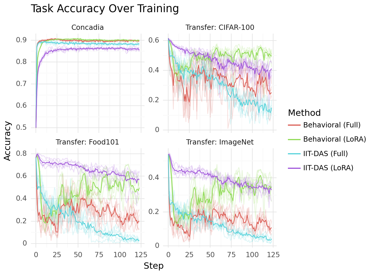
Figure 3: Accuracy on the Concadia test set, and the three transfer tasks selected for transfer evaluation (CIFAR-100, Food101, and ImageNet).

We evaluate our fine-tuned CLIP models on tasks selected from the original suite of zero-shot evaluations performed on CLIP Radford et al. (2021). Specifically, we choose three zero-shot image classification tasks in which CLIP has strong performance, described briefly below.

CIFAR-100

Images from 100 different categories Krizhevsky et al. (2009).

Food101

Food images labeled from 101 categories Bossard et al. (2014).

ImageNet

Image-text pairs for each synonym set in the WordNet hierarchy Russakovsky et al. (2015); Miller (1995).

Pre-trained CLIP varies greatly in its ability to generalize to each of these tasks, but it does outperform a supervised linear classifier trained on ResNet-50 features Radford et al. (2021). We report the macro-averaged F1 score on zero-shot classification for each of the transfer tasks listed above, averaged across 5 randomly seeded training runs. During evaluation, we prefix “An image of ___” to each label in order to improve zero-shot generalization.

Figure 3 shows model accuracy throughout training for the 5 randomly seeded training runs of each training objective and fine-tuning method. Although the training converges quickly on the Concadia dataset, training for longer seems to allow the model to recover performance on the evaluated transfer tasks when using LoRA fine-tuning. Hence, for the evaluation scores reported in Table 1, we train models well past convergence for 10 epochs, and then select a model to balance the trade-off between Concadia accuracy and transfer capabilities:

• Compute a recovery percentage: divide the model’s accuracy on the transfer task by the accuracy of pre-trained CLIP on that task (see Table 1).

• Compute a transfer score: average the recovery percentage across the three transfer tasks.

• Compute accuracy–transfer trade-off score: compute $\alpha\cdot$ (Concadia accuracy) $+(1-\alpha)\cdot$ (transfer score).

• For each seeded run, select the training step with the highest accuracy–transfer trade-off score.

Figure 4: Transfer score (averaged recovery percentage over all transfer tasks) over accuracy on the Concadia test set. A point on a seeded run yields a trade-off between sensitivity to the caption–description distinction and preserving the capabilities of CLIP. The joint objective refers to a training run minimizing both the behavioral and the IIT-DAS objective (see Appendix B).

We manually pick a trade-off of $\alpha=0.9$, meaning we weigh the trade-off as 90% Concadia accuracy and 10% transfer accuracy; we find that trade-offs with a lower $\alpha$ result in poor Concadia accuracy.

We visualize other possible trade-off in Figure 4. We find that the strongest trade-off for IIT-DAS with LoRA fine-tuning is $\approx 86\%$ accuracy on the Concadia test set and $\approx 82\%$ transfer score. Meanwhile, the strongest trade-off for the behavioral objective with LoRA fine-tuning is skewed towards stronger Concadia performance, with $\approx 90\%$ accuracy on Concadia and $\approx 80\%$ transfer score.

Figure 4 also displays the transfer–accuracy trade-off for a joint objective that minimizes both the behavioral and the IIT-DAS objective (see Appendix B for details). The joint objective seems to strike some balance between the trade-off curves of the behavioral and IIT-DAS objectives – maintaining higher transfer scores around $\approx 85\%$ Concadia accuracy compared to the behavioral objective, and reaching higher Concadia accuracy ($\approx 90\%$) compared to IIT-DAS. Nevertheless, for any given Concadia accuracy value, one of the behavioral or IIT-DAS objectives achieves at least as high a transfer score as the joint objective. We leave strategies to optimally combine the behavioral and IIT-DAS objectives for further study.

Appendix D BLV and Sighted Evaluations

Table 2 reports the correlation between fine-tuned CLIPScoresand human evaluations collected by Kreiss et al. (2022a). The evaluations are from BLV individuals, sighted individuals without access to the image the text describes, and sighted individuals with access to the image. The evaluation features are briefly summarized below.

Overall

The overall value of the description as an alt-text description of the image.

Imaginability

How well the participant can visualize the image given the text description. This isn’t evaluated for sighted individuals with the image, since they are able to see the reference image.

Relevance

Whether the description includes relevant details from the image, given the context in which the image appears (i.e., the preceding paragraph in a Wikipedia article).

Irrelevance

Whether the description avoids irrelevant details from the image, given the context of in which the image appears.

Kreiss et al. (2022a) recruited 16 participants via email lists for BLV users that were unaware of the studies purpose. Participants were totally blind (7), nearly blind (3), light perception only (5), and low vision (1). 15 participants reported relying on screen readers (almost) always when browsing the Web, and one reported using them often. In total, judgements were provided for 68 descriptions, comprising 18 images and 17 Wikipedia articles.

We find that fine-tuning CLIP on the Concadia dataset improves the model’s correlation with human judgements of text descriptions. We note that fine-tuning CLIP does not significantly improve the model’s correlation with human judgements of irrelevant details in the text description. This makes sense, because our training scheme did not take into account to the context of the Concadia image.

Group	Objective	Finetuning	Overall	Imaginability	Relevance	Irrelevance
BLV	None	None	0.08	0.10	0.09	0.09
	Behavioral	Full	0.24$\pm$ 0.04	0.26$\pm$ 0.03	0.21$\pm$ 0.04	0.05$\pm$ 0.09
		LoRA	0.29$\pm$ 0.03	0.29$\pm$ 0.01	0.23$\pm$ 0.02	-0.01$\pm$ 0.03
	IIT-DAS	Full	0.29$\pm$ 0.05	0.34$\pm$ 0.05	0.30$\pm$ 0.06	0.07$\pm$ 0.05
		LoRA	0.20$\pm$ 0.09	0.28$\pm$ 0.10	0.24$\pm$ 0.07	0.01$\pm$ 0.06
Sighted	None	None	$-$0.01	0.06	0.00	$-$0.17
(no image)	Behavioral	Full	0.22$\pm$ 0.04	0.13$\pm$ 0.09	0.17$\pm$ 0.03	-0.03$\pm$ 0.03
		LoRA	0.20$\pm$ 0.02	0.20$\pm$ 0.04	0.18$\pm$ 0.02	-0.13$\pm$ 0.05
	IIT-DAS	Full	0.18$\pm$ 0.06	0.21$\pm$ 0.03	0.12$\pm$ 0.08	-0.14$\pm$ 0.06
		LoRA	0.13$\pm$ 0.05	0.18$\pm$ 0.04	0.11$\pm$ 0.05	-0.09$\pm$ 0.06
Sighted	None	None	0.14		0.11	$-$0.08
(with image)	Behavioral	Full	0.26$\pm$ 0.05		0.22$\pm$ 0.04	0.03$\pm$ 0.05
		LoRA	0.25$\pm$ 0.02		0.19$\pm$ 0.02	-0.04$\pm$ 0.04
	IIT-DAS	Full	0.25$\pm$ 0.06		0.17$\pm$ 0.07	-0.04$\pm$ 0.07
		LoRA	0.22$\pm$ 0.06		0.15$\pm$ 0.05	0.02$\pm$ 0.06

Table 2: Correlation between model similarity scores and human preferences Kreiss et al. (2022a).

Example	Mediation	Score	Attribution
Description	✗	+12.0	aclusterofpurplish-redmushroomsontheirsidesshowingtheundersideoftheircaps.
	✓	+5.77	aclusterofpurplish-redmushroomsontheirsidesshowingtheundersideoftheircaps.
Caption	✗	-2.95	youngfruitbodiesarepruinoseasifcoveredwithafinewhitepowder.
	✓	-2.99	youngfruitbodiesarepruinoseasifcoveredwithafinewhitepowder.

Example	Mediation	Score	Attribution
Description	✗	+1.35	ablockofflatsbehindasetofhighsecuritygates
	✓	-1.38	ablockofflatsbehindasetofhighsecuritygates
Caption	✗	-7.85	theexclusiveblockofflatsinchelsea,londonthatwereusedastheexteriorofmark’sflat
	✓	-9.15	theexclusiveblockofflatsinchelsea,londonthatwereusedastheexteriorofmark’sflat

Figure 5: Integrated gradient attributions for sample images and their corresponding description and caption from the Concadia dataset. A positive token attribution means that the token contributed positively to the outputted CLIPScore (green), and negative token attribution means that it contributed negatively (magenta). The overall score is the sum of the token attributions within the sentence.

Appendix E Integrated Gradients

Given a model $\mathcal{C}^{\theta}$ with input $x$ and baseline $x^{\prime}$, the integrated gradient attributions of $x$ along its $i$th dimension are computed as follows.

$$\texttt{IntegratedGrads}_{i}(x)=(x_{i}-x^{\prime}_{i})\cdot\\ \int_{\alpha=0}^{1}\frac{\partial\mathcal{C}^{\theta}(x^{\prime}+\alpha(x-x^{\prime}))}{\partial x_{i}}\ \partial\alpha.$$ (1)

Mediated Integrated Gradients

Let $H$ be the activation of $\mathcal{C}^{\theta}$ at the intervention site when run on input $x$. Our mediated integrated gradient is

$$\frac{\partial\mathcal{C}^{\theta}}{\partial x_{i}}\text{ mediated by }H=\frac{\partial\mathcal{C}^{\theta}}{\partial H}\times\frac{\partial H}{\partial x_{i}}.$$

Unlike $\frac{\partial\mathcal{C}^{\theta}}{\partial x_{i}}$, which computes the gradient of the model output with respect to the input $x_{i}$, the mediated gradient only flows through the intervention site $H$. We compute mediated integrated gradients by applying this gradient method within the integral of the integrated gradients equation.

Figure 5 illustrates additional examples of integrated gradients and mediated gradients on images sampled from the Concadia dataset, run with the IIT-DAS model.

Dataset

We hypothesize that the interpretability afforded by mediated integrated gradients will align with the distinct purposes behind describing and captioning images. Specifically, descriptions are easier to visualize than captions, since their goal is to supplant the image’s visual components as opposed to supplement them Kreiss et al. (2022b). Hence, we expect that words with higher integrated gradient attributions are easier to visualize.

We consult two collections of human ratings for visualization-related concepts. The first dataset consists of 5,500 words rated by imageability, or how well a word evokes a clear mental image in the reader’s mind Scott et al. (2019). The second dataset consists of over 40,000 words rated by concreteness, or how clearly a word corresponds to a perceptible entity Brysbaert et al. (2014). We randomly sample 100 captions and 100 descriptions from the test split of the Concadia dataset that contain at least one word within both of our datasets, consisting of 420 unique tokens in total. We compute the integrated gradient attributions for all tokens in those sentences, and report their correlations with imageability and concreteness ratings.

Results

Table 3 displays the correlations between token-level attributions of the LoRA model output and human ratings for imageability and concreteness. All fine-tuning methods achieve a stronger correlation with imageability and concreteness ratings than the base CLIP model.

Although all fine-tuning methods result in mediated gradient attributions that correlate with imageability and concreteness, only the IIT and IIT-DAS attributions localize to the mediation site. The difference in mediating through vs. around the learned site is significant for the IIT-DAS model ($0.23\pm 0.03$ vs. $0.10\pm 0.09$ for concreteness, and $0.23\pm 0.03$ vs. $0.03\pm 0.09$ for imageability).

Discussion

Our results show that fine-tuning CLIP to prefer descriptions over captions with IIT or IIT-DAS results in models whose attributions correspond to the human-interpretable concept of imageability and concreteness. We also find that mediating integrated gradients through the representation targetted by IIT preserves this correlation and allows for an analysis of which tokens contribute to distinguishing descriptions from captions.

Training	Mediation	Concreteness	Imageability
None	None	0.20	0.16
	Through	0.14	0.07
	Around	-	-
Behavioral	None	$0.26\pm 0.08$	$0.31\pm 0.08$
	Through	$0.24\pm 0.08$	$0.24\pm 0.08$
	Around	$0.24\pm 0.02$	$0.30\pm 0.03$
IIT-DAS	None	$0.26\pm 0.08$	$0.23\pm 0.08$
	Through	$0.23\pm 0.03$	$0.23\pm 0.03$
	Around	$0.10\pm 0.09$	$0.03\pm 0.09$

Table 3: Correlation between integrated gradient attributions and per-token human labels for concreteness and imageability. The error bounds are 95% confidence intervals from runs with five random seeds.

References

- Bigham et al. (2006) Jeffrey P Bigham, Ryan S Kaminsky, Richard E Ladner, Oscar M Danielsson, and Gordon L Hempton. 2006. Webinsight: making web images accessible. In Proceedings of the 8th International ACM SIGACCESS Conference on Computers and Accessibility, pages 181–188.
- Bossard et al. (2014) Lukas Bossard, Matthieu Guillaumin, and Luc Van Gool. 2014. Food-101 – mining discriminative components with random forests. In European Conference on Computer Vision.
- Brysbaert et al. (2014) Marc Brysbaert, Amy Beth Warriner, and Victor Kuperman. 2014. Concreteness ratings for 40 thousand generally known english word lemmas. Behavior research methods, 46:904–911.
- Feinglass and Yang (2021) Joshua Feinglass and Yezhou Yang. 2021. Smurf: Semantic and linguistic understanding fusion for caption evaluation via typicality analysis. arXiv preprint arXiv:2106.01444.
- Geiger et al. (2023a) Atticus Geiger, Chris Potts, and Thomas Icard. 2023a. Causal abstraction for faithful model interpretation.
- Geiger et al. (2022) Atticus Geiger, Zhengxuan Wu, Hanson Lu, Josh Rozner, Elisa Kreiss, Thomas Icard, Noah Goodman, and Christopher Potts. 2022. Inducing causal structure for interpretable neural networks. In International Conference on Machine Learning, pages 7324–7338. PMLR.
- Geiger et al. (2023b) Atticus Geiger, Zhengxuan Wu, Christopher Potts, Thomas Icard, and Noah D. Goodman. 2023b. Finding alignments between interpretable causal variables and distributed neural representations.
- Gleason et al. (2019) Cole Gleason, Patrick Carrington, Cameron Cassidy, Meredith Ringel Morris, Kris M Kitani, and Jeffrey P Bigham. 2019. “it’s almost like they’re trying to hide it”: How user-provided image descriptions have failed to make twitter accessible. In The World Wide Web Conference, pages 549–559.
- Gleason et al. (2020) Cole Gleason, Amy Pavel, Emma McCamey, Christina Low, Patrick Carrington, Kris M Kitani, and Jeffrey P Bigham. 2020. Twitter a11y: A browser extension to make twitter images accessible. In Proceedings of the 2020 chi conference on human factors in computing systems, pages 1–12.
- Hessel et al. (2021) Jack Hessel, Ari Holtzman, Maxwell Forbes, Ronan Le Bras, and Yejin Choi. 2021. Clipscore: A reference-free evaluation metric for image captioning. CoRR, abs/2104.08718.
- Hu et al. (2021) Edward J Hu, Yelong Shen, Phillip Wallis, Zeyuan Allen-Zhu, Yuanzhi Li, Shean Wang, Lu Wang, and Weizhu Chen. 2021. Lora: Low-rank adaptation of large language models. arXiv preprint arXiv:2106.09685.
- Kingma and Ba (2014) Diederik P Kingma and Jimmy Ba. 2014. Adam: A method for stochastic optimization. arXiv preprint arXiv:1412.6980.
- Kreiss et al. (2022a) Elisa Kreiss, Cynthia Bennett, Shayan Hooshmand, Eric Zelikman, Meredith Ringel Morris, and Christopher Potts. 2022a. Context matters for image descriptions for accessibility: Challenges for referenceless evaluation metrics. In Proceedings of the 2022 Conference on Empirical Methods in Natural Language Processing, pages 4685–4697.
- Kreiss et al. (2022b) Elisa Kreiss, Fei Fang, Noah Goodman, and Christopher Potts. 2022b. Concadia: Towards image-based text generation with a purpose. In Proceedings of the 2022 Conference on Empirical Methods in Natural Language Processing, pages 4667–4684.
- Kreiss et al. (2023) Elisa Kreiss, Eric Zelikman, Christopher Potts, and Nick Haber. 2023. ContextRef: Evaluating referenceless metrics for image description generation. Ms., Stanford University.
- Krizhevsky et al. (2009) Alex Krizhevsky, Geoffrey Hinton, et al. 2009. Learning multiple layers of features from tiny images.
- Lee et al. (2021) Hwanhee Lee, Seunghyun Yoon, Franck Dernoncourt, Trung Bui, and Kyomin Jung. 2021. Umic: An unreferenced metric for image captioning via contrastive learning. arXiv preprint arXiv:2106.14019.
- MacLeod et al. (2017) Haley MacLeod, Cynthia L Bennett, Meredith Ringel Morris, and Edward Cutrell. 2017. Understanding blind people’s experiences with computer-generated captions of social media images. In proceedings of the 2017 CHI conference on human factors in computing systems, pages 5988–5999.
- Miller (1995) George A Miller. 1995. Wordnet: a lexical database for english. Communications of the ACM, 38(11):39–41.
- Morris et al. (2016) Meredith Ringel Morris, Annuska Zolyomi, Catherine Yao, Sina Bahram, Jeffrey P Bigham, and Shaun K Kane. 2016. " with most of it being pictures now, i rarely use it" understanding twitter’s evolving accessibility to blind users. In Proceedings of the 2016 CHI conference on human factors in computing systems, pages 5506–5516.
- Radford et al. (2021) Alec Radford, Jong Wook Kim, Chris Hallacy, Aditya Ramesh, Gabriel Goh, Sandhini Agarwal, Girish Sastry, Amanda Askell, Pamela Mishkin, Jack Clark, Gretchen Krueger, and Ilya Sutskever. 2021. Learning transferable visual models from natural language supervision. In Proceedings of the 38th International Conference on Machine Learning, ICML 2021, 18-24 July 2021, Virtual Event, volume 139 of Proceedings of Machine Learning Research, pages 8748–8763. PMLR.
- Russakovsky et al. (2015) Olga Russakovsky, Jia Deng, Hao Su, Jonathan Krause, Sanjeev Satheesh, Sean Ma, Zhiheng Huang, Andrej Karpathy, Aditya Khosla, Michael Bernstein, Alexander C. Berg, and Li Fei-Fei. 2015. ImageNet Large Scale Visual Recognition Challenge. International Journal of Computer Vision (IJCV), 115(3):211–252.
- Scott et al. (2019) Graham G Scott, Anne Keitel, Marc Becirspahic, Bo Yao, and Sara C Sereno. 2019. The glasgow norms: Ratings of 5,500 words on nine scales. Behavior research methods, 51:1258–1270.
- Sundararajan et al. (2017) Mukund Sundararajan, Ankur Taly, and Qiqi Yan. 2017. Axiomatic attribution for deep networks. In International conference on machine learning, pages 3319–3328. PMLR.
- Wu et al. (2023) Zhengxuan Wu, Karel D’Oosterlinck, Atticus Geiger, Amir Zur, and Christopher Potts. 2023. Causal proxy models for concept-based model explanations. In International Conference on Machine Learning, pages 37313–37334. PMLR.