Grover’s algorithm on two-way quantum computer
Abstract
Two-way quantum computing (2WQC) represents a novel approach to quantum computing that introduces a CPT version of state preparation. This paper analyses the influence of this approach on Grover’s algorithm and compares the behaviour of typical Grover and its 2WQC version in the presence of noise in the system. Our findings indicate that, in an ideal scenario without noise, the 2WQC Grover algorithm exhibits a constant complexity of . In the presence of noise, the 2WQC Grover algorithm demonstrates greater resilience to different noise models than the standard Grover’s algorithm.
I Two-way quantum computers
Standard one-way quantum computers (1WQC) evolve the state of a quantum register over time in a specific direction. The initial state is under control, but the final state is random. As pairs of actions such as pull/push, negative/positive pressure, stimulated emission/absorption causing deexcitation/excitation are CPT analogs, and the former can be used for state preparation, the latter should allow for its CPT analog, referred to here as CPT(state preparation), which allows for additional chosen enforcement of the final state, and thus represents a more active treatment than measurement. This allows the construction of two-way quantum computers [1] (2WQC), which are capable of more efficiently addressing NP problems by concurrently managing the flow of information.
II Traditional Grover
The Grover algorithm [2] allows the identification of states that fulfil a given condition among a set of states. In the Grover algorithm, we employ two key operations: the oracle and the diffusion. The oracle allows us to mark states that fulfil the given condition by changing the phase of these states from a positive value to a negative one.
The diffusion operator amplifies the marked states.
In order to achieve the highest probability of identifying the desired states, it is necessary to repeat the oracle and diffusion approximately . This results in a complexity of , which is significantly lower than the complexity of the classical search algorithm, which is .
@C=1em @R=1.7em
&Repeat
\lstick\ket0 \gateH \multigate2Oracle \multigate2Diffusion\qw\meter
⋮⋮
\lstick\ket0 \gateH \ghostOracle \ghostDiffusion \qw\meter\gategroup24351em^}
II.1 Example: Sudoku solving
| 1 | 0 |
| 0 | 1 |
| 1 | 0 |
| 0 | 1 |
The Grover algorithm can be employed to identify all potential solutions to a 2x2 Sudoku puzzle Fig.2. In other words, the objective is to identify strings of bits that satisfy the following conditions:
This is equivalent to
As illustrated in Fig.3, the Oracle implementation marks the correct solutions and the diffusion process is carried out in accordance with the standard procedure.
@C=0.7em @R=1em
&OracleDiffusion
\lstick\ket0 \gateH \qw \ctrl1 \ctrl2 \qw \ctrl2 \ctrl1 \qw \gateH \gateX \ctrl1 \gateX \gateH \meter
\lstick\ket0 \gateH \ctrl2 \targ \qw \ctrl1 \qw \targ \ctrl2 \gateH \gateX \ctrl1 \gateX \gateH \meter
\lstick\ket0 \gateH \qw \qw \targ \ctrl1 \targ \qw \qw \gateH \gateX \ctrl1 \gateX \gateH \meter
\lstick\ket0 \gateH \targ \qw \qw \ctrl-1 \qw \qw \targ \gateH \gateX \ctrl-1 \gateX \gateH \meter\gategroup34393em^} \gategroup3113152em^}
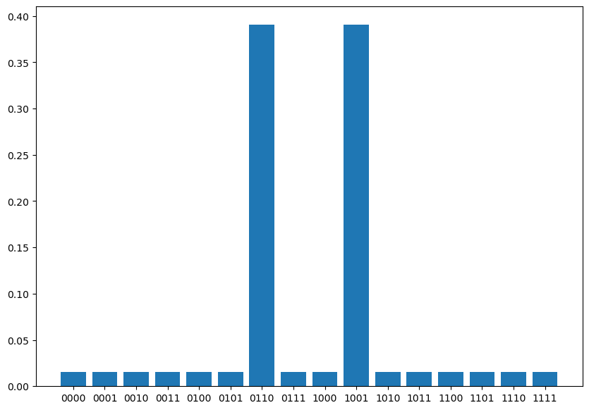
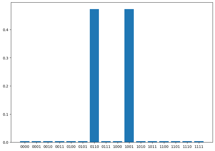
The probabilities of obtaining each state after the Grover algorithm with one or two repetitions can be observed in Fig.4.
III 2WQC Grover
The operation can be used in conjunction with the ancilla qubit and a modified oracle to obtain the desired states with probability equal to one, without any repetitions.
@C=1em @R=1.7em
& \lstick\ket0 \gateH \multigate2Oracle \meter
⋮⋮
\lstick\ket0 \gateH \ghostOracle \meter
\lstick\ket0 \qw \targ\qwx[-1]\qw \rstick\bra1
Our new Oracle doesn’t change phase of states but rather applies a gate to the ancilla qubit, which is controlled by the desired states.
In the context of solving the Sudoku circuit for 2WQC, Grover’s method is illustrated in Fig.6.
@C=1em @R=1em
& \lstick\ket0 \gateH \qw \ctrl1 \ctrl2 \qw \ctrl2 \ctrl1 \qw \meter
\lstick\ket0 \gateH \ctrl2 \targ \qw \ctrl1 \qw \targ \ctrl2 \meter
\lstick\ket0 \gateH \qw \qw \targ \ctrl1 \targ \qw \qw\meter
\lstick\ket0 \gateH \targ \qw \qw \ctrl1 \qw \qw \targ\meter
\lstick\ket0 \qw \qw \qw \qw \targ \qw \qw \qw \rstick\bra1
and the probabilities of the obtained states are shown in Fig.7.
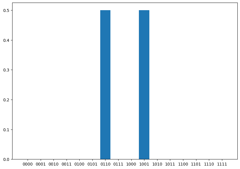
It is crucial to highlight that in the 2WQC Grover algorithm, the diffusion operator is not required since the correct states are automatically selected by the operation . Consequently, there is no requirement to repeat the oracle as in the case of the standard Grover’s algorithm.
IV Noise
This study presents an analysis of the influence of different quantum noise models on both the traditional Grover algorithm and the 2WQC version of the Grover algorithm. A single-qubit error channel is applied after each gate in the circuit. The types of error channels that will be discussed are as follows.
IV.1 Bit flip
This channel is modelled by the following Kraus matrices:
where is the probability of a bit flip (Pauli error).
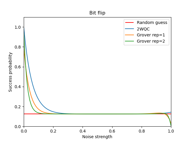
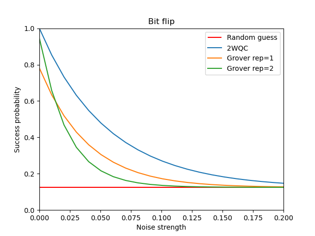
The results, Fig.8, indicate that 2WQC Grover is more resilient to this type of noise.
IV.2 Phase flip
This channel is modelled by the following Kraus matrices:
where is the probability of a phase flip (Pauli error).
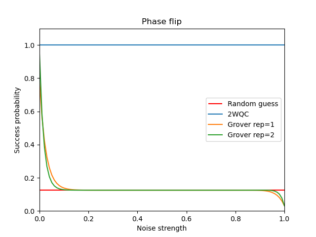
It is somewhat surprising that the 2WQC Grover is completely resilient to this type of noise, Fig.9.
IV.3 Phase damping
The interaction between the quantum system and its environment can result in the loss of quantum information without any changes in the qubit excitations. This phenomenon can be modelled by the phase damping channel, with the following Kraus matrices:
where is the phase damping probability.
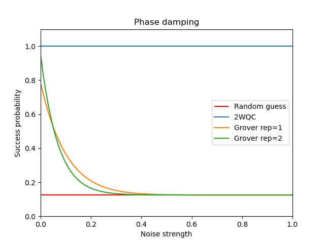
Once more, the 2WQC Grover is entirely resilient to this type of noise, Fig.10.
IV.4 Depolarizing channel
This channel is modelled by the following Kraus matrices:
where is the depolarization probability and is equally divided in the application of all Pauli operations.
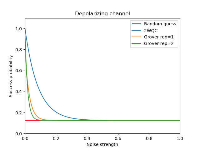
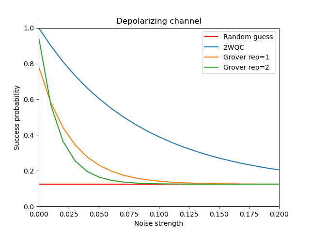
As in the case of bit flip noise, the 2WQC Grover is more resilient to this type of noise, Fig.11.
V Methods
VI Summary
The implementation of the 2WQC operation allows for the modification of the Grover algorithm, which now runs in a constant time complexity of , in contrast to the standard algorithm, which runs in a time complexity of . Moreover, it is more resilient to the various types of noise. In the case of phase flip and phase damping channels, the system is completely resilient. In the absence of noise, the 2WQC Grover algorithm is capable of identifying all states with absolute certainty, in contrast to the traditional Grover algorithm, which is only capable of identifying states with some (high) probability.
References
- Duda [2023] J. Duda, Two-way quantum computers adding cpt analog of state preparation, arXiv preprint arXiv:2308.13522 (2023).
- Grover [1996] L. K. Grover, A fast quantum mechanical algorithm for database search, in Proceedings of the twenty-eighth annual ACM symposium on Theory of computing (1996) pp. 212–219.
- Bergholm et al. [2018] V. Bergholm, J. Izaac, M. Schuld, C. Gogolin, S. Ahmed, V. Ajith, M. S. Alam, G. Alonso-Linaje, B. AkashNarayanan, A. Asadi, et al., Pennylane: Automatic differentiation of hybrid quantum-classical computations, arXiv preprint arXiv:1811.04968 (2018).
- Harris et al. [2020] C. R. Harris, K. J. Millman, S. J. van der Walt, R. Gommers, P. Virtanen, D. Cournapeau, E. Wieser, J. Taylor, S. Berg, N. J. Smith, R. Kern, M. Picus, S. Hoyer, M. H. van Kerkwijk, M. Brett, A. Haldane, J. F. del Río, M. Wiebe, P. Peterson, P. Gérard-Marchant, K. Sheppard, T. Reddy, W. Weckesser, H. Abbasi, C. Gohlke, and T. E. Oliphant, Array programming with NumPy, Nature 585, 357 (2020).
- Czelusta [2024] G. Czelusta, https://github.com/gczelusta/2wqc (2024), access: 12 czerwca 2024.