MSz: An Efficient Parallel Algorithm for Correcting Morse-Smale Segmentations in Error-Bounded Lossy Compressors

Abstract

This research explores a novel paradigm for preserving topological segmentations in existing error-bounded lossy compressors. Today’s lossy compressors rarely consider preserving topologies such as Morse-Smale complexes, and the discrepancies in topology between original and decompressed datasets could potentially result in erroneous interpretations or even incorrect scientific conclusions. In this paper, we focus on preserving Morse-Smale segmentations in 2D/3D piecewise linear scalar fields, targeting the precise reconstruction of minimum/maximum labels induced by the integral line of each vertex. The key is to derive a series of edits during compression time; the edits are applied to the decompressed data, leading to an accurate reconstruction of segmentations while keeping the error within the prescribed error bound. To this end, we developed a workflow to fix extrema and integral lines alternatively until convergence within finite iterations; we accelerate each workflow component with shared-memory/GPU parallelism to make the performance practical for coupling with compressors. We demonstrate use cases with fluid dynamics, ocean, and cosmology application datasets with a significant acceleration with an NVIDIA A100 GPU.

Introduction

The rapid advancement of high-performance computing (HPC) technologies has enabled the generation of vast quantities of scientific data, posing significant challenges to scientists regarding data storage, transmission, and visualization. As such, scientists recently started to explore compression, especially error-bounded lossy compression, to address the data challenges by ensuring efficient data management and utilization while limiting the amount of distortion introduced by compression.

The adoption of error-bounded lossy compression techniques, exemplified by algorithms like SZ [20, 22, 33, 37, 38], ZFP [23], and FPZIP [24], offers a pragmatic solution for reducing scientific data. These methodologies facilitate substantial data reduction while maintaining a predefined accuracy threshold, thus ensuring the utility of compressed datasets for immediate analysis and scientific exploration.

However, an emerging issue with lossy compressors is the inability to preserve topological features in decompressed data, even with bounded error. Topological inconsistencies between the original and decompressed data may result in misinterpretation of the data, even leading to erroneous scientific findings. Applications of these topological feature descriptors, such as Morse-Smale (MS) complexes and merge tress, proved the usefulness of science applications ranging from cosmology [32], material sciences [34], Earth sciences, to molecular dynamics [29, 5].

Even the tiniest variations, however small the compression error bound is, can induce significant alterations in the MS segmentation, thereby impacting scientists’ understanding of data. For example, a recent study showed that compressors often introduce alternations into topological features such as scalar field contour trees [35] and vector field critical points [21] in decompressed data, even with bounded pointwise error. As exemplified in Figure 1, we compress a molecular dynamics dataset using SZ3 and ZFP with relative error bounds ranging from $10^{-6}$ to $10^{-2}$, which all introduced discrepancies of topological segmentations induced by MS complexes up to 100%; the specific metric measures the discrepancies of segmentations by the percentage of points with a wrong segmentation ID, as explained later in this paper.

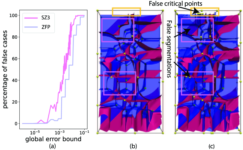
Figure 1: Impacts of lossy compression (SZ3 and ZFP) on MS segmentations of the Adenine Thymine (AT) dataset: (a) percentages of vertices with wrong segmentation labels w.r.t different error bound; (b) and (c): critical points and separatrices in the original data and SZ3’s decompressed data with a relative error bound of $10^{-3}$.

This research focuses on preserving Morse-Smale (MS) segmentations [28] in lossy compression workflows; such segmentations provide a preview of the Morse-Smale complex. MS segmentation consists of two significant components of the full MS complex: the extrema designated for each MS complex region and the delineations separating adjacent MS complex regions. Due to the high computational complexity of the MS complex, MS segmentations are used in diverse applications because they offer a cost-effective way to visualize topological segmentation for visualization and analyses.

To tackle inconsistencies of topological segmentations, we introduce a novel edit-based paradigm for preserving MS segmentations in error-bounded lossy decompressed data in 2D/3D piecewise linear scalar fields. Our method works directly on the decompressed data during the compression process, making it theoretically applicable to any error-bounded lossy compressor. Specifically, we identify a subset of data that requires edits, such that the MS segmentation of the decompressed data remains identical to that in the original dataset while also guaranteeing the global error bound. Since each MS segmentation region consists of a pair of extrema and the points included in the region, our method mainly focuses on preserving these two features by alternatively fixing extrema and integral lines until convergence within finite iterations of the loop: (1) computing the MS segmentation of the current data, (2) identifying the false data points (false critical or regular points), and (3) fixing the false data points until one can reconstruct the exact MS segmentation with the edits during decompression.

We address the performance and scalability of our method with shared-memory/GPU parallelism. While the efficient parallel computation of MS segmentation/complex is already a known challenge [28], the full realization of our vision requires careful parallelization design. Specifically, a key challenge is handling read-write and write-write conflicts when multiple threads attempt to modify the data concurrently. For example, if a vertex is adjacent to two critical points, during the iteration to fix multiple critical points, two parallel threads could simultaneously change the vertex’s value; we use atomic intrinsics to avoid such conflicts while maintaining high scalability. Later, this paper demonstrates a comprehensive performance analysis with CPUs and GPUs on a compute node of Lawrence Berkeley’s Perlmutter supercomputer. In summary, the contributions of this paper are multifold:

• A novel edit-based paradigm for preserving MS segmentation within error-bounded lossy decompressed data in 2D/3D piecewise linear scalar fields, theoretically applicable to any existing error-bounded lossy compressors;

• Efficient shared-memory/GPU parallelism that significantly accelerates individual components of our algorithm while addressing read-write/write-write conflicts;

  • As part of this contribution, a high-performance GPU algorithm for computing MS segmentation;

• Comprehensive evaluation of our method across various datasets, two off-the-shelf base compressors (SZ3 and ZFP), and parallel performance on both CPUs and GPUs.

1 Related Work

We review related work on error-bounded lossy compression, topology-preserving compression, and Morse-Smale complexes.

1.1 Error-Bounded Lossy Compression

Data compression techniques can be categorized into lossless and lossy compression based on whether information is lost during the compression process. Lossy compressors can attain higher compression ratios by discarding certain non-essential or redundant data while ensuring a specified level of data quality.

One can further categorize lossy compressors into non-error-bounded and error-bounded lossy compressors; we mainly focus on the latter category to preserve the MS segmentation of decompressed data. Error-bounded lossy compressors can achieve high compression ratios while guaranteeing data quality. However, few existing lossy compressors consider topology features in the decompressed data, which will impact disciplines that require post hoc analysis of the topological structure, thereby introducing deviations in the analytical results.

Error-bounded lossy compressors can be further divided into prediction-based or transformation-based lossy compressors. Examples of prediction-based compressors include the SZ series [20, 22, 33, 37, 38, 7, 6]. For example, SZ2 [33] uses the Lorenzo predictor combined with linear-scaling quantization to convert prediction residuals into integers, which are then encoded with customized Huffman coding or lossless compressors like ZSTD [2] and GZIP [1]. QoZ [27]is an optimization of SZ3, focusing on the quality of decompressed data. It is capable of automatically adjusting the compression based on user-specified quality objectives.

Transformation-based lossy compressors first transform data into an alternative representation, such as wavelet transformation and tensor decomposition, then compress data in the transformed domain. For example, ZFP [23] uses a custom orthogonal block transform to decorrelate data within blocks, transforming original data into sparsely distributed coefficients. These coefficients are then encoded for efficient compression, leveraging the reduced complexity of the transformed data to enhance compression efficiency. FPZIP [24] allows a specified number of bit planes to be ignored, making the data distortion controllable on demand. SPERR [18] is another transform-based lossy compressor that uses the CDF9/7 discrete wavelet transform and SPECK encoding algorithm. AE-SZ [26] and SRNN-SZ [25] are examples of another class of error-bounded lossy compressors that use neural networks.

1.2 Topology Preservation in Lossy Compression

Topology preservation is an emerging topic in the context of error-bounded lossy compression; to our knowledge, our work is the first attempt toward preserving Morse-Smale complexes by maintaining the consistency of topological segmentations.

Regarding scalar field topology, previous studies primarily focus on contour/merge tree preservation. Yan et al. [35] introduced TopoSZ to enhance the SZ 1.4 compression algorithm by integrating topological constraints informed by segmentations induced by contour trees. Soler et al. [31] developed a topology-controlled compression scheme to adaptively quantize data in individual topological features to preserve the persistence diagram subject to a persistence simplification threshold.

Regarding vector field topology, researchers have attempted to retain critical points, yet the preservation of separatrices and topological segmentations is done empirically. For example, Liang et al. [21, 19] presented a methodology for safeguarding critical points in piecewise linear and bilinear vector fields. Their method modifies the SZ compressor and incorporates a vertex-wise error bound for each grid point during compression to ensure the accurate preservation of critical points’ positions and types.

1.3 Morse-Smale Complexes and Segmentations

Table 1: Table of notations. Quantities in decompressed data are with hat, e.g., $\hat{f}_{i}$

Symbol	Meaning
$\xi$	Global error bound
$v_{i}$	The $i$th vertex
$L_{i}$	Vertex neighbors of $v_{i}$
$f_{i}$, $\hat{f}_{i}$	Scalar at $v_{i}$
$g_{i}$	Edited scalar at $v_{i}$
$\delta_{i}$	Edit at $v_{i}$
$m_{i}$, $\hat{m}_{i}$	Min label at $v_{i}$
$M_{i}$, $\hat{M}_{i}$	Max label at $v_{i}$

We summarize related work in MS complexes and segmentations and leave a detailed review of key definitions in the next section. MS complexes are a well-studied topological descriptor researched by the topological data analysis (TDA) and visualization communities. Constituents of MS complexes include critical points (maxima, minima, and saddles) and separatrices that connect saddles and extrema; the separatrices also partition the input manifold into regions with monotonous subregions, often referred to as MS segmentations.

In general, two flavors exist for MS complex computation: piecewise linear (PL) Morse theory [3, 9] and discrete Morse theory [11]. We refer readers to Lewiner et al. [17] for a comprehensive review and comparison between the two MS complex computation approaches. Our work primarily relies on the PL-based MS segmentation computation, and we formally review key assumptions and concepts of PL Morse theory in the next section.

With the PL Morse theory, one can further divide algorithms into boundary- and region-growing-based approaches. For boundary-based algorithms, Edelsbrunner et al. [9] first introduced the MS complex for piecewise linear 2-manifolds and 3-manifolds [8]. Gyulassy et al. [15] introduced the region-growing algorithm for analyzing Morse-Smale complexes, which is scalable for 3D or higher dimensions. Banchoff et al. [3] explored the critical points on piecewise linear 2-manifolds by analyzing the paths of steepest ascent and descent.

With Forman’s discrete Morse theory, Fugacci et al. [12] addressed the efficient computation of discrete Morse complexes on large, high-dimensional simplicial complexes. Gyulassy et al. [14] introduced a new algorithm for computing the Morse-Smale complex efficiently across different data scales and dimensions, which was later extended to a parallel computing framework [16].

As related to the parallel computation of MS complexes and segmentations, Beucher et al. [4] utilized watershed transformations to analyze and construct Morse-Smale complexes in the context of image processing and data analysis, which was optimized by Gabrielyan et al. [13] by leveraging GPU technology to the computational processes of the Morse-Smale complex. Yeghiazaryan et al. [36] combine path simplification with watershed transformations for efficiency.

2 Background: Morse-Smale Segmentation in Piecewise Linear Scalar Fields

This section reviews key concepts in piecewise linear MS segmentations (PLMSS), including critical points and integral lines. We refer readers to Maack et al. [28] for a comprehensive picture of PLMSS. Without loss of generality, 2D/3D PLMSS is represented by the label pair $\langle m_{i},M_{i}\rangle$ for each vertex $v_{i}$ in a triangular/tetrahedral mesh $\langle V,E\rangle$, where $V$ and $E$ is the set of vertices and edges. For ease of description, $L_{i}$ represents all vertex neighbors of $v_{i}$. Table 1 summarizes notations used in this paper.

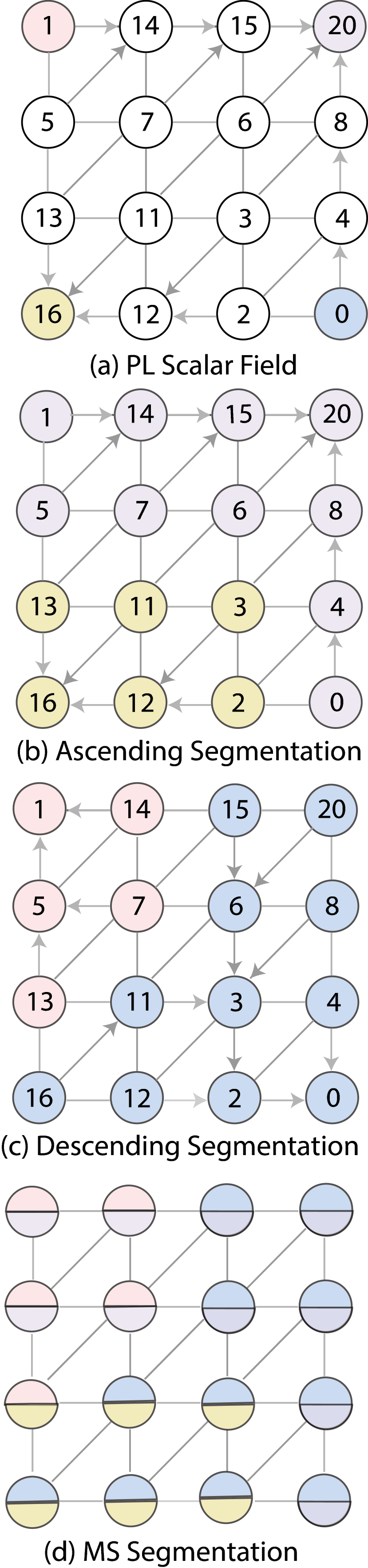
Figure 2: Constituents of MS segmentations.

MS complex generally partitions the data domain into segmentations with consistent gradient behavior; readers are referred to Edelsbrunner et al. [10] for a comprehensive background. Formally, A Morse function is a smooth map $f:\mathbb{X}\to\mathbb{R}$, where $\mathbb{X}$ is a compact manifold (in this research, $\mathbb{X}\subset\mathbb{R}^{2}$ or $\mathbb{R}^{3}$) without boundary, and all critical points of $f$ (locations where $\nabla f$ vanish) are nondegenerate and have distinct function values. At any regular point where $\nabla f\neq 0$, the integral line begins at the point and terminates at a critical point of $f$ in either forward or backward direction. An ascending/descending manifold of critical point $x\in\mathbb{X}$ consists of all regular points whose integral line terminates at $x$. The ascending and descending manifold form a Morse complex of $f$ and $-f$, respectively; the two Morse complexes’ intersection further form the Morse-Smale complex of $f$. Boundaries of ascending/descending manifold are also referred to as separatrices of the complex. For the practical computation of MS complexes, one can simulate the differentiability of piecewise linear functions. With the underlying triangulation of the piecewise linear domain $\mathbb{X}$, although the gradient field is discontinuous, this method simulates gradient flow behavior by approximating the gradient flow through the edges and faces of the triangulation. Analogs are defined for critical points, integral lines, and ascending/descending manifolds for constructing MS complexes, as further reviewed below.

Critical points in PL scalar field $f$ reside on the vertices of the underlying triangulation, and they are extracted and classified based on the lower/upper star of a vertex, as exemplified in Figure 2(a). The lower star of a vertex $v$, represented by $St_{-}(v)$, comprises all simplices within the triangulation where $v$ is the vertex with the maximum value according to the scalar field. One can determine if a vertex $v$ is critical and categorize critical points into the following types with $v$’s lower and upper stars. For example, $v$ is a minimum if $St_{-}(v)$ is empty, which implies that there are no simplices for which $v$ is the vertex with the highest scalar value (e.g., the two nodes with scalar values 0 and 1 in Figure 2(a)). This can be represented as $St_{-}(v)=\emptyset$; $v$ is a maximum if $St_{+}(v)$ is empty, indicating no simplices have $v$ as their lowest vertex $St_{+}(v)=\emptyset$ (e.g., 16 and 20 in Figure 2(a)).

Integral lines in PL scalar fields. In PL scalar fields, integral lines of gradient vector fields are constructed by monotonic paths consisting of edges in the triangulation. For example, in Figure 2(b), $5\rightarrow 14\rightarrow 15\rightarrow 20$ is an integral line that extends toward the highest/lowest adjacent vertices until a maximum/minimum is met. We further distinguish backward and forward integral lines based on the ascending/descending direction an integral line is tracing toward.

Ascending/descending segmentations in PLMSS. Once integral curves are traced, one can find the minimum/maximum that a vertex $v$ flows to and further define MS segmentation in PL scalar fields. Starting from $v$, we denote its converging critical points as the maximum label $M$ and minimum label $m$ following the ascending and descending integral lines. In the PL complex, two vertices $v_{1}$ and $v_{2}$ are in the same MS segmentation if their minimum/maximum labels $\langle m_{1},M_{1}\rangle$ and $\langle m_{2},M_{2}\rangle$ are identical. For example, in Figure 2, nodes in b and c, respectively, are colored by maximum and minimum labels; nodes in d are colored by both maximum and minimum labels simultaneously.

3 Problem Statement

We formulate the preservation of MS segmentations in 2D and 3D piecewise linear scalar fields. The inputs of our algorithm include both original data $f$ and decompressed data $\hat{f}$, assuming both data versions are available at the compression time. We assume all scalar field data are Morse; that is, for any two vertices $i$ and $j$, we have $f_{i}\neq f_{j}$. We use simulation of simplicity (SoS) [10] to handle such degeneracy for real-world data. The outputs of our algorithm are a series of edits $\{\delta_{i}\}$; with the edits, one can derive the final edited value at vertex $i$ as $g_{i}=\hat{f}_{i}+\delta_{i}$. The edited value shall satisfy the following constraints:

Preservation of the global error bound. We must guarantee that the final augmented value is subject to the user-prescribed absolute error bound $\xi$, that is, $\left|f_{i}-g_{i}\right|\leq\xi$.

Preservation of MS segmentations. Let $M$ and $m$, respectively, denote the maximum and minimum labels in MS segmentations of the original data, and let $\hat{M}$ and $\hat{m}$ denote the counterparts in the decompressed data. This research aims to precisely align $\hat{M}$ with $M$ and $\hat{m}$ with $m$. That is, for any vertex $v_{i}$, we have $M_{i}=\hat{M}_{i}$ and $m_{i}=\hat{m}_{i}$.

Preservation of maxima/minima. Our definition of MS segmentation preservation also implies that all extrema are preserved without any false positives or negatives. Under the premise that the location and type of critical points in the decompressed data are identical to those in the original data, to ensure that $\hat{M}$ is precisely equal to $M$, it is necessary to align the label of each regular point $i$ in the decompressed data with its corresponding label in the original data. We guarantee the preservation of extrema without any false positives or false negatives, which are formally defined in the next section.

4 Methodology

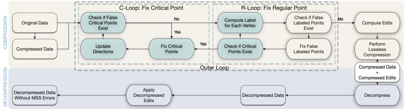
Figure 3: Workflow of our method. Our method mainly happens during the compression process. The blocks with a blue background color are the processes in which we used parallel acceleration. There are two distinct inner loops: (1) the C-loop iteratively fixes all the false critical points in the decompressed data until no false critical points exist; (2) the R-loop fixes all the false labeled regular points. The outer loop iteratively executes the critical point loop and regular point loop until there is no false critical point and false labeled point. Upon completion of the outer loop, the edits are losslessly compressed and used as the final output along with the compressed data. In the decompression process, the decompressed edits would be applied to the decompressed data, obtaining the data without MSS errors.

This section describes the theoretical workflow of computing edits for preserving MS segmentations, as illustrated in Figure 3. The derivation of edits is an iterative process involving two distinct loops: the critical point loop (C-loop, Section 4.1) and the regular point loop (R-loop, Section 4.2). The rationale for alternating the two loops is that (1) the correctness of critical points is necessary for fixing regular points, and (2) fixing regular points may introduce new false critical points to be fixed further. We discuss the convergence throughout this section and leave all parallel computation aspects in the next section.

Figure 4: Illustration of our methodology, thick circles represent the maximum, the color of each circle represents the maximum label of the vertex, arrows represent the ascending direction of each vertex: Ascending segmentation of (a) the original data; (b) the decompressed data with the node with value 27 as a false positive maximum; (c) the modified decompressed data with node five as the falsely labeled regular point; (d) the modified decompressed data with the node with value 21 as the false positive maximum; (e) the fixed decompressed data without a false critical point or regular point.

4.1 Critical Point Loop (C-Loop)

We fix four types of false critical points:false positive maxima (FPmax), false positive minima (FPmin), false negative maxima (FNmax), and false negative minima (FNmin). A sublevel loop handles each false type; for example, the FPmax loop executes multiple times until no FPmax exists, followed by the FPmin loop. The entire C-loop sequentially executes the four subloops in each iteration and exits when no false critical point remains.

Readers may skip the mathematical reasoning below, but the key to (sub)loop convergence is incurring changes that only decrease (or keep) scalar values at each iteration. That is, denoting $g_{i}^{(k)}$ as the edited value at vertex $i$ during the $k$th iteration ($k\in\mathbb{I}$), we have

$$\hat{f}_{i}=g_{i}^{(0)}\geq\cdots\geq g_{i}^{(k)}\geq g_{i}^{(k+1)}\geq\cdots>f_{i}-\xi,$$ (1)

and $g_{i}^{(k)}$ progressively approaches to the lower bound $f_{i}-\xi$. As such, one can make the relationship between scalars on neighboring vertices consistent with that of the original data; formally, for arbitrary two vertices $i$ and $j$, we have

Lemma 1.

One can find a finite number $k$ of iterations such that $g_{i}^{(k)}<g_{j}^{(k)}$, if initially $g_{i}^{(0)}>g_{j}^{(0)}$ and $f_{i}<f_{j}$.

Backed by Lemma 1, we design decreasing edits to fix four false cases. Each decreasing edit applies to the vertex with a false critical point (FPmax or FNmin) or a neighbor vertex of the false critical point (FPmin or FNmax), as exemplified below.

4.1.1 False Positive Maximum

Definition 1 (FPmax).

A maximum $g_{i}$ is false positive if $g_{i}>g_{j}$ for all vertex neighbors $j\in L_{i}$, but one can find at least one neighbor $j$ such that $f_{i}<f_{j}$.

We construct a sequence of iterations for all vertices, following Equation (1), to iteratively eliminate all FPmax:

$$g_{i}^{(k+1)}:=\left\{\begin{array}[]{ll}\nicefrac{{\left(g_{i}^{(k)}+f_{i}-\xi\right)}}{{2}},&\mbox{\leavevmode\nobreak\ if $g_{i}^{(k)}$ is FPmax}\\ g_{i}^{(k)},&\mbox{\leavevmode\nobreak\ otherwise.}\end{array}\right.$$ (2)

Note that $g_{i}^{(k)}$ monotonically decreases toward the lower bound $f_{i}-\xi$ as $k$ increases. We speculate three possible outcomes at an arbitrary iteration $k$:

• Case I: $g_{i}^{(k)}$ remains an FPmax, requiring at least another iteration;

• Case II: $g_{i}^{(k)}$ becomes non-maximum without introducing any new FPmax; for the moment, $g_{i}^{(k)}$ is fixed;

• Case III: $g_{i}^{(k)}$ becomes non-maximum but introduces at least one new FPmax $g_{j}^{(k+1)}$ at a neighboring vertex $j$;

Cases I and II are trivial. In Case III, the newly introduced FPmax at $j$ will be eventually fixed in later iterations without making $i$ an FPmax again. Specifically, per Definition 1, one can find a vertex $j^{\prime}\in L_{j}$ that is ascending in the original data ($f_{j}<f_{j^{\prime}}$); no matter if $j^{\prime}$ is $i$ or not, with additional iterations with whichever cases, per Lemma 1, neither $i$ nor $j$ will become FPmax with an additional finite number of iterations.

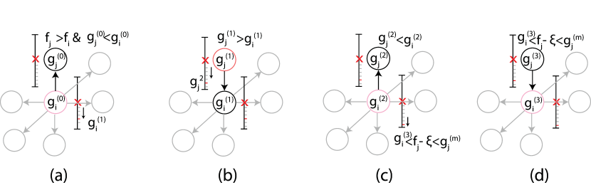
Figure 5: Example of the process of fixing a false positive maximum $v_{i}$ (the vertex in the center). The vertex with a colored border represents a false positive maximum at each iteration, the line beside the vertex represents the value range of the vertex, and the red x represents its scalar value in the original data, arrows represent the relationship between the magnitude of the scalar values between vertices. At each iteration, we reduce the values of $v_{i}$ or $v_{j}$ until $g_{i}^{(k)}<f_{j}-\xi<g_{j}^{(k)}$, then $v_{i}$ would not become a new false positive maximum again.

We use Figure 5 to help understand Case III further. Assume that $v_{i}$ is a false positive maximum and $v_{j}\in L_{i}$, satisfying $f_{j}>f_{i}$ while $g_{j}^{(0)}<g_{i}^{(0)}$. During the first iteration, we decrease $g_{i}^{(0)}$ to $g_{i}^{1}$ that $g_{i}^{(1)}<g_{j}^{(1)}$, making $v_{i}$ become a regular point and $v_{j}$ a new false positive maximum in this example. In line with our strategy, we decrease $g_{j}^{(1)}$ in the subsequent iteration, potentially reinstating $i$ as a new false positive maximum again. This iterative process might repeat; note that $f_{i}-\xi<f_{i}<f_{j}<f_{j}-\xi$, and our approach incrementally drives $i$ and $j$ closer to their lower bounds. Therefore, within a finite number of iterations, $g_{i}$ and $g_{j}$ will intersect, resulting in $g_{i}<f_{j}-\xi<g_{j}$ in subsequent iterations, at which point $v_{i}$ will no longer become a new false positive maximum.

4.1.2 False Positive Minimum

Definition 2 (FPmin).

A minimum $g_{i}$ is false positive if $g_{i}<g_{j}$ for all $j\in L_{i}$ but one can find at least one $j$ such that $f_{i}>f_{j}$.

Unlike fixing FPmax, assuming $g_{i}^{(k)}$ is FPmin, we decrease the value at the ascending neighbor $j$, such that $g_{j}^{(k)}(j\in L_{i})$ is the maximal among the neighbors of $i$, and we have

$$g_{j}^{(k+1)}:=\left\{\begin{array}[]{ll}\nicefrac{{\left(g_{j}^{(k)}+f_{j}-\xi\right)}}{{2}},&\mbox{\leavevmode\nobreak\ if $g_{j}^{(k)}$ is maximal among $j\in L_{i}$}\\ g_{j}^{(k)},&\mbox{\leavevmode\nobreak\ otherwise.}\end{array}\right.$$ (3)

While one could alternatively fix the FPmin by increasing the value on the same vertex, we impose decreasing edits across all types of false critical points to guarantee convergence across the iterative workflow; otherwise, incompatible strategies may not lead to convergence. We omit the detailed analysis of three possible cases (remaining as an FPmin or becoming a non-minimum with or without introducing a new FPmin), but the convergence of the FPmin iterations can be achieved in a similar way as in Section 4.1.1.

4.1.3 False Negative Maximum/Minimum

Definition 3 (FNmax/FNmin).

A non-maximum (or non-minimum) $g_{i}$ is false negative if $f_{i}>f_{j}$ (or $f_{i}<f_{j}$) for all $j\in L_{i}$.

Specifically, for an FNmax $g_{i}$, we reduce its ascending neighbor’s value and have

$$g_{j}^{(k+1)}:=\left\{\begin{array}[]{ll}\nicefrac{{\left(g_{j}^{(k)}+f_{j}-\xi\right)}}{{2}},&\mbox{\leavevmode\nobreak\ if $g_{j}^{(k)}$ is maximal among $j\in L_{i}$}\\ g_{j}^{(k)},&\mbox{\leavevmode\nobreak\ otherwise.}\end{array}\right.$$ (4)

For an FNmin $g_{i}$, we decreasing its own scalar value:

$$g_{i}^{(k+1)}:=\left\{\begin{array}[]{ll}\nicefrac{{\left(g_{i}^{(k)}+f_{i}-\xi\right)}}{{2}},&\mbox{\leavevmode\nobreak\ if $g_{i}^{(k)}$ is FNmin}\\ g_{i}^{(k)},&\mbox{\leavevmode\nobreak\ otherwise.}\end{array}\right.$$ (5)

Note that both strategies comply with Equation (1) so that the iterations are provably convergent with finite iterations.

4.2 Regular Point Loop (R-Loop)

Once all false critical points are fixed, the next step is to fix all regular points’ maximum and minimum labels in the decompressed data. For a falsely labeled regular point, our method involves three steps in each iteration: (1) compute the ascending/descending integral lines in the original data and the edited data $g^{(k)}$ in the current iteration, (2) locate the “trouble maker” as the first occurrence of discrepancy along the integral lines, (3) fix the troublemaker by a local edit. Similar to the strategies in C-loops, the local edit, which has to decrease the decompressed value, is applied to the troublemaker or the troublemaker’s ascending/descending neighbor. Once the R-loop is finished, we return to the C-loop to address any new false positive critical points introduced by the R-loop.

For a false descending labeled regular point, let $v_{t}$ represent $v_{i}$’s descending neighbor in the original data, we decrease the value of $v_{t}$:

$$g_{v_{t}}^{(k+1)}:=\nicefrac{{\left(g_{v_{t}}^{(k)}+f_{v_{t}}-\xi\right)}}{{2}}.$$ (6)

For a false ascending labeled regular point, let $v_{t}$ represents $v_{i}$’s ascending neighbor in the decompressed data, we use the same equation to update $v_{t}$.

Figure 4(c) demonstrates the example of a false labeled point. In the original data, the maximal neighbor of node with value 5 should be towards the node with value 23, which changes to the node with value 24 in the decompressed data. By modifying the relationship between the values of the node with value 23 and the node with value 24, we can realign the integral line back to its correct direction.

Because C- and R-loops only introduce decreasing edits to the data for the entire outer loop, one can fix all critical and regular points within a finite number of iterations. Later we demonstrate how the number of iterations of inner and outer loops vary with different datasets and (parallel) execution orderings.

5 Parallel Computation and Compression of Edits

This section describes the shared-memory/GPU parallelism that significantly accelerates individual components of our algorithm.

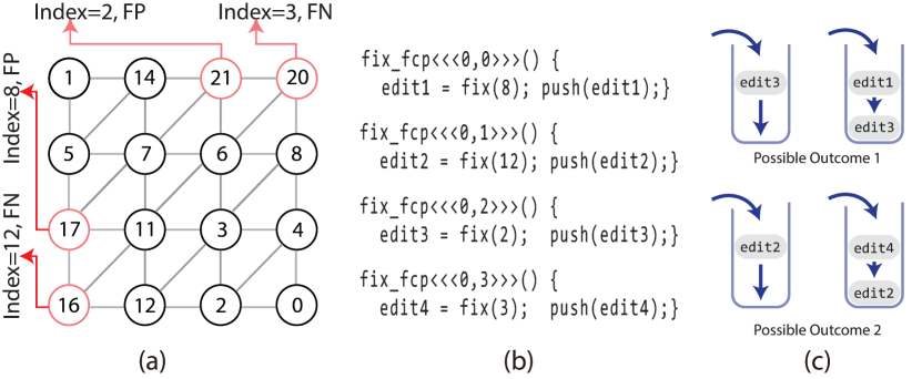
Figure 6: Fixing false critical points with multiple threads: (a) the PL scalar field, red circles representing false critical points, (b) each thread assigned with a false critical point, and (c) each edit is pushed into a lock-free stack.

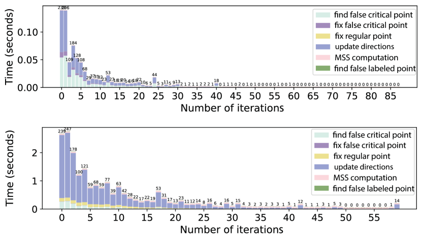
Figure 7: Timings of each task across outer loop iterations, with numbers above each bar chart denoting the count of sub-iterations per iteration. The top and bottom, respectively, is timings with GPU acceleration and CPU parallelism with 32 threads.

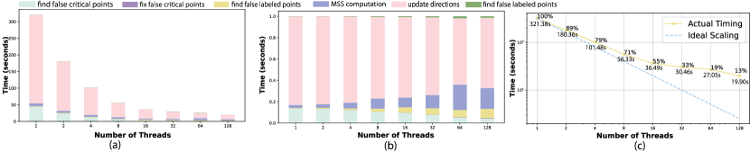
Figure 8: Strong scalability study for the viscous fingering dataset with OpenMP: (a) performance breakdown and (b) percentage breakdown of computational tasks w.r.t the number of threads; (c) strong scalability study on the end-to-end time.

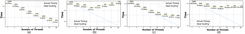
Figure 9: Strong scalability study of the four tasks w.r.t the number of threads used in our experiment (blue line: actual timing, red line: ideal scaling), percentages at data points represent the observed efficiency, and numbers show the actual timing. (a) find the false critical points; (b) fix false critical points; (c) update directions; (d) MSS computation.

Table 2: Timings of various tasks of our method on the Nyx dataset.

	Serial	OpenMP (Optimal)	CUDA	GPU Accel. cf. OpenMP	GPU Accel. cf. Serial
End-to-end	1192.38s	110s	17s	6$\times$	198$\times$
Find false critical points	1.202s	0.26s	0.008s	32$\times$	150$\times$
Update directions	10.46s	0.6s	0.014s	42$\times$	700$\times$
Fix false critical points	0.009s	0.002s	0.00038s	5$\times$	23$\times$
MSS computation	17.87s	2.7s	0.051s	52$\times$	350$\times$

5.1 Parallel C-Loop

All subroutines that are necessary for the C-loop are parallelized, including (1) finding false critical points, (2) fixing false critical points, and (3) updating directions for each vertex, as highlighted in Figure 3.

Find false critical points (Parallel-over-vertices). This process is highly amenable to parallelization because it only requires local comparisons for each point to ascertain whether it is a critical point. We set each thread to process an individual data point; if identified as a critical point, compare it with its corresponding type in the original dataset. We maintain a buffer with the length of the data to record the false critical points. This procedure creates an occasion where multiple threads concurrently access and manipulate the same buffer, leading to a write-write conflict. To address these conflicts, we used atomic operations (atomic_add_fetch() on CPUs and atomicAdd() on NVIDIA GPUs) to ensure data integrity and avoid the potential overwriting issues in the stack.

Fix false critical points (Parallel-over-critcal-points). Upon completing the process of getting false critical points, each thread is responsible for fixing a false critical point. If multiple threads concurrently attempt to modify the same data point, as shown in Figure 6, leading to a write-write conflict, then only one modification will be retained, which is preemptive. This preemptive approach introduces randomness into the fix process, meaning each iteration’s fixed false critical points are random. However, given that our approach iteratively checks for false critical points and performs modifications, any uncorrected false critical points are deferred to the subsequent iteration. Ultimately, this ensures that all false critical points are addressed and rectified.

Update direction (Parallel-over-vertices). We must update the ascending/descending direction in every iteration (including those in the R-loop) that changes the decompressed data. Computing the direction for each vertex involves a local comparison of scalar values between each point and its neighbors, well-suited for parallel computation. Here, we simply assign each vertex to a thread to update its ascending/descending direction.

5.2 Parallel R-Loop

The only component we currently parallelize in the R-loop is the computation of MS segmentation, recognizing that this process is inherently the most computationally expensive and dominates the execution time. All other subroutines, including finding troublemakers and fixing falsely labeled points, are currently in serial.

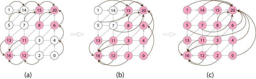
Figure 10: Parallel computation of maximum labels with path compression: pink nodes representing vertices that are already assigned to a maximum, gray arrows representing the direction of its largest neighbor, and black curves representing the current vertex assignment.

MSS computation (Parallel-over-vertices) We adopted the concept of path compression [30], as used by Maack et al. [28], for the computation of Morse-Smale segmentation. Taking ascending segmentation as an example (as shown in Figure 10), in brief, path compression involves utilizing a (lock-free) list to track regular points that have not yet found their maximum. For these points, the method seeks their largest neighbor, updating each point’s value in the list to that of its largest neighbor’s largest neighbor. If the value of a point $v$ remains unchanged after the update, meaning the largest neighbor’s largest neighbor is itself, it indicates that $v$ has been assigned to a maximum. The iteration concludes once every point has successfully determined its maximum.

5.3 Lossless Compression of Edits

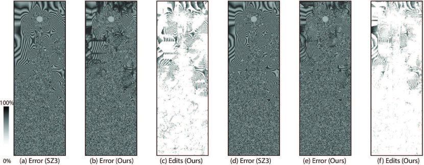
Figure 11: Spatial distribution of error and edits with error bounds of $7\times 10^{-4}$ (a, b, and c) and $10^{-3}$ (d, e, and f) based on SZ3.

Once all iterations converge and exit with no false critical/regular points, the last step is to store the edits compactly as metadata appended to the lossy compressor’s outputs. Each edit $\delta_{i}$ is represented with a key-value pair, the key being the vertex index and the value being the floating-point representation of the edits. We compress the indices and edit values separately. Regarding the indices, we first sort them in ascending order and compress the differential sequence. For example, ordered integers $\{1,35,36,421,422,423,\ldots\}$ will be represented by $\{1,34,1,385,1,1,\ldots\}$. The rationale is based on the observation that our edits are sparsely distributed (Figure 11) yet have continuous patches in the domain. As such, storing the differentials makes it possible to maximize the use of run-length encoding (RLE) and Huffman coding before offloading the data to a lossless compressor such as ZSTD [2] or GZIP [1].

6 Evaluation of Edited Data

Dataset	Dimensions
Red Sea	$500\times 500\times 50$
Adenine Thymine	$177\times 95\times 48$
Fingering	$128^{3}$
Nyx	$512^{3}$
Earthquake	$750\times 375\times 100$
Heated Flow	$150\times 450$
CESM-ATM	$1800\times 3600$

Table 3: Datasets used in our experiments.

We evaluate our method with seven datasets in Table 3 and evaluate the resulting accuracy in MS segmentation based on two state-of-the-art error-bounded lossy compressors, SZ3 and ZFP. Evaluation metrics are enumerated below.

MSS distrotion is a metric for quantifying the distortion degree of the MSS, calculated by the ratio of the number of false cases to the total number of data points. PSNR distrotion curves a standard tool to compare compression quality with varying bit rates. Overall Compression Ratio (OCR) is the compression ratio after the combination of edits, calculated by the combined size of compressed edits and data over the original data’s size. Edit ratio is the proportion of data points requiring modification in the decompressed data. Overall bit rate (OBR) is the bit rate (average bits per compressed data point) with the combination of compressed data and edits. Right labeled ratio is the percentage of points in the data with correct MSS labels, calculated by the number of right labeled points over the number of points in the data.

6.1 Fixed-Error-Bound Comparison

We demonstrate that our method can fix MS segmentation from arbitrary outputs from different compressors and error bounds, as shown in Figure 12. We can observe that the size of the edits required is roughly proportional to the magnitude of the global error bound. This is reasonable because as the global error bound increases, implying that more errors are introduced into the data, the error rate in the MSS escalates, thereby necessitating a greater number of edits. For more complex datasets, such as CSEM, Nyx, and viscous fingering, the edit ratio required for MSS restoration is noticeably higher than other datasets. Another observation is that edits required by ZFP are generally lower than those for SZ3, while OCR is higher overall than ZFP because ZFP’s original compression ratio is lower than SZ3.

6.2 Fixed-Bit-Rate Comparison

We evaluate our method across various datasets to identify the optimal overall bit rate (after the combination of edits) achievable on SZ3 and ZFP. We run an ensemble of experiments with various error bounds and find relatively the same (overall) bit rate with both SZ3 and ZFP to evaluate the preservation of MSS. With comparable bitrates, the original decompressed data from SZ3/ZFP exhibit varying degrees of MSS distortion across different datasets. Despite a certain bitrate increase due to the introduction of additional edits, as illustrated in the MSS/PSNR distortion plots, our method still ensures the precise preservation of the MSS. From the MSS/PSNR distortion, we can observe that there is a certain balance between OBR and the preservation of MSS. When the original bitrate is low, it implies a greater deviation between the decompressed data and the original data, leading to a higher error rate in the MSS, which, in turn, requires more edits. Conversely, when the original bitrate is high, the deviation between the decompressed and original data is reduced, lowering the error rate in the MSS and decreasing the necessary edits.

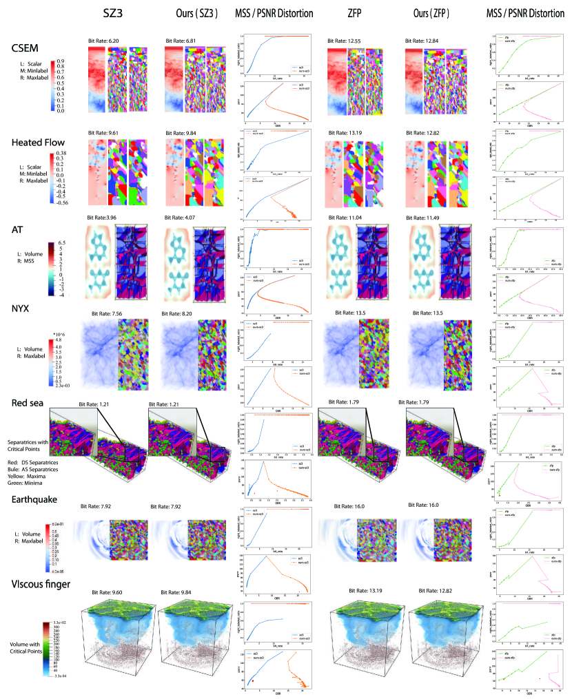
Figure 12: Fixed-error-bound comparison of lossy compressors on different datasets.

Figure 13: Fixed-bit-rate comparison of lossy compressors on fixed bit rate on different datasets.

7 Performance Evaluation

We evaluate the scalability and performance of our algorithm with both shared-memory CPU and GPU implementations. We use two datasets, Nyx ($512^{3}$) and viscous fingering ($128^{3}$), for performance studies because of their larger size and higher topological complexity than others. We use one CPU node (2$\times$ AMD EPYC 7763 with 512 GB of DDR4 memory) and one GPU node (single AMD EPYC 7763 CPU with 256 GB of DDR4 DRAM and four NVIDIA A100 GPUs) on the Perlmutter supercomputer at National Energy Research Scientific Computing (NERSC). Our implementation is based on C++, OpenMP, and CUDA; only a single GPU is used for benchmarking.

We measure performance with the end-to-end running time and four mini-benchmarks that evaluate the parallelization of (1) finding false critical points, (2) fixing critical points, (3) updating directions, and (4) MSS computation. For the mini-benchmarks, we artificially reset the data to the initial status the first time the subroutine is called. To ensure robustness and accuracy in our results, each mini-benchmark was executed 1,000 times, and the mean running time was recorded.

CPU strong scaling. Figure 8 shows the decreasing end-to-end running time with increasing CPU threads. We also demonstrated the timing breakdown for individual subroutines; for example, updating directions takes up to 80% of the time because all vertices’ directions must be updated whenever there is a change in the data. Figure 9 demonstrates the timings of the four mini-benchmarks with different numbers of threads. Finding critical points and updating directions are highly efficient because both are computationally simplistic. Fixing critical points is not as efficient as other subroutines because the number of false critical points is relatively fewer than the number of vertices, which may lead to under-utilization of hardware resources. Timings of the MSS computation flatten after eight threads but still decrease slowly with more threads; the early termination of integral lines with path compression causes imbalanced workloads.

GPU acceleration. Table 2 shows GPU acceleration of the end-to-end and mini-benchmarks. We achieved a $6\times$ acceleration in the end-to-end performance compared with using all 128 threads on the CPU node; the acceleration is $198\times$ compared with the serial execution. We did not reach an even higher ratio primarily because there are a few serial subroutines (e.g., finding the troublemaker and fixing falsely labeled points) and frequent GPU-CPU data exchange due to the serial subroutines on the CPU. For the mini-benchmarks, compared with serial execution with one single CPU, our GPU implementation achieves up to $700\times$ speed up across all tasks; it is worth mentioning that the MSS computation reached a $350\times$ and $52\times$ speedup, respectively, compared with serial and the best OpenMP performance.

Figure 7 presents an additional performance visualization across multiple C- and R-loops, comparing performance on a CPU (with 32 threads) and a GPU. Across both settings, a notable decrease in time and the number of sub-iterations is observed with increasing iteration. This is because the number of false critical/regular points decreases as the iteration progresses. Notably, the two settings are inconsistent in the total number of iterations and the number of sub-iterations within each iteration. This is because of the parallelism we applied to fix false critical points, as discussed in Section 5.1, which introduces randomness into the results. In each iteration, updating directions for each vertex accounts for a significant portion of the time, approximately 80% for CPU and 50% for GPU. This is followed by the process to find false critical points, around 10% for CPU and 40% for GPU.

8 Limitations

Our method aims at the precise preservation of Morse-Smale segmentations in 2D/3D piecewise linear scalar fields. However, there remains considerable scope for further enhancements in our approach. Firstly, while our method can ensure the precise preservation of the MSS, but not the MSC, it might fall short of accurately reconstructing saddle points and saddle-saddle connections. Secondly, our approach currently uses a straightforward lossless compression for edits, which presents significant room for improvement, potentially elevating the overall compression ratio. Our method’s objective is to preserve 100% of MSS; however, not all MSS components are equally significant. Determining how to retain essential MSS features while disregarding the less critical ones is another area where our method could be refined. Lastly, numerous aspects of our parallel section can be further optimized, such as reducing the time for data transfer and exploring strategies to mitigate the randomness in the critical point loop induced by the preemptive mechanism.

9 Conclusions and Future Work

We introduced a novel method for preserving MS segmentation within error-bounded lossy decompressed data in 2D/3D piecewise linear scalar fields. The core strategy involves generating a sequence of edits at the time of compression; these edits are then applied to the decompressed data, ensuring precise MSS reconstruction while guaranteeing the global error bound. Our approach also incorporates an efficient shared-memory/GPU parallelism that substantially enhances the speed of each component of our algorithm while carefully managing read-write and write-write conflicts. This introduces a high-performance GPU algorithm dedicated to computing MS segmentation. We evaluated our methods with several datasets from fluid dynamics, ocean, and cosmology application datasets. Also, we evaluated the capability to preserve MSS among state-of-the-art error-bounded lossy compressors.

We plan to improve our method in various aspects. First, the compression of edits is straightforwardly achieved through lossless compression, yet this aspect offers substantial room for improvement, potentially enhancing the final compression ratio. Second, our method can be extended to preserve the Morse-Smale complex by incorporating the preservation of saddles and saddle-saddle connectors into our current approach.

- [1] GZIP. https://www.gzip.org/.
- [2] ZSTD. http://www.zstd.net.
- [3] T. F. Banchoff. Critical points and curvature for embedded polyhedral surfaces. The American Mathematical Monthly, 77(5):475–485, 1970.
- [4] S. Beucher and C. Lantuéjoul. Use of watersheds in contour detection. vol. 132, 01 1979.
- [5] H. Bhatia, A. G. Gyulassy, V. Lordi, J. E. Pask, V. Pascucci, and P.-T. Bremer. Topoms: Comprehensive topological exploration for molecular and condensed-matter systems. Journal of Computational Chemistry, 39(16):936–952, 2018. doi: 10 . 1002/jcc . 25181
- [6] S. Di and F. Cappello. Fast error-bounded lossy hpc data compression with sz. In 2016 IEEE International Parallel and Distributed Processing Symposium (IPDPS), pp. 730–739, 2016. doi: 10 . 1109/IPDPS . 2016 . 11
- [7] S. Di and F. Cappello. Optimization of error-bounded lossy compression for hard-to-compress hpc data. IEEE Transactions on Parallel and Distributed Systems, 29(1):129–143, 2018. doi: 10 . 1109/TPDS . 2017 . 2749300
- [8] H. Edelsbrunner, J. Harer, V. Natarajan, and V. Pascucci. Morse-smale complexes for piecewise linear 3-manifolds. In Proceedings of the Nineteenth Annual Symposium on Computational Geometry, SCG ’03, p. 361–370. Association for Computing Machinery, New York, NY, USA, 2003. doi: 10 . 1145/777792 . 777846
- [9] H. Edelsbrunner, J. Harer, and A. Zomorodian. Hierarchical morse—smale complexes for piecewise linear 2-manifolds. Discrete & Computational Geometry, 30:87–107, 2003.
- [10] H. Edelsbrunner and E. P. Mücke. Simulation of simplicity: A technique to cope with degenerate cases in geometric algorithms. ACM Transactions on Graphics, 9(1):66–104, 1990.
- [11] R. Forman. Morse theory for cell complexes. Advances in Mathematics, 134(1):90–145, 1998. doi: 10 . 1006/aima . 1997 . 1650
- [12] U. Fugacci, F. Iuricich, and L. D. Floriani. Computing discrete morse complexes from simplicial complexes, 2018.
- [13] Y. Gabrielyan, V. Yeghiazaryan, and I. Voiculescu. Parallel partitioning: Path reducing and union–find based watershed for the gpu. In 2022 IEEE International Conference on Image Processing (ICIP), pp. 1501–1505, 2022. doi: 10 . 1109/ICIP46576 . 2022 . 9897372
- [14] A. Gyulassy, P.-T. Bremer, B. Hamann, and V. Pascucci. A practical approach to morse-smale complex computation: Scalability and generality. IEEE Transactions on Visualization and Computer Graphics, 14(6):1619–1626, 2008. doi: 10 . 1109/TVCG . 2008 . 110
- [15] A. Gyulassy, V. Natarajan, V. Pascucci, and B. Hamann. Efficient computation of morse-smale complexes for three-dimensional scalar functions. IEEE Transactions on Visualization and Computer Graphics, 13(6):1440–1447, 2007. doi: 10 . 1109/TVCG . 2007 . 70552
- [16] A. Gyulassy, V. Pascucci, T. Peterka, and R. Ross. The parallel computation of morse-smale complexes. In 2012 IEEE 26th International Parallel and Distributed Processing Symposium, pp. 484–495, 2012. doi: 10 . 1109/IPDPS . 2012 . 52
- [17] T. Lewiner. Critical sets in discrete morse theories: Relating forman and piecewise-linear approaches. Computer Aided Geometric Design, 30(6):609–621, 2013. Foundations of Topological Analysis. doi: 10 . 1016/j . cagd . 2012 . 03 . 012
- [18] S. Li, P. Lindstrom, and J. Clyne. Lossy scientific data compression with sperr. In 2023 IEEE International Parallel and Distributed Processing Symposium (IPDPS), pp. 1007–1017, 2023. doi: 10 . 1109/IPDPS54959 . 2023 . 00104
- [19] X. Liang, S. Di, F. Cappello, M. Raj, C. Liu, K. Ono, Z. Chen, T. Peterka, and H. Guo. Toward feature-preserving vector field compression. IEEE Trans. Vis. Comput. Graph., 29(12):5434–5450, 2023. doi: 10 . 1109/TVCG . 2022 . 3214821
- [20] X. Liang, S. Di, D. Tao, S. Li, S. Li, H. Guo, Z. Chen, and F. Cappello. Error-controlled lossy compression optimized for high compression ratios of scientific datasets. In 2018 IEEE International Conference on Big Data (Big Data), pp. 438–447, 2018. doi: 10 . 1109/BigData . 2018 . 8622520
- [21] X. Liang, H. Guo, S. Di, F. Cappello, M. Raj, C. Liu, K. Ono, Z. Chen, and T. Peterka. Toward feature-preserving 2d and 3d vector field compression. In 2020 IEEE Pacific Visualization Symposium (PacificVis), pp. 81–90, 2020. doi: 10 . 1109/PacificVis48177 . 2020 . 6431
- [22] X. Liang, K. Zhao, S. Di, S. Li, R. Underwood, A. M. Gok, J. Tian, J. Deng, J. C. Calhoun, D. Tao, Z. Chen, and F. Cappello. Sz3: A modular framework for composing prediction-based error-bounded lossy compressors, 2021.
- [23] P. Lindstrom. Fixed-rate compressed floating-point arrays. IEEE Transactions on Visualization and Computer Graphics, 20(12):2674–2683, 2014. doi: 10 . 1109/TVCG . 2014 . 2346458
- [24] P. Lindstrom and M. Isenburg. Fast and efficient compression of floating-point data. IEEE Transactions on Visualization and Computer Graphics, 12(5):1245–1250, 2006. doi: 10 . 1109/TVCG . 2006 . 143
- [25] J. Liu, S. Di, S. Jin, K. Zhao, X. Liang, Z. Chen, and F. Cappello. Srn-sz: Deep leaning-based scientific error-bounded lossy compression with super-resolution neural networks, 2023.
- [26] J. Liu, S. Di, K. Zhao, S. Jin, D. Tao, X. Liang, Z. Chen, and F. Cappello. Exploring autoencoder-based error-bounded compression for scientific data, 2023.
- [27] J. Liu, S. Di, K. Zhao, X. Liang, Z. Chen, and F. Cappello. Dynamic quality metric oriented error bounded lossy compression for scientific datasets. In SC22: International Conference for High Performance Computing, Networking, Storage and Analysis, pp. 1–15, 2022. doi: 10 . 1109/SC41404 . 2022 . 00067
- [28] R. G. C. Maack, J. Lukasczyk, J. Tierny, H. Hagen, R. Maciejewski, and C. Garth. Parallel computation of piecewise linear morse-smale segmentations. IEEE Transactions on Visualization and Computer Graphics, pp. 1–14, 2023. doi: 10 . 1109/TVCG . 2023 . 3261981
- [29] M. Olejniczak, A. Severo Pereira Gomes, and J. Tierny. A topological data analysis perspective on noncovalent interactions in relativistic calculations. International Journal of Quantum Chemistry, 120(8), Dec. 2019. doi: 10 . 1002/qua . 26133
- [30] R. Seidel and M. Sharir. Top-down analysis of path compression. SIAM Journal on Computing, 34(3):515–525, 2005. doi: 10 . 1137/S0097539703439088
- [31] M. Soler, M. Plainchault, B. Conche, and J. Tierny. Topologically controlled lossy compression, 2018.
- [32] T. Sousbie. The persistent cosmic web and its filamentary structure - i. theory and implementation: Persistent cosmic web - i: Theory and implementation. Monthly Notices of the Royal Astronomical Society, 414(1):350–383, Apr. 2011. doi: 10 . 1111/j . 1365-2966 . 2011 . 18394 . x
- [33] D. Tao, S. Di, Z. Chen, and F. Cappello. Significantly improving lossy compression for scientific data sets based on multidimensional prediction and error-controlled quantization. In 2017 IEEE International Parallel and Distributed Processing Symposium (IPDPS). IEEE, May 2017. doi: 10 . 1109/ipdps . 2017 . 115
- [34] A. Venkat, A. Gyulassy, G. Kosiba, A. Maiti, H. Reinstein, R. Gee, P.-T. Bremer, and V. Pascucci. Towards replacing physical testing of granular materials with a topology-based model, 2021.
- [35] L. Yan, X. Liang, H. Guo, and B. Wang. Toposz: Preserving topology in error-bounded lossy compression, 2023.
- [36] V. Yeghiazaryan and I. Voiculescu. Path reducing watershed for the gpu. In 2018 IEEE Winter Conference on Applications of Computer Vision (WACV), pp. 577–585, 2018. doi: 10 . 1109/WACV . 2018 . 00069
- [37] K. Zhao, S. Di, M. Dmitriev, T.-L. D. Tonellot, Z. Chen, and F. Cappello. Optimizing error-bounded lossy compression for scientific data by dynamic spline interpolation. In 2021 IEEE 37th International Conference on Data Engineering (ICDE), pp. 1643–1654, 2021. doi: 10 . 1109/ICDE51399 . 2021 . 00145
- [38] K. Zhao, S. Di, X. Liang, S. Li, D. Tao, Z. Chen, and F. Cappello. Significantly improving lossy compression for hpc datasets with second-order prediction and parameter optimization. HPDC ’20, p. 89–100. Association for Computing Machinery, New York, NY, USA, 2020. doi: 10 . 1145/3369583 . 3392688