Spherical collapse and black hole evaporation

Abstract

We consider spherically symmetric gravity coupled to a spherically symmetric scalar field with a specific coupling which depends on the Areal Radius. Appropriate to spherical collapse, we require the existence of an axis of symmetry and consequently a single asymptotic past and future (rather than a pair of ‘left’ and ‘right’ ones). The scalar field stress energy takes the form of null dust. Its classical collapse is described by the Vaidya solution. From a two dimensional ‘$(r,t)$’ perspective, the scalar field is conformally coupled so that its quantum stress energy expectation value is well defined. Quantum back reaction is then incorporated through an explicit formulation of the 4d semiclassical Einstein equations. The semiclassical solution describes black hole formation together with its subsequent evaporation along a timelike ‘apparent horizon’. A balance law at future null infinity relates the rate of change of a back reaction-corrected Bondi mass to a manifestly positive flux. The detailed form of this balance law together with a proposal for the dynamics of the true degrees of freedom underlying the putative non-perturbative quantum gravity theory is supportive of the paradigm of singularity resolution and information recovery proposed by Ashtekar and Bojowald. In particular all the information including that in the collapsing matter is expected, in our proposed scenario, to emerge along a single ‘quantum extended’ future null infinity. Our analysis is on the one hand supported and informed by earlier numerical work of Lowe [1] and Parentani and Piran [2] and on the other, serves to clarify certain aspects of their work through our explicit requirement of the existence of an axis of symmetry.

1 Introduction

The aim of this work is to study black hole evaporation and the Hawking Information Loss Problem [3] in the simplified context of spherical symmetry. We are interested in the general relativistic spherical collapse of a matter field in a context which allows analytical understanding of its classical collapse to a black hole as well the computation of its quantum back reaction on the collapsing spacetime geometry. These aims are achieved by choosing the matter field to be a spherically symmetric massless scalar field and by defining its coupling to gravity to be a modification of standard minimal coupling, this modification being dependent on the areal radius of the spheres which comprise the orbits of the angular Killing fields of the spacetime.

We require the spacetime to be asymptotically flat in the distant past. Initial data for the matter field is specified at past null infinity. This matter then collapses to form a black hole. Since the 4d spacetime is spherically symmetric and in the distant past looks like standard 4d Minkowski spacetime, the axis of symmetry is located within the spacetime as a 1d line which is timelike in the distant past. We restrict attention to the case wherein the axis of symmetry is timelike everywhere. By definition, the Areal Radius $R$ vanishes along the axis. We note here that the axis is distinguished from the $R=0$ classical black hole black hole singularity in that the spacetime geometry at the axis is non-singular.

The existence of the axis of symmetry in collapsing spherically symmetric spacetimes is a key feature which differentiates such spacetimes from those of eternal black holes. In the case of spherical symmetry, the eternal black hole geometry is that of the Kruskal extension of Schwarzschild spacetime. Such an eternal black (and white) hole spacetime does not have an axis of symmetry; instead, and in contrast to a collapse situation, this spacetime has not one, but two sets of infinities, a left set and a right set.

The analysis of information loss in the context of spacetimes with a pair of infinities becomes problematic as can be seen in the example of the 2d CGHS model. In this model [4], the vacuum state at left past null infinity is viewed as Hawking radiation by observers at at right future null infinity, whereas the collapsing matter (and, hence, the information regarding its nature) propagates from right past null infinity towards left future null infinity. While much has been learnt about black hole evaporation and the purity of the state along an anticipated quantum extension of right future null infinity in this model [4], one of its unsatisfactory features is the existence of the pair of left and right infinities. From this point of view, the importance of the incorporation of the axis of symmetry in the spacetimes considered in this work is that, as a consequence, such spacetimes have a single set of infinities.

A description of the results obtained in this paper together with its layout is as follows. In section 2, we discuss the kinematics of spherical symmetry. We describe the coordinates used, the location of the axis in these coordinates and discuss the behavior of fields at the axis. We prescribe ‘initial’ conditions for the geometry which ensure asymptotic flatness in the distant past and as well as for the nature of matter data in the distant past. In section 3 we describe the classical dynamics of the system. We exhibit the action and show that the matter stress energy takes the form of a pair of (infalling and outgoing) streams of null dust. We show that the the dynamical equations together with the initial conditions and the requirement of axis existence are solved by the Vaidya spacetime (in which collapse of the infalling null dust stream forms a black hole). In section 4 we derive the semiclassical equations which incorporate back reaction and then combine analytical results and physical arguments with prior numerical work to describe the geometry of the semiclassical solution. This geometry corresponds to the formation of a black hole through spherical collapse of the scalar field and its subsequent evaporation through quantum radiation of the scalar field. In section 5 we analyse the semiclassical equations in the distant future and show that they imply a balance law relating the decrease of a quantum backreaction corrected Bondi mass to a positive, back reaction corrected Bondi flux. We argue that the detailed nature of this balance law suggests, in a well defined manner, that the classical future null infinity admits a quantum extension wherein correlations with the Hawking radiation manifest so that the state on this extended future null infinity is pure.

In section 6 we combine the results of sections 4 and 5 together with informed speculation on the nature of the true degrees of freedom of the system at the deep quantum gravitational level and thereby propose a spacetime picture which encapsulates a possible solution of the Information Loss Problem. The solution is along the lines of the Ashtekar-Bojowald paradigm [5] wherein quantum gravitational effects resolve the classical black hole singularity opening up a vast quantum extension of classical spacetime beyond the hitherto classically singular region wherein correlations with the Hawking radiation and information about the collapsing matter emerge. Section 7 is devoted to a discussion of our results and further work. Some technical details and proofs are collected in Appendices.

In what follows we choose units in which $c=1$. We shall further tailor our choice of units in section 3 so as to set certain coupling constants to unity.

2 Kinematics in spherical symmetry

2.1 Spacetime geometry

Choosing angular variables along the rotational killing fields, the spherically symmetric line element takes the form:

$$ds^{2}={{}^{(2)}g}_{\mu\nu}dx^{\mu}dx^{\nu}+R^{2}(d\Omega)^{2},\;\;\mu,\nu=1,2.$$ (2.1)

Here $R$ is the areal radius and $(d\Omega)^{2}$ is the line element on the unit round 2 sphere which in polar coordinates $(\theta,\phi)$ is $(d\theta)^{2}+\sin^{2}\theta(d\phi)^{2}$. The space of orbits of the rotational killing fields is 2 dimensional. The pull back of the 4- metric to this 2 dimensional ‘radial-time’ space is the Lorentzian 2-metric ${}^{(2)}g$. The areal radius $R$ depends only on coordinates on this 2d spacetime and not on the angular variables. Choosing these coordinates $\{x^{\mu}\}$ to be along the radial outgoing and ingoing light rays and denoting these coordinates by $(x^{+},x^{-})$ puts the 2-metric in conformally flat form:

$${}^{(2)}g_{\mu\nu}dx^{\mu}dx^{\nu}=-e^{2\rho}dx^{+}dx^{-}=e^{2\rho}(-(dt)^{2}+(dx)^{2})$$ (2.2)

where we have set

$$x^{\pm}=t\pm x$$ (2.3)

The areal radius $R$ is a function only of $(x^{+},x^{-})$. The area of a spherical light front at fixed $x^{+},x^{-}$ is $4\pi R^{2}$. Hence, outgoing/ingoing expansions of spherical light fronts are proportional to $\partial_{+}R,\partial_{-}R$. In particular, a spherical outer marginally trapped surface located at fixed $x^{+},x^{-}$ is defined by the conditions

$$\partial_{+}R=0,\;\;\;\;\;\partial_{-}R<0$$ (2.4)

As indicated in the Introduction we restrict attention to the case in which the axis of symmetry is a timelike curve located within the 4d spacetime. Hence the axis is located at $x^{+}=F(x^{-})$, with $\frac{dF}{dx^{-}}>0$. By using the conformal freedom available in the choice of our conformal coordinates, we can choose $F(x^{-})$ to be our new $x^{-}$ coordinate. With this choice, the axis is located along the straight line

$$x^{+}=x^{-}\equiv x=0.$$ (2.5)

Next, we require that the 4- metric is asymptotically flat as $x^{-}\rightarrow{-\infty}$ so that past null infinity, $\cal I^{-}$, is located at $x^{-}=-\infty$. In conformal coordinates the detailed fall off conditions at $\cal I^{-}$ turn out to be:

$$R=\frac{x^{+}-x^{-}}{2}+O(1/x^{-})\;\;\;\;\;\;e^{2\rho}=1+O(1/(x^{-})^{2})$$ (2.6)

As we shall see in section 3, the Vaidya solution satisfies these conditions and in this solution the mass information is contained in the $O(1/x^{-})$ part of $R$ and the $O(1/(x^{-})^{2})$ part of $e^{2\rho}$.

It is immediate to see that these conditions fix the conformal freedom in the choice of the $x^{+}$ coordinate. Since the freedom in the choice of the $x^{-}$ coordinate has been fixed by locating the axis at $x=0$, we have exhausted all freedom in the choice of coordinates.

To summarise: The region of interest for us in this paper is the $x\geq 0$ part of the Minkowskian plane with $\cal I^{-}$ located at $x^{-}=-\infty$ and the axis at $x=0$. Each point $(t,x)$ on this half plane represents a 2 sphere of area $4\pi R^{2}(t,x)$ with $R$ vanishing along the axis of symmetry at $x=0$, this axis serving as a boundary of the region of interest.

Finally, recall from the Introduction that the axis with $R=0$ is distinguished from the expected classical singularity at $R=0$ by virtue of the geometry at the axis being non-singular. In the specific classical and semiclassical spacetime solutions which we study in this work, the geometry in a neighborhood of the axis will turn out to be flat (and hence non-singular). The physical spacetime geometry in these solutions will occupy a subset of the half $(t,x)$ plane due to the occurrence of singularities (in the classical and semiclassical solutions) or Cauchy horizons (in the semiclassical solutions). For details see sections 3,4.

2.2 Matter

The matter is a spherical symmetric scalar field $f(t,x)$. Note that at the axis, $R=0$ so that $\partial_{t}R=0$ there. The requirement that the geometry near the axis is non-singular together with the assumption that $x^{\pm}$ are good coordinates for the 2d geometry implies that $\partial_{x}R=e^{\rho}$ at the axis (see Appendix A.1 for details). This ensures that at the axis $(t,R)$ is a good chart.

Recall that the axis is a line in the 4d spacetime. We require that $f$ be differentiable at the axis from this 4d perspective. In particular consider differentiability along a $t$= constant radial line which starts out at, say, $R>0$ and moves towards the axis along a trajectory which decreases $R$. Once it moves through the axis, $R$ starts increasing again. Differentiability of $f$ at the axis then demands that $-\frac{\partial f}{\partial R}|_{R=0}=+\frac{\partial f}{\partial R}|_{R=0}$ which in turn implies that $\frac{\partial f}{\partial R}|_{R=0}=0$. Reverting to the $(t,x)$ coordinates this implies that

$$\frac{\partial f}{\partial x}|_{t,x=0}=0$$ (2.7)

which in $(x^{+},x^{-})$ coordinates takes the ‘reflecting boundary condition’ form at the axis:

$$\frac{\partial f}{\partial x^{+}}|_{t,x=0}=\frac{\partial f}{\partial x^{-}}|_{t,x=0}$$ (2.8)

In addition to these boundary conditions we demand that $f$ be of compact support on $\cal I^{-}$. Finally, we require that $f$ satisfies the following condition at $\cal I^{-}$. Define

$$\frac{1}{2}\int_{x^{+}_{i}}^{x^{+}_{f}}(\partial_{+}f(x^{+},x^{-}\rightarrow-\infty))^{2}=m(x^{+}),$$ (2.9)

where $f$ is supported between $x^{+}_{i}$ and $x^{+}_{f}>x^{+}_{i}$ on $\cal I^{-}$. We require that $f$ be such that:

$$\lim_{x^{+}\rightarrow(x^{+}_{i})^{+}}\frac{m(x^{+})}{x^{+}-x^{+}_{i}}>\frac{1}{16}$$ (2.10)

where the limit is to be taken as $x^{+}$ approaches $x^{+}_{i}$ from the right (i.e. $x^{+}>x^{+}_{i}$). As we shall see, condition (2.10) ensures that the prompt collapse Vaidya spacetime is a classical solution (by the prompt collapse Vaidya spacetime we mean one in which the singularity is neither locally nor globally naked [6]).

3 Classical dynamics

3.1 Action

The action for the spherically symmetric 4-metric ${}^{(4)}g$ is the Einstein Hilbert action:

$$S_{geometry}=\frac{1}{8\pi G}\int d^{4}x\sqrt{-{}^{(4)}g}{{}^{(4)}R}$$ (3.1)

Assuming spherical symmetry, integrating over angles and dropping total derivative terms (in our analysis we have ignore the issue of the addition of suitable boundary terms to (3.1) so as to render the action differentiable), we obtain:

$$S_{geometry}=\frac{1}{2G\kappa^{2}}\int d^{2}x\sqrt{-{}^{(2)}g}R^{2}[{}^{(2)}R+2(\frac{\nabla R}{R})^{2}+2\kappa^{2}]$$ (3.2)

where, on order to facilitate comparision with 2d gravity conventions in literature hereon we set ${R^{2}}=R_{old}^{2}/\kappa^{2}$ where $R_{old}$ is the dimensionful areal radius hitherto referred to as $R$ and $\kappa$ is an arbitrarily chosen (but fixed) constant with dimensions of length. We shall refer to the dimensionless field $R$ also as the Areal Radius.

The matter coupling is chosen to depend on the Areal Radius $R$ so that the matter action is:

$$S_{matter}=-\frac{1}{8\pi}\int d^{4}x\sqrt{-{}^{(4)}g}{{}^{(4)}g}^{ab}{\frac{1}{{\kappa^{2}{R}}^{2}}}({\nabla_{a}f\nabla_{b}f})$$ (3.3)

where $f$ is spherically symmetric and hence angle independent. Integrating over angles, we obtain:

$$S_{matter}=-\frac{1}{2}\int d^{2}x\sqrt{-{}^{(2)}g}(\nabla f)^{2}$$ (3.4)

so that the Areal Radius dependent 4d coupling of $f$ to the metric ${}^{(4)}g$ in (3.3) reduces to 2d conformal coupling to the metric ${}^{(2)}g$ in (3.4). The total action is then:

$$S = S_{geometry}+S_{matter}$$ (3.5)

$$= \frac{1}{2G\kappa^{2}}\int d^{2}x\sqrt{-{}^{(2)}g}R^{2}[{}^{(2)}R+2(\frac{\nabla R}{R})^{2}+2\kappa^{2}]-\frac{1}{2}\int d^{2}x\sqrt{-{}^{(2)}g}(\nabla f)^{2}$$

In what follows it is convenient to choose units such that $G=\kappa=1$, in addition to our choice of $c=1$ made at the end of the Introduction. Note that $\hbar$ is not set to unity.

3.2 Dynamical equations

In what follows we shall often employ the obvious notation $\frac{\partial A}{\partial x^{\pm}}\equiv\partial_{\pm}A\equiv A,_{\pm}$ for partial derivatives of a function $A$. Also, by $G_{{\hat{\Omega}}{\hat{\Omega}}}$ below we mean the component $G_{ab}{\hat{\Omega}}^{a}{\hat{\Omega}}^{b}$ of the tensor $G_{ab}$ where ${\hat{\Omega}}^{a}$ is a unit vector tangent in the direction of a rotational Killing vector field (for e.g. in polar coordinates we could choose ${\hat{\Omega}}^{a}=R^{-1}(\frac{\partial}{\partial\theta})^{a}$).

Since the action for the geometry is the Einstein-Hilbert action, the equations of motion which follow from (3.5) are just the Einstein equations for a spherically symmetric metric coupled to the matter field $f$ i.e. the equations take the form $G_{ab}=8\pi T_{ab}$ where $G_{ab}$ is the Einstein tensor for the spherical symmetric 4 metric ${}^{(4)}g$ (2.1), (2.2):

$$-\frac{e^{2\rho}}{4}G_{{\hat{\Omega}}{\hat{\Omega}}} = \partial_{+}\partial_{-}\rho+\frac{1}{R}\partial_{+}\partial_{-}R=0$$ (3.6)

$$R^{2}\;G_{+-} = 2R\partial_{+}\partial_{-}R+2\partial_{+}R\partial_{-}R+\frac{1}{2}e^{2\rho}=0$$ (3.7)

$$R^{2}\;G_{\pm\pm} = R^{2}[-\frac{2}{R}(\partial_{\pm}^{2}R-2\partial_{\pm}\rho\partial_{\pm}R)]=(\partial_{\pm}f)^{2}$$ (3.8)

The remaining components of the Einstein tensor vanish as a result of spherical symmetry. From (3.6)- (3.8), the only non-vanishing components of $T_{ab}$ are

$$T_{\pm\pm}=\frac{1}{4\pi R^{2}}(\frac{\partial_{\pm}f)^{2}}{2}.$$ (3.9)

Since the matter is conformally coupled, it satisfies the free wave equation on the fiducial flat $x^{+},x^{-}$ spacetime. Explicitly, varying $f$ in the action (3.5) yields:

$$\partial_{+}\partial_{-}f=0$$ (3.10)

3.3 Classical Solution: Vaidya spactime

Since $f$ satisfies the free 1+1 wave equation on the fiducial flat spacetime, solutions take the form of the sum of left and right movers:

$$f(x^{+},x^{-})=f_{(+)}(x^{+})+f_{(-)}(x^{-}).$$ (3.11)

Since the solution (3.11) has to satisfy reflecting boundary conditions (2.8) at the axis, it follows that:

$$\partial_{+}{f_{(+)}}(x^{+})|_{x^{+}=t}=\partial_{+}(f_{(-)}(x^{-})|_{x^{-}=t}\;\;\forall t$$ (3.12)

We shall restrict attention to $f_{\pm}$ of compact support in their arguments. Equation (3.12) then implies that:

$$f_{(+)}(y)=f_{(-)}(y)\;\;\;\forall y$$ (3.13)

The stress energy tensor (3.9) for the solution (3.11) takes the form of a pair of (infalling and outgoing) spherically symmetric null dust streams. If there was only an infalling stream, the stress energy would be exactly of the form appropriate to the Vaidya solution. Note however that:
(i) If there is only a single infalling stream with $f$ satisfying the condition of prompt collapse (2.10), the resulting Vaidya solution exhibits the following feature: As soon as the first strand of matter hits the axis a spacelike singularity forms (see fig 1).
(ii) The solution (3.11) satisfies reflecting boundary conditions (2.8) at the axis. This means that each strand of the null infalling stream hits the axis and is reflected to an outgoing null stream. Since the singularity of (i) is spacelike, the outgoing stream is ‘above’ the singularity (see fig 1). Hence in the physical spacetime solution we have only the infalling stream.

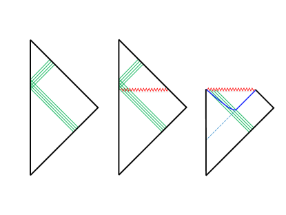
Figure 1: The first figure displays the half Minkowskian plane $x\geq 0$. The axis is located along the left timelike boundary of the figure at $x=0$. The two other boundaries are past and future null infinity. The lines represent the support of the matter field and its reflection off the axis in accord with Equation (3.13). In the second figure, gravity is turned on and a singularity, depicted by the wavy line, forms as soon as the first strand of matter hits the axis so that the reflected stream is cut out of the physical spacetime. The physical spacetime is the Vaidya solution depicted in the third figure. The event horizon is along the dotted line. An apparent horizon (bold line) forms at the left end of the singularity and follows the event horizon after matter collapse. Matter infall is along the unbroken null lines from past null infinity to the singularity.

From (i) and (ii) above, a solution to the classical equations (3.6)- (3.8) is the Vaidya solution with stress energy tensor $T_{++}=\frac{1}{4\pi R^{2}}(\frac{\partial_{+}f)^{2}}{2}$. Since the spacetime geometry in this solution is flat in a finite neighborhood of the axis, the Vaidya solution satisfies our axis requirements. As shown below, it also satisfies the initial conditions at $\cal I^{-}$. Hence it is an acceptable solution.

The Vaidya solution is usually presented in Eddington Finkelstein coordinates $(v,R)$ whereas here we use null coordinates. The relation between the Eddington Finkelstein (EF) and null coordinates is as follows (the reader may find it easier to follow our argumentation below by consulting the Penrose diagram for the Vaidya spacetime depicted in Figure 1.

Consider the Vaidya solution for a mass profile $m(v)$ at $\cal I^{-}$. In EF coordinates $(v,R)$ the 2-metric is:

$${}^{(2)}ds^{2}=-(1-\frac{2m(v)}{R})(dv)^{2}+2dvdR$$ (3.14)

with constant $v$ radial lines being null and ingoing. These ingoing light rays originate at $\cal I^{-}$ of the Vaidya spacetime where $R\rightarrow\infty$. These light rays ‘reflect’ off the axis and become outgoing. Since every outgoing ray originates at the axis as the reflection of a uniqie incoming ray, we can uniquely label each outgoing ray by the value of $v=v_{axis}:=u$ at this origin point on the axis. Thus constant $u$ light rays are outgoing, constant $v$ light rays are incoming and every point in Vaidya spacetime is uniquely located as the intersection of a pair of such rays. This implies that $u,v$ are null coordinates. We now show that the identifications $v\equiv x^{+},u\equiv x^{-}$ hold.

From (3.14) it follows that on an outgoing light ray, $R$ changes as a function of $v$ according to

$$2\frac{dR}{dv}=(1-\frac{2m(v)}{R}).$$ (3.15)

Consider the outgoing ray which starts from the axis at $v=v_{axis}$. As discussed above, we set $v_{axis}=u$. Since $R=0$ at the axis, we may integrate (3.15) to obtain, for the trajectory of this ray:

$$2R(v,u)=\int_{u}^{v}d{\bar{v}}(1-\frac{2m({\bar{v}})}{R({\bar{v}},u)}).$$ (3.16)

Let the support of $m(v)$ start on $\cal I^{-}$ at $v=v_{i}$. Then for $v<v_{i}$, (3.16) implies that:

$$R(v,u)=\frac{v-u}{2}$$ (3.17)

so that the axis lies at:

$$v=u$$ (3.18)

Note that we can rewrite (3.16) as:

$$2R(v,u)=v_{i}-u+\int_{v_{i}}^{v}d{\bar{v}}(1-\frac{2m({\bar{v}})}{R({\bar{v}},u)}).$$ (3.19)

In this form it is clear that the integrand (and hence the equation) is well defined everywhere except at the $R=0$ singularity.

Next, note that since $\cal I^{-}$ is approached as $R\rightarrow\infty$ along constant $v$, it follows from (3.16) that near $\cal I^{-}$:

$$R(v,u)=\frac{v-u}{2}+O(\frac{1}{R})$$ (3.20)

so that $\cal I^{-}$ is approached as $u\rightarrow-\infty$. In this limit, (3.16) implies that:

$$R(v,u)=\frac{v-u}{2}+O(\frac{1}{u})$$ (3.21)

Next, note that setting $R=R(v,u)$ in (3.14), we have

$${}^{(2)}ds^{2}=-(1-\frac{2m(v)}{R})(dv)^{2}+2dv(R,_{v}dv+R,_{u}du)=[-(1-\frac{2m(v)}{R})+2R,_{v}](dv)^{2}+R,_{u}2dvdu$$ (3.22)

which in conjunction with (3.15) implies that in these coordinates the conformal factor $e^{2\rho}$ is given by:

$$2R,_{u}=:-e^{2\rho}$$ (3.23)

From (3.21) and (3.23) it follows that

$$-{2R,_{u}}=1+O(\frac{1}{u^{2}}):=e^{2\rho}$$ (3.24)

Note that from (3.16) we have that:

$$(R,_{u}),_{v}=\frac{m(v)}{2R^{2}}R,_{u}.$$ (3.25)

Since from (3.17) $R,_{u}<0$ at the axis , (3.25) ensures that $R_{u}$ remains negative on every outgoing ray, and hence, negative everywhere so that the identification (3.24) is consistent with the postivity of $e^{2\rho}$.

The above analysis shows that $v,u$ are well defined null coordinates for which the axis conditions (3.18) and ‘initial’ conditions (3.21), (3.24) are satisfied. Further, the geometry in the vicinity of the axis is flat and hence non-singular. Hence we may identify $v$ with $x^{+}$ and $u$ with $x^{-}$, and (from the definition of $m(v)$ for Vaidya spacetime) the mass function $m(v)$ as:

$$m(v)=m(x^{+})=\int_{x^{+}_{i}}^{x^{+}}d{\bar{x}^{+}}\frac{(\partial_{+}f)^{2}}{2}$$ (3.26)

identical to (2.9) where the support of $f(x^{+})$ in the above equation is between $v_{i}\equiv x^{+}_{i}$ and $x^{+}_{f}$. As a final consistency check, note that from (3.25), (3.23) we have that

$$2\rho,_{+}=\frac{m(x^{+})}{2R^{2}},$$ (3.27)

which in conjunction with (3.15), (3.16) and (2.9) suffice to verify that equations (3.6)-(3.8) are satisfied.

4 The semiclassical theory

4.1 Quantization of the matter field

Since the matter field satisfies the free wave equation on the fiducial flat spacetime subject to reflecting boundary conditions at $x=0$ it can be quantized with mode expansion:

$${{\hat{f}}(x^{+},x^{-})}=\int_{0}^{\infty}dk\frac{\cos kx}{\sqrt{\pi k}}({\hat{a}}(k)e^{-ikt}+{\hat{a}}^{\dagger}(k)e^{ikt}).$$ (4.1)

Defining

$${\hat{f}}_{({{+}})}(x^{+}) := {\int_{0}^{\infty}dk\frac{1}{\sqrt{4\pi k}}({\hat{a}}(k)e^{-ikx^{+}}+{\hat{a}}^{\dagger}(k)e^{ikx^{+}})}$$ (4.2)

$${\hat{f}}_{(-)}(x^{-}) := {\int_{0}^{\infty}dk\frac{1}{\sqrt{4\pi k}}({\hat{a}}(k)e^{-ikx^{-}}+{\hat{a}}^{\dagger}(k)e^{ikx^{-}})}$$ (4.3)

we may rewrite (4.1) as

$${{\hat{f}}(x^{+},x^{-})}={{\hat{f}}_{(+)}(x^{+})}+{{\hat{f}}_{(-)}(x^{-})}.$$ (4.4)

Note that the operator valued distribution ${\hat{f}}_{(+)}$ is the same ‘operator valued function’ of its argument as ${\hat{f}}_{(-)}(x^{-})$. This is exactly the quantum implementation of the reflecting boundary condition (3.13)

The mode operators ${\hat{a}}(k),{\hat{a}}^{\dagger}(k)$ provide a representation of the classical symplectic structure which follows from the matter action (3.4) so that the only non-trivial commutation relations are the standard ones:

$$[{\hat{a}}(k),{\hat{a}}^{\dagger}(l)]=\hbar\delta(k,l),$$ (4.5)

which are represented via the standard Fock space representation so that the Hilbert space ${\cal H}_{Fock}$ is the standard Fock space generated by the action of the creation operators ${\hat{a}}^{\dagger}(k)$ on the Fock vacuum.

This quantization may be used to define a test quantum field on the classical Vaidya solution, or to define a quantum field on a general spherically symmetric metric of the form (2.1) or, as we propose in section 6, to define a quantization of the true degrees of freedom of the combined matter-gravity system.

If we use it to define a 4d spherically symmetric test quantum field (coupled to the 4 metric as in (3.3), hence conformally coupled to the 2-metric ${}^{(2)}g$) on the Vaidya spacetime, one can put the test scalar field in its vacuum state at $\cal I^{-}$ and ask for its particle content as experienced by inertial observers at $\cal I^{+}$. A straightforward calculation along the lines of Hawking’s [3] leads to the Hawking effect i.e. the state at $\cal I^{+}$ exhibits late time thermal behavior at Hawking temperature $\frac{1}{8\pi M}$. The calculation is simpler than Hawking’s as, due to the 2d conformal coupling, there is no scattering of particles off the spacetime curvature and hence no non-trivial grey body factors.

If we use the quantization to define a 4d spherically symmetric quantum field (coupled to the 4 metric as in (3.3), hence conformally coupled to the 2-metric ${}^{(2)}g$) on a general spherically symmetric metric (2.1), (2.2), we can compute its stress energy tensor expectation value using the results of Davies and Fulling [7]. Note that since the axis serves as a reflecting boundary and since its trajectory is that of a straight line in the inertial coordinates of the fiducial flat spacetime, the results of Reference [7] can be directly applied.

Recall from [7] that in the case that the initial state at $x^{-}\rightarrow-\infty$ is a coherent state in ${\cal H}_{Fock}$ modelled on a classical field $f$, the vacuum contribution to the stress energy expectation value gets augmented by the classical stress energy of $f$. Recall (see footnote 3) that the $x^{\pm}$ coordinates are freely falling at $\cal I^{-}$ so that the initial state is a coherent state as seen by freely falling observers at $\cal I^{-}$. Putting all this together we have, from [7] that the only non-trivial components of the 4d stress energy expectation value are given through the expressions

$$8\pi R^{2}<{\hat{T}}_{+-}> = -\frac{\hbar}{12\pi}\partial_{+}\partial_{-}\rho$$ (4.6)

$$8\pi R^{2}<{\hat{T}}_{\pm\pm}> = (\partial_{\pm}f)^{2}-\frac{\hbar}{12\pi}((\partial_{\pm}\rho)^{2}-\partial_{\pm}^{2}\rho)$$ (4.7)

The factors of $8\pi R^{2}$ come from the definition of the 4d stress energy (see (3.9)). In general the expressions in (4.7) would be augmented by functions $t_{\pm}(x^{\pm})$ which are state dependent. Here, these vanish because the mode expansion (4.1) is defined with respect to the $x^{\pm}$ coordinates [7].

4.2 Semiclassical Equations

The semiclassical Einstein equations find their justification in the large $N$ approximation [8]. Accordingly we couple $N$ scalar fields exactly as in (3.3), quantize each of them as in the previous section, put one of them in a coherent state modelled on $f$ and the rest in their vacuum states at $\cal I^{-}$. From (4.6), (4.7) and (3.6)-(3.8), it then follows that the semiclassical Einstein equations, $G_{ab}=8\pi\langle T_{ab}\rangle$ take the form:

$$-\frac{e^{2\rho}}{4}G_{{\hat{\Omega}}{\hat{\Omega}}} = \partial_{+}\partial_{-}\rho+\frac{1}{R}\partial_{+}\partial_{-}R=0$$ (4.8)

$$R^{2}\;G_{+-} = 2R\partial_{+}\partial_{-}R+2\partial_{+}R\partial_{-}R+\frac{1}{2}e^{2\rho}=-\frac{N\hbar}{12\pi}\partial_{+}\partial_{-}\rho$$ (4.9)

$$R^{2}\;G_{\pm\pm} = R^{2}[-\frac{2}{R}(\partial_{\pm}^{2}R-2\partial_{\pm}\rho\partial_{\pm}R)]=(\partial_{\pm}f)^{2}-\frac{N\hbar}{12\pi}((\partial_{\pm}\rho)^{2}-\partial_{\pm}^{2}\rho)$$ (4.10)

4.3 Semiclassical Singularity

We are interested in semiclassical solutions in which the axis is located at $x=0$, the axial geometry is non-singular and for which the asymptotic conditions (2.6) hold. Note that when $\rho=0$ the vacuum fluctuation contribution to the stress energy expectation value vanishes. Thus, when $f$ vanishes, classical flat spacetime (with $e^{2\rho}=1,R=\frac{x^{+}-x^{-}}{2}$) remains a solution. Hence for $x^{+}<x^{+}_{i}$ we set the spacetime to be flat with

$$e^{2\rho}=1,\;\;\;R=\frac{x^{+}-x^{-}}{2}$$ (4.11)

Next, note that we can eliminate $\partial_{+}\partial_{-}\rho$ between the first two eqns to obtain:

$$\frac{1}{R}\partial_{+}\partial_{-}R=-\frac{\partial_{+}R\partial_{-}R+\frac{1}{4}e^{2\rho}}{R^{2}-{\frac{N\hbar}{24\pi}}}$$ (4.12)

Following Lowe [1] and Parentani and Piran [2], we can look upon (4.12), (3.6) as evolution equations for initial data (i) on the null line $x^{+}=x^{+}_{i}$ and (ii) on $\cal I^{-}$ for $x\geq x^{+}_{i}$ . For (i) , the initial data is given by (4.11). For (ii), the matter data is subject to (2.10) and the gravitational data corresponds to that for the Vaidya solution with $m(x^{+})$ given by (2.9) and $R,\rho$ obtained by integrating (3.15) along $\cal I^{-}$ and then using (3.23). More in detail, at $x^{+}=x^{+}_{i}$, we have data near $\cal I^{-}$ of the form (4.11). Equation (3.15) can be integrated along $\cal I^{-}$ with this initial data for $R$ to obtain $R$ along $\cal I^{-}$ for $x\geq x^{+}$ and $e^{2\rho}$ can then be obtained near $\cal I^{-}$ from (3.23). It can then be shown that the evolution equations can be solved uniquely for $R,\rho$ in the region $x^{+}\geq x^{+}_{i}$ as long as the evolution equations themselves are well defined.

From a numerical evolution point of view [1] one can see this as follows. Along $x^{+}=x^{+}_{i}$, equation (4.12) can be viewed as a first order differential equation for $R,_{+}$ on $x^{+}=x^{+}_{i}$ with ‘inital’ value for $R,_{+}$ specified on $\cal I^{-}$ and known coefficients from (4.11). The solution $R,_{+}(x^{+}=x^{+}_{i},x^{-})$ together with initial value for $\rho,_{+}$ on $\cal I^{-}$ can be used to solve (3.6) for $\rho,_{+}$ on the line $x^{+}=x^{+}_{i}$. From this one has data $\rho,R$ for the next $x^{+}$=constant=$x^{+}_{i}+\epsilon$ line on the numerical grid and the procedure can be iterated so as to eventually cover all of $x^{+}>x^{+}_{i}$..

We now argue that for generic matter data the evolution equations break down at $R^{2}={\frac{N\hbar}{24\pi}}$ and a curvature singularity develops. In this regard note that the denominator of the right hand side of (4.12) blows up at $R^{2}={\frac{N\hbar}{24\pi}}$. If the numerator is non-zero at this value of $R$ the left hand side blows up and through (3.6) so does $\partial_{+}\partial_{-}\rho$. Since (as can be easily checked), ${}^{(2)}R=8e^{-2\rho}\partial_{+}\partial_{-}\rho$ we expect a 2-curvature singularity at this value of $R^{2}$. If the numerator vanishes at some $x^{+}=a^{+}>x^{+}_{i},x^{-}=a^{-}$ where $R^{2}(a^{+},a^{-})={\frac{N\hbar}{24\pi}}$, one can slightly change the initial data for $f$ on $\cal I^{-}$, thereby change the function $R$ along $\cal I^{-}$ (for $x^{+}>x^{+}_{i}$) and hence the ‘initial’ data $R,_{+}$ for (4.12) at $x^{+}=a^{+}$ on $\cal I^{-}$. This would generically result in a change of the numerator away from zero. Thus one expects that for generic matter data there is a singularity at $R^{2}={\frac{N\hbar}{24\pi}}$.

Thus the ‘initial point’ of the Vaidya singularity of the classical theory moves ‘downwards’ along the initial matter infall line $x^{+}=x^{+}_{i}$ away from the axis where $R=0$ to $R=\sqrt{{\frac{N\hbar}{24\pi}}}$ (see Figure 2.

4.4 Outer Marginally Trapped Surfaces

One possible quasilocal characterization of a black hole is the existence of outer marginally trapped surfaces (OMTS’s) [10, 11]. In this section we analyse the behavior of spherically symmetric OMTS’s in the context of the system studied in this work. To this end, fix an $R=$constant 2 sphere. Let the expansions $\theta_{+}$ and $\theta_{-}$ denote the expansions of outward and inward future pointing radial null congruences at this sphere. The sphere is defined to be an OMTS if $\theta_{+}=0,\theta_{-}<0$. A straightforward calculation yields:

$$\theta_{\pm}=2e^{-2\rho}\frac{\partial_{\pm}R}{R}$$ (4.13)

Since the physical spacetimes considered in this work are flat near the axis, such OMTS’s can only form in these solutions away from the axis where $R>0$. Hence (assuming we are away from singularities), the conditions for an OMTS to form are:

$$\partial_{+}R = 0$$ (4.14)

$$\partial_{-}R < 0$$ (4.15)

While an OMTS is a quasilocal characterization of a black hole at an ‘instant of time’and hence a 2-sphere, the quasilocal analog of the 3d event horizon is a 1 parameter family of OMTS’s which form a tube which we call an Outer Marginally Trapped Tube (OMTT). The shape of a spherically symmetric OMTT (i.e. a tube foliated by spherically symmetric OMTS’s) can be studied as follows. Since (4.14) holds, the normal $n_{a}$ to the OMTT is:

$$(n_{+},n_{-})=(\partial_{+}^{2}R,\partial_{-}\partial_{+}R)=(-4\pi R\langle T_{++}\rangle,-\frac{Re^{2\rho}}{4(R^{2}-\frac{\hbar N}{24\pi})})$$ (4.16)

$$\Rightarrow n^{a}n_{a}=-4e^{-2\rho}4\pi R\langle T_{++}\rangle\frac{Re^{2\rho}}{4(R^{2}-\frac{\hbar N}{24\pi})}$$ (4.17)

where we have used the ‘++’ equation in (4.10) with (4.14) to calculate $n_{+}$ and (4.12) with (4.14) to compute $n_{-}$ in (4.16). From (4.17), $n_{a}n^{a}$ is timelike, spacelike or null if $\langle T_{++}\rangle$ is, respectively positive, negative or vanishing so that OMTT is, respectively, spacelike, timelike or null.

Following [12], we coordinatize the trajectory of the spherically symmetric OMTT by $x^{+}$ and study how $x^{-}$ changes with $x^{+}$ along this trajectory. Since $\partial_{+}R$ vanishes along this trajectory we have that:

$$\frac{d\partial_{+}R}{dx^{+}} = \partial_{+}^{2}R+\frac{dx^{-}}{dx^{+}}\partial_{-}\partial_{+}R=0$$

$$\Rightarrow\frac{dx^{-}}{dx^{+}} = -\frac{\partial_{+}^{2}R}{\partial_{-}\partial_{+}R}=-(16\pi e^{-2\rho}(R^{2}-\frac{\hbar N}{24\pi}))\langle T_{++}\rangle$$ (4.18)

where we have used (4.16). Equation (4.18) leads us to the same correlation between positivity properties of the stress energy and the spacelike, timelike or null nature of the OMTT as above.

Next, note that on the OMTT:

$$\frac{dR}{dx^{+}} = \partial_{+}R+\frac{dx^{-}}{dx^{+}}\partial_{-}R$$ (4.19)

$$= (16\pi e^{-2\rho}(R^{2}-\frac{\hbar N}{24\pi}))(-\partial_{-}R)\langle T_{++}\rangle$$

where we have used (4.14) together with (4.18). From (4.15) it follows that $R$ (and hence the area of the OMTS cross section of the OMTT) increases, decreases or is unchanged if, respectively, $\langle T_{++}\rangle$ is positive, negative or null.

The above set of results correspond to those of [11] in the simple spherically symmetric setting of our work. Let us apply them to the following physical scenario. For a large black hole, we expect a low Hawking temperature and rate of thermal emmission. emmission. In the context of the system studied here, consider a black hole of mass $(M^{2}>>N\hbar$ (as we shall see in section 5) the Hawking emmission in a QFT in CS calculation goes as $N\hbar M^{-2}$ at $\cal I^{+}$).

Let us assume that the collapse lasts for a small duration (i.e. $x^{+}_{f}-x^{+}_{i}<<GM$) during which classical infall dominates quantum back reaction at large $R$ (including at $R\sim M$). Once the collapse is over, we expect the black hole to start radiating slowly. We can estimate the local rate of mass loss due to this radiation by assuming the geometry at this epoch is well approximated by the classical Vaidya geometry. More precisely, let us assume that the quantum radiation starts along the line $x^{+}=x^{+}_{f}$ at the 2-sphere at which the event horizon $R=2M$ intersects this line. Since this 2 sphere is an OMTS in the Vaidya spacetime, within our approximation we may apply (4.19) to estimate the rate of change of area of this OMTS with the right hand side calculated using the Vaidya geometry:

$$\frac{dR}{dx^{+}} = (16\pi e^{-2\rho}(R^{2}-\frac{\hbar N}{24\pi}))(-\partial_{-}R)\langle T_{++}\rangle$$ (4.20)

$$\approx (-2\partial_{-}Re^{-2\rho})R^{2}8\pi\langle T_{++}\rangle$$ (4.21)

$$\approx -\frac{N\hbar}{12\pi}((\partial_{\pm}\rho)^{2}-\partial_{\pm}^{2}\rho)$$ (4.22)

where in the second line we used the large black hole approximation $(M^{2}>>N\hbar$ and in the third we used the property (3.23) of the Vaidya spacetime together with equation (4.10). Using (3.27) with $R=2M$, we have $\partial_{+}\rho=\frac{1}{8M^{2}}$ and, using (3.27) together with (3.15) we have $(\partial_{+})^{2}\rho=0$. Putting this in (4.22) and setting $R=2M$ on the left hand side, we obtain

$$\frac{dM}{dx^{+}}=-\frac{N\hbar}{24\pi}\frac{1}{64M^{2}}$$ (4.23)

Remarkably this agrees with rate of mass loss obtained at $\cal I^{+}$ (see (5.19) of section 5). This agreement of quasilocal mass loss with that at $\cal I^{+}$ for large black holes also seems to happen for the case of CGHS black holes [12]. We do not understand the deeper reason behind this agreement.

4.5 The semiclassical spacetime solution: folding in results from prior numerics

While the semiclassical equations do not seem amenable to analytical solution the particular semiclassical solution of interest, with flat geometry in a finite region around the symmetry axis, is amenable to numerical solution along the lines reviewed in section 4.3. While we advocate a careful numerical study along the lines of [13], there are two prior numerical works by Lowe [1] and by Parentani and Piran [2] which are of relevance. While these beautiful works are not cognizant of key aspects of the coherent picture developed in this work, the semiclassical equations they solve are practically the same as those in this work and they provide a key complimentary resource to our work here.

The work by Lowe [1] uses exactly the same action (3.5) (modulo some overall numerical factors) and hence obtains the same semiclassical equations (modulo some numerical factors). Since the importance of the axis and the axis reflecting boundary conditions for the matter field is not realised, the state dependent functions $t^{\pm}(x^{\pm})$ (see the end of section 4.1) are not pre-specified but chosen in accord with the physical situation which is modelled. The ‘classical’ component of matter is chosen to be a shock wave with a Dirac delta stress energy along this infall line (from our point of view the Dirac delta function ensures that the prompt collapse condition (2.10) is satisfied). Along the infall line the data for $R,\rho$ is chosen as $R=\frac{x^{+}_{i}-x^{-}}{2},\rho=0$. Initial conditions at $\cal I^{-}$ beyond the point of matter infall are specified which correspond to the asymptotic behavior of the Schwarzschild solution. These suffice for well defined numerical evolution as described in section 4.3.

One difference with our work here is that these conditions by virtue of the presence of logarithmic terms in metric fall offs at $\cal I^{-}$ [1], do not agree with the conditions (2.6). We believe, contrary to the implicit assertion in Reference [1], that a continuation of the data of [1] on $x^{+}=x^{+}_{i}$ to flat spacetime data $R=\frac{x^{+}_{-}x^{-}}{2},\rho=0$ for $x^{+}<x^{+}_{i}$, is in contradiction with the behavior of the Vaidya solution near $\cal I^{-}$. While it would be good to clarify whether such a continuation is consistent with the Einstein equations near $\cal I^{-}$, this is beyond the scope of our paper. Notwithstanding this, we shall assume that the physics which emerges from the numerical results of [1] is robust enough that it applies to the system studied in this work.

Lowe [1] notes the existence of a spacelike semiclassical singularity and the emanation of an OMTT at the infall line. Since the classical matter is a shock wave with no extended support, quantum backreaction starts immediately and the OMTT is timelike. The OMTT and the singularity meet away from $\cal I^{+}$ in the interior of the space time. The outgoing future pointing radial null rays starting at this intersection form a Cauchy horizon. There is no evidence of a ‘thunderbolt’ along this ‘last’ set of null rays to $\cal I^{+}$. This ‘outer’ Cauchy horizon is in addition to the ‘inner’ Cauchy horizon which forms along the infall line beyond $R^{2}=\frac{\hbar N}{24}$.

Parentani and Piran [2] define the semiclassical equations without recourse to action based arguments by positing the stress energy tensor to be the sum of a classical part and a quantum back reaction part. The former is posited to be of the null dust type infall appropriate to Vaidya. The profile of the dust is chosen to be a Gaussian but in the numerics we are unable to discern if its tail is cut off and if so whether, effectively, the prompt collapse condition (2.10) is satisfied. While the work explicitly recognizes the existence of an axis, its import for the reflecting boundary conditions in the quantization of the scalar field (see section 4.1) is not recognized. The fact that the classical solution is Vaidya and that for a Gaussian profile which is not one of prompt collapse, the classical singularity structure is complicated [6] is not appreciated. The quantum contribution to the stress tensor is chosen to be of exactly the form in (4.9)-(4.10) without the realization that it could arise naturally through quantization of an appropriately chosen classical scalar field as shown in this work.

The solution chosen is, by virtue of ignoring the tail contributions of the Gaussian, in practice flat in a finite neighborhood of the axis so that the dynamical and constraint equations and set up for numerical evolution are exactly the same as Lowe. Since the set up is numerical, initial conditions are at large but finite $x^{-}=x^{-}_{I}$ rather than at $\cal I^{-}$. A coordinate choice of $x^{+}$ which agrees with ours for $x^{+}<x^{+}_{i}$ but differs from ours elsewhere is made. This choice depends on $x^{-}_{I}$ and as $x^{-}_{I}\rightarrow-\infty$ approaches ours. We shall assume that the basic physics is robust with regard to the difference in these choices.

Parentani and Piran note the existence of a spacelike semiclassical singularity at $R^{2}=\frac{\hbar N}{24}$ and a OMTT which is spacelike as long as classical matter infall dominates after which it turns timelike and meets the singularity away from $\cal I^{+}$. Similar to [1] a Cauchy horizon then forms. Interestingly, the quantum flux at $\cal I^{+}$ starts out as thermal flux at temperature inversely proportional to the initial mass, its mass dependence being $\sim M^{-2}$ as expected. However at late stages of evaporation, near the intersection of $\cal I^{+}$ with the Cauchy horizon, where the Bondi mass gets small, the flux turns around to a less divergent function of this small mass . We take this as evidence for lack of a thunderbolt.

Putting together (i) the analytical work of sections 4.3, 4.4, (ii) the physical intuition that the initial part of spacetime is dominated by classical collapse followed by quantum radiation and (iii) the beautiful numerical work of References [1, 2], we propose the Penrose diagram in Fig 2 as a description of the semiclassical spacetime geometry.

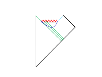
Figure 2: The figure depicts the proposed semiclassical spacetime solution. Towards the left of the initial matter infall line, the spacetime is flat. The singularity, depicted by a wavy line, starts along this infall line and is located away from the axis at $R=\sqrt{\frac{N\hbar}{24}}$. A spacelike apparent horizon is born at the left end of the singularity and grows as long as the classical stress energy dominates the quantum contribution. Once the back reaction dominates the effect of the classical matter stress energy, the apparent horizon turns upwards into a timelike marginally trapped tube which meets the singularity. A Cauchy horizon forms along the last rays which originate at this meeting point and travel to $\cal I^{+}$. There is also a Cauchy horizon between the left end of the singularity and the axis.

5 A balance law at $\cal I^{+}$

We make two assumptions regarding the asymptotic behavior of the metric at $\cal I^{+}$:

A1. We expect that at early times at $\cal I^{+}$ back reaction effects have not built up and that the classical ingoing Vaidya solution discussed in section 3 is a good approximation to the spacetime geometry.

A2. We expect that eventually back reaction effects build up and produce a non-trivial stress energy flux at $\cal I^{+}$. Since the system is spherical symmetric we assume that this situation can be modelled by an outgoing Vaidya metric all along $\cal I^{+}$. Thus the metric near $\cal I^{+}$ is assumed to take the form:

$${}^{(2)}ds^{2}=-(1-\frac{2m_{B}(\bar{u})}{R})(d{\bar{u}})^{2}-2d\bar{u}dR+O(\frac{1}{R^{2}}).$$ (5.1)

Here $R\rightarrow\infty$, $\bar{u}$ is an Eddington-Finkelstein null coordinate and the subscript $B$ on the outgoing mass indicates that this mass is the Bondi Mass.

From A1, at early times, $\cal I^{+}$ is located at $x^{+}=\infty$. Since $\cal I^{+}$ is null, we shall assume that at all times, it is located at $x^{+}=\infty$. Since $\bar{u}$ is an outgoing null coordinate, the 2-metric (5.1) near $\cal I^{+}$ can be expressed in conformally flat form in the coordinates $x^{+},\bar{u}$ as:

$${}^{(2)}ds^{2}=-e^{2\bar{\rho}}dx^{+}d\bar{u}$$ (5.2)

Similar to (3.27), to leading order in $\frac{1}{R}$, it follows that

$$\frac{\partial}{\partial\bar{u}}\bar{\rho}(x^{+},\bar{u})=O(\frac{1}{R^{2}})\;\;\;\;\;\frac{\partial^{2}}{\partial\bar{u}^{2}}\bar{\rho}(x^{+},\bar{u})=O(\frac{1}{R^{2}})$$ (5.3)

Since $\bar{u},x^{-}$ are both outgoing null coordinates, the coordinate $\bar{u}$ is a function only of $x^{-}$ and not $x^{+}$. Using this fact together with the ‘$--$’ constraint (4.10), the asymptotic form (5.2) and the behavior of the conformal factor (5.3), it is straightforward to show that at $\cal I^{+}$ in the limit $R\rightarrow\infty$:

$$-\frac{1}{2}R^{2}G_{{\bar{u}}{\bar{u}}} = \frac{dm_{B}}{d{\bar{u}}}$$ (5.4)

$$= -4\pi R^{2}\langle{\hat{T}}_{\bar{u}\bar{u}}\rangle$$ (5.5)

$$= -{\frac{1}{2}(\partial_{\bar{u}}f)^{2}}+\frac{N\hbar}{48\pi}(\frac{1}{{\bar{u}}^{\prime}})^{2}[\frac{3}{2}(\frac{{\bar{u}}^{\prime\prime}}{{\bar{u}}^{\prime}})^{2}-\frac{{\bar{u}}^{\prime\prime\prime}}{{\bar{u}}^{\prime}}]$$ (5.6)

where each ‘$\prime$’ superscript signifies a derivative with respect to $x^{-}$ so that, for e.g. $\bar{u}^{\prime}:=\frac{d\bar{u}}{dx^{-}}$. Thus we have derived a balance law relating the change of Bondi mass (with respect to the asymptotic translation in $\bar{u}$ along $\cal I^{+}$) to the energy flux at $\cal I^{+}$:

$$\frac{dm_{B}}{d{\bar{u}}}=-{\frac{1}{2}(\partial_{\bar{u}}f)^{2}}+\frac{N\hbar}{48\pi}(\frac{1}{{\bar{u}}^{\prime}})^{2}[\frac{3}{2}(\frac{{\bar{u}}^{\prime\prime}}{{\bar{u}}^{\prime}})^{2}-\frac{{\bar{u}}^{\prime\prime\prime}}{{\bar{u}}^{\prime}}]:=-{\cal F}$$ (5.7)

The energy flux ${\cal F}$ has a ‘classical’ part ${\cal F}^{classical}$ (about which we shall comment in the next section) corresponding to the first term on the right hand side of (5.7) and a quantum backreaction part ${\cal F}^{quantum}$ corresponding to the rest of the right hand side of (5.7):

$${\cal F} = {\cal F}^{classical}+{\cal F}^{quantum}$$ (5.8)

$${\cal F}^{classical} = {\frac{1}{2}(\partial_{\bar{u}}f)^{2}}$$ (5.9)

$${\cal F}^{quantum} = -\frac{N\hbar}{48\pi}(\frac{1}{{\bar{u}}^{\prime}})^{2}[\frac{3}{2}(\frac{{\bar{u}}^{\prime\prime}}{{\bar{u}}^{\prime}})^{2}+\frac{{\bar{u}}^{\prime\prime\prime}}{{\bar{u}}^{\prime}}]$$ (5.10)

While the classical piece is explicitly positive definite, this property does not hold for the quantum piece. However, following [4], we can rewrite this quantum part as:

$${\cal F}^{quantum} = -\frac{N\hbar}{48\pi}(\frac{1}{{\bar{u}}^{\prime}})^{2}[\frac{3}{2}(\frac{{\bar{u}}^{\prime\prime}}{{\bar{u}}^{\prime}})^{2}-\frac{{\bar{u}}^{\prime\prime\prime}}{{\bar{u}}^{\prime}}]$$ (5.11)

$$= \frac{d}{d{\bar{u}}}[{\frac{N\hbar}{48\pi}(\frac{{\bar{u}}^{\prime\prime}}{({\bar{u}}^{\prime})^{2}}}]+\frac{N\hbar}{96\pi}\frac{({\bar{u}}^{\prime\prime})^{2}}{({\bar{u}}^{\prime})^{4}}.$$ (5.12)

Using (5.12) we may rewrite (5.7) as:

$$\frac{d}{d{\bar{u}}}[m_{B}+{\frac{N\hbar}{48\pi}(\frac{{\bar{u}}^{\prime\prime}}{({\bar{u}}^{\prime})^{2}}}]=-{\frac{1}{2}(\partial_{\bar{u}}f)^{2}}-\frac{N\hbar}{96\pi}\frac{({\bar{u}}^{\prime\prime})^{2}}{({\bar{u}}^{\prime})^{4}}.$$ (5.13)

The right hand side of (5.13) is now explicitly negative definite. Equation (5.13) suggests that we identify the term in square brackets on its left hand side as a back reaction corrected Bondi mass $m_{B,corrected}$,

$$m_{B,corrected}:=m_{B}+{\frac{N\hbar}{48\pi}\frac{{\bar{u}}^{\prime\prime}}{({\bar{u}}^{\prime})^{2}}},$$ (5.14)

which decreases in response to the outgoing positive definite back reaction corrected flux ${\cal F}_{corrected}$ received at $\cal I^{+}$ :

$${\cal F}_{corrected}:={\frac{1}{2}(\partial_{\bar{u}}f)^{2}}+\frac{N\hbar}{96\pi}\frac{({\bar{u}}^{\prime\prime})^{2}}{({\bar{u}}^{\prime})^{4}}.$$ (5.15)

The form of the back reaction corrected balance law (5.13) suggests that black hole evaporation ceases when the corrected Bondi mass $m_{B,corrected}$ (5.14) is exhausted, at which point the corrected flux ${\cal F}_{corrected}$ (5.15) also vanishes. For ${\cal F}_{corrected}$ to vanish both its ‘classical’ and quantum contributions must vanish seperately since both are positive definite. In particular the quantum contribution ${\cal F}^{quantum}_{corrected}$ must vanish so that:

$${\cal F}^{quantum}_{corrected}:=\frac{N\hbar}{96\pi}\frac{({\bar{u}}^{\prime\prime})^{2}}{({\bar{u}}^{\prime})^{4}}=0$$ (5.16)

Assuming that this happens smoothly, it must be the case that:

$${\bar{u}}^{\prime\prime}=0$$ (5.17)

which implies that $\bar{u}$ is a linear function of $x^{-}$:

$$\bar{u}=ax^{-}+b$$ (5.18)

for some constants $a,b$. Since $\bar{u}$ is a future pointing null coordinate, we have that $\bar{u}^{\prime}>0$ and hence, $a>0$. This implies that as $\bar{u}\rightarrow\infty$, $x^{-}\rightarrow\infty$ which means that $\cal I^{+}$ of the physical spacetime is ‘as long’ as that of the fiducial Minkowski spacetime. Note that in contrast the $\cal I^{+}$ of Vaidya ends at $x^{-}=x^{-}_{H}$ where $x^{-}_{H}$ is the (finite) value of $x^{-}$ at the horizon. In this sense $\cal I^{+}$ of the physical spacetime is ‘quantum’ extended beyond its classical counterpart. This is the main conclusion of this section. We discuss its possible implications in the next section where we also discuss the origin of the ‘classical’ contribution to ${\cal F}$.

Before doing so, we note that it is possible to calculate the flux ${\cal F}$ (5.8) at $\cal I^{+}$ of the Vaidya spacetime with $\rho$ corresponding to that of the Vaidya solution. Recall from section 3 that in the Vaidya solution the outgoing classical flux is absent. As shown in the Appendix C, the quantum flux ${\cal F}^{quantum}$ evaluates at late times on $\cal I^{+}$ of the Vaidya spactime to:

$${\cal F}^{quantum}=\frac{N\hbar}{24\pi}(\frac{1}{64M^{2}})$$ (5.19)

We can also calculate the corrected quantum flux ${\cal F}^{quantum}_{corrected}$

$${\cal F}^{quantum}_{corrected}:=\frac{N\hbar}{96\pi}\frac{({\bar{u}}^{\prime\prime})^{2}}{({\bar{u}}^{\prime})^{4}}$$ (5.20)

and as shown in Appendix C this agrees with ${\cal F}^{quantum}$ at late times i.e. at late times,

$${\cal F}^{quantum}_{corrected}={\cal F}^{quantum}=\frac{N\hbar}{24\pi}(\frac{1}{64M^{2}})$$ (5.21)

Equation (5.21) corresponds to the thermal Hawking flux measured at $\cal I^{+}$ in the quantum field theory on curved spacetime approximation.

6 Speculations on the deep quantum behavior of the system

We propose that the true degrees of freedom of the system (3.5) are those of the scalar field and that the gravitational degrees of freedom can be solved for in terms of specified matter data (classically) or when the quantum state of matter is specified (semiclassically and at the deep quantum gravity level). This proposal is supported by the fact that in the classical theory if we set the matter field to vanish, flat spacetime is the unique classical solution to equations (3.6)- (3.8) subject to asymptotic flatness at past null infinity (2.6) as well as the condition that the axis of symmetry exist and be located at (2.5). Clearly, the proposal would be on a firmer footing if for the classical and semiclassical equations, we could prescribe precise boundary conditions on the geometry variables $\rho,R$ at the axis together with the initial conditions (2.6) such that a specification of matter data at $\cal I^{-}$ subject to reflecting boundary conditions at the axis (as discussed in section 2.2), results in a unique solution. While a complete treatment is beyond the scope of this paper, in anticipation of future work towards such a treatment, we initiate an analysis of possible boundary conditions at the axis in Appendix A and comment on the complications which arise due to its timelike nature.

Notwithstanding the remarks above, let us go ahead and assume that the true degrees of freedom at the classical level are those of the classical scalar field data at $\cal I^{-}$ and that, correspondingly, the true quantum degrees of freedom of the gravity-matter system are those of the quantum scalar field. This implies that the Hilbert space for the quantum gravity-matter system is the Fock space ${\cal H}_{Fock}$ constructed in section 4.1 and that the natural arena for these degrees of freedom is the Minkowkskian half plane $x\geq 0$. This assumption is supported by the considerations of section 5 wherein we argued that the physical $\cal I^{+}$ was as long as the fiducial Minkowskian $\cal I^{+}$.

More in detail the starting point for this argument in section 5 is an assumed validity of the semiclassical equations at $\cal I^{+}$. These equations via the arguments of [8] relate the Einstein tensor of the expectation value of the metric to the expectation value of the stress energy tensor and are assumed to hold when the quantum fluctuations of the geometry are negligible. Hence, while the semiclassical equations are not expected to hold near the singularity where geometry fluctuations are expected to be significant, it seems reasonable to assume that they do hold near $\cal I^{+}$. If they do hold near $\cal I^{+}$ (assuming, of course that the expectation value geometry is asymptotically flat), then the reasonable assumptions of section 5 lead to the conclusion of a quantum extended $\cal I^{+}$ which is as long as the fiducial Minkowskian $\cal I^{+}$; this conclusion is supportive of the idea that the correct physical arena is the half Minkowskian plane.

Note also that the proposed true degrees of freedom, namely those of the quantum scalar field, propagate on the fiducial flat spacetime by virtue of their 2d conformal coupling. Hence these degrees of freedom admit well defined propagation through the semiclassically singular region. The infalling quantum scalar field is reflected off the axis transmuting thereby to the outgoing scalar field which registers on the quantum extension of $\cal I^{+}$. This is the origin of the ‘classical’ contribution (5.9) to the asymptotic flux of section 5.

Since quantum evolution of the true (matter) degrees of freedom of the system is well defined even at classically or semiclassically singular regions, one might hope that it is possible to define the action of operator correspondents of gravitational variables in these regions as well. In this sense one may hope that the deep quantum theory resolves the singularities of the classical/semiclassical theory.

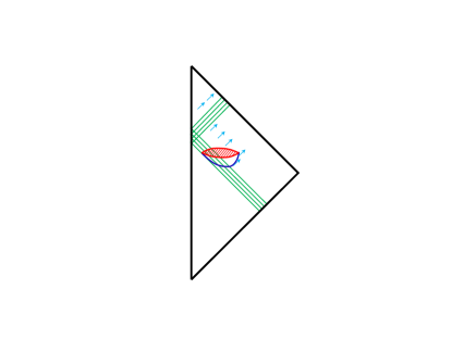
Figure 3: The figure depicts the quantum extended spacetime manifold which coincides with the half Minkowskian plane. The oval striped region indicates the semiclassically singular region which is resolved at the deep quantum level. In this part of the manifold , spacetime geometry fluctuations are large and there is no clear notion of causality. A vast region of spacetime opens up beyond this hitherto singular region. The classical matter field, depicted by unbroken lines, passes through this region, is reflected off the axis and arrives at the extend $\cal I^{+}$. The arrows correspond to outgoing quantum stress energy.

From the above, admittedly speculative, discussion we are lead to the spacetime picture depicted in Figure 3 This picture is reminiscent of the Ashtekar Bojowald paradigm [5] wherein gravitational singularities are assumed to be resolved by quantum gravity effects, the classical spacetime admits a quantum extension and quantum correlations with earlier thermal Hawking radiation emerge in this quantum extension. Since, in the spacetime picture of Figure 3 the quantum extended spacetime arena is exactly the Minkowskian half plane, we do expect the quantum state at its $\cal I^{+}$ to be pure. However it is not clear if the state lies in the same Hilbert space ${\cal H}_{Fock}$ as the initial coherent state on $\cal I^{-}$.

Preliminary calculations suggest that if $\bar{u}(x^{-})$ is sufficiently smooth and approaches $x^{-}$ as $x^{-}\rightarrow\pm\infty$ sufficiently fast the relevant Bogoliuibov transformation between freely falling modes at $\cal I^{-}$ and $\cal I^{+}$ suffers from no ultraviolet divergences. There seem, however, to be infra-red divergences. Infrared divergences are typical of massless field theory in 1+1 dimensions and require a more careful treatment [14]. As indicated in [15], it is possible that such a treatment may lead to the conclusion that it is only ultraviolet divergences which are an obstruction to the unitary implementability of the Bogoliubov transformation. If so, we would expect that under the above conditions on $\bar{u}$, not only is the quantum state on $\cal I^{+}$ pure, it is also in the same Hilbert space ${\cal H}_{Fock}$ as the initial coherent state on $\cal I^{-}$. Note that if $a=1$ in (5.18), then provided $\bar{u}(x^{-})$ is sufficiently smooth and approaches $x^{-}$ as $x^{-}\rightarrow-\infty$ sufficiently fast, the above discussion applies. For the case $a\neq 1$ we are unable to make any statement and we leave this case (as well as a confirmation of our preliminary calculations for the $a=1$ case) for future work. If the state at $\cal I^{+}$ is not in ${\cal H}_{Fock}$, we may still interpet it as an algebraic (and presumably pure) state from the perspective of the algebraic approach to quantum field theory [16].

7 Discussion

In light of the discussion of section 6, we expect that the state at $\cal I^{+}$ is pure. We expect that at early times, the state at $\cal I^{+}$ is a mixed state of slowly increasing Hawking temperature. Hence it is of interest to understand how this state is purified to one on extended $\cal I^{+}$. Directly relevant tools to explore this question have been developed in the recent beautiful work of Agullo, Calizaya Cabrera and Elizaga Navascues [17]. Envisaged work consists in a putative application of their work to the context of the system studied in this paper. Another question of physical interest concerns the classically/semiclassically singular region. While the quantum fluctuations of geometry are expected to be large in this region, it might still be possible to describe the expectation value geometry through an effective metric. In this regard, the setting for the arguments of [18] seem to be satisfied so that it might be possible to argue that the semiclassical singularity is mild in the sense that the conformal factor is continuous at this singularity. It might then be possible to continue it past the singularity along the lines of [18] and compare the resulting geometry to existing proposals in the literature such as [19, 20, 21].

It would also be of interest to understand the semiclassical solution numerically, especially with regard to the behavior of the spacetime geometry and stress energy along the last set of rays from the intersection of the marginally trapped tube and the singularity to $\cal I^{+}$. In the closely related semiclassical theory of the 2d CGHS model, there is a last ray from exactly such an intersection and extremely interesting universality in quantities such as the Bondi mass and Bondi flux (scaled down by $N$) at the last ray [13]. This universality holds if the black hole formed by collapse is sufficiently large in a precisely defined sense. An investigation of physics and possible universality along the last set of rays in the system studied in this work is even more interesting given that, in contrast to the CGHS case in which the Hawking temperature is independent of mass, the Hawking temperrature here has the standard inverse mass dependence. As far as we can discern, the black holes studied by Parentani and Piran [2] are microscopic; it would be exciting if the turn over to less singular behavior in the flux near the last rays seen by them holds also for initially large black holes.

Appendices

Appendix A Comments on Axis Boundary Conditions

Note that the geometry in the vicinity of the axis is, by definition of the axis, non-singular. As shown in the next section A.1 the requirement of non-singularity at the axis is quite powerful and constrains the behavior of $\rho,R$ at the axis as folows:

$$R=0\;\;\;\;\;\;\partial_{x}R=e^{\rho}\;\;\;\;\;\;\;\;\;\partial_{x}\rho=0$$ (A.1)

$$\partial_{x}^{2}R=0$$ (A.2)

In order to obtain these results we assume, in addition to the requirement of non-singular geometry near the axis, that $x^{\pm}$ is a good coordinate system for the 2 geometry defined by ${}^{(2)}g$. Specifically we assume that:
(a) The coordinate vector fields $\big{(}\frac{\partial}{\partial x^{\pm}}\big{)}^{a}$ are well behaved everywhere and in particular near and at the axis.
(b) The conformal factor $e^{2\rho}$ is finite and non-vanishing
(c) In the timelike distant past (i.e as $t\rightarrow-\infty$), the metric is flat with $\rho\rightarrow 0$, $R\rightarrow x$.

In section A.1 we interpret the requirement of non-singular axial geometry as the finiteness of ${}^{(4)}R,{}^{(2)}R$ and $G_{ab}v^{a}w^{b}$ (for all well behaved vector fields $v,w$). It is possible that additional conditions are implied by a similar requirement of finiteness of the Weyl tensor. We leave the relevant analysis for future work.

Due to the timelike nature of the axis, we are not sure if the entire set of conditions (A.1)- (A.2) can be consistently imposed. More in detail, from the point of view of well posed-ness, we have a system of 2nd order differential equations subject to ‘initial’ conditions at $\cal I^{-}$ which is a null boundary, as well boundary conditions at the axis at $x=0$, which is a timelike boundary. Issues related to existence and uniqueness of solutions to such a ‘mixed’ boundary value problem are beyond our expertise and we lack clarity on a number of points. Since the dynamical equations (3.6)- (3.8) are just the Einstein equations in spherical symmetry, the Bianchi identities imply that not all components of these equations are independent. It is not clear to us which of these equations we should consider as constraints and which as ‘evolution’ equations. It is also not clear if the conditions (A.1), (A.2) over-constrain the system and need to be relaxed or if certain of them should be dropped and augmented differently. Since we are concerned with 4d spacetime geometry, it is not clear if we should demand axis finiteness of the 2d scalar curvature as above or if this (or different conditions) would result from a demand of finiteness of other 4d curvature invariants/components such as those constructed from the Weyl tensor.

Instead of explicitly demanding axis finiteness of various physical quantities as in section A.1 below, one may, instead, adopt a purely differential equation based point of view in which one specifies data $f,\rho,R$ which satisfy the ‘$--$’ constraint (3.8) (or (4.10)) at $\cal I^{-}$, as well as data for $\rho,R$ at the axis $x=0$ such that in the region between the axis and $\cal I^{-}$ where the dynamical equations are well defined, a unique solution results. This is a weaker requirement than the axial non-singularity as interpreted above. A preliminary analysis of the equations suggests that imposition of the conditions $R=0,\partial_{x}\rho=0$ at $x=0$ for all $t$ may suffice. We leave a detailed analysis and possible confirmation to future work. Note that if indeed these are the correct conditions, the classical and semiclassical solutions we have constructed in section 3 and proposed in section 4 are unique given the initial data $f$ subject to (2.6), (2.10).

A.1 Derivation of (A.1) - (A.2) from Assumptions (a)-(c)

In what follows we refer to Assumptions (a)-(c) above as A(a)-A(c). We interpret the requirement that geometry be non-singular at the axis to mean that the 4d scalar curvature ${}^{(4)}R$, the 2d scalar curvature ${}^{(2)}R$, and $G_{ab}v^{a}w^{b}$ for all well behaved vector fields $v^{a},w^{b}$ are finite in a small enough neighborhood of every point on the axis. A(a) then implies that the $\pm$ components of the 4d Einstein tensor $G_{ab}$ at the axis are finite. In addition, note that the angular killing fields can be rescaled by factors of $R^{-1}$ so as to render them of unit norm. These unit norm vector fields, denoted here by $\hat{\Omega}^{a}$ can be taken to correspond to well defined unit vector fields at the axis so that $G_{\hat{\Omega}\hat{\Omega}}:=G_{ab}{\hat{\Omega}}^{a}{\hat{\Omega}}^{b}$ is also finite (as an example choose $\hat{\Omega}^{a}=R^{-1}(\frac{\partial}{\partial\theta})^{a}$ at $\theta=0$ with $\phi,\theta$ being the standard polar coordinates on the unit sphere; in cartesian coordinates $(X,Y,Z)$ with $X^{2}+Y^{2}+Z^{2}=R^{2}$, this corresponds to the unit vector in the ‘$Z$’ direction and clearly admits a well defined limit at the axis).

To summarise: We have that $R(t,x=0)=0$ so that all derivatives of $R$ with respect to $t$ vanish at the axis i.e.

$$(\frac{d}{dt})^{m}R|_{x=0,t}=0\forall m=1,2,3..\;\;,$$ (A.3)

and further that ${}^{(4)}R,{}^{(2)}R,G_{\hat{\Omega}\hat{\Omega}},G_{\pm\pm}$ and $G_{+-}$ are finite at the axis.

Straightforward computation yields:

$${}^{(4)}R={\frac{1}{R^{2}}(2+8e^{-2\rho}\partial_{-}R\partial_{+}R)}-{\frac{1}{R}(16\partial_{+}\partial_{-}R)}+{{}^{(2)}R},$$ (A.4)

$$G_{\hat{\Omega}\hat{\Omega}}=-\frac{{}^{(2)}R}{2}-4e^{-2\rho}{\frac{1}{R}(\partial_{+}\partial_{-}R)}$$ (A.5)

$$G_{\pm\pm}=-\frac{2}{R}(\partial_{\pm}^{2}R-2\partial_{\pm}\rho\partial_{\pm}R)$$ (A.6)

Finiteness of $G_{\hat{\Omega}\hat{\Omega}},{}^{(2)}R$ at the axis together with A(b), equation (A.5) and (A.3) implies that at the axis:

$$R^{-1}\partial_{+}\partial_{-}R={\rm finite}\Rightarrow\partial_{+}\partial_{-}R=-(\partial_{x})^{2}R=0$$ (A.7)

This together with axis finiteness of ${}^{(4)}R,{}^{(2)}R$ implies that

$$(2+8e^{-2\rho}\partial_{-}R\partial_{+}R)=0\Rightarrow(\partial_{x}R)^{2}=e^{2\rho}$$ (A.8)

A(b) together with (A.6), the axis finiteness of $G_{\pm\pm}$, (A.3), (A.8) imply the finiteness of $\partial_{\pm}^{2}R$. Equations (A.3) and (A.7) then imply finiteness of $\partial_{t}\partial_{x}R$ at the axis. This implies that $\partial_{x}R$ is continuous along the axis so that from (A.8) we have that at the axis:

$$\partial_{x}R=e^{\rho}$$ (A.9)

where we have used assumption A(c) that in the distant past the 4 metric is almost flat so that $R\sim x,\rho\sim 0$. Equation (A.9) together with (A.6), the axis finiteness of $G_{\pm\pm}$, (A.3) and (A.7) imply that:

$$\partial_{t}\partial_{x}R=2\partial_{+}e^{\rho}=2\partial_{-}e^{\rho}$$ (A.10)

which implies that

$$(\partial_{+}-\partial_{-})\rho=0\Rightarrow\partial_{x}\rho=0$$ (A.11)

Appendix B Coherent states for prompt collapse

From (3.11), (3.13) and the fact that $f_{+}$ is of compact support in $x^{+}$, it follows that at $\cal I^{-}$:

$$f(x^{+},x^{-}=-\infty)={f}_{({{+}})}(x^{+})=\int_{-\infty}^{\infty}dk{\tilde{f}}_{(+)}(k)\frac{e^{-ikx^{+}}}{\sqrt{2\pi}}.$$ (B.1)

Reality of $f_{(+)}(x^{+})$ implies that ${\tilde{f}}_{(+)}(k)={\tilde{f}}_{(+)}(-k)$. Since ${f}_{({{+}})}(x^{+})$ is continuous and of compact support, it is absolutely integrable. Hence its Fourier transform ${\tilde{f}}_{(+)}(k)$ exists and is continuous [9]. Let us further restrict attention to ${f}_{({{+}})}(x^{+})$ which is of bounded variation (i.e. it is expressible as the difference of two bounded, monotonic increasing functions). For such functions the Fourier transform is invertible [9] and we can reconstruct ${f}_{({{+}})}(x^{+})$ from (B.1) with

$${\tilde{f}}_{(+)}(k)=\int_{-\infty}^{\infty}dkf_{(+)}(x)\frac{e^{+ikx^{+}}}{\sqrt{2\pi}}$$ (B.2)

Defining

$$c(k)=\sqrt{2k}{\tilde{f}}_{(+)}(k)\;\;k\geq 0,$$ (B.3)

we define the coherent state $|f\rangle$ patterned on the function $f$ through:

$${\hat{a}}(k)|f\rangle=c(k)|f\rangle$$ (B.4)

We note here that:

$$\lim_{x^{+}\rightarrow(x^{+}_{i})^{+}}\frac{m(x^{+})}{x^{+}-x^{+}_{i}} = \lim_{x^{+}\rightarrow(x^{+}_{i})^{+}}\frac{m(x^{+})-0}{x^{+}-x^{+}_{i}}$$ (B.5)

$$= \lim_{x^{+}\rightarrow(x^{+}_{i})^{+}}\frac{dm(x^{+})}{dx^{+}}$$ (B.6)

$$= \frac{1}{2}\lim_{x^{+}\rightarrow(x^{+}_{i})^{+}}(\partial_{+}f(x^{+},x^{-}))^{2}$$ (B.7)

where in last line we used (2.9). Condition (2.10) together with (3.11) then implies that

$$\lim_{x^{+}\rightarrow(x^{+}_{i})^{+}}\partial_{+}f_{(+)}(x^{+})>\pm\frac{1}{2\sqrt{2}}$$ (B.8)

which indicates a discontinuity in this first derivative at $x^{+}=x^{+}_{i}$ from zero to a non-zero value in accordance with the inequality. It is evident that there is a rich family of functions $f_{(+)}$ of this type which are also continuous functions of compact support and bounded variation.

Appendix C Calculation of Hawking flux for Vaidya spacetime

The Vaidya line element is given by (3.14). As seen in section 3, the coordinate $v$ is identical with the coordinate $x^{+}$. However for easy comparision with $(\ref{efds2})$, in this section we will use the notation $v$ instead of $x^{+}$.

At $\cal I^{+}$, $v,R\rightarrow\infty$. The collapsing matter is compactly supported at $\cal I^{-}$. Let its support be between $v=v_{i}$ and $v=v_{f}$. For $v>v_{f}$ the spacetime (3.14) is Schwarzschild with $v$ being the ingoing Eddington Finkelstein coordinate and $m(v)$ equal to the ADM Mass $M$. It follows that with

$$\bar{u}:=v-2R^{*},$$ (C.1)

with $R^{*}$ the tortoise coordinate:

$$R^{*}:=R+\frac{R}{2M}\ln(\frac{R}{2M}-1),$$ (C.2)

the line element takes the outgoing Vaidya form (5.1) with $m_{B}:=M$. Since we only have infalling classical matter in the Vaidya spacetime, from (5.6) the stress energy expectation value is given by purely by the quantum ‘vacuum fluctuation’ contribution:

$$-4\pi R^{2}\langle{\hat{T}}_{\bar{u}\bar{u}}\rangle=\frac{N\hbar}{48\pi}(\frac{1}{{\bar{u}}^{\prime}})^{2}[\frac{3}{2}(\frac{{\bar{u}}^{\prime\prime}}{{\bar{u}}^{\prime}})^{2}-\frac{{\bar{u}}^{\prime\prime\prime}}{{\bar{u}}^{\prime}}]$$ (C.3)

It remains to compute derivatives of ${\bar{u}}$ with respect to $u$. To obtain the Hawking flux, we are interested in computing these derivatives as $\bar{u}\rightarrow\infty$. Since $\bar{u}$ is only a function of $u$ and not of $v$, we can compute these derivatives at any fixed value of $v>v_{f}$. Let this value be $v=v_{0}$. From (C.1), (C.2), we have that $\bar{u}\rightarrow\infty$ as $R\rightarrow 2M$ i.e. as we approach the horizon along the null line at fixed $v_{0}$. Let the value of $u$ at the horizon be $u=u_{H}$. Since $u$ is a good coordinate, we have that the conformal factor $e^{2\rho}$ is finite for $u$ near and at $u=u_{H}$ at fixed $v=v_{0}$. Using (C.1), (C.2) and (3.24), we have that at fixed $v=v_{0}$:

$$\frac{R,_{u}}{R,_{\bar{u}}}=\frac{\alpha(u,v_{0})}{1-\frac{2M}{R(u,v_{0})}}$$ (C.4)

where we have set $e^{2\rho(u,v_{0})}:=\alpha(u,v_{0})$. From the fact that $\bar{u}(u)$ is independent of $v$, we have that for all $v>v_{0}$ that

$$\bar{u}^{\prime}=\frac{\alpha(u,v_{0})}{1-\frac{2M}{R(u,v_{0})}}.$$ (C.5)

As remarked above, we are interested in late times at $\cal I^{+}$ and hence in the behavior of (C.3) as

$$u\rightarrow u_{H}\equiv\bar{u}\rightarrow\infty\equiv R\rightarrow 2M$$ (C.6)

A long but straightforward calculation shows that in this limit:

$$4\pi R^{2}\langle{\hat{T}}_{\bar{u}\bar{u}}\rangle = -\frac{N\hbar}{48\pi}(\frac{1}{{\bar{u}}^{\prime}})^{2}[\frac{3}{2}(\frac{{\bar{u}}^{\prime\prime}}{{\bar{u}}^{\prime}})^{2}-\frac{{\bar{u}}^{\prime\prime\prime}}{{\bar{u}}^{\prime}}]$$ (C.7)

$$= \frac{N\hbar}{48\pi}\frac{1}{32M^{2}}$$ (C.8)

We can also compute, in this limit, a ‘corrected’ stress energy tensor through the right hand side of (5.13):

$$4\pi R^{2}\langle{\hat{T}}_{\bar{u}\bar{u},corrected}\rangle=\frac{N\hbar}{96\pi}\frac{({\bar{u}}^{\prime\prime})^{2}}{({\bar{u}}^{\prime})^{4}}.$$ (C.9)

It is straightforward to check that the evaluation of the right hand side of (C.9) exactly agrees with that of (C.8), that is to say that $4\pi R^{2}\langle{\hat{T}}_{\bar{u}\bar{u},corrected}\rangle=4\pi R^{2}\langle{\hat{T}}_{\bar{u}\bar{u}}\rangle$ at late times near $\cal I^{+}$. The ‘initial’ Bondi mass also receives a correction through (5.14) so that instead of $m_{B,initial}$ being the ADM mass $M$ we obtain:

$$m_{B,initial-corrected}=M+\frac{N\hbar}{48\pi}\frac{1}{4M}$$ (C.10)

References

- [1] D. Lowe, Phys.Rev.D 47 (1993) 2446-2453
- [2] R. Parentani and T. Piran, Phys.Rev.Lett. 73 (1994) 2805-2808
- [3] S.W. Hawking, Commun.Math.Phys. 43 (1975) 199-220, Commun.Math.Phys. 46 (1976) 206 (erratum)
- [4] A. Ashtekar, V. Taveras and M. Varadarajan, Phys.Rev.Lett. 100 (2008) 211302
- [5] A. Ashtekar and M. Bojowald, Class.Quant.Grav. 22 (2005) 3349-3362
- [6] Y. Kuroda, Prog. Theor. Phys 72 (1984) 63; I. Bengtsson, Unpublished Lecture Notes on Spherical Symmetry and Black Holes (2012), Available at http://3dhouse.se/ingemar/sfar.pdf
- [7] P.C.W. Davies and S.A. Fulling, Proc.Roy.Soc.Lond.A 354 (1977) 59-77
- [8] J. Hartle and G. Horowitz, Phys.Rev.D 24 (1981) 257-274
- [9] E. C. Titchmarsh,‘Introduction to the theory of Fourier Intagrals’ (Clarendon Press, 1948) , Theorem 3, pg 13
- [10] S. Hayward, Phys.Rev.D 49 (1994) 6467-6474
- [11] A. Ashtekar and B. Krishnan, Phys.Rev.D 68 (2003) 104030
- [12] J. Russo, L. Susskind and L. Thorlacius, Phys.Lett.B 292 (1992) 13-18
- [13] A. Ashtekar, F. Pretorius and F. Ramazanoglu, Phys.Rev.D 83 (2011) 044040
- [14] J. Jaffe and A. Glimm, ‘Quantum Physics: A Functional Integral Point of View’, (Springer Verlag, 1987)
- [15] C. Torre and M. Varadarajan, Phys.Rev.D 58 (1998) 064007
- [16] R. M. Wald, ‘Quantum Field Theory in Curved Spacetime and Black Hole Thermodynamics.’ (University of Chicago Press,1994)
- [17] I. Agullo, B. Elizaga Navascues and P. Calizaya Cabrera, In preparation.
- [18] D. Levanony and A. Ori, Phys.Rev.D 80 (2009) 084008; D. Levanony and A. Ori, Phys.Rev.D 81 (2010) 104036; A. Ori, Phys.Rev.D 82 (2010) 104009
- [19] M. Han, C. Rovelli and Farshid Soltani, Phys.Rev.D 107 (2023) 6, 064011
- [20] S. Hayward, Phys.Rev.Lett. 96 (2006) 031103
- [21] V. Frolov and A. Zelnikov, Phys.Rev.D 95 (2017) 12, 124028