Generative vs. discriminative modeling under the lens of uncertainty quantification
Abstract
Learning a parametric model from a given dataset indeed enables to capture intrinsic dependencies between random variables via a parametric conditional probability distribution and in turn predict the value of a label variable given observed variables. In this paper, we undertake a comparative analysis of generative and discriminative approaches which differ in their construction and the structure of the underlying inference problem. Our objective is to compare the ability of both approaches to leverage information from various sources in an epistemic uncertainty aware inference via the posterior predictive distribution. We assess the role of a prior distribution, explicit in the generative case and implicit in the discriminative case, leading to a discussion about discriminative models suffering from imbalanced dataset. We next examine the double role played by the observed variables in the generative case, and discuss the compatibility of both approaches with semi-supervised learning. We also provide with practical insights and we examine how the modeling choice impacts the sampling from the posterior predictive distribution. With regard to this, we propose a general sampling scheme enabling supervised learning for both approaches, as well as semi-supervised learning when compatible with the considered modeling approach. Throughout this paper, we illustrate our arguments and conclusions using the example of affine regression, and validate our comparative analysis through classification simulations using neural network based models.
1 Introduction
The statistical learning tasks of classification and regression [74][32] are paramount in many scientific fields and have gained increasing interest in the big-data and machine learning era. Elaborate methods and tools [5][9] enable to leverage flexible parametric models in order to capture intrinsic dependencies between related variables, and in turn predict the value of a variable of interest given observed values of the others.
Many statistical learning methods, both historical [1][6][51] and recent [52][44][52], can be understood as building an approximate of the conditional probability distribution of a variable of interest (which we refer to as label in this paper) given the value of an observed variable. This is usually achieved by considering a parameterized model and adjusting the parameters by minimizing a loss function computed on a dataset comprised of recorded couples of observations and labels.
In this context, two main approaches are often opposed and compared [56][73][52, §9.4] [48][20][77]. The discriminative modeling consists in parameterizing a distribution over the label given the observations as in [42][41][29] for example; while the generative modeling techniques parameterize a distribution over the observed variable given the label, see [66][61][62] [50] for some applications.
In many learning tasks, the observations are high-dimensional random variables (rv) when compared to the usually low-dimensional labels. Therefore, discriminative models are much more convenient to work with compared to generative models as the later involve modeling a high-dimensional conditional distribution. However, recent developments in generative probabilistic modeling [27][60][70] which now enable to capture intrinsic distributions have paved the way towards a renewed appeal of the generative modeling approach [59][37][78].
When predicting a label of interest using a parametric model (be it generative or discriminative) from an observation, committing to a unique value can lead to high imprecision as there are two sources of uncertainty that one needs to account for [16][39][36]. Uncertainty aware modeling aims at computing or estimating confidence/credible intervals associated to a prediction, but this task of uncertainty quantification remains challenging [2]. The aleatoric uncertainty is the source of uncertainty which results from the stochastic nature of the unknown (or at least with untractable probability density function (pdf)) Data Generating Process (DGP) which, as we assume, generates the observations from the labels. However, using an approximate parametric model also induces an additional uncertainty about the predicted labels, which is referred to as epistemic [35].
Bayesian modeling methods for uncertainty quantification are perhaps amongst the most promising approaches [26]: the model parameters are treated as random, and are marginalized-out to obtain the predicted law of label given the observation as well as the dataset. This so-called posterior predictive distribution (ppd) will from now on be the distribution of interest, and our aim throughout this paper is to compute (or at least sample from) this distribution.
Such techniques include building conjugate models for which, by construction, the model parameter posterior distribution is easy to sample from, see e.g. [65] [30]. In the case of more elaborate (typically neural network (NN) based) models, prior conjugacy can be leveraged to some extent in methods such as Bayesian last layer [21], but the ppd can no longer be sampled from with a straightforward procedure. Fortunately, Bayesian methods still enable to sample from this distribution [53], be it via MCMC methods [11][75][38] or variational inference [28][23][69]. Finally, approximate methods such as posterior Bootstrap [55][49][22][54] do indeed provide with theoretically grounded approaches for Bayesian model averaging, or bagging, uncertainty quantification.
Our aim in this paper is to compare the generative and discriminative approaches under the scope of Bayesian uncertainty quantification.
The rest of our paper is organized as follows. In section 2 we first provide with a precise description of both generative and discriminative constructions. Next in section 3, by analysing the ppd, we explain different behaviours of the two modeling approaches in an epistemic uncertainty aware inference. More specifically, in section 3.4, we focus our attention on the role of a specific distribution which can be understood as a prior distribution associated to the ppd, and analyze the ability of each approach to infer using prior information. By doing so, we give clues as to why discriminative models can suffer from imbalanced datasets, while the generative ones do not, and confirm this analysis via both illustrative and quantitative simulations. In order to sample from the ppd, especially in the generative case, we provide in section 3.5 with a general sampling algorithm which is based on a Gibbs scheme and which can easily be applied to both approaches. Finally in section 4, we specifically discuss the dependency of model parameters to observations, and conclude on the compatibility of each approach with the task of semi-supervised learning which aims at inferring the model parameters from both labeled and unlabeled datasets. We propose to leverage the corresponding Gibbs sampling scheme to perform Bayesian semi-supervised learning in the generative case. We finally perform simulations in the context of image classification in order to illustrate the arguments of this paper in different learning scenarios.
2 Supervised learning: Context and objective
Let be a couple of rv related via a DGP which describes the probability distribution of given . The task of prediction consists in retrieving information about an unknown which (is assumed to have) generated an observed via the DGP: In this paper, we use the specific nomenclature of a classification problem and we denote as observation (from the DGP) and, as the corresponding label (though it is not necessarily categorical). The Bayes formula tells us that, once the value is observed, the information about is encapsulated in the posterior distribution with probability density function111throughout this paper, the pdf should be understood w.r.t. the appropriate measure, depending on the nature (continuous, discrete or mixed continuous-discrete) of the underlying variables. (pdf) given by:
| (1) |
where is the conditional pdf associated with the DGP and is the pdf associated with the distribution which describes our prior knowledge about (in this paper we denote prior distributions with letter and their pdf with ). This posterior distribution can be used to obtain pointwise Bayes predictors by minimizing the expectation of a well-designed loss function [43]: but in essence, this posterior distribution describes our inability to commit to a singular value of . This source of uncertainty is induced by the random nature of the DGP and is referred to as aleatoric.
If both of these pdf can be evaluated, then (1) can be computed at least up to the constant denominator . In many situations however, the pdf associated with the DGP is intractable and consequently (1) cannot be evaluated, not even up to a constant. This situation occurs either when (i) we only dispose of a dataset (defined in the next paragraph) generated from and the DGP (and so its pdf) is otherwise simply unknown; or (ii) when the DGP is only available via its stochastic simulation procedure which enables to obtain (and augment [18][47]) a dataset but its pdf is implicit [13]; historical approaches in this setting include the Approximate Bayesian Computation (ABC) methods [14]. In this paper we consider the first setting and suppose that we dispose of generated from the DGP but that we no longer have access to the random sampling mechanism of the DGP making ABC unfeasible. A possible approach to cope with this shortcoming is to resort to an approximation of the intractable posterior using a conditional probability distribution where parameter is inferred using observed couples . We denote the probability distribution which effectively generated the values in dataset but we stress here that this probability distribution is not necessarily the same as the prior distribution (this particular point and its consequences are discussed in details in section 3.4). This general formulation includes the usual tasks of statistical parametric learning: we talk about regression (resp. classification) when is continuous (resp. categorical).
Since a unique parameter estimate of (such as Maximum Likelihood Estimates (MLE) or Maximum A Posteriori (MAP) estimates) can be stained with high imprecision if is not representative enough of the DGP, we rather consider to be a hidden rv, assume a prior knowledge described by distribution , and approximate (1) with the ppd [25]:
| (2) |
This pdf indeed accounts for the epistemic uncertainty which is the uncertainty about the unknown parameter (induced by the finite number of recorded samples in ) propagated to predicted by this model. The ppd (2) is computed by integrating out in the joint pdf:
| (3) |
and so which explains the denomination: it is the average of (posterior) predictions over probable models under the posterior . Ultimately, computing the posterior pdf (2), or sampling from the distribution if exact computation of the expectation by integration is unfeasible, would allow to identify the probable (aleatoric) values of that might have generated via the DGP, while accounting for the modeling (epistemic) uncertainty.
Illustrating running example
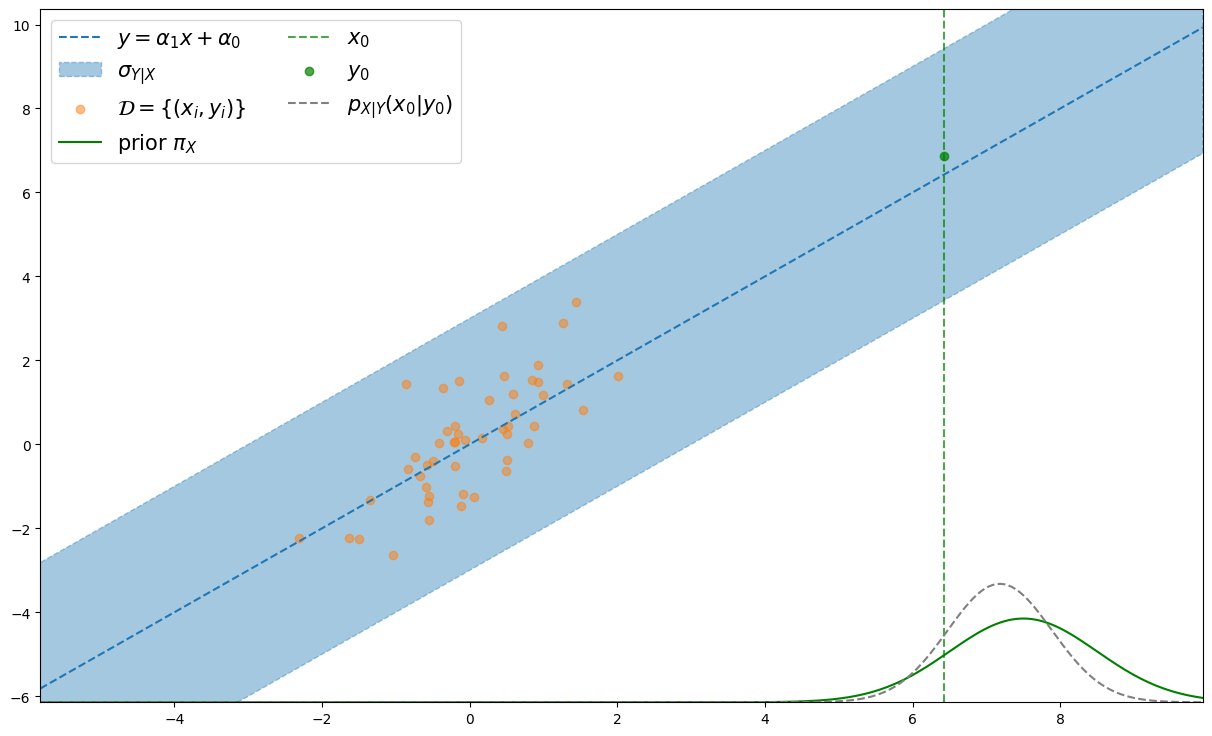
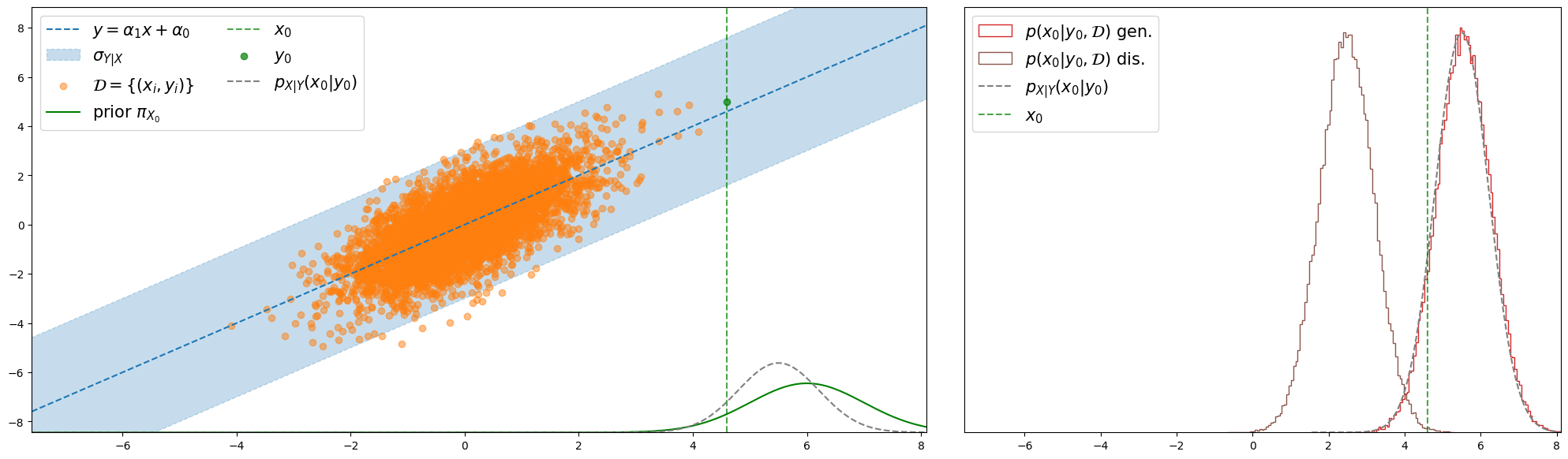
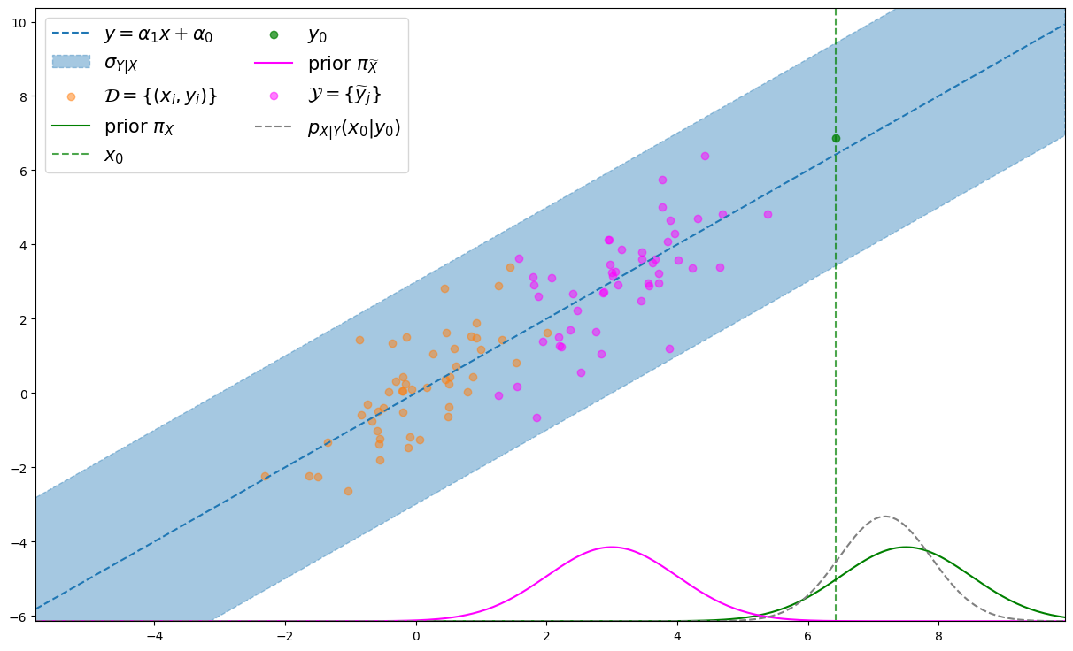
Throughout this paper, we propose to illustrate arguments and conclusions on the continued example of affine regression. Though it serves as an illustrative example, this specific application to affine modeling is, in itself, relevant since affine relationship between variables of interest are most frequent in many science fields and are in many cases, the first considered dependency hypothesis. Let be two real-valued rv (assumed to be) related via an unknown DGP. For illustration purposes, we consider a toy setting where the DGP is of the form:
| (4) |
We dispose of recorded data produced by the DGP, and where the distribution of the values is . The prior knowledge on is given by the distribution . We chose the prior and the DGP to be conjugated such that the posterior distribution reads:
| (5) |
and so this posterior distribution can be used to assess the quality of the inference when comparing the ppd to it; but we otherwise suppose the DGP unavailable. An example of this setting is illustrated in figure 1.
2.1 Generative versus Discriminative modeling
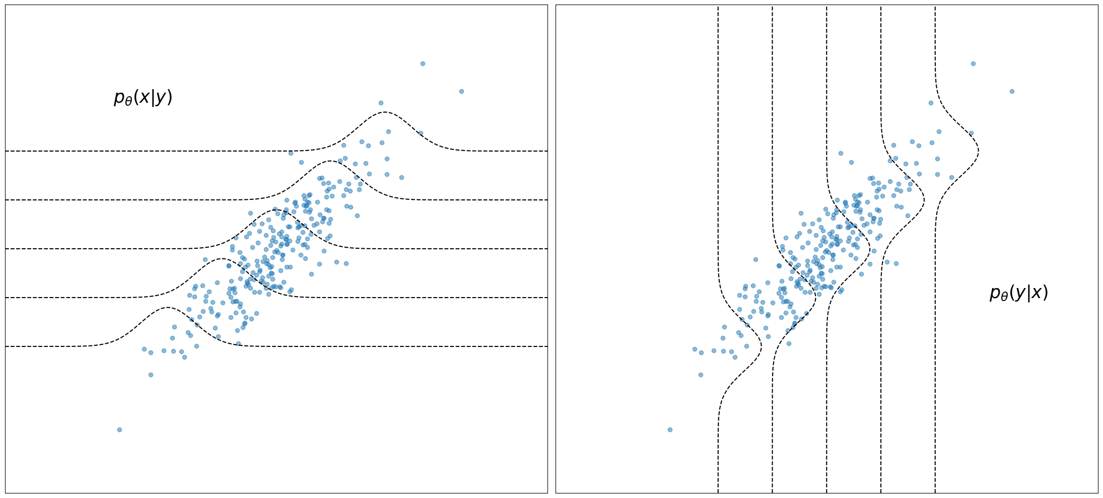
In the previous section we explained the general principle of modeling the posterior pdf (1), and we emphasized on the role of the ppd (2), which accounts for the epistemic modeling uncertainty. However, we have not explained precisely yet how the modeling is carried out. In fact, using a parametric conditional probability distribution , we can either model the unknown DGP with and deduce the corresponding posterior via the Bayes formula, or model the posterior directly with . In the literature, the first approach is classically referred to as Generative (since it models the data generating process), while the second one is called Discriminative (since it makes sense in particular in the classification setting, where the model directly computes the label probabilities which enable to discriminate samples via their respective classes). The first approach is called generative modeling but in the (deep) Machine Learning literature, generative modeling [8] can also refer to the task building a parametric probability distribution which is generative in the sense that it can be sampled from easily and is designed to resemble a probability which produced recorded data. In this paper and unless stated otherwise, generative modeling refers to the approach which consists in building an approximate of the posterior distribution of interest (1) via modeling the unknown likelihood. These two approaches differ in their philosophy: the first one models only what is unknown, i.e. the generative process, while the second one directly models the function of interest, i.e. the posterior pdf. Figure 2 provides with an illustration of the difference between the two approaches.
These approaches yield two different equations:
| (6) | |||
| (7) |
in which superscripts and respectively stand for generative and discriminative; this notation will be used throughout the rest of this paper. In both equations, , be it in the generative case or in the discriminative case, is the conditional pdf associated with , and is what is effectively computed with model associated with parameter .
Figure 3 displays a graphical representation of both models and explains how the modeling choice affects the dependence between all the rv. We build upon these two figures by writing the full joint pdf of all rv.
This comparison of graphical models allow us to deduce the joint distribution of all the rv of interest:
| (8) | |||
| (9) |
The difference between generative and discriminative modeling has already been established in the literature. In the context of classification, [56] compares the Naive Bayes Classifier (which is a generative model) and logistic regression (which is discriminative) in term of (asymptotic) classification error and conclude in favor of the generative approach when working with a small amount of training data.
Illustrative running example
We now illustrate the difference between both modeling approaches by performing homoskedastic affine regression with unknown variance Gaussian Noise where model parameters are the coefficients of the affine transform as well as the variance of the unknown noise so . Both the DGP (4) and the posterior (5) belong to the considered parametric family of conditional probability, so both modeling approaches correspond to a well-specified inference problem. We first describe the generative approach . Once again, thanks to the conjugacy of the prior and the previous , the posterior pdf admits a closed-form expression:
| (10) |
We now describe the discriminative modeling approach with the same parameterized :
| (11) |
2.2 Handling multiple observations
The bayesian philosophy behind equation (1) is to assume (i) prior knowledge on (before observation) in the form of a prior and (ii) an observation model. This observation model is assumed to produce from but it might not necessarily be true in practice. In this case, we say that the observation model is mispecified w.r.t. the observation. In our case, we considered the observation model to be the DGP , so (1) is a well specified Bayesian setting. Then, after observing (one or) several observations: . We deduce the posterior pdf:
| (12) |
We often describe this equation as a form of Bayesian updating: we update the prior knowledge with the observations. In section 3.4, we will discuss the role of the prior with regard to both modeling approaches; but in this section, we first specifically examine whether or not each approach enables to easily handle multiple observations in the inference of .
Equations (6) and (7) explain how we can predict the value of from a unique observed value of using model for respectively the generative and the discriminative approach. In this case, both approaches enable computation of the posterior as both equations are tractable (at least up to a constant). By contrast, when we observe not only a single observation but rather a collection of observations from the DGP which originate from the same unknown value of interest, as in (12), then the generative approach allows to handle this situation with a tractable equivalent of (6), while the discriminative one does not.
Indeed, under a generative modeling, we can easily rewrite equation (6) as:
| (13) |
and this formula can be computed up to its constant denominator (w.r.t. ). On the other hand, with a discriminative modeling, equation (7) becomes:
| (14) |
However, factor is always intractable since given by (1) is defined implicitely by the unknown DGP. Therefore, (14) cannot be evaluated, not even up to a constant, when . Finally, only the generative approach allows to conveniently deal with multiple observations. In order to carry on with the comparison of both approaches, we only consider the case of a unique observation , but, concerning the generative modeling, the equations of the rest of this paper still hold with multiple observations.
3 Supervised Epistemic Uncertainty via the ppd
We now discuss how the epistemic uncertainty is accounted for in each approach, be it generative or discriminative. To that end we analyze how the modeling choice impacts the ppd and more precisely how it can be sampled from. We proceed in three steps: first we analyze the model posterior distribution (see §3.1), we then deduce the joint distribution (see §3.2) and we finally come to its (other) marginal of interest, i.e. the ppd (2) (see §3.3).
3.1 model posterior: or
In this section we look at the posterior distribution over model given the observation and the recorded dataset . Using Bayes rule, it can be written as:
| (15) |
It is important to note here that in the previous equation we can cancel out since for any variables involved in figure 3, we have . By glancing at these two equations, we can already see that the probable values of under this posterior correspond to models for which the elements of , the couples , are likely. In this section, we discuss the impact of on this distribution and conclude on whether or not this observation carries information for inference of depending on the modeling approach. To that hand, we start by leveraging equations (8) and (9) to deduce:
| (16) | |||
| (17) |
On the one hand, with a generative approach, indeed depends on , so indeed carries information for inferring of since the two rv are not independent. We can moreover analyze how the information is carried by to a posteriori models. Probable generative models under posterior produce, with high probability, the value for unknown values distributed under the prior . The posterior distribution of models therefore effectively depends on . We finally conclude that the role of in the ppd inference is twofold: (i) in conjonction to the prior it indeed carries information to probable (epistemic) models and (ii) it carries information to probable (aleatoric) values via posterior models .
On the other hand, under a discriminative approach, factors and reduce to (see (17)) so and are independent rv and finally the posterior over reduces to . Let us analyze why observation does not carry any information to a posteriori models. The information carried by to a discriminative model is that it should produce, with high probability, unknown values for . However, this is nothing but saying that is a probability distribution, which we already know by construction of a discriminative model using a conditional probability distribution. So, by contrast with the generative approach, in the discriminative approach, the role of is solely aleatoric, i.e. to infer via probable discriminative models which do not depend on .
3.2 Joint pdf
We now derive the joint pdf given by equation (3) for both generative and discriminative modeling approaches. In the generative case (6), as explained before, the first factor in the joint pdf is . In general, this expression can only be computed up to a normalizing constant since might be intractable. However, this denominator is a constant w.r.t. but it indeed depends on so it must not be treated as a constant in the joint pdf; so, with regard to the joint pdf, the first factor cannot be computed. Moreover, the second factor is , and as we have explained before in the previous section 3.1 indeed depends on . For the same reason, is intractablethe second factor in the joint pdf cannot be computed, not even up to a constant, either. Conveniently, both factors are intractable because of the same factor which appears in the denominator of the first and in the numerator of the second. So, even though none of the two factors can be computed individually, the intractable terms cancel out by multiplication and the joint pdf can be computed up to a constant (w.r.t. both and ) as:
| (18) | ||||
| (19) |
In the discriminative setting, the first factor in the joint pdf (3) reads (see again equation (7)). This quantity is directly computed in a normalized way by model . Moreover, as we pointed out in the previous section 3.1, the second factor reduces to which can be computed up to a constant. So, unlike in the generative case, both factors can be computed and the joint pdf therefore reads:
| (20) | ||||
| (21) |
So in both modeling cases, the joint pdf can be computed (at least up to a constant).
3.3 The ppd
Recall that the ppd (2) is obtained by marginalizing out the rv in the joint distribution (3). The consequence is twofold: first its pdf is obtained by integrating the joint pdf w.r.t. variable ; and second, sampling from the joint distribution provides samples which are distributed under the ppd. In this section, we discuss the first point.
By integrating (18) and (20) w.r.t. , we obtain expressions for the ppd (2) in both cases:
| (22) | ||||
| (23) |
In practice, these two equations can only be used when exact computation of the integral is feasible. Nonetheless, they remain relevant as we can analyze them both to grasp a difference between the two approaches which provides with another interpretation of the ppd. The first formula, in the generative case, corresponds to Bayesian inference using the prior and the marginal likelihood ; while the second formula, in the discriminative case, corresponds to an averaging of posterior predictions. So, in both cases, the ppd is an averaging of the quantity (which is what is effectively computed with model ) w.r.t. . This is to be contrasted with the original definition of the ppd, defined as the average of predictions w.r.t. . These two definitions only coincide in the discriminative case since the model computes directly the prediction (see (7)) and the posterior distribution reduces to (see section 3.1). As a consequence, this means that is an exact construction of the ppd only in the discriminative case.
3.4 Explicit or Implicit prior
A main difference between the two approaches lies in the role of the marginal in the joint pdf . This distribution is of particular interest as it can be considered as a prior in the ppd which is the object of interest in both modeling approach:
| (24) |
We can again leverage both equations (8) and (9) to deduce:
| (25) | |||
| (26) |
These two equations allow to understand that the marginal does not play the same role in the generative and discriminative cases. While in the former setting this immutable marginal distribution describes prior knowledge and does not depend on (see equation (25)); in the latter setting, this marginal distribution is the result of an intricate interaction between the dataset , the prior distribution and the DGP . On the one hand, in the generative approach, it corresponds to the prior which can be specified according to the problem at hand and, in itself, may provide significant information about the value of interest . In practice, this prior distribution can also play a role of regularization and may as well be understood as a safeguard since it can effectively constrain the prediction to a specific region of the space [76][71][64] but more importantly, the prior distribution is often the result of an elicitation effort [67] which consists in of (i) obtaining prior information and (ii) transcribing this knowledge into a probability distribution. On the other hand with a discriminative approach, this marginal has a very different role. The relevance of equation (26) first lie in the fact that it highlights the systematic intractablity of pdf . Indeed, it can never be computed (even if exact integration was feasible) since it ultimately involves computing the pdf in , which is unknown by assumption. This intractability does not pose any practical issue since the computation of the marginal (26) is not required for computing the joint pdf (20) (and consequently not for computing the pdf of (or sampling from) the ppd). But this also means that the discriminative construction does not allow to leverage any information encapsulated in, or any practical property induced by, a prior distribution during the inference. We now rewrite the expression of equation (26) as:
| (27) |
So, this distribution has a pdf which indeed depends on (i) via the unknown and is indirectly related to (ii) the prior and (iii) the DGP via . As a consequence, this distribution will attribute high probability mass to the values which have high probability under for some value . As such, an implicit density estimation mechanism of shifts the distribution away from and towards the regions of high probability under . This implicit density estimation mechanism appears clearly in the limiting case where the aleatoric uncertainty increases since we observe that pdf becomes . Conversely, when the aleatoric uncertainty decreases, this pdf is, under assumptions of identifibility and invertibility, . We will illustrate this effect in both contexts of regression (using the running example) and classification. As a consequence, the ppd in the discriminative approach indeed does not provide with an approximation of (1) with prior . It instead provides with an approximation of:
| (28) |
Consequently, a mismatch between the prior and the distribution , which effectively generated the values in , will result in a mismatch between the target posterior (1) and the ppd (2). Subsequently, only the regions of space which are well represented by the values in dataset will have high probability mass under the marginal , and hence, under the ppd . Though this argument relates to the posterior (via the distribution ), we consider that this argument is not related to epistemic uncertainty as (i) the effect does not vanish when the number of recorded observation, i.e. the size of increases; and (ii) the same effect can be observed when considering where is a unique parameter (such as MLE or MAP) estimate.
Finally, in the discriminative case, it is of particular interest to study the distribution as it corresponds to the average prediction over observations since .
This, together with the probability mass of which favors the regions of values in , tells us that a discriminative model will favor the regions which are well represented in the dataset. In a classification task, the dominant labels will be predicted more often than the others, thus explaining that discriminative models indeed suffer from imbalanced dataset. We further emphasize this precise point using the illustrative running example, a classification example provided in supplementary materials (see section
3.4.1),
as well as in quantitative simulations in section 5.
Illustrative running example
We now leverage the affine regression example to illustrate the effects of the implicit prior on the ppd in the discriminative modeling approach. We first display an empirical approximation of the distribution . To that end, using equation (27), we obtain samples from this distribution via the two step sampling procedure and (the second sampling step is detailed in the next paragraph 3.5). Of course in practice, the first sampling step cannot be conducted as sampling from requires sampling from the DGP which we recall is unknown by hypothesis, but in our example, we do resort to this sampling procedure for illustration purposes.
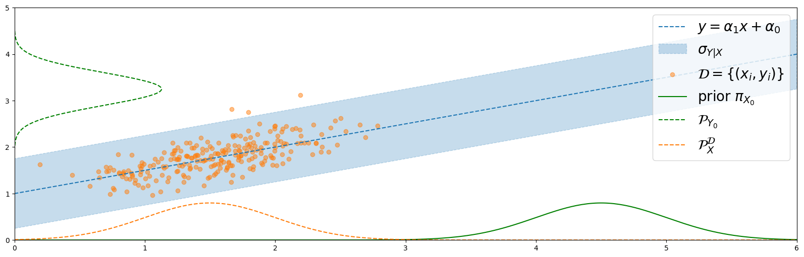
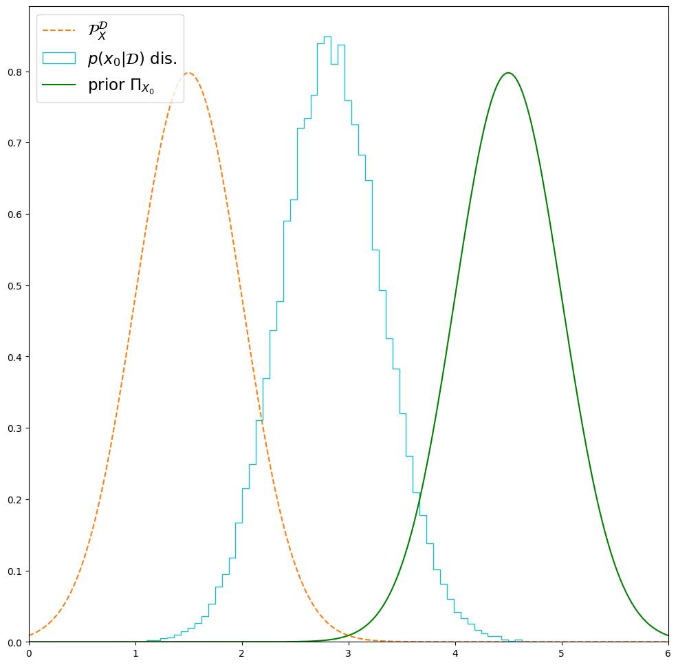
In figure 4, an empirical estimate of is obtained via the described two-step sampling procedure (upper-left and lower-left) and is plotted against prior and . We see that, in the discriminative setting, (which we recall acts as a prior in (24)) indeed corresponds to a trade-off between the two distributions and is shifted towards via an implicit density estimation mechanism from the -values in . In this example, we can also visualize how the DGP affects the balance between and which we now illustrate in the next figure 5.
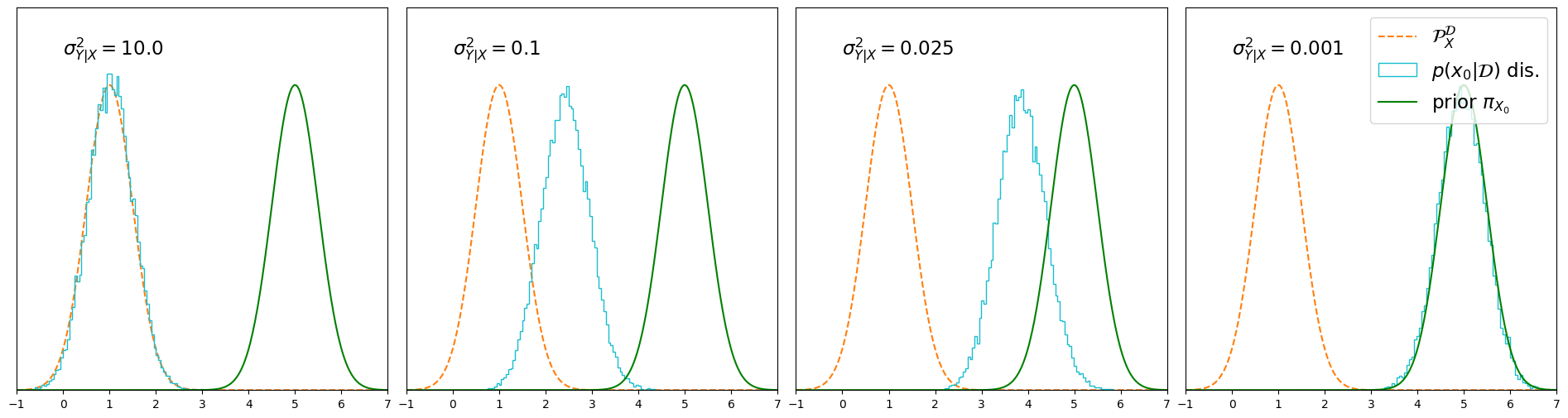
In this figure, on the one hand, we see that for lower values of (the noise standard deviation in the DGP (4)) the distribution gets closer to ; while, on the other hand, this distribution gets closer to for larger values of . This example seems to hint that when the DGP is stained with high (resp. low) aleatoric uncertainty, the distribution leans more towards (resp. ). In section 3.4.1, we provide with another example of classification and observe a similar effect.
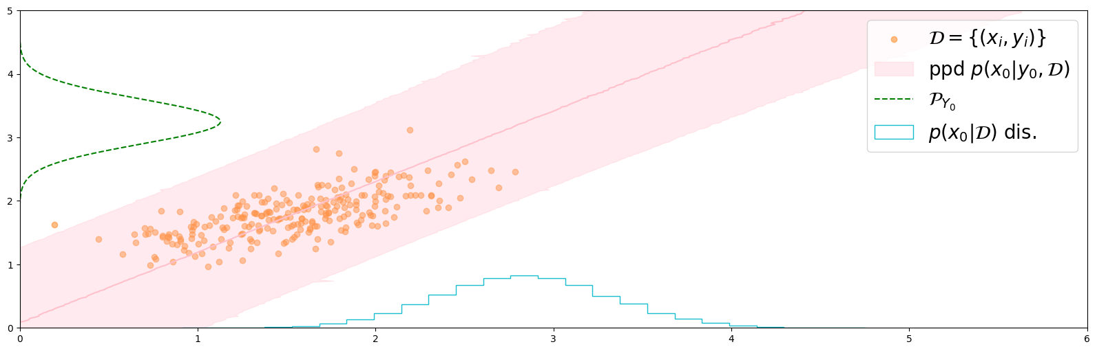
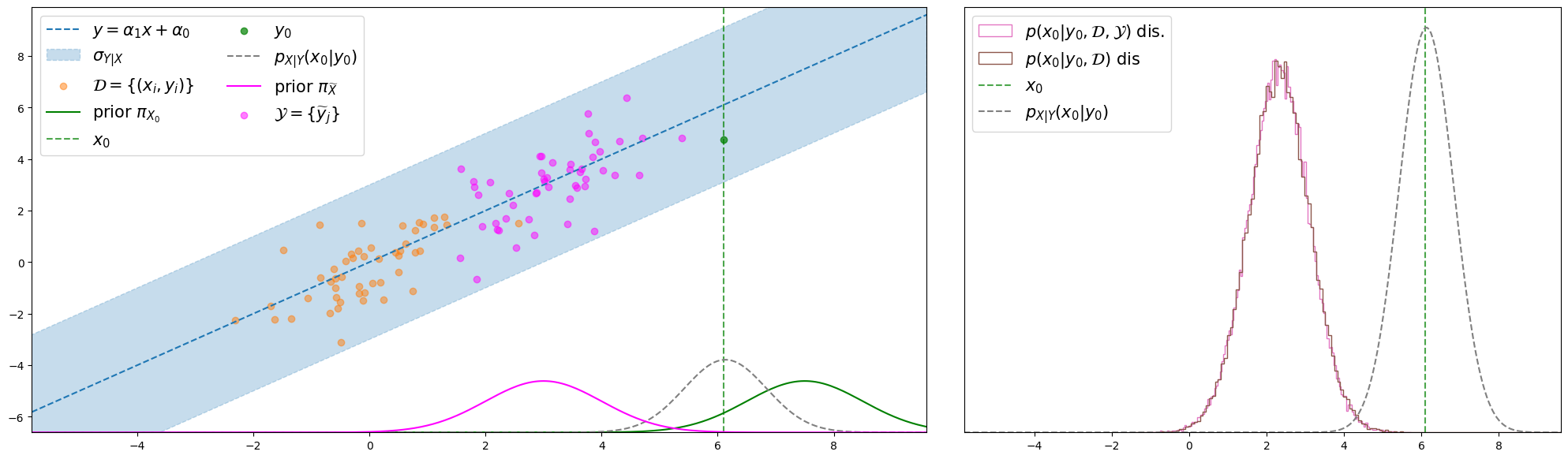
As we have mentionned before, it therefore follows that the ppd in the discriminative case provides with an approximation of (28), which leads to a visible mismatch between the ppd and the true (unknown) posterior when the prior and are different probability distributions, which we now illustrate. To that end, we compare this pdf to an histogram of samples from the ppd with large to remove the effect of epistemic uncertainty and we observe that they perfectly match. Conversely, when the prior and are the same probability distribution then the ppd indeed approximates the true ppd. This is illustrated in figure 6.
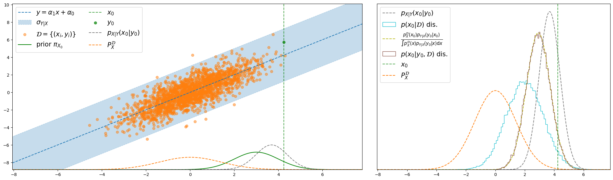
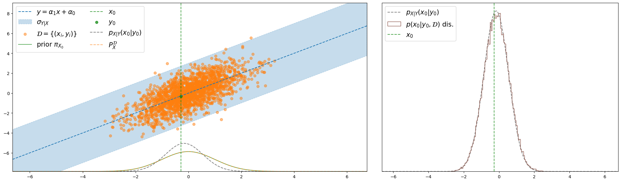
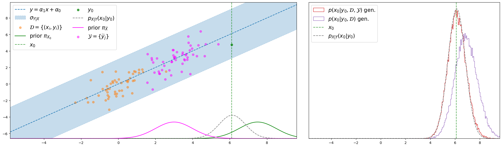
We now illustrate a more problematic issue related to the same mechanism. Because the dataset shifts the distribution , which acts as a prior in the ppd, toward via an implicit density estimation mechanism of with the ppd will only assign high probability to the regions of space which are assigned high probability under . The consequence of this in the case of affine modeling is that we are not able to predict accurately outside of the support induced by as the ppd attributes little to no mass to the true value of . A discriminative affine model cannot extrapolate to regions outside of the support of and this conclusion argues, for once, in disfavor of a discriminative approach since an affine model, amongst all models, is expected to extrapolate well. Conversely, as a result of the explicit prior, the generative approach does not suffer from the same shortcoming and we observe that the affine generative model indeed produces a ppd which assigns high probability to the true value of and approximates the true unknown posterior. This is illustrated in figure 7.
3.4.1 Classification example
In the previous example of regression, we illustrated how a discriminative modeling approach builds an implicit prior via a density estimation mechanism, resulting in a poor approximation in the case of a mismatch between and the desired prior . We also illustrated how, in a discriminative model, the dataset , the prior and the DGP interact to yield which, via an implicit density estimation mechanism, is a trade-off between and . We now also illustrate this specific effect on a classification problem where is a Categorical variable taking value .
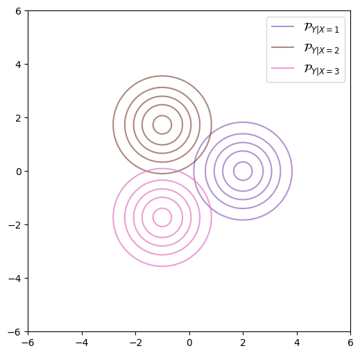
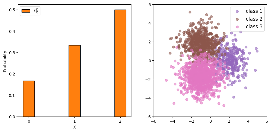
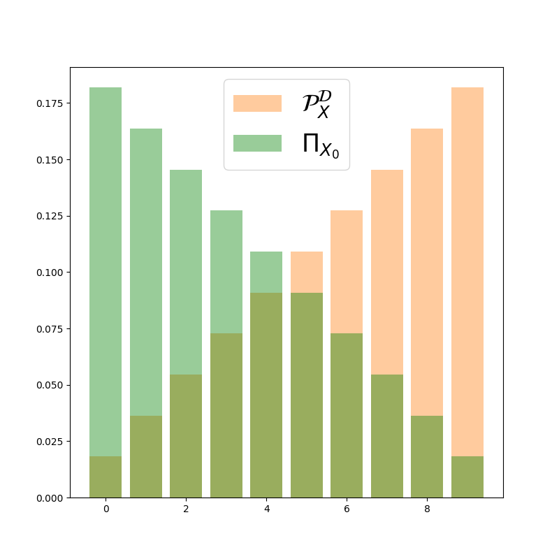
We consider a 2-dimensional example with where the DGP reads: with . In this DGP, the aleatoric uncertainty can be controlled via the value of which describes the distance of each Gaussian class to the origin ( stands for radius). Indeed, the further the different classes are from each other, the easier it is to accurately classify a sample to its according unknown label. The goal of this section is to illustrate the effect of the roles of distributions and in the discriminative approach. We therefore select the two distributions from be different to one another: for versus for for labels . The distribution defines the frequencies of classes, and together with the DGP can produce a toy dataset which is illustrated in the next figure 9.
As a discriminative model, we use a multinomial Logistic classifier which class probability reads:
| (29) |
where with . Similarly to the continued regression example, we will display an empirical estimate of distribution (26) obtained by the sampling procedure: (via the unknown DGP which we use only for illustrative purposes), and given by equation (29).
A prior distribution over parameters which would be conjugate to this logistic model would lead to a posterior available in close form, but unfortunately, such a conjugate prior does not exists amongst the usual probability distributions. We therefore use a simple Gaussian prior over parameter and resort to sampling from the ppd using an Metropolis-Hastings MCMC algorithm, though a Gibbs sampling scheme is also available in this setting [34]. In the next figure, we display empirical estimates of against and .
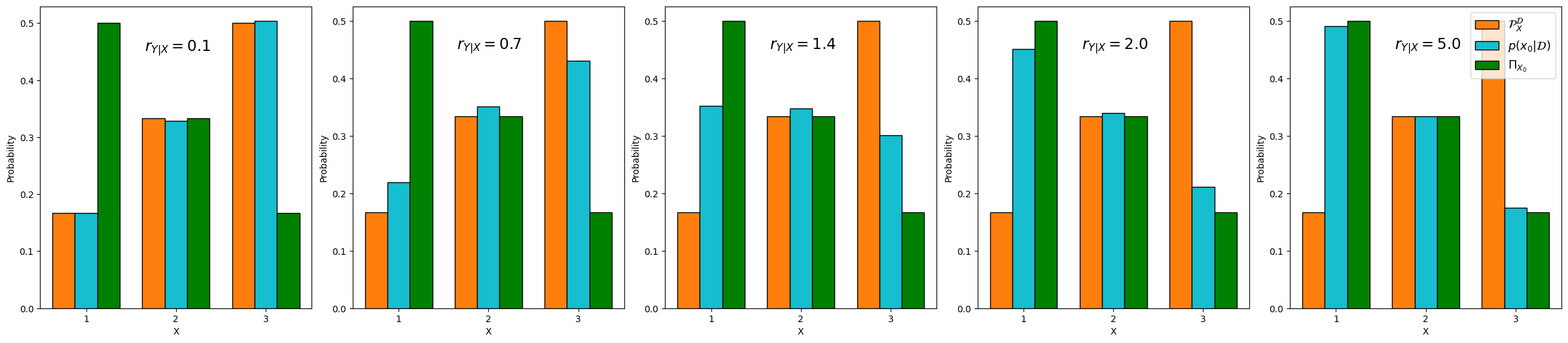
This figure once again illustrates that distribution (which we recall acts as a prior in the ppd (24)) corresponds to a trade-off between and . With a very similar interpretation to that of figure 5, this figure also seems to hint that the dynamic of the DGP dictates the trade-off between the two distributions: high (resp. low) aleatoric uncertainty shifts more towards (resp. ).
3.5 Gibbs sampling from the ppd
We now come to sampling from the ppd. Samples from the ppd can be obtained in two distinct ways. If exact computation of expectation w.r.t. is feasible, then (22) and (23) give tractable expressions (possibly up to a constant) for the ppd. However, the integrals in these equations admit closed form expressions only in specific cases when using conjugate models, and exact integration is, more often than not, unfeasible making the posterior pdf intractable. So in practice, we rather resort to sampling via the joint distribution since, as we explained before, sampling from the joint distribution (3) produce samples that are distributed according to the ppd (2).
With that regard, in both modeling cases, the joint pdf, (18) and (20), can be computed (at least up to a constant), and so we can sample from the joint distribution via the pdf. More conveniently, the discriminative approach yields a specific factorization of its joint pdf (20) which enables a sequential sampling procedure with and . It is therefore motivated to construct models for which the posterior probability distribution of parameters By contrast, the generative approach does not induce the same factorization and does not benefit from the same convenient sequential sampling scheme. In this section, we propose a general scheme for sampling from the ppd which can be applied to both modeling approach.
We now propose a scheme that enables to sample from the joint distribution (3), and therefore from its marginal which is nothing but the ppd (2). This sampling scheme is based on the notorious Gibbs sampling [10][24] which is an MCMC algorithm [68] that applies specifically to a joint distribution with a markov transition . This transition leaves the joint distribution invariant since the Gibbs algorithm can be seen as two steps of Metropolis Hastings [12] transition where the acceptance probability is . We apply the principle of Gibbs sampling to the joint distribution in the generative (resp. discriminative) setting. First, conditionally on the current model , is distributed according to the posterior for that model. So the first step of the markov transition is to draw from equation (6) (resp. (7)) with . Then, conditionally on the current value of , is distributed according to and so the second step of the markov transition consists in sampling with the analogous of (19) (resp. (21)) where . We summarize this Gibbs sampler in algorithm 1 (for the moment readers should disregard the red parts of the algorithm, as they are related to the semi-supervised learning task covered in section 4).
Though this algorithm is written in a similar fashion in both modeling approaches, the conclusions with regard to the different behaviours of the two modeling approaches presented in the previous sections still hold as they are the result of a structural difference between the generative and discriminative approach. This algorithm will be especially useful in the semi-supervised setting, which we describe in the next section 4.
In the case of multiple observations as in section 2.2, the previous algorithm can be effortlessly adjusted in the generative case (recall that the discriminative case is not compatible with multiple observations, see section 2.2). Indeed in this setting, at time , we first sample according to (13) for current model ; and then the dataset is augmented into .
Illustrative running example
We now come back to the continued example of affine modeling to provide an example of the Gibbs algorithm mechanism. We assume prior knowledge over parameter in the form of where and is a covariance matrix, is the pdf associated with an inverse Gamma distribution and are respectively the shape and scale parameters of the corresponding Gamma distribution. Unfortunately, the posterior does not admit a closed form expression; but, at least, this choice of conjugate priors allows for both conditionals to be tractable. We first explicit these two conditionals pdf in the generative (resp. discriminative) setting:
| (30) | |||
| (31) |
| (32) | |||
| (33) |
So in both modeling cases, the posterior distribution can be sampled from using a Gibbs scheme by sequentially sampling these two conditionnals. Then, from a Gibbs sampling of affine models, we can almost effortlessly obtain samples from the ppd by including the additional step of sampling from for the current model parameters within the Gibbs sequential Markovian transition. Again, in supplementary material, we summarize this Gibbs sampler in the specific case of affine homoskedastic modelling, see algorithm 2 (readers should disegard the steps in red for now, as they are related to semi-supervised learning which we now discuss).
4 Bayesian Semi-Supervised learning
In this section, we now build upon the equations, arguments and conclusions presented in the previous sections to tackle the problem of semi-supervised learning. As we have mentionned before, supervised learning techniques use the observed variables and their corresponding labels to build a model which capture the dependency between two rv and which can be used to make predictions about the label conditionally on the value of observed rv. Conversely, unsupervised learning [33][31] take interest in learning pattern in a data distribution without considering the notion of associated labels. Structure can be represented by data clusters obtained by K-means [46][45], graph-based clustering methods such as spectral clustering [57] or Louvain method [7], or via maximum-likelihood in a mixture probability distribution model [15]. In the beginning of this paper, we explained that the Generative approach for modeling the unknown posterior, should not be confused with the tasks and techniques of Generative modeling. These techniques can also be considered as unsupervised learning as they enable to capture the structure from univariate data such that the corresponding probabilistic model can be sampled from easily in order to obtain observations which are approximately distributed according to the dataset distribution. Most popular methods include Variational AutoEncoders [40], Generative Adversarial Networks [27], Normalizing Flows [60] and Diffusion models [70] but this is beyond the scope of this paper. Semi-supervised learning does however lie within the scope of this paper as it aims to obtain a conditional model to predict label from observations, but the goal is to infer the model from both a labeled dataset and unlabeled observations. In this section we now build upon the previous arguments and discuss the compatibility of both learning approach with this learning task.
4.1 The learning task
In section 2 and onward, we presented the general task of learning a model for the posterior (1) using a set of labeled observations , and how to predict about an given a corresponding observation with the ppd, which we now refer to as a supervised learning task. However, in many statistical learning settings, we also dispose of unlabeled observations. They corresponds to values , which we know (or assume) are produced by the DGP, but for an unknown values for which we assume prior knowledge : . When the observations in and cover different regions of the observation space, and/or when has a significant amount of elements, then the unlabeled observations may contain significant or non-negligible information [58]. In this context, a semi-supervised learning task aims at inferring a model from both labeled and unlabeled observations. This question has risen in importance in importance where we dispose of a lot of unlabeled observations, but where the labelling tasks is expensive (as it is the case when the labelling needs to be conducted by a human operator).
The ppd (2) then becomes:
| (34) |
and we aim to compute this pdf, or sample this distribution if exact computation of the integral is not feasible. This formulation is more general than the one described in section 2 and it reduces to supervised learning in the case where .
Throughout this section, we will carry on using the continued example of affine modeling to illustrate the arguments and conclusions. To that end, we suppose that, in addition to , we also dispose of unlabeled observations produced from the DGP (4) via an unknown label for which we suppose prior knowledge in the form of a prior which is supposed to be the same for all and which we consider to be Gaussian . The semi-supervised setting is illustrated in figure 11.
4.2 Both modeling confronted to the semi-supervised learning task
We now confront the two modeling approaches to the specific problem of semi-supervised learning by analysing the model posterior which reads:
| (35) |
We first explain that the discriminative approach does not allow for Bayesian semi-supervised learning. To see this, recall the conclusion of section 3.1: when we do not know , the posterior over does not depend on and so this observation does not carry any information to the discriminative models. Therefore, the same applies for the elements of : since we do not know the label , the unlabeled observation does not bring any information on as the posterior over models does not depend on . Finally, the model posterior (35) reduces to , (34) reduces to (23) and all the other equations in section concerning the discriminative modeling approach remain unchanged.
Conversely, the generative approach indeed allows for semi-supervised learning. In section 3.1, we explained that, even though we do not know the value of , the posterior distribution over models still depends on the observation indirectly through the prior . With a similar argument, we understand that the unlabeled data indeed carry information on model . We write: . So, even though we do not know the label , probable generative models under (35) produce, with high probability, the value of for some unknown label distributed under the prior . In a classification setting, this term can indeed be computed as a tractable finite sum [4][37], but in general, this term is only available in integral form making the joint pdf , intractable, not even up to a constant. This raises the question of sampling from the ppd since its pdf is intractable. In the next section, we propose to use a variation of the Gibbs algorithm presented in section 3.5, and which allows to sample from this ppd.
4.3 A Gibbs sampling algorithm for semi-supervised learning
In this section we extend the previous Gibbs sampling algorithm presented in section 3.5 for sampling from the ppd (34) in the case of generative semi-supervised learning. To that end, we apply the Gibbs mechanism of sequentially sampling the conditional distributions in the joint distribution . Firstly, conditionally on the current value of , the labels are independent and each distributed according to its own posterior distribution. So the first step of the Gibbs markovian transition is to sample with equation (6) (as in section 3.5) and . Secondly, conditionally on the current label values , the model parameters are distributed according to . So the second step of the Gibbs markovian transition is to sample analogous of equation (19) where . We summarize this Gibbs mechanism in algorithm 1 and we highlight in red the steps which are effectively responsible for semi-supervised learning.
In the case of semi-supervised learning setting, this Gibbs algorithm is all the more crucial. Indeed, while in the supervised context the Gibbs approach was only an alternative option to sampling from the joint distribution which pdf (18) could be computed up to a constant; in the case of semi-supervised learning however, it is possible that this joint pdf cannot be evaluated, not even up to a constant and the Gibbs approach is therefore very convenient for sampling the corresponding ppd.
We have written the Gibbs algorithm with including to perform semi-supervised learning for both modeling approach but of course, as we have mentionned before, the semi-supervised ppd (34) reduces to the supervised ppd (2) in the discriminative setting, so this Gibbs algorithm, even though it involves , is not able to leverage any information from the unlabeled observations in this modeling approach. We therefore would like to stress that the semi-supervised learning is not enabled by the Gibbs procedure itself but rather by using a generative modeling instead of a discriminative one which induces different conditional dependency between all the rv. We proposed the Gibbs algorithm as a way to sample the joint distributions in the case of generative modeling (with possibly in the supervised setting) which is particularly convenient to use because of the conditional independence (w.r.t. ) of labels . However, this Gibbs scheme it is only a possible approach for sampling from the corresponding ppd which effectively depends on .
We now come back to the continued example of affine modeling and use it to illustrate the practical use of the Gibbs sampling algorithm which we use to illustrate, respectively, the compatibility and incompatibility between the generative and discriminative approaches and the semi-supervised learning. In algorithm SM3.1 we first explicit how to build upon the supervised Gibbs sampling algorithm of the supervised ppd presented in section 3.5 to obtain a Gibbs sampling scheme of the semi-supervised ppd.
In this case, the generative and discriminative approach yield two different equations for the posterior :
| (36) | |||
| (37) |
The Gibbs sampling procedure for semi-supervised learning of affine homoskedastic is summarized in algorithm 2. Again, the steps highlighted in red are indeed responsible for leveraging information from the unlabeled observations.
We will now illustrate whether or not the modeling approach enables leveraging information in to contribute in reducing the epistemic uncertainty. We first provide empirical evidence that the discriminative approach is unable to leverage information in unlabeled observations to reduce the epistemic uncertainty. To that end, we consider a setting where contains few points leading to high epistemic uncertainty to be reduced; and we apply the previous Gibbs sampling algorithm SM3.1 in the discriminative case with and without unlabeled observations and visually observe that the resulting samples seem to follow the same distribution. This empirical illustration is presented in figure 12.
We further perform a Kolmogorov-Smirnof statistical test where the null hypothesis is the samples obtained from the supervised and semi-supervised Gibbs sampling algorithm are from the same (unknown) distribution. This test works from two set of iid samples; but the samples from the Gibbs sampling algorithm are correlated samples so we first extract (almost) uncorrelated samples sub-sampling the Markov chain at every each integrated auto-correlation time steps. The Kolmogorov-Smirnof test yields a -value of and we cannot reject the null hypothesis with low error probability; which indicates that the data i.e. the two sets of de-correlated samples is consistent with the null hypothesis i.e. that they originate from the same underlying probability distribution.
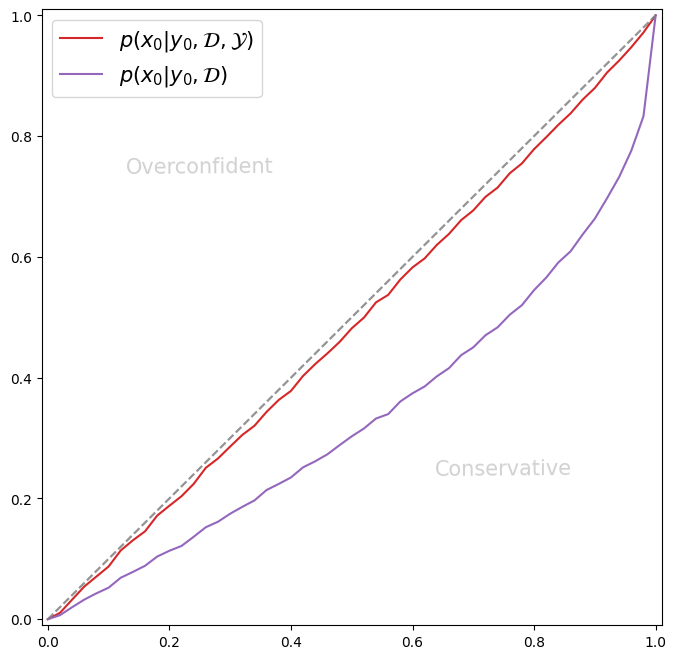
Conversely, in the generative modeling approach, we go back to the setting presented in the previous figure 11, and we compare the supervised and semi-supervised ppds, from which we obtain samples via the corresponding Gibbs sampling algorithm 2 with and without . The results are presented in the next figure 13(a). We compare the empirical distributions (built an histogram of the samples) and we visually observe that the semi-supervised ppd provides with a better of the true unknown posterior than the supervised ppd. To go further than a visual interpretation, we compare the calibration curves of the both ppds. The calibration curve allows to assess the quality of an approximation and is computed from the pdf of the target posterior, in our case the true unknown posterior and from samples from the approximating distribution, in our case the (supervised or semi-supervised) ppds. It is built by computing, for values , the -highest density region of the target distribution using the pdf and computing the proportion of samples which land in that region. We can therefore conclude that the unlabeled observation were taken into account during the inference and indeed contributed to reducing the epistemic uncertainty.
4.4 Parallel inference
In this section we propose to re-discuss the problems of supervised and semi-supervised learning by considering them as solving two (or several) posterior inferences at the same time. To that end, we now denote the set of unknown labels associated to the unlabeled observations. On the one hand, are not necessarily label values of interest in the initial problem (that of inferring via ), it is nonetheless an unknown rv related to via the same unknown DGP and can be associated to an inference problem (again, possibly irrelevant in the context of the initial problem). On the other hand, both and can be values of interest. Indeed, in many learning instances, we dispose of a training dataset (the set in our paper) to infer the probable models; and given another set of observations (the so-called testing dataset), our aim is to predict for each of them the associated label (which is different from one observation to another, as opposed to section 2.2, where one common label produced several observations). In this case, all the observations in the testing dataset play an epistemic role in the generative case. More precisely, the observations of the testing dataset act as unlabeled observations resulting in an underlying semi-supervised learning setting. This is illustrated via quantitative simulations in the next section 5.
In this context, since we are trying to infer from and from via probable models using the same observations , the two inference should not be treated as independent problems in both modelling approaches. However, a main difference between the two modeling approaches can be understood when considering two (or several) inference problems at once.
In the discriminative setting, we have that so the inference of (resp ) does not depend on (resp ). As such, each inference problem can be solved via sampling from its corresponding ppd. Conversely, in the generative setting, all the observations act as unlabelled observations in both inferences and the two problems should not be treated independently as all the unlabeled observations contribute to reducing the epistemic uncertainty. As a result, and both inference can not be solved by sampling from each corresponding ppd, and this modelling approach instead calls for a sampling from the joint distribution. Finally, note that the previous semi-supervised algorithm, which we proposed as a way to obtain samples from the posterior was constructed by applying the Gibbs sequential sampling mechanism to the joint distribution and as such, produced desired samples from but also, as a byproduct, samples from , effectively solving both inference problems at once. Again of course, since the Gibbs is only a tool for solving the inference problem, the underlying structure of dependency between rv is preserved. So in the discriminative case these distributions respectively reduce to and .
5 Simulations
Throughout the paper, we leveraged the example of affine homoskedastic modeling in the case of univariate regression to illustrate the arguments of this paper. As we mentionned before, this illustrating example can be relevant to some readers as modeling affine dependencies is a most frequent problem in many scientific fields. We also used this example as it enables, with appropriate choice of priors, to run a straightforward Gibbs sampler for both the generative and discriminative modeling approaches. However, considering models which enable such convenient sampling procedures with closed-form (or all its conditionals in a Gibbs scheme) indeed heavily restricts the choice of model . In this section we now consider conditional models which are defined using NN functions with tractable pdf, but for which we are not able to elicit a prior over parameters such that the posterior distribution admits a closed form expression, and we resort to approximate sampling from that posterior using Stochastic Gradient Langevin Dynamics [72] [19].
In this section, we tackle the problem of classification in which is hence a Categorical rv. We evaluate generative and discriminative models both defined via NN functions (we describe the specific structure hereafter) and with similar number of parameters. We proceed to assess the classification accuracy of a generative versus discriminative model for via Gibbs sampling. We consider three different scenarios which we now describe.
Following the idea described in section 4.4, we now consider two distincts sets: the training dataset , and a testing dataset . All the labels are distributed according to , and in the following we address three scenarios, which differ on the size of the testing set, and the possible discrepancy between and .
Scenario 1: Identical priors and sizes. We first consider the scenario where the label distribution from the training dataset coincides with the prior. So , and as such, couples (which belong to training dataset ) and (which belong to the testing dataset) have the same distributions. This corresponds to the most frequent situation in practice and we use this setting as a baseline. We consider the dataset and the set of unlabeled observations to be of the same size, i.e. .
Scenario 2: Imbalanced dataset (different priors, same sizes). We then consider the scenario where , so couples and do not have the same distributions (and indeed are quite different - see figure 14). We still set .
Scenario 3: Few labeled samples (same priors, different sizes). We finally consider the scenario where , but , so we dispose of a few labeled observations in , and of a large amount of observed values for which we want to infer the corresponding label . In this setting, the low number of observations in will hinder the prediction accuracy of both models, but as we have explained before, the large amount of unlabeled observations act as an unlabeled dataset in the generative case.
We consider both the classification datasets of MNIST and of FashionMNIST, for which we reduce the dimension of observations via a Principal Component Analysis [63] in order to keep of explained variation. We compare a discriminative model which is a fully connected NN with 4 hidden-layers of 256 units to a generative model which is built using a combination of invertible conditional Normalizing Flows layers [17] and stochastic ones [3]. We sample from the joint distribution via Gibbs sampling with steps. The results are provided in the next table 1 and for each dataset and scenario, we consider 10 independent runs and we display the average classification accuracy as well as the standard deviation.
| Dataset | MNIST | FashionMNIST | ||
| Model. | Disc. | Gen. | Disc. | Gen. |
| Scenario 1 | ||||
| Scenario 2 | ||||
| Scenario 3 | ||||
We now analyze the results of this experiment. Comparing the results for the first scenario tells us that the generative modeling can indeed be on par in terms of classification accuracy when compared to its discriminative counterpart. This scenario can be used as a baseline experiment for the two following scenarios. In the second scenario, the distribution of labels in the dataset, , is different from , leading to a situation of imbalanced dataset. In this situation, we notice that the discriminative model indeed suffers in term of accuracy as it favors the dominant classes of the dataset. As we have explained, the generative approach does not suffer from such dataset imbalance, or at least not as much, which is confirmed in this experiment. This is in accordance with the discussion of section 3.4. Finally, in the third scenario, the lower number of labeled observation in hinders, as expected, the classification accuracy of the discriminative model as compared to its generative counterpart, as the latter indeed leverages the unlabeled observations in the inference of probable models, which indeed contributes to reduce the modeling epistemic uncertainty, as discussed in section 4.2.
Conclusion
Throughout this paper, we discussed the epistemic uncertainty quantification in generative and discriminative models, and draw several conclusions. On the one hand, discriminative models are an easy-to-use tool since they can be parameterized easily and directly approximate the posterior. Moreover, if they can be sampled from easily, then one can use a straightforward two step procedure for sampling from the ppd, which indeed enables to quantify the epistemic uncertainty. However, by nature discriminative models do not take into account the information contained in the prior distribution, which is replaced by an implicit prior inferred on the dataset. As a result, they suffer from imbalanced datasets. Finally they cannot be conveniently used in the context of inferring from multiple observations, and they cannot leverage information from unlabeled data.
On the other hand, generative models are perhaps less convenient to use as they usually require a more sophisticated structure and require an additional inference step, in addition to the prior distribution, to sample from the corresponding posterior. Yet by construction they do enable to leverage information from all available sources, making them an appealing tool, in particular in a semi-supervised context. In practice, the two-step procedure for sampling from the ppd is no longer available; but our general purpose Gibbs sampling based algorithm indeed enables to sample from the ppd (and thus perform epistemic uncertainty quantification) while taking into account both the labeled and unlabeled observations.
References
- [1] Alexander C Aitken. On least squares and linear combination of observations. Proceedings of the Royal Society of Edinburgh, 55:42–48, 1936.
- [2] Ahmed Alaa and Mihaela Van Der Schaar. Discriminative jackknife: Quantifying uncertainty in deep learning via higher-order influence functions. In International Conference on Machine Learning, pages 165–174. PMLR, 2020.
- [3] Elouan Argouarc’h, François Desbouvries, Eric Barat, Eiji Kawasaki, and Thomas Dautremer. Discretely indexed flows, 2022.
- [4] Andrei Atanov, Alexandra Volokhova, Arsenii Ashukha, Ivan Sosnovik, and Dmitry Vetrov. Semi-conditional normalizing flows for semi-supervised learning. arXiv preprint arXiv:1905.00505, 2019.
- [5] Atilim Gunes Baydin, Barak A Pearlmutter, Alexey Andreyevich Radul, and Jeffrey Mark Siskind. Automatic differentiation in machine learning: a survey. Journal of machine learning research, 18(153):1–43, 2018.
- [6] Joseph Berkson. Application of the logistic function to bio-assay. Journal of the American statistical association, 39(227):357–365, 1944.
- [7] Vincent D Blondel, Jean-Loup Guillaume, Renaud Lambiotte, and Etienne Lefebvre. Fast unfolding of communities in large networks. Journal of statistical mechanics: theory and experiment, 2008(10):P10008, 2008.
- [8] Sam Bond-Taylor, Adam Leach, Yang Long, and Chris G Willcocks. Deep generative modelling: A comparative review of vaes, gans, normalizing flows, energy-based and autoregressive models. IEEE transactions on pattern analysis and machine intelligence, 2021.
- [9] Léon Bottou, Frank E Curtis, and Jorge Nocedal. Optimization methods for large-scale machine learning. SIAM review, 60(2):223–311, 2018.
- [10] George Casella and Edward I George. Explaining the gibbs sampler. The American Statistician, 46(3):167–174, 1992.
- [11] Changyou Chen, David Carlson, Zhe Gan, Chunyuan Li, and Lawrence Carin. Bridging the gap between stochastic gradient mcmc and stochastic optimization. In Artificial Intelligence and Statistics, pages 1051–1060. PMLR, 2016.
- [12] Siddhartha Chib and Edward Greenberg. Understanding the metropolis-hastings algorithm. The american statistician, 49(4):327–335, 1995.
- [13] Kyle Cranmer, Johann Brehmer, and Gilles Louppe. The frontier of simulation-based inference. Proceedings of the National Academy of Sciences, 117(48):30055–30062, 2020.
- [14] Katalin Csilléry, Michael GB Blum, Oscar E Gaggiotti, and Olivier François. Approximate bayesian computation (abc) in practice. Trends in ecology & evolution, 25(7):410–418, 2010.
- [15] Arthur P Dempster, Nan M Laird, and Donald B Rubin. Maximum likelihood from incomplete data via the em algorithm. Journal of the royal statistical society: series B (methodological), 39(1):1–22, 1977.
- [16] Armen Der Kiureghian and Ove Ditlevsen. Aleatory or epistemic? does it matter? Structural safety, 31(2):105–112, 2009.
- [17] Laurent Dinh, Jascha Sohl-Dickstein, and Samy Bengio. Density estimation using real nvp. arXiv preprint arXiv:1605.08803, 2016.
- [18] Conor Durkan, George Papamakarios, and Iain Murray. Sequential neural methods for likelihood-free inference. arXiv preprint arXiv:1811.08723, 2018.
- [19] Alain Durmus and Éric Moulines. Nonasymptotic convergence analysis for the unadjusted Langevin algorithm. The Annals of Applied Probability, 27(3):1551 – 1587, 2017.
- [20] Ethan Fetaya, Jörn-Henrik Jacobsen, Will Grathwohl, and Richard Zemel. Understanding the limitations of conditional generative models. arXiv preprint arXiv:1906.01171, 2019.
- [21] Felix Fiedler and Sergio Lucia. Improved uncertainty quantification for neural networks with bayesian last layer. IEEE Access, 2023.
- [22] Edwin Fong, Simon Lyddon, and Chris Holmes. Scalable nonparametric sampling from multimodal posteriors with the posterior bootstrap. In International Conference on Machine Learning, pages 1952–1962. PMLR, 2019.
- [23] Yarin Gal and Zoubin Ghahramani. Dropout as a bayesian approximation: Representing model uncertainty in deep learning. In international conference on machine learning, pages 1050–1059. PMLR, 2016.
- [24] A. E Gelfand. Gibbs sampling. Journal of the American statistical Association, 95(452):1300–1304, 2000.
- [25] A. Gelman, J. B. Carlin, H. S. Stern, and D. B. Rubin. Bayesian data analysis. Chapman and Hall/CRC, 1995.
- [26] Zoubin Ghahramani. Probabilistic machine learning and artificial intelligence. Nature, 521(7553):452–459, 2015.
- [27] Ian Goodfellow, Jean Pouget-Abadie, Mehdi Mirza, Bing Xu, David Warde-Farley, Sherjil Ozair, Aaron Courville, and Yoshua Bengio. Generative adversarial networks. Communications of the ACM, 63(11):139–144, 2020.
- [28] Alex Graves. Practical variational inference for neural networks. Advances in neural information processing systems, 24, 2011.
- [29] David Greenberg, Marcel Nonnenmacher, and Jakob Macke. Automatic posterior transformation for likelihood-free inference. In International Conference on Machine Learning, pages 2404–2414. PMLR, 2019.
- [30] Lauren A Hannah, David M Blei, and Warren B Powell. Dirichlet process mixtures of generalized linear models. Journal of Machine Learning Research, 12(6), 2011.
- [31] Trevor Hastie, Robert Tibshirani, Jerome Friedman, Trevor Hastie, Robert Tibshirani, and Jerome Friedman. Unsupervised learning. The elements of statistical learning: Data mining, inference, and prediction, pages 485–585, 2009.
- [32] Trevor Hastie, Robert Tibshirani, Jerome H Friedman, and Jerome H Friedman. The elements of statistical learning: data mining, inference, and prediction, volume 2. Springer, 2009.
- [33] Geoffrey Hinton and Terrence J Sejnowski. Unsupervised learning: foundations of neural computation. MIT press, 1999.
- [34] Chris Holmes and Leonhard Knorr-Held. Bayesian auxiliary variable models for binary and multinomial regression. Bayesian Analysis, 1:145–168, 03 2006.
- [35] Ziyi Huang, Henry Lam, and Haofeng Zhang. Quantifying epistemic uncertainty in deep learning. arXiv preprint arXiv:2110.12122, 2021.
- [36] Eyke Hüllermeier and Willem Waegeman. Aleatoric and epistemic uncertainty in machine learning: An introduction to concepts and methods. Machine learning, 110(3):457–506, 2021.
- [37] Pavel Izmailov, Polina Kirichenko, Marc Finzi, and Andrew Gordon Wilson. Semi-supervised learning with normalizing flows. In International Conference on Machine Learning, pages 4615–4630. PMLR, 2020.
- [38] Pavel Izmailov, Sharad Vikram, Matthew D Hoffman, and Andrew Gordon Gordon Wilson. What are bayesian neural network posteriors really like? In International conference on machine learning, pages 4629–4640. PMLR, 2021.
- [39] Alex Kendall and Yarin Gal. What uncertainties do we need in bayesian deep learning for computer vision? Advances in neural information processing systems, 30, 2017.
- [40] Diederik P Kingma and Max Welling. Auto-encoding variational bayes. arXiv preprint arXiv:1312.6114, 2013.
- [41] Alex Krizhevsky. Learning multiple layers of features from tiny images. pages 32–33, 2009.
- [42] Yann LeCun, Léon Bottou, Yoshua Bengio, and Patrick Haffner. Gradient-based learning applied to document recognition. Proceedings of the IEEE, 86(11):2278–2324, 1998.
- [43] Erich L Lehmann and George Casella. Theory of point estimation. Springer Science & Business Media, 2006.
- [44] Zewen Li, Fan Liu, Wenjie Yang, Shouheng Peng, and Jun Zhou. A survey of convolutional neural networks: analysis, applications, and prospects. IEEE transactions on neural networks and learning systems, 33(12):6999–7019, 2021.
- [45] Aristidis Likas, Nikos Vlassis, and Jakob J Verbeek. The global k-means clustering algorithm. Pattern recognition, 36(2):451–461, 2003.
- [46] Stuart Lloyd. Least squares quantization in pcm. IEEE transactions on information theory, 28(2):129–137, 1982.
- [47] Jan-Matthis Lueckmann, Giacomo Bassetto, Theofanis Karaletsos, and Jakob H Macke. Likelihood-free inference with emulator networks. In Symposium on Advances in Approximate Bayesian Inference, pages 32–53. PMLR, 2019.
- [48] Jan-Matthis Lueckmann, Jan Boelts, David Greenberg, Pedro Goncalves, and Jakob Macke. Benchmarking simulation-based inference. In International conference on artificial intelligence and statistics, pages 343–351. PMLR, 2021.
- [49] Simon Lyddon, Stephen Walker, and Chris C Holmes. Nonparametric learning from bayesian models with randomized objective functions. Advances in neural information processing systems, 31, 2018.
- [50] Radek Mackowiak, Lynton Ardizzone, Ullrich Kothe, and Carsten Rother. Generative classifiers as a basis for trustworthy image classification. In Proceedings of the IEEE/CVF Conference on Computer Vision and Pattern Recognition, pages 2971–2981, 2021.
- [51] James N Morgan and John A Sonquist. Problems in the analysis of survey data, and a proposal. Journal of the American statistical association, 58(302):415–434, 1963.
- [52] Kevin P Murphy. Machine learning: a probabilistic perspective. MIT press, 2012.
- [53] Radford M Neal. Bayesian learning for neural networks, volume 118. Springer Science & Business Media, 2012.
- [54] Michael A Newton, Nicholas G Polson, and Jianeng Xu. Weighted bayesian bootstrap for scalable posterior distributions. Canadian Journal of Statistics, 49(2):421–437, 2021.
- [55] Michael A Newton and Adrian E Raftery. Approximate bayesian inference with the weighted likelihood bootstrap. Journal of the Royal Statistical Society Series B: Statistical Methodology, 56(1):3–26, 1994.
- [56] Andrew Ng and Michael Jordan. On discriminative vs. generative classifiers: A comparison of logistic regression and naive bayes. Advances in neural information processing systems, 14, 2001.
- [57] Andrew Ng, Michael Jordan, and Yair Weiss. On spectral clustering: Analysis and an algorithm. Advances in neural information processing systems, 14, 2001.
- [58] Kamal Nigam, Andrew Kachites McCallum, Sebastian Thrun, and Tom Mitchell. Text classification from labeled and unlabeled documents using em. Machine learning, 39:103–134, 2000.
- [59] Augustus Odena. Semi-supervised learning with generative adversarial networks. arXiv preprint arXiv:1606.01583, 2016.
- [60] George Papamakarios, Eric Nalisnick, Danilo Jimenez Rezende, Shakir Mohamed, and Balaji Lakshminarayanan. Normalizing flows for probabilistic modeling and inference. Journal of Machine Learning Research, 22(57):1–64, 2021.
- [61] George Papamakarios, Theo Pavlakou, and Iain Murray. Masked autoregressive flow for density estimation. Advances in neural information processing systems, 30, 2017.
- [62] George Papamakarios, David Sterratt, and Iain Murray. Sequential neural likelihood: Fast likelihood-free inference with autoregressive flows. In The 22nd international conference on artificial intelligence and statistics, pages 837–848. PMLR, 2019.
- [63] Karl Pearson. Liii. on lines and planes of closest fit to systems of points in space. The London, Edinburgh, and Dublin philosophical magazine and journal of science, 2(11):559–572, 1901.
- [64] Juho Piironen and Aki Vehtari. Sparsity information and regularization in the horseshoe and other shrinkage priors. Electronic Journal of Statistics, 11, 07 2017.
- [65] Adrian E Raftery, David Madigan, and Jennifer A Hoeting. Bayesian model averaging for linear regression models. Journal of the American Statistical Association, 92(437):179–191, 1997.
- [66] Michael Revow, Christopher KI Williams, and Geoffrey E Hinton. Using generative models for handwritten digit recognition. IEEE transactions on pattern analysis and machine intelligence, 18(6):592–606, 1996.
- [67] Christian P Robert et al. The Bayesian choice: from decision-theoretic foundations to computational implementation, volume 2. Springer, 2007.
- [68] G. O. Roberts and J.S. Rosenthal. General state space Markov chains and MCMC algorithms. Probability Surveys, 1:20 – 71, 2004.
- [69] Tim GJ Rudner, Zonghao Chen, Yee Whye Teh, and Yarin Gal. Tractable function-space variational inference in bayesian neural networks. Advances in Neural Information Processing Systems, 35:22686–22698, 2022.
- [70] Jascha Sohl-Dickstein, Eric Weiss, Niru Maheswaranathan, and Surya Ganguli. Deep unsupervised learning using nonequilibrium thermodynamics. In International conference on machine learning, pages 2256–2265. PMLR, 2015.
- [71] Harald Steck and Tommi Jaakkola. On the dirichlet prior and bayesian regularization. Advances in neural information processing systems, 15, 2002.
- [72] Y Teh, Alexandre Thiéry, and Sebastian Vollmer. Consistency and fluctuations for stochastic gradient langevin dynamics. Journal of Machine Learning Research, 17, 2016.
- [73] Ilkay Ulusoy and Christopher M Bishop. Generative versus discriminative methods for object recognition. In 2005 IEEE Computer Society Conference on Computer Vision and Pattern Recognition (CVPR’05), volume 2, pages 258–265. IEEE, 2005.
- [74] Vladimir Vapnik. The nature of statistical learning theory. Springer science & business media, 2013.
- [75] Florian Wenzel, Kevin Roth, Bastiaan S Veeling, Jakub Swikatkowski, Linh Tran, Stephan Mandt, Jasper Snoek, Tim Salimans, Rodolphe Jenatton, and Sebastian Nowozin. How good is the bayes posterior in deep neural networks really? arXiv preprint arXiv:2002.02405, 2020.
- [76] Peter M Williams. Bayesian regularization and pruning using a laplace prior. Neural computation, 7(1):117–143, 1995.
- [77] Chenyu Zheng, Guoqiang Wu, Fan Bao, Yue Cao, Chongxuan Li, and Jun Zhu. Revisiting discriminative vs. generative classifiers: Theory and implications. In International Conference on Machine Learning, pages 42420–42477. PMLR, 2023.
- [78] Roland S Zimmermann, Lukas Schott, Yang Song, Benjamin Adric Dunn, and David A Klindt. Score-based generative classifiers. In NeurIPS Workshop on Deep Generative Models and Downstream Applications, 2021.