Empirical Networks are Sparse:
Enhancing Multi-Edge Models with Zero-Inflation

Abstract

Real-world networks are sparse. As we show in this article, even when a large number of interactions is observed most node pairs remain disconnected. We demonstrate that classical multi-edge network models, such as the $G(N,p)$, configuration models, and stochastic block models, fail to accurately capture this phenomenon. To mitigate this issue, zero-inflation must be integrated into these traditional models. Through zero-inflation, we incorporate a mechanism that accounts for the excess number of zeroes (disconnected pairs) observed in empirical data. By performing an analysis on all the datasets from the Sociopatterns repository, we illustrate how zero-inflated models more accurately reflect the sparsity and heavy-tailed edge count distributions observed in empirical data. Our findings underscore that failing to account for these ubiquitous properties in real-world networks inadvertently leads to biased models which do not accurately represent complex systems and their dynamics.

Keywords: sparsity, zero-inflation, multi-edges, SBM, configuration models, statistical modeling, complex networks

1 Introduction

Networks are foundational for understanding complex systems. Accurate modelling of these networks can significantly impact various domains, such as optimising distribution systems [3], understanding the spread of diseases [10], and analysing social behaviours [19]. However, a critical challenge lies in developing models that correctly capture the complex patterns observed in real-world networks.

Consider the interactions between students in a high-school. Students from different classes have limited opportunities to meet due to distinct schedules and social circles. When they don’t share common spaces or schedules, they don’t interact. However, when they do meet, the frequency of their interactions can vary independently of their initial chance of meeting. This dynamic, characteristic of many real-world networks, often results in a phenomenon known as “zero-inflation” in the distribution of multi-edges. The number of observed zeroes—i.e., the number of disconnected node pairs—exceeds what we would expect, given the large number of potential interactions, as illustrated in Fig. 1(a).

In other words, empirical networks are typically sparse [16, 12, 25]: only a limited number of node pairs have multiple interactions (multi-edges), while the majority remains disconnected. Traditional network models, such as the $G(N,p)$ [15, 20], configuration models [8, 18, 6], and stochastic block models [23, 33], have been instrumental in advancing our understanding of complex networks. However, these models fall short in representing the inherent sparsity observed in real multi-edge network data. They usually assume a proportional relationship between the growth of edges and the number of connected node pairs, which is not always accurate.

Our article emphasises the necessity of incorporating zero-inflation [26] into network models. To bridge this gap, we systematically extend a broad family of multi-edge network models to effectively address the challenges posed by sparse empirical networks.

Recently, there has been an increased focus on the issue of zero-inflation in network data. Krivitsky [24] briefly discussed a zero-inflated version of exponential random graph models for multi-edge networks that accounts for sparsity by modelling dyad-wise distributions. Choi and Ni [7] highlighted the challenges posed by zero-inflation when modelling sparse networks and proposed methods to address this issue. Similarly, Ebrahimi et al. [14] and Motalebi et al. [28] explored zero-inflated and hurdle models to better capture the inherent sparsity in social and biological networks. Furthermore, Dong et al. [13] and Motalebi et al. [29] specifically focused on adapting stochastic block models to account for excess zeroes, underscoring the importance of accurately modelling sparsity for realistic network analysis. Collectively, these works emphasise the necessity of incorporating zero-inflation into network models to enhance their applicability to real-world, sparse network data.

This work aims to achieve two main objectives. First, we highlight the ubiquity of zero-inflation in real-world multi-edge network data by analysing all datasets from the Sociopatterns repository [27]. Second, we demonstrate how zero-inflation can be integrated into traditional multi-edge network models, providing a more accurate representation of the sparse nature of empirical networks. Adopting zero-inflated models in network science holds promise for improving the analysis of intrinsically sparse structures, such as higher-order networks [21, 35] and hypergraphs [11].

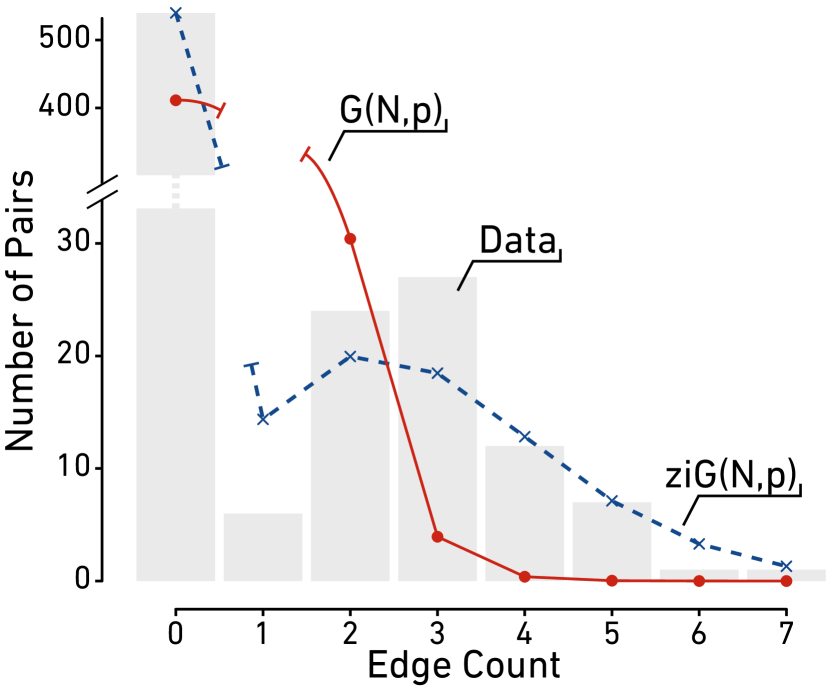
(a)

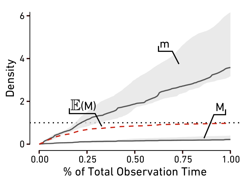
(b)

Figure 1: Empirical multi-edge networks are sparse. Traditional multi-edge models like the G(N,p) struggle to reflect real-world data characteristics. (a) edge count distribution in Zachary’s Karate Club showing bimodality. The red solid line represents the G(N,p) prediction and the blue dashed line its zero-inflated counterpart. (b) In grey, the number of multi-edges per pair $m/\binom{N}{2}$ and the fraction of connected node pairs $M/\binom{N}{2}$ over time, averaged over all Sociopatterns datasets. While $m$ rises sharply, $M$ exhibits a steadier growth, indicating that most interactions occur among existing pairs. The dashed red line denotes the expected fraction of connected pairs according to the G(N,p) model defined by the corresponding $m$ value. Note that while the model quickly predicts a fully connected network, the empirical network remains sparse.

1.1 Multi-edge network models

Multi-edge network models serve as generative stochastic frameworks that not only capture the presence of edges between nodes but also quantify the number of edges observed for each node pair. These models are crucial for understanding the complex structures and dynamics of real-world networks.

Broadly, multi-edge network models fall into three main categories: micro-canonical [32, 18], Poisson [31, 23], and Hypergeometric [6, 4]. Each category offers a different level of constraint and flexibility, catering to various types of network data.

Micro-canonical models are the most constrained, defining an ensemble of networks that share specific fixed attributes, such as degree sequences or intra-block edge counts, and assigning equal probability to each network within the ensemble. In contrast, Poisson and Hypergeometric models operate within more flexible sample spaces, preserving these attributes only in expectation. The critical difference between Poisson and Hypergeometric models lies in their independence assumptions: the former treat node pairs as independent, whereas the latter do not [4]. This distinction is crucial, as it influences the applicability and performance of the models on different types of network data.

In this article, we focus on Poisson network models. The independence assumption in Poisson models simplifies the introduction of zero-inflation, which is our primary aim.

Poisson multi-edge network models rely on Poisson count processes to describe phenomena such as edge formation and node interactions. This is the case for classic extensions of the $G(N,p)$ model to multi-edge networks [15, 20], the Chung-Lu configuration model [8, 31], the classical stochastic block model and the degree-corrected stochastic block model [23], and even count-ERGM models [24].

In a Poisson count process, the probability of observing $n$ events in a fixed time interval is governed by a Poisson distribution with parameter $\lambda$:

$$\Pr(X=n)=\frac{\lambda^{n}}{n!}e^{-\lambda}\,.$$ (1)

This Poisson model assumes that the distribution of the random variable $X$ will be centred around its mean $\lambda$, with a low probability of zero occurrences, especially as $\lambda$ increases.

Poisson network models are defined as $n^{2}$ independent Poisson count processes, one for every (directed) pair of nodes in the network:

$$\Pr(\mathcal{G})=\prod_{ij}\Pr(A_{ij})=\prod_{ij}\frac{\lambda_{ij}^{A_{ij}}}{A_{ij}!}\exp(-\lambda_{ij}),$$ (2)

where $A_{ij}$ denotes the edge count between $i$ and $j$ and $\lambda_{ij}$ are parameters that can be functions of node attributes, edge attributes, or block memberships, among others. Appropriately specifying these parameters is key for capturing the heterogeneous nature of interactions within the network.

Several well-known network models are special cases of this general Poisson framework. For example, the $G(N,p)$ model for multi-edge networks corresponds to a Poisson network model where $\lambda_{ij}=p$ for all $i,j$. The Stochastic Block Model is a generalisation that introduces $B$ different $\lambda_{b}$ parameters, one for each block in the network [23]. The Chung-Lu Configuration Model, foundational to many concepts in network science like modularity [30] and degree-correction [23], also fits within this framework, featuring node-dependent parameters $\lambda_{ij}=\theta_{i}\theta_{j}$ [8, 31]. Further, the Degree-Corrected Stochastic Block Model combines aspects of both the Chung-Lu and Stochastic Block Models, with $\lambda_{ij}=\theta_{i}\theta_{j}\lambda_{b}$ [23].

1.2 Modelling zero-inflation

While Poisson network models are standard tools in multiple disciplines [23, 24, 31], they struggle to accurately represent sparse multi-edge networks [26, 7, 13, 28, 14, 29]. The expected number of connected pairs $M$ according to a Poisson network model is given by:

$$\mathbb{E}[M]=\sum_{ij}\left(1-\exp\left(-\lambda_{ij}\right)\right).$$ (3)

However, $\sum_{ij}\lambda_{ij}$ gives the expected number of multi-edges $m$ in the network. Consequently, $\mathbb{E}[M]$ saturates exponentially with $\mathbb{E}[m]$ to a fully-connected network. Hence, with a larger observed $m$, the model tends to yield fully-connected networks.

Figure 1(b) compares the sparsity of empirical multi-edge networks with the predictions of Poisson network models. We use interaction networks from the Sociopatterns repository as an example [27] , where different datasets record contacts between individuals over short time frames. With increasing observation time and data collection, the number of multi-edges $m$ grows rapidly. Yet, the growth of the number of connected node pairs $M$ is considerably slower. This suggests that individuals predominantly interact within their existing social circles, limiting the number of new interactions over short periods. The dashed line in the plot shows the predicted number of connected pairs according to Eq. 3. As discussed above, with an increasing number of multi-edges $m$, the number of connected pairs quickly saturates to a fully connected network, deviating from the empirical data.

The observed count distribution, instead, shows a strong bimodality, characterised by peaks at zero and around some $\hat{\lambda}$ value. Even the well-known example of Zachary’s Karate Club network exhibits this bimodal distribution, as illustrated in Fig. 1(a). Zachary’s Karate Club represents the social interactions within a karate club. When examining the distribution of interactions in this network, we observe a significant number of disconnected node pairs, even when considering the existence of smaller groups, exemplifying the zero-inflation phenomenon.

Zero-inflated models [26] have been developed to mitigate this issue. These models are a mixture of a binary process for generating zeros and a Poisson count process for generating the counts. The probability mass function is given by:

$$\Pr(X=n)=(1-q)\delta_{0}(n)+q\frac{\lambda^{n}}{n!}e^{-\lambda}\,.$$ (4)

Here, $q\in[0,1]$ is the mixture weight, and $\delta_{0}(n)$ is the Kronecker delta function, which is 1 when $n=0$ and 0 otherwise. The term $(1-q)$ accounts for the excess zeros that are not explained by the Poisson process, providing a more accurate model for data like the one in Fig. 1(a).

In addition to zero-inflated models, hurdle models provide another approach to address count data with excess zeroes [17]. While zero-inflated models combine a binary process for zero counts with a Poisson process for positive counts, hurdle models treat zeros and positive counts as outcomes of two distinct processes. Specifically, a hurdle model first uses a binary process to determine whether an interaction occurs (i.e., whether the count is zero or positive), and then applies a truncated Poisson process for positive counts. This separation ensures that zeros are generated differently than positive counts, which can offer advantages in terms of model identifiability and interpretability [29]. However, this assumption implies that sparsity is only generated by the hurdle process, and not by low interaction rates. Such a strict assumption may not always hold true, especially in cases where modelling the interplay between low interaction rates and zero-inflation is critical [17].

In this article, we choose to focus only on zero-inflation as a way to model sparsity in complex networks. In the following section, we detail how zero-inflation is incorporated in Poisson network models and how to perform the inference of the parameters from data. Nevertheless, most of the results shown apply in a similar way to hurdle models [17].

Parameter Estimation

Throughout this article, we consistently employ a variation on the method of moments for parameter inference. This approach involves setting the first moments of the respective models to observed quantities—such as the number of edges, number of links, and degree sequences—from a given network. This consistency in methodology facilitates a coherent comparison across different models and allows for a clear understanding of their individual and comparative characteristics.

Often, though, we would like to obtain the maximum likelihood estimate (MLE) of the model parameters. Unfortunately, MLE presents significant challenges for zero-inflated models, a complexity underscored by the existing literature [34, 2, 9]. The inherent difficulty arises particularly in the context of network models, given the increased dimensionality. The primary reason for this complexity is that a maximum likelihood estimate of the mixture probability in Eq. 4 involves a logarithm of sums, a form that does not lend itself to simplification or easy manipulation with standard tools. Consequently, optimising the log-likelihood function usually requires a numerical approach. In these cases, the estimates obtained by the methods-of-moments serve as initial values for the numerical MLE optimisation.

2 Zero-Inflating Poisson Network Models

2.1 Zero-Inflated $G(N,p)$ Model (zi-$G(N,p)$)

The $G(N,p)$ model is one of the foundational generative models for networks and among the simplest. It is characterised solely by a parameter $p$, which determines the expected number of edges in a network realisation [20]. In this model, interactions between different node pairs are assumed to be independent and identically distributed.

For the multi-edge variant of the $G(N,p)$ model, we set $\lambda_{ij}=p$ in Eq. 2 for all node pairs. The expected number of connected node pairs—henceforth denoted as links—in a network realisation is then given by:

$$\mathbb{E}(M|p)=\sum_{ij}(1-e^{-p})=N^{2}-N^{2}e^{-p}\,,$$ (5)

where $N$ represents the number of nodes, considering a loopy directed network. This model reveals its limitation in representing sparse multi-edge networks, as $\mathbb{E}(M|p)$ approaches $N^{2}$ with increasing $p$.

To better model sparse networks, we integrate zero-inflation into the edge probabilities using Eq. 4. The zero-inflated $G(N,p)$ model is defined by:

$$\Pr(\mathcal{G}|p,q)=\prod_{ij}\left((1-q)\delta_{0}(A_{ij})+q\frac{p^{A_{ij}}}{A_{ij}!}e^{-p}\right).$$ (6)

Incorporating zero-inflation, we calculate the expected number of interactions (edges) $\mathbb{E}(m|p,q)$ and the expected number of links $\mathbb{E}(M|p,q)$ as follows:

$$\mathbb{E}(m|p,q) =qpN^{2}\,,$$ (7)

$$\mathbb{E}(M|p,q) =qN^{2}-N^{2}qe^{-p}\,.$$ (8)

To estimate the parameters $p$ and $q$ from observed data, we use the method of moments, matching these expected values to the observed counts of interactions and links, $\widehat{m}$ and $\widehat{M}$, respectively:

$$\mathbb{E}(m|p,q):=\widehat{m}\,,\qquad\mathbb{E}(M|p,q):=\widehat{M}\,.$$ (9)

Solving for $p$ and $q$, we derive:

$$\widehat{p}=\frac{\widehat{m}}{N^{2}q}\,,\qquad\widehat{q}=\frac{\widehat{m}\widehat{M}}{N^{2}(\widehat{m}+\widehat{M}\mathcal{W}\left[-\frac{\widehat{m}e^{-\frac{\widehat{m}}{\widehat{M}}}}{\widehat{M}}\right])}\,,$$ (10)

where $\mathcal{W}[z]$ represents Lambert’s W function, solving $we^{w}=z$ [26].

2.2 Zero-Inflated Stochastic Block Model (zi-SBM)

Building on the $G(N,p)$ model, the Stochastic Block Model (SBM) introduces a richer representation of network structures by distinguishing distinct blocks in the network, each characterised by a unique edge probability [22, 1]. This model captures community structures within networks. Nodes are assigned to one of $B$ different groups, and the probability of interactions between nodes $i$ and $j$ in groups $b_{i}$ and $b_{j}$, respectively, is determined by a block-specific parameter $\lambda_{b_{i}b_{j}}$.

To accommodate potential sparsity of interactions within different blocks, we detail the zero-inflated version of the SBM, denoted as zi-SBM. The model is defined by the following probability distribution:

$$\Pr(\mathcal{G}|\boldsymbol{\lambda},\boldsymbol{q})=\prod_{ij}\left((1-q_{b_{i}b_{j}})\delta_{0}(A_{ij})+q_{b_{i}b_{j}}\frac{\lambda_{b_{i}b_{j}}^{A_{ij}}}{A_{ij}!}\exp(-\lambda_{b_{i}b_{j}})\right),$$ (11)

where each block $(b,d)$ is associated with a unique mixture parameter $q_{bd}$, allowing for block-specific zero-inflation.

The expected number of interactions $m_{bd}$ and links $M_{bd}$ in the zi-SBM are given by:

$$\mathbb{E}(m_{bd}|\boldsymbol{\lambda},\boldsymbol{q}) =q_{bd}\lambda_{bd}N_{b}N_{d},$$ (12)

$$\mathbb{E}(M|\boldsymbol{\lambda},\boldsymbol{q}) =\sum_{bd}N_{b}N_{d}q_{bd}(1-e^{-\lambda_{bd}}),$$ (13)

where $N_{b}$ denotes the number of nodes in group $b$.

For parameter inference, we equate the first moments of the distribution to the observed values $\widehat{m}_{bd}$ and $\widehat{M}_{bd}$:

$$\mathbb{E}(m_{bd}|\lambda_{bd},q_{bd}):=\widehat{m}_{bd},\qquad\mathbb{E}(M_{bd}|\lambda_{bd},q_{bd}):=\widehat{M}_{bd}.$$ (14)

Solving Eq. 14, we find:

$$\widehat{\lambda}_{bd}=\frac{\widehat{m}_{bd}}{q_{bd}N_{b}N_{d}}.$$ (15)

A closed-form solution for $\widehat{q}_{bd}$ is not readily available. Nonetheless, the values of $\widehat{q}_{bd}$ can be determined by numerically solving the set of $B^{2}$ independent equations given in Eq. 14.

Dong et al. [13] proposed a variational-EM algorithm for parameter estimation in the special case of a multilayer zero-inflated stochastic block model. This algorithm efficiently estimates the community labels and model parameters, handling the sparsity and correlations in multilayer networks. The method proposed demonstrates effectiveness in capturing complex interaction patterns through extensive simulations and real-world case studies.

2.3 Zero-Inflated Configuration Model (zi-CLCM)

While both the $G(N,p)$ and SBM models offer valuable insights, they fall short in encoding node heterogeneities. Configuration models fill this gap by introducing a parameterisation that accounts for degree heterogeneities [18]. In the framework of Poisson models, the Chung-Lu configuration model (CLCM) achieves this by expressing the general parameters $\lambda_{ij}$ as $\theta^{\text{out}}_{i}\theta^{\text{in}}_{j}$, a product node-parameters [8, 31]. For undirected networks, we have $\boldsymbol{\theta^{\text{out}}}=\boldsymbol{\theta^{\text{in}}}=\boldsymbol{\theta}$.

Incorporating zero-inflation into the CLCM results in the Zero-Inflated Chung-Lu Configuration Model (zi-CLCM). The model is described by the probability distribution:

$$\Pr(\mathcal{G}|\boldsymbol{\theta},q)=\prod_{ij}\left((1-q)\,\delta_{0}(A_{ij})+q\,\frac{(\theta^{\text{out}}_{i}\theta^{\text{in}}_{j})^{A_{ij}}}{A_{ij}!}\exp(-\theta^{\text{out}}_{i}\theta^{\text{in}}_{j})\right).$$ (16)

It is important to note that the model parameters appear always in pairs. This means that they are defined modulo constants. This characteristic requires fixing a constraint that ensures a unique solution to the inference problem. A common approach is to fix the expected number of interactions in the network:

$$\mathbb{E}(m|\boldsymbol{\theta},q)=q\,\sum_{ij}\theta^{\text{out}}_{i}\theta^{\text{in}}_{j}\,.$$ (17)

To infer the parameters of the network model $q$, $\boldsymbol{\theta^{\text{out}}}$, and $\boldsymbol{\theta^{\text{in}}}$, we set four different moments to observed values:

$$\mathbb{E}(m|\boldsymbol{\theta},q):=\widehat{m},\quad\mathbb{E}(M|\boldsymbol{\theta},q):=\widehat{M},\quad\forall i:\;\mathbb{E}(k^{\text{out}}_{i}|\boldsymbol{\theta},q):=\widehat{k^{\text{out}}_{i}},\quad\forall i:\;\mathbb{E}(k^{\text{in}}_{i}|\boldsymbol{\theta},q):=\widehat{k^{\text{in}}_{i}},$$ (18)

where $\widehat{m}$ denotes the number of interactions in an observed network, $\widehat{M}$ represents its number of links, and $\widehat{k^{\text{out}}_{i}}$ and $\widehat{k^{\text{in}}_{i}}$ the observed out- and in-degrees of $i$.

The expected degree sequences and the number of links from the model are given by:

$$\mathbb{E}(k^{\text{out}}_{i}|\boldsymbol{\theta},q)=q\,\theta^{\text{out}}_{i}\sum_{j}\theta^{\text{in}}_{j},\qquad\mathbb{E}(k^{\text{in}}_{i}|\boldsymbol{\theta},q)=q\,\theta^{\text{in}}_{i}\sum_{j}\theta^{\text{out}}_{j},$$ (19)

$$\mathbb{E}(M|\boldsymbol{\theta},q)=q\,N^{2}-q\,\sum_{ij}e^{-\theta^{\text{out}}_{i}\theta^{\text{in}}_{j}}\,.$$ (20)

Fixing the expected number of interactions to $\widehat{m}$, we obtain a constraint for the L1-norm of the parameter vectors $\boldsymbol{\theta^{\text{out}}}$ and $\boldsymbol{\theta^{\text{in}}}$:

$$\sum_{i}\theta^{\star}_{i}=\sqrt{\frac{\widehat{m}}{q}}.$$ (21)

This constraint ties the expected number of interactions in the network to the node-specific parameters, allowing their inference.

From Eq. 21 and Eq. 19, we derive expressions for $\widehat{\theta^{\star}_{i}}$ as functions of $q$ and the observed degrees $\widehat{k^{\text{out}}_{i}}$ and $\widehat{k^{\text{in}}_{i}}$:

$$\widehat{\theta^{\star}_{i}}=\frac{\widehat{k^{\star}_{i}}}{\sqrt{\widehat{m}q}}\,.$$ (22)

Lastly, substituting Eq. 22 into Eq. 20 leads to an explicit equation for $\widehat{q}$:

$$\widehat{q}\,\left(N^{2}-\sum_{ij}e^{-\frac{\widehat{k^{\text{out}}_{i}}\widehat{k^{\text{in}}_{j}}}{\widehat{m}\widehat{q}}}\right)=\widehat{M}.$$ (23)

Solving numerically for $\widehat{q}$ allows the estimation of all model parameters.

2.4 Zero-Inflated Degree-Corrected Stochastic Block Model (zi-DCSBM)

We finally discuss the Zero-Inflated Degree Corrected Stochastic Block Model (zi-DCSBM). As for the standard degree-corrected stochastic block model [23], it incorporates both node heterogeneity and block structure into a single comprehensive model, combining the features of the zi-CLCM and the zi-SBM. The introduction of block-specific zero-inflation parameters $q_{bd}$, constituting the vector $\boldsymbol{q}$, allows the model to account for varying levels of zero-inflation across different blocks. By parametrising Eq. 2 with $\lambda_{ij}=\theta^{\text{out}}_{i}\theta^{\text{in}}_{j}\lambda_{b_{i}b_{j}}$, we derive the following probability distribution:

$$\Pr(\mathcal{G}|\boldsymbol{\theta},\boldsymbol{\lambda},\boldsymbol{q})=\prod_{ij}\left((1-q_{b_{i}b_{j}})\,\delta_{0}(A_{ij})+q_{b_{i}b_{j}}\,\frac{(\theta^{\text{out}}_{i}\theta^{\text{in}}_{j}\lambda_{b_{i}b_{j}})^{A_{ij}}}{A_{ij}!}\exp(-\theta^{\text{out}}_{i}\theta^{\text{in}}_{j}\lambda_{b_{i}b_{j}})\right).$$ (24)

In order to infer the model parameters, we employ the method of moments, setting the first moments of the model to their observed counterparts in a given network. The expected values of the number of interactions, node degrees, and links for each block are defined as follows:

$$\mathbb{E}(m_{bd}|\boldsymbol{\theta},\boldsymbol{\lambda},\boldsymbol{q})=q_{bd}\lambda_{bd}\sum_{i\in b}\theta^{\text{out}}_{i}\sum_{j\in d}\theta^{\text{in}}_{j},$$ (25)

$$\mathbb{E}(k^{\text{out}}_{i}|\boldsymbol{\theta},\boldsymbol{q})=\theta^{\text{out}}_{i}\sum_{d}q_{b_{i}d}\lambda_{b_{i}d}\sum_{j\in d}\theta^{\text{in}}_{j},\qquad\mathbb{E}(k^{\text{in}}_{i}|\boldsymbol{\theta},\boldsymbol{q})=\theta^{\text{in}}_{i}\sum_{d}q_{b_{i}d}\lambda_{b_{i}d}\sum_{j\in d}\theta^{\text{out}}_{j},$$ (26)

$$\mathbb{E}(M_{bd}|\boldsymbol{\theta},\boldsymbol{\lambda},\boldsymbol{q})=q_{bd}\left(N_{b}N_{d}-\sum_{i\in b,j\in d}e^{-\lambda_{bd}\theta^{\text{out}}_{i}\theta^{\text{in}}_{j}}\right),$$ (27)

where $N_{b}$ denotes the number of nodes in group $b$.

Just like in the CLCM and zi-CLCM, the parameters $\boldsymbol{\theta^{\text{out}}}$ and $\boldsymbol{\theta^{\text{in}}}$ in the DCSBM and zi-DCSBM are defined modulo constants, necessitating the establishment of a constraint to ensure a unique solution to the inference problem. A common approach is to constrain the L1-norm of the node-specific parameters, i.e., $\sum_{i}\theta^{\star}_{i}\delta_{b}(b_{i})=1$. By incorporating this constraint into Eqs. 25 and 26, we obtain:

$$\mathbb{E}(m_{bd}|\boldsymbol{\theta},\boldsymbol{\lambda},\boldsymbol{q})=q_{bd}\lambda_{bd},\quad\mathbb{E}(k^{\star}_{i}|\boldsymbol{\theta},\boldsymbol{q})=\theta^{\star}_{i}\sum_{d}q_{b_{i}d}\lambda_{b_{i}d}.$$ (28)

Solving the set of equations defined by Eqs. 25 and 26 for $\boldsymbol{\lambda}$, $\boldsymbol{\theta^{\text{out}}}$, and $\boldsymbol{\theta^{\text{in}}}$ yields expressions for their estimators that depend on the mixture parameters $\boldsymbol{q}$ and observed quantities:

$$\widehat{\lambda}_{bd}=\frac{\widehat{m}_{bd}}{q_{bd}},\quad\theta^{\star}_{i}=\frac{\widehat{k^{\star}_{i}}}{\widehat{\kappa}^{\star}_{b_{i}}},$$ (29)

where $\kappa^{\text{out}}_{b_{i}}=\sum_{d}m_{b_{i}d}$ and $\kappa^{\text{in}}_{b_{i}}=\sum_{d}m_{db_{i}}$ denote the out- and in-degree of block $b_{i}$, respectively.

Finally, substituting these expressions into Eq. 27 provides a set of equations for each $q_{bd}$ and the number of links in each block $\widehat{M}_{bd}$:

$$q_{bd}\,\left(N_{b}N_{d}-\sum_{i\in b,j\in d}e^{-\frac{\widehat{k^{\text{out}}_{i}}\widehat{k^{\text{in}}_{j}}}{\widehat{\kappa}^{\text{out}}_{b_{i}}\widehat{\kappa}^{\text{in}}_{b_{j}}}\frac{\widehat{m}_{b_{i}b_{j}}}{q_{bd}}}\right)=\widehat{M}_{bd}.$$ (30)

Numerically solving this set of $B^{2}$ independent equations yields estimates for all model parameters.

Motalebi et al. [29] discussed the zi-DCSBM in comparison with a hurdle version of the DCSBM. The probability distribution of the hurdle-DCSBM can be written as

$$\Pr(\mathcal{G}|\boldsymbol{\theta},\boldsymbol{\lambda},\boldsymbol{q})=\prod_{ij}\begin{cases}(1-q_{b_{i}b_{j}})\quad\text{if }A_{ij}=0\,,\\ q_{b_{i}b_{j}}\,\frac{(\theta^{\text{out}}_{i}\theta^{\text{in}}_{j}\lambda_{b_{i}b_{j}})^{A_{ij}}\exp(-\theta^{\text{out}}_{i}\theta^{\text{in}}_{j}\lambda_{b_{i}b_{j}})}{A_{ij}!\left(1-\exp(-\theta^{\text{out}}_{i}\theta^{\text{in}}_{j}\lambda_{b_{i}b_{j}})\right)}\quad\text{if }A_{ij}>0\,,\end{cases}$$ (31)

where the role of the model parameters is the same as in the case of the zi-DCSBM. The primary difference between these two models lies in their approach to handling sparsity: zero-inflation accounts for excess zeros by introducing a separate zero-generating process, while hurdle models treat zeros and positive counts as generated by two distinct processes. Hurdle models offer advantages in terms of identifiability because they eliminate the ambiguity between zero counts and low interaction rates. However, this means that sparsity, or disconnected pairs, is solely due to the hurdle process and not from inherently low interaction rates, which may limit their appropriateness for many applications [17].

Considerations about community detection

So far, we have presupposed that the partitioning of nodes into distinct groups is given. Nevertheless, community detection can be performed using the zero-inflated model, thereby assigning labels endogenously to the nodes based on interaction and link data. Community detection methodologies can be broadly categorised into two types: those based on quality functions [30] and those rooted in Maximum Likelihood Estimation (MLE) principles [33].

The former can be seamlessly integrated with zero-inflated models. This integration necessitates the definition of a suitable partition quality function, which can then be optimised using the parameter estimation defined herein. A classical example of this approach is modularity optimisation [30], where the partition quality function $Q$ is given by the equation:

$$Q=\frac{1}{m}\sum_{ij}\left[A_{ij}-\frac{k^{\text{out}}_{i}k^{\text{in}}_{j}}{m}\right]\delta(c_{i},c_{j}),$$ (32)

where $A_{ij}$ represents the adjacency matrix, $k_{i}$ and $k_{j}$ are the degrees of nodes $i$ and $j$, $m$ is the total number of edges, $c_{i}$ and $c_{j}$ are the communities of nodes $i$ and $j$, and $\delta$ is the Kronecker delta function. In this scenario, one would replace the expectation term $\frac{k^{\text{out}}_{i}k^{\text{in}}_{j}}{m}$ within the modularity function originating from the Chung-Lu model with that from the zi-CLCM. However, a close inspection reveals that the expected number of edges between a pair remains consistent across both models, as $q_{b_{i}b_{j}}\theta^{\text{out}}_{i}\theta^{\text{in}}_{j}\lambda_{b_{i}b_{j}}=q_{b_{i}b_{j}}\frac{k^{\text{out}}_{i}k^{\text{in}}_{j}}{mq_{b_{i}b_{j}}}=\frac{k^{\text{out}}_{i}k^{\text{in}}_{j}}{m_{b_{i}b_{j}}}$. Consequently, community detection through modularity optimisation in zero-inflated models yields analogous results to scenarios where zero-inflation is not considered.

The latter category of community detection instead, exemplified by methods utilising information theory to assess community quality, requires the computation of the MLE of the model and potentially the integration of the likelihood function to eliminate continuous parameters like $\theta^{\star}$ and $q$ (see e.g., [33]). Unfortunately, performing these integrals analytically is not possible, because of the structure of the mixture probability. A numerical solution may exist, but the development of such methods and the assessment of their divergence from the standard non-zero-inflated DCSBM fall outside the scope of this article and warrant dedicated exploration in future research.

3 Performance of Zero-Inflated Multi-Edge Models

Table 1: Summary of Datasets. $N$ is the number of nodes, $M$ is the number of unique links (i.e., connected pairs), $m$ is the number of multi-edges, $d$ is the density (fraction of connected pairs), $\rho$ is the multi-edge density (average number of multi-edges per pair of nodes). Note how all datasets except for BB are very sparse (i.e., $d\ll 1$) despite the large $\rho$.

Dataset	Type	$N$	$M$	$m$	$d$	$\rho$	kurtosis
HS13	High-school Contacts	327	5818	188508	0.11	3.54	1244.05
SFHH	Conference Interactions	403	9565	70261	0.12	0.87	4109.62
HS12	High-school Contacts	180	2220	45047	0.14	2.80	712.33
WP	Workplace Contacts	92	755	9827	0.18	2.35	880.08
WP15	Workplace Contacts	217	4274	78249	0.18	3.34	695.74
HS11	High-school Contacts	126	1709	28561	0.22	3.63	725.30
Thiers11	High-school Contacts	126	1709	28561	0.22	3.63	725.30
LyonSchool	Primary School Contacts	242	8317	125773	0.29	4.31	237.41
HT09	Conference Interactions	113	2196	20818	0.35	3.29	1771.89
HO	Hospital Contacts	75	1139	32424	0.41	11.68	152
KH	Household Contacts	47	504	32643	0.47	30.20	38.38
BB	Animal Interactions	13	78	63095	1.00	808.91	10.62

The aim of this section is to investigate the limitations of Poisson multi-edge models in dealing with empirical data and to demonstrate how zero-inflation can address these issues. We benchmark our models using classical network datasets from the Sociopatterns repository [27]. These datasets, which report contacts among individuals over short time frames, typically result in sparse multi-edge networks despite a large number of recorded interactions.

The datasets encompass various social interaction scenarios, including interactions among high-school students, conference attendees, and hospital staff. Each dataset varies in terms of the number of nodes ($N$), unique links ($M$), total multi-edges ($m$), density ($d$), and multi-edge density ($\rho$). Nevertheless, most datasets exhibit low link density, i.e., $d=M/\binom{N}{2}\ll 1$, and large multi-edge density $\rho=m/\binom{N}{2}$. This indicates a sparse network structure despite the large number of recorded interactions. Such characteristics make these datasets a prominent example where classical multi-edge models are sub-optimal. As shown in Fig. 1(b), naively modelling these datasets would quickly yield fully connected network realisations, in stark contrast with the sparse structure exhibited by the empirical data.

Interestingly, sparsity is often observed together with a “heavy-taillness” of the edge count distribution [37]. The empirical distribution of edge counts displays a considerable number of outliers, i.e., unexpectedly large edge counts. We quantify this by computing the excess kurtosis of the edge count distribution.

Excess kurtosis denotes the tails’ heaviness relative to a normal distribution. Values close to 0 indicate a distribution with similar tail behaviour to the normal distribution. Positive values signify heavier tails, indicating more extreme outliers, while negative values suggest lighter tails. In other words, large positive excess kurtosis values imply a higher probability of extreme events or outliers compared to a normal distribution. The sample excess kurtosis and other basic statistics of the empirical data analysed are reported in Table 1.

3.1 DCSBM versus zi-DCSBM

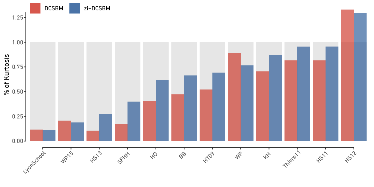
Figure 2: Percentage of sample excess kurtosis of the edge count distribution captured by DCSBM (red) and zi-DCSBM (blue) for all the Sociopatterns datasets. The expected kurtosis of each model has been computed from 100 000 realisations. Generally, zero-inflated model variants shift part of the weight of the edge count distribution to the tail, increasing the kurtosis and more closely following the empirical data.

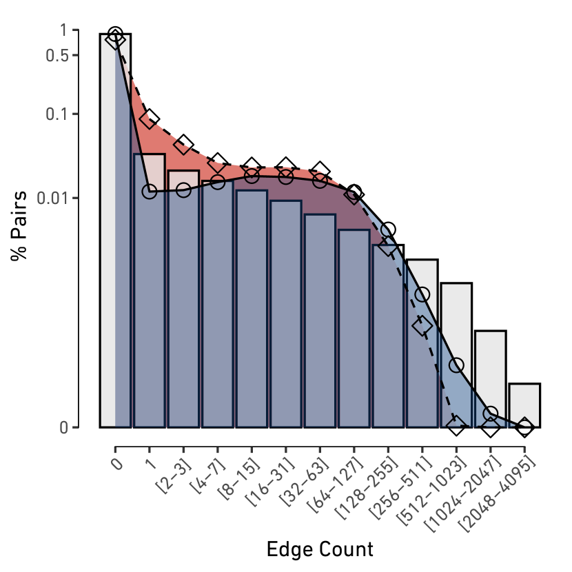
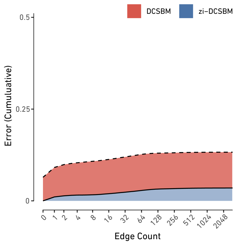
(a) Sociopatterns HS13 Dataset

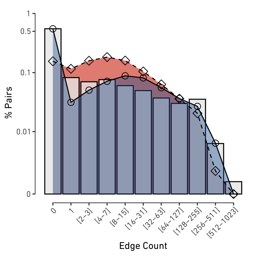
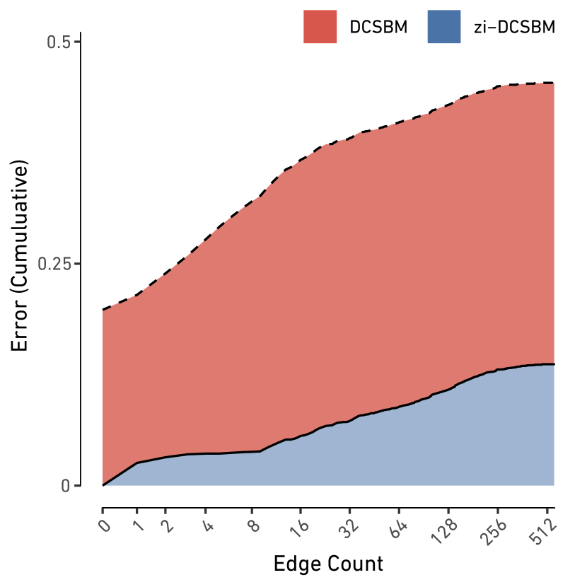
(b) Sociopatterns KH dataset

Figure 3: (top) edge count distributions for two exemplary Sociopatterns datasets (HS13 and KH). The grey bar plot shows the empirical edge count distribution. The height of a bar denotes the fraction of pairs in the network connected by a given range of multi-edges. In red, the expected edge count distribution according to a DCSBM whose blocks have been obtained by modularity maximisation. In blue, the expected edge count distribution according to its zero-inflated variant, fitted using the same blocks. (bottom) Cumulative error for the two models. In HS13, most of the difference between the two models can be attributed to the left side of the edge count distribution and pairs with low edge counts. In KH, not only is the DCSBM unable to capture the network sparsity, but it also fails to capture the heavy-tailed nature of the edge count distribution. The zi-DCSBM provides a better fit in both cases.

Among the models considered in this study, degree-corrected stochastic block models (DCSBM) are the most general due to their capability to accommodate both group-level and node-level heterogeneity. Consequently, our comparison focuses on the zero-inflated and classical variants of DCSBM. To maintain simplicity, we opt to infer the blocks in the models utilising the Leiden modularity maximisation algorithm [36]. Modularity, as previously mentioned, relies on the expected edge count derived from an underlying null-model, typically a configuration model. Given that classical and zero-inflated model pairs share the same expectation, modularity assumes an identical form for both. Hence, we can utilise identical blocks for both models. While maximum likelihood optimisation offers the potential for superior models overall, the blocks identified for classical and zero-inflated models are not necessarily the same. For the purpose of comparing how DCSBM and zi-DCSBM contend with sparse multi-edge networks, employing the same blocks allows us to better understand the differences between the two models. Therefore, we proceed with modularity-inferred blocks.

Excess Kurtosis

In Fig. 2, we plot the percentage of sample excess kurtosis in the edge count distribution captured by the DCSBM (red) and zi-DCSBM (blue). The plot primarily serves as a means to compare the excess kurtosis between the two models. Generally, zero-inflated model variants allow for a shift in part of the weight of the edge count distribution from the centre towards the tail, thereby (i) increasing the kurtosis and (ii) more closely following the empirical data. In the plot, we can see that zero-inflated models mostly yield higher kurtosis where the empirical data has particularly high sample kurtosis. This indicates the presence of more extreme edge counts compared to the standard model variants, better reproducing the empirical data.

Sparsity

When sparsity mainly arises between groups, block models—even without zero-inflation—may appear sufficient to capture sparsity. However, they are nevertheless outperformed by their zero-inflated variants. An illustrative example is provided by the HS13 dataset in Fig. 3(a). Where the number of multi-edges is large, DCSBM tends to produce numerous connected pairs with low edge counts. This contrasts with the empirical data, where fewer pairs tend to be connected but with larger edge counts.

In Fig. 3(a) (top), the empirical distribution of edge counts is depicted as a bar plot alongside the expected edge count distribution of DCSBM (shown in red). It is notable that the bulk of the weight in the distribution of DCSBM is concentrated at small positive counts, thus significantly underrepresenting large counts. Conversely, the zi-DCSBM, fitted with the same blocks, is capable of shifting the distribution (shown in blue in the plot) towards larger counts.

Figure 3(a) (bottom) illustrates the cumulative error over the different edge count values. It quantifies the discrepancy between the observed distribution and the expected distribution according to the models. The cumulative error represents the percentage of node pairs with a given edge count in the data compared to those expected in the model. In the case of HS13, for low counts there is a considerable difference between the DCSBM and the zi-DCSBM. This difference does not grow further for larger counts.

Additionally, we can use the chi-squared goodness-of-fit statistic to quantitatively compare the distributions. The chi-squared statistic for the DCSBM is $7199.8$, while the chi-squared statistic for the zi-DCSBM is $4125.2$. The smaller statistic for the zi-DCSBM shows that the zero-inflated model provides a considerably closer match to the empirical distribution. Nevertheless, the large value of both statistics indicates that both models deviate significantly from the empirical distribution.

In other examples, multi-edges are bundled over a small number of pairs both within and between groups. In these cases, the DCSBM performs particularly poorly, as it greatly underestimates the sparsity of the graph. An example of this is provided by the KH dataset in Fig. 3(b). Again, Fig. 3(b) (top) shows the empirical distribution of edge counts as a bar plot and the expected distribution of the DCSBM in red. Here, the DCSBM is unable to even approximate the empirical distribution. The zi-DCSBM fitted with the same blocks is instead able to better follow the empirical distribution (in blue in the plot). Such a large difference can be easily seen in Fig. 3(b) (bottom). The cumulative error for the DCSBM starts higher and grows much faster than in the zi-DCSBM case.

These results can be confirmed quantitatively by computing the chi-squared goodness-of-fit statistics. In the case of the DCSBM, we get $1442.7$. The zi-DCSBM gives $175.91$, nearly an order of magnitude smaller than the non zero-inflated model. This supports the qualitative assessment obtained from Fig. 3(b). In the supplementary information A, we provide as supplementary figures the equivalents of Figs. 3(a) and 3(b) for the remaining 10 Sociopatterns datasets.

The KH dataset allows for further investigation of the role of zero-inflation on network models. On the left of Fig. 4, the empirical network is visualised as a multi-edge graph. The ‘lens’ plots in the centre of the figure show two realisations from the DCSBM (bottom) and zi-DCSBM (top). It is easy to visually glean what is quantified in Fig. 3. The DCSBM yields much denser realisations, i.e., with a higher fraction of connected pairs, compared to both its zero-inflated variant and the empirical data. The adjacency matrices on the right side of Fig. 4 further confirm this. The adjacency matrix of the DCSBM realisation is much denser than either its zero-inflated counterpart or the empirical one.

Finally, the structure of a network has a significant impact on the dynamics running on it, influencing processes such as information diffusion and opinion formation. In denser networks, diffusion processes occur more rapidly. In the supplementary information B, we show that the DCSBM greatly overestimates the diffusion speed compared to the empirical data. Conversely, its zero-inflated counterpart consistently mitigates this issue by better preserving the structure of the empirical networks.

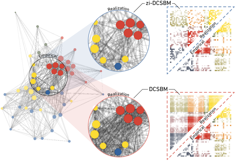
Figure 4: Comparison of the DCSBM and zi-DCSBM fits for the KH dataset. On the left side, the network is visualised as a multi-graph with parallel edges denoting multi-edges in log10 base (i.e., 1 edge represents one interaction, 2 parallel edges represent 10 interactions, and so on). Nodes are coloured according to the labels inferred by modularity maximisation. The “lens” plots show a random realisation from the DCSBM (bottom) and zi-DCSBM (top). On the right, the adjacency matrices of the random realizations are visualised against the empirical network. These plots clearly highlight how the DCSBM fails to capture the sparsity of the empirical data.

4 Discussion

Our study reveals significant limitations of classical multi-edge network models and the potential of zero-inflated models to overcome these challenges. We have shown that empirical multi-edge networks tend to be sparse despite having a large number of edges. This sparsity means that many edges are concentrated on a few node pairs, resulting in edge count distributions with heavy tails. These characteristics pose considerable difficulties for traditional multi-edge network models. They often fail to capture both the sparse nature and the high heterogeneity observed in real-world networks.

To mitigate these limitations, we show how classical multi-edge network models can be extended to incorporate zero-inflation. This involves introducing a mechanism that accounts for the excess number of zeroes (disconnected pairs) observed in empirical data. Zero-inflation not only helps in reproducing network sparsity but also improves the modelling of heavy-tailed edge count distributions. It achieves this by reducing the formation of many pairs with low edge counts in favour of a few pairs with high edge counts. This effectively shifts part of the weight of the edge count distribution towards larger counts. Failing to account for this ubiquitous property of real-world networks can lead to significant misrepresentation of network structures and dynamics.

Our results indicate that while zero-inflation significantly enhances the fit of the models to empirical data, there remain areas for improvement. In this article, we have chosen to employ modularity maximisation to infer “model-independent” node labels. This approach allowed us to evaluate the advantages of zero-inflated models compared to their classical counterparts without the confounding effects of differing block structure. However, developing block inference algorithms tailored for zero-inflated models will yield more accurate representations of network structures. This is particularly important because the blocks derived from modularity maximisation, while useful, do not always capture the full complexity of empirical networks nor can they fully exploit the advantages of zero-inflation. Moreover, zero-inflated Poisson models are limited by the restrictive nature of the Poisson distribution. In particular, Poisson models may not adequately account for over-dispersion—a common feature of count data [37]. Employing more general distributions, such as negative binomial or generalised hypergeometric distributions, can better handle over-dispersion and improve model fit [7, 13].

Our findings suggest that zero-inflated models provide a more detailed understanding of network structures, capturing both the sparsity and the extreme events reflected in the data. This aligns with the need for accurate models in various applications, such as optimising distribution systems, understanding disease spread, and analysing social behaviours. In our study, the example networks are so sparse that the necessity of zero-inflation is evident. However, in less extreme cases, determining the need for zero-inflation versus an appropriate choice of block structure becomes essential. To address this, appropriate likelihood-ratio tests and model comparison techniques have been developed for various models [7, 29, 13, 5]. These methods can help ascertain the necessity of zero-inflation by comparing the fit and performance of different models on the same dataset.

Our work bridges a critical gap in network modelling by systematically introducing zero-inflation to classical multi-edge models. This offers a more accurate framework for analysing empirical networks, thus enhancing the potential for network science to contribute to a wide range of complex systems.

Aknowledgements

The authors thank Prof. Frank Schweitzer for his support and Dr. Giacomo Vaccario for useful discussions. G.A. acknowledges funding from SNF Grant n.192746.

References

- Aicher et al. [2015] Aicher, C.; Jacobs, A. Z.; Clauset, A. (2015). Learning latent block structure in weighted networks. Journal of Complex Networks 3, 221–248.
- Ali [2022] Ali, E. (2022). A simulation-based study of ZIP regression with various zero-inflated submodels. Communications in Statistics - Simulation and Computation 53, 642–657.
- Amico et al. [2024] Amico, A.; Verginer, L.; Casiraghi, G.; Vaccario, G.; Schweitzer, F. (2024). Adapting to disruptions: Managing supply chain resilience through product rerouting. Science Advances 10, eadj1194.
- Casiraghi [2019] Casiraghi, G. (2019). The block-constrained configuration model. Applied Network Science 4, 1–22.
- Casiraghi [2021] Casiraghi, G. (2021). The likelihood-ratio test for multi-edge network models. Journal of Physics: Complexity 2, 035012.
- Casiraghi and Nanumyan [2021] Casiraghi, G.; Nanumyan, V. (2021). Configuration models as an urn problem. Scientific Reports 11, 13416.
- Choi and Ni [2023] Choi, J.; Ni, Y. (2023). Model-based Causal Discovery for Zero-Inflated Count Data. Journal of Machine Learning Research 24, 1–32.
- Chung and Lu [2002] Chung, F.; Lu, L. (2002). Connected Components in Random Graphs with Given Expected Degree Sequences. Annals of Combinatorics 6, 125–145.
- Consul and Famoye [1992] Consul, P.; Famoye, F. (1992). Generalized poisson regression model. Communications in Statistics - Theory and Methods 21, 89–109.
- Danon et al. [2011] Danon, L.; Ford, A. P.; House, T.; Jewell, C. P.; Keeling, M. J.; Roberts, G. O.; Ross, J. V.; Vernon, M. C. (2011). Networks and the Epidemiology of Infectious Disease. Interdisciplinary Perspectives on Infectious Diseases 2011, 284909.
- Darling and Norris [2005] Darling, R. W. R.; Norris, J. R. (2005). Structure of large random hypergraphs. The Annals of Applied Probability 15, 125–152.
- Decelle et al. [2011] Decelle, A.; Krzakala, F.; Moore, C.; Zdeborová, L. (2011). Asymptotic analysis of the stochastic block model for modular networks and its algorithmic applications. Physical Review E 84, 066106.
- Dong et al. [2019] Dong, H.; Chen, N.; Wang, K. (2019). Modeling and Change Detection for Count-Weighted Multilayer Networks. Technometrics 62, 184–195.
- Ebrahimi et al. [2021] Ebrahimi, S.; Reisi-Gahrooei, M.; Paynabar, K.; Mankad, S. (2021). Monitoring sparse and attributed networks with online Hurdle models. IISE Transactions 54, 91–104.
- Erdős and Rényi [1959] Erdős, P.; Rényi, A. (1959). On random graphs. I. Publicationes Mathematicae Debrecen 6, 290–297.
- Faloutsos et al. [2004] Faloutsos, C.; McCurley, K. S.; Tomkins, A. (2004). Connection subgraphs in social networks. In: SIAM International Conference on Data Mining, Workshop on Link Analysis, Counterterrorism and Security. vol. 2.
- Feng [2021] Feng, C. X. (2021). A comparison of zero-inflated and hurdle models for modeling zero-inflated count data. Journal of Statistical Distributions and Applications 8, 8.
- Fosdick et al. [2018] Fosdick, B. K.; Larremore, D. B.; Nishimura, J.; Ugander, J. (2018). Configuring Random Graph Models with Fixed Degree Sequences. SIAM Review 60, 315–355.
- Freeman et al. [2004] Freeman, L.; et al. (2004). The development of social network analysis. A Study in the Sociology of Science 1, 159–167.
- Gilbert [1959] Gilbert, E. N. (1959). Random Graphs. The Annals of Mathematical Statistics 30, 1141–1144.
- Gote et al. [2023] Gote, C.; Casiraghi, G.; Schweitzer, F.; Scholtes, I. (2023). Predicting variable-length paths in networked systems using multi-order generative models. Applied Network Science 8, 68.
- Holland et al. [1983] Holland, P. W.; Laskey, K. B.; Leinhardt, S. (1983). Stochastic blockmodels: First steps. Social Networks 5, 109–137.
- Karrer and Newman [2011] Karrer, B.; Newman, M. E. J. (2011). Stochastic blockmodels and community structure in networks. Physical Review E 83, 16107.
- Krivitsky [2012] Krivitsky, P. N. (2012). Exponential-family random graph models for valued networks. Electronic Journal of Statistics 6, 1100–1128.
- Krivitsky et al. [2011] Krivitsky, P. N.; Handcock, M. S.; Morris, M. (2011). Adjusting for network size and composition effects in exponential-family random graph models. Statistical Methodology 8, 319–339.
- Lambert [1992] Lambert, D. (1992). Zero-Inflated Poisson Regression, with an Application to Defects in Manufacturing. Technometrics 34, 1–14.
- Mastrandrea et al. [2015] Mastrandrea, R.; Fournet, J.; Barrat, A. (2015). Contact Patterns in a High School: A Comparison between Data Collected Using Wearable Sensors, Contact Diaries and Friendship Surveys. PLOS ONE 10, e0136497.
- Motalebi et al. [2021a] Motalebi, N.; Owlia, M. S.; Amiri, A.; Fallahnezhad, M. S. (2021a). Monitoring social networks based on Zero-inflated Poisson regression model. Communications in Statistics - Theory and Methods 52, 2099–2115.
- Motalebi et al. [2021b] Motalebi, N.; Stevens, N. T.; Steiner, S. H. (2021b). Hurdle Blockmodels for Sparse Network Modeling. The American Statistician 75, 383–393.
- Newman and Girvan [2004] Newman, M. E. J.; Girvan, M. (2004). Finding and evaluating community structure in networks. Physical Review E 69, 026113.
- Norros and Reittu [2006] Norros, I.; Reittu, H. (2006). On a conditionally Poissonian graph process. Advances in Applied Probability 38, 59–75.
- Peixoto [2013] Peixoto, T. P. (2013). Parsimonious Module Inference in Large Networks. Physical Review Letters 110, 148701.
- Peixoto [2017] Peixoto, T. P. (2017). Nonparametric Bayesian inference of the microcanonical stochastic block model. Physical Review E 95, 012317.
- Sari et al. [2021] Sari, D. N.; Purhadi, P.; Rahayu, S. P.; Irhamah, I. (2021). Estimation and Hypothesis Testing for the Parameters of Multivariate Zero Inflated Generalized Poisson Regression Model. Symmetry 13, 1876.
- Scholtes [2017] Scholtes, I. (2017). When is a Network a Network?: Multi-Order Graphical Model Selection in Pathways and Temporal Networks. In: Proceedings of the 23rd ACM SIGKDD International Conference on Knowledge Discovery and Data Mining. KDD ’17, ACM.
- Traag et al. [2019] Traag, V. A.; Waltman, L.; van Eck, N. J. (2019). From Louvain to Leiden: guaranteeing well-connected communities. Scientific Reports 9, 5233.
- Yang et al. [2009] Yang, Z.; Hardin, J. W.; Addy, C. L. (2009). Testing overdispersion in the zero-inflated Poisson model. Journal of Statistical Planning and Inference 139, 3340–3353.