Fine-Grained Domain Generalization with Feature Structuralization

Abstract

Fine-grained domain generalization (FGDG) is a more challenging task than traditional DG tasks due to its small inter-class variations and relatively large intra-class disparities. When domain distribution changes, the vulnerability of subtle features leads to a severe deterioration in model performance. Nevertheless, humans inherently demonstrate the capacity for generalizing to out-of-distribution data, leveraging structured multi-granularity knowledge that emerges from discerning the commonality and specificity within categories. Likewise, we propose a Feature Structuralized Domain Generalization (FSDG) model, wherein features experience structuralization into common, specific, and confounding segments, harmoniously aligned with their relevant semantic concepts, to elevate performance in FGDG. Specifically, feature structuralization (FS) is accomplished through joint optimization of five constraints: a decorrelation function applied to disentangled segments, three constraints ensuring common feature consistency and specific feature distinctiveness, and a prediction calibration term. By imposing these stipulations, FSDG is prompted to disentangle and align features based on multi-granularity knowledge, facilitating robust subtle distinctions among categories. Extensive experimentation on three benchmarks consistently validates the superiority of FSDG over state-of-the-art counterparts, with an average improvement of 6.2% in FGDG performance. Beyond that, the explainability analysis on explicit concept matching intensity between the shared concepts among categories and the model channels, along with experiments on various mainstream model architectures, substantiates the validity of FS.

I Introduction

Deep Learning (DL) has achieved remarkable success in various visual tasks thanks to its powerful ability to learn and extract representations from data. However, most data-driven models, operating under the oversimplified assumption of independent and identically distributed (i.i.d.) scenarios, encounter obstacles when deployed in diverse contexts, often referred to as out-of-distribution (OOD) problems. The recognition capability of deep neural networks (DNNs), trained on a source domain (e.g., sketches), significantly deteriorates upon application to other target domains (e.g., the real world)  [1]. To address OOD problems, many generalization-related topics have been proposed, such as domain adaptation (DA) and domain generalization (DG). Among them, DG is a more credible setting since it does not incorporate test domain data into the training process [2]. Typically, identifying domain invariance to reduce the risk of overfitting is a viable direction of DG [3, 4]. It treats the invariance across given source domains as intrinsic generalizable features of objects [5].

However, this invariance performs sub-optimally in fine-grained domain generalization tasks (FGDG), especially in single-source scenarios. In fine-grained data, the distinctions among categories are relatively small compared to intra-class differences. DNNs tend to learn finer discriminative features when trained on fine-grained data, resulting in a worse entanglement among spurious features and object categories [6]. The OOD problems are exacerbated as the learned features grow increasingly vulnerable and fragile to distribution shifts [7]. Furthermore, collecting multi-source fine-grained data is more laborious than collecting multi-source coarse-grained data [8], and the reduced distributional diversity within a single-source training environment makes learning invariance more arduous [5]. All of these factors significantly increase the difficulty of FGDG, resulting in traditional DG methods exhibiting subpar generalization performance. Therefore, it is crucial to explore the fine-grained invariant representation capabilities of DNNs more thoroughly.

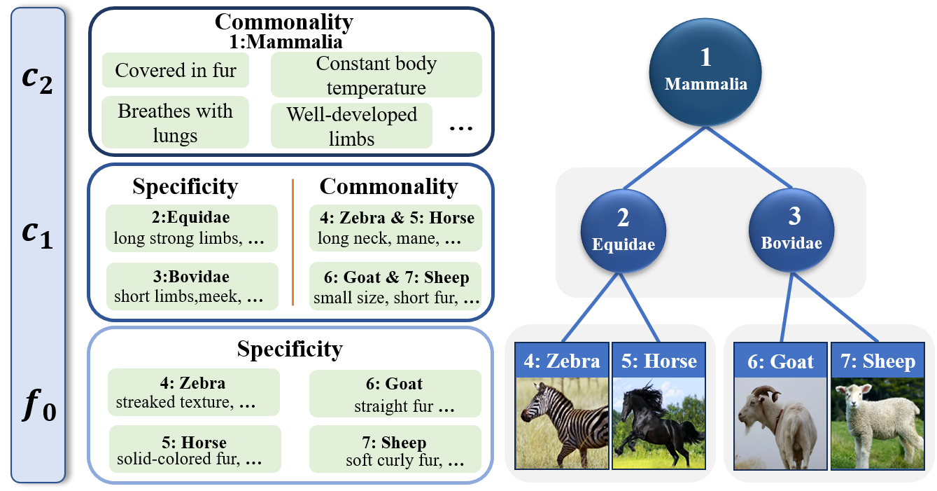
Figure 1: Instance of multi-granularity knowledge. Four animals are categorized into various classes across three granularity levels according to their commonalities and specificities.

In FGDG tasks, fine-grained categories exhibit multi-granularity structures built upon the commonalities and specificities between categories. This aspect is overlooked by previous DG methods. In contrast, humans exhibit a higher level of generalizability by leveraging these structured semantics for learning and recognizing. According to family resemblances [9], feature integration theory [10], and lexical structure [11] in cognitive psychology, when learning to recognize objects, people focus primarily on the salient targets and inductively disentangle the commonalities and specificities among them. Commonalities represent basic visual concepts, whereas specificities correspond to individual conceptual extensions. Both serve as the foundational elements for object classification and vary across distinct granularity levels [12, 13, 14]. For instance, as Fig. 1 shows, four animals can be reclassified into categories of Equidae and Bovidae based on their commonalities and specificities from a higher $c_{1}$ granularity level, respectively. At $c_{1}$ level, zebra and horse share certain characteristics, such as long necks, while manifesting specificities at fine-grained level $f_{0}$. It can be observed that the common and specific features, which constitute the intrinsic characteristics of objects, can be facilitated by incorporating multi-granularity knowledge. Understanding the commonalities and specificities between categories enhances the generalizability, as both focus more on the intrinsic features of the objects themselves.

However, a key challenge arises: how to explicitly embed these structured commonalities and specificities into DL models. In particular, it is unclear to determine what semantic basis can be used for constructing clusters of commonalities and specificities, and it is challenging to constrain them within their respective semantic clusters, as literature has discussed the unattainability of learning decoupling semantics in the absence of sufficient additional knowledge constraints [15].

To address this challenge, we propose a Feature Structuralization (FS) framework employing multi-granularity knowledge as an additional constraint for semantic disentanglement and alignment. Researches in the explainability field show that features or tokens behave as distinct semantics [16, 17, 18, 19], which implies that commonalities and specificities can be disentangled from the learned features. Acknowledging that recognition tasks predominantly seek to discern target objects in an image that encompasses target semantics and confounding, we disentangle the total semantical features learned from an image into three components, namely commonality, specificity, and confounding. Furthermore, the representations of commonalities and specificities are constrained within their respective semantic clusters with the aid of a multi-granularity knowledge structure. The collaboration between both facilitates the network in learning category invariance while preserving learning discrimination. Consequently, FS optimizes the fine-grained invariant representations as both focus more on the attributes of the objects themselves rather than on the other spurious correlations.

To formulate FS, we devise a pipeline consisting of two essential steps: disentanglement and alignment. We disentangle the three parts according to their channel indices. A decorrelation optimization function is employed to minimize the mutual information between them. Three similarity-based losses are then proposed for the alignment of common and specific parts with the aid of multi-granularity knowledge. Two of these are leveraged to pull commonalities closer across diverse granularities, while the third serves to create distance among the specific components. Furthermore, a Feature Structuralized Domain Generalization model (FSDG) is constructed by incorporating a prediction calibration method. Three model variations are expanded in conjunction with Convolutional Neural Network (CNN), Transformer, and Multi-Layer Perceptron (MLP).

In summary, the contributions of this work are as follows:

(1) We propose an FS framework to address a more difficult FGDG challenge, drawing inspiration from cognitive psychology. This novel approach integrates data and multi-granularity knowledge to structure the learned features into common, specific, and confounding parts according to their channel indices, which is in line with the analysis of explainability. FS endows the model with the ability to explicitly learn commonalities and specificities between categories.

(2) We construct a feature-structuralized model FSDG by formulating FS into a disentanglement and alignment pipeline. A disentanglement enhancement function is derived to reduce the correlation between the three segments. Three constraints are then designed to achieve semantic alignment for the common and specific components. To our knowledge, FSDG is a pioneer tailored to address FGDG issues.

(3) A CRP method is refined to substantiate the validity of FS. It statistically computes the most relevant concepts for every category, showing that FS significantly increases the explicit concept matching intensity between the shared concepts among categories and the model channels. Besides, extensive experiments on three benchmarks, along with three FSDG variants, show that FSDGs outperform their counterparts in terms of FGDG performance.

The remainder of this article is organized as follows. Section II reviews related works. Problem formulation and the proposed FS framework are presented in Section III. In Section IV, the experimental analysis of the proposed approach is presented. The explainability analysis is explored in Section V. Finally, Section VI concludes this article with a brief discussion on limitations and future work.

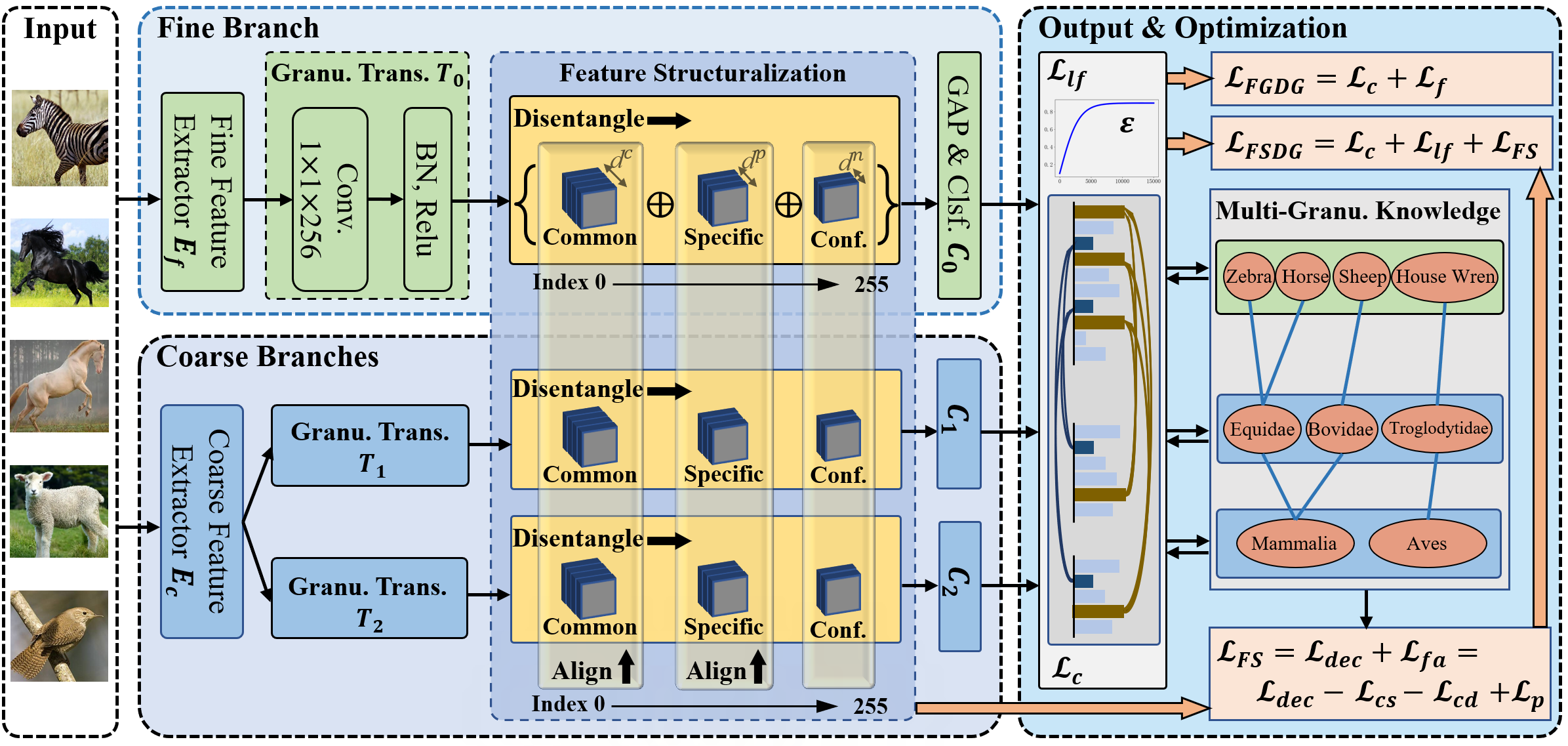
Figure 2: Illustration of the model exemplified in a three-granularity hierarchy (i.e., $G=3$). The FS module is highlighted in the middle box with solid arrows depicting the operation dimensions. $\oplus$ represents the disentanglement operator. Given five input images, FSDG outputs multi-granular results, as indicated in the right section. The box showing $\mathcal{L}_{lf}$ illustrates the alignment operation for coarse-fine predicted distributions and shows $\varepsilon$ during the training process. Conf. is an abbreviation of confounding and Granu. Trans. means the Granularity Transition Layer. The coarse branches and the FS optimization module are excluded during model inference.

II Related Work

II-A Domain Generalization

Research on alleviating OOD issues has been conducted from various perspectives [2, 20]. DA, as a straightforward solution, directly utilizes target domain data as auxiliary knowledge to train the model [7]. However, collecting or even identifying target data before deploying the model is unbearable, and when applied to a third domain, the model still encounters failures [5]. Therefore, it is more appropriate to study the DG problem without training the target domain data. In recent years, numerous DG strategies have been proposed, such as learning domain-invariant representations [21, 22], data augmentation [23, 24], optimization strategies [25, 26, 27], and disentangled representations [28].

Robust domain-invariant representations emphasize computing the consistencies across multi-source domains [5]. Rosenfeld et al. [3] acquired domain-invariant features with the help of causal analysis. Literature [29] computed a kind of rationale invariance to enhance DG performance. Data augmentation methods can be used to generate multiple domain data for single-source DG problems [30]. [31] employed adversarial training to generate images with unseen styles. Zhou et al. [23] mixed the statistics of two images in the image or feature level to generate new styles. Wang et al. [25] improved DG capability by implicitly aligning the gradient directions between the empirical risk and the perturbed loss. Zhang et al. [1] introduced a training strategy called Lookahead, which involves weight interpolation, to explore flat minima for DG issues. In [32], two separate encoders were learned in an adversarial way to capture identity and domain information, respectively. Low-rank decomposition on weight matrices is applied in [33] to identify features that are more generalizable.

However, a majority of these methods are grounded in multi-source data, without consideration of learning invariance through understanding commonalities and specificities between categories. They struggle to achieve the anticipated performance in single-source and FGDG tasks.

II-B Fine-Grained Visual Categorization

Fine-grained visual categorization (FGVC) strives to discriminate subtle distinctions between subordinate categories within the same root category [6]. It presents a formidable challenge due to the inherent dilemma of minimal inter-class variation coupled with significant intra-class variation. Researchers endeavoring to handle this problem can be classified into three main paradigms: feature enhancement-based [34], localization-based [35], and external knowledge-based methods [36]. These methods mainly focus on enhancing the fine discriminative characteristics. For example, FET-FGVC [34] proposed a feature-enhanced Transformer, cooperating with Graph Neural Networks, to improve the performance of FGVC. Zheng et al. [35] firstly localized key object parts within images and then found discriminative clues on object parts. Literature [36] incorporated object structure knowledge into the transformer to upgrade discriminative representations. As for fine-grained generalization issues, PAN [7] harnessed multi-granularity knowledge, aligning the final multi-granular predictions to improve fine-grained DA performance. WDAN [37] utilized a weighted discriminative adversarial network to release the fine-grained DA issue. However, these methods neglect feature invariance between categories, and the single-source FGDG problem has not been explored.

Compared with all aforementioned methods, FS aims to tackle the problem of single-source FGDG. Our method can be regarded as a cognition-inspired paradigm [11, 38] in which FS organizes the feature space into commonality, specificity, and confounding through multi-granularity knowledge.

III Method

In this section, we introduce our problem formulation and the details of our proposed FS framework. We illustrate how our method disentangles feature space into three parts. An aligning strategy is then adopted to achieve semantic functionalization.

III-A Problem Statement

Domain Generalization: Let $\mathcal{X}=\left\{(x)\right\}$ be the input space and $\mathcal{Y}=\left\{(y)\right\}$ the label space. In the context of DG, $\mathcal{D_{S}}=\left\{\mathcal{S}^{s}=\left\{\left(x^{s},y^{s}\right)\right\}\right\}_{s=1}^{M}$ and $\mathcal{D_{T}}=\left\{\mathcal{T}\right\}$ denote $M$ source domains and an unseen target domain, respectively. We train a model $f:\mathcal{X}\rightarrow\mathcal{Y}$ utilizing only source domain data $\mathcal{D_{S}}$. The goal of DG is to minimize the prediction error of $f$ on the unseen target domain $\mathcal{D_{T}}$. Classical DG approaches work in multi-source scenarios (i.e., $M>1$), learning invariant representations of multiple source domains. In contrast, single-source DG (i.e., $M=1$) is a more realistic problem in open environments, as it is hard to ensure that invariant features remain consistent in the target domain, especially given the limited number of available source domains for training.

Fine-Grained Domain Generalization: In the FGDG problem, a model $f$ is trained on $M$ source domains $\mathcal{D_{S}}=\left\{\mathcal{S}^{s}=\left\{\left(x^{s},y_{f}^{s},\left.y_{g}^{s}\right|_{g=1}^{G-1}\right)\right\}\right\}_{s=1}^{M}$ and tested on a target domain $\mathcal{D_{T}}=\left\{\mathcal{T}\right\}$. The label space of $\mathcal{D_{S}}$ is constructed in a multi-granular format with a total $G$-layer hierarchy (i.e., $\mathcal{Y}=\left\{(y_{f},\left.y_{g}\right|_{g=1}^{G-1})\right\}$). Traditional DG can be seen as a particular kind of FGDG whose label space has only the fine-grained labels $y_{f}$ without the coarse-grained labels $\left.y_{g}\right|_{g=1}^{G-1}$, where $g$ is a notation of granularity level and subscript $f$ represents the fine-grained content (i.e., $g=0$). The objective of FGDG is to minimize the fine-grained prediction error on the unseen target domain $\mathcal{D_{T}}$. In this paper, we enhance FGDG performance in a single-source scenario (i.e., $M=1$), taking into account a more realistic situation in which multi-source fine-grained structured data is more difficult to fabricate. Additionally, single-source FGDG can demonstrate the efficacy of our method more effectively.

Accordingly, we construct a baseline FGDG model as shown in Fig. 2. Macroscopically, feature extractors $E$ extract semantic features, followed by granularity transition layers $T$ to filter the corresponding granularity information. Finally, the Global Average Pooling (GAP) and Fully Connected (FC) classifier $C$ predict the resulting distributions. Integrating disentanglement and alignment, the FS optimization module is introduced to structuralize the features systematically.

III-B Disentanglement and Decorrelation of Three Partitions

In this paper, our objective is to enhance FGDG performance utilizing multi-granularity knowledge. In order to fully exploit this knowledge, we configure two backbones to extract coarse and fine features separately, as shown in Fig. 2. $G$ transition layers parallelly decompose the coarse and fine backbone features into features unique to each granularity, resulting in $G$ branches working in a multi-task manner. The fine branch is dedicated to identifying the fine-grained categories, while the features of coarse branches assist the fine-grained features in capturing commonalities and specificities.

Specifically, given a batch of source domain images $x\in\mathbb{R}^{B\times 3\times W\times H}$, two feature extractors $E_{c}$ and $E_{f}$ extract coarse and fine features $\mathcal{F}_{c}$ and $\mathcal{F}_{f}$, respectively. Then $\left.T_{g}\right|_{g=0}^{G-1}$ take them as input to decompose the granular features $\left.\mathcal{F}_{g}\right|_{g=0}^{G-1}$ for every granularity. For branch $g$, $\mathcal{F}_{g}$ consists of a set of features $\left\{{f}_{g}^{1},{f}_{g}^{2},\cdots,{f}_{g}^{d}\right\}$, where $d$ is the channel number of $T_{g}$. Finally, $\left.C_{g}\right|_{g=0}^{G-1}$ output the predicted logits belonging to every granularity. It is imperative to elucidate that the auxiliary coarse branches and the entire FS optimization module will be excluded during inference, signifying that the ultimate deployed model comprises exclusively the fine-grained branch. Moreover, the feasibility of training with a solitary backbone is also evident.

Features ${f}_{g}\in\mathbb{R}^{B\times 1\times w\times h}$ of CNN or tokens of Transformer represent distinctive semantics of the input images  [18, 19]. Taking CNN as an example, we obtain $d$ semantic features $\mathcal{F}_{g}$ after $T_{g}$. We disentangle them into three segments:

$$\left\{\mathcal{F}_{g}^{c},\mathcal{F}_{g}^{p},\mathcal{F}_{g}^{n}\right\}=Disentangle(\mathcal{F}_{g}),$$ (1)

where $\mathcal{F}_{g}^{c}=\left\{\left.{f}_{g}^{c,i}\right|_{i=1}^{d^{c}}\right\}$ denotes $d^{c}$ common features, $\mathcal{F}_{g}^{p}=\left\{\left.{f}_{g}^{p,i}\right|_{i=1}^{d^{p}}\right\}$ reflects the specific segment, $\mathcal{F}_{g}^{n}=\left\{\left.{f}_{g}^{n,i}\right|_{i=1}^{d^{n}}\right\}$ is the confounding part, and $d=d^{c}+d^{p}+d^{n}$, respectively.

In this paper, we disentangle features at the conceptual level according to their channel indices, as the interpretability analysis shows that channels can express various concepts [18]. This procedure is also characterized by its conciseness, practicality, and computational efficiency. It allows us to explicitly identify the index positions of the functionality of the three parts, fortifying the transparency of the model.

To enhance the degree of disentanglement from a semantic perspective, we argue that the conceptual features described in the three segments should be as independent and orthogonal as possible. We first compute the prototypes of the segments:

$$\left\{\begin{gathered}P_{g}^{c}=MEAN(F_{g}^{c},dim=1)\\ P_{g}^{p}=MEAN(F_{g}^{p},dim=1)\\ P_{g}^{n}=MEAN(F_{g}^{n},dim=1),\end{gathered}\right.$$ (2)

where $MEAN(X,dim)$ is the average operator of tensor $X$ along the $dim$ dimension, $F_{g}^{c}\in\mathbb{R}^{B\times d^{c}\times wh}$, $F_{g}^{p}$ and $F_{g}^{n}$ are slices of the stacked 3-d tensor $F_{g}\in\mathbb{R}^{B\times d\times wh}$ along the channel dimension, with extraction ratios set to $r^{c}$, $r^{p}$ and $r^{n}$. The resulted $P_{g}^{c}\in\mathbb{R}^{B\times wh}$, $P_{g}^{p}$ and $P_{g}^{n}$ are then stacked as $P_{g}^{all}\in\mathbb{R}^{B\times 3\times wh}$. The objective loss function of decorrelation among three segments is defined as

$$\mathcal{L}_{dec}=\frac{1}{B}\frac{1}{G}\sum_{b=0}^{B-1}\sum_{g=0}^{G-1}SUM({\left\langle P_{b,g}^{all},P_{b,g}^{all}\right\rangle\over\|P_{b,g}^{all}\|_{2}\|P_{b,g}^{all}\|_{2}}-\mathbf{I}),$$ (3)

where $SUM(X)$ is the summation operator among all elements of tensor $X$, and $\mathbf{I}$ is a identity matrix. Cosine similarity is utilized as the metric because it can directly quantify orthogonality. Other metrics, such as Hilbert-Schmidt independence criterion (HSIC) [39] and Euclidean distance [40], are also tested, and results are presented in Section IV.

III-C Alignment for Commonality, Specificity and Prediction

In essence, our ambition is to endow each feature with a semantic concept that can describe the common and specific parts between objects. In the real world, commonalities and specificities can be identified and utilized to distinguish different objects with the assistance of multi-granularity knowledge. In the same way, this multi-granular structure can effectively assist in identifying and aligning the learned features with those functions for DL models.

Commonality Alignment constrains the first section of features to match the common characteristics between categories. The constraint is implemented from two perspectives. Firstly, we argue that the common features within a sample should consistently manifest across diverse granularities because the intrinsic information regarding the objects remains unaffected by alterations in granularities. Secondly, we mandate the congruence of common features belonging to identical categories at the parent granularity but differing at the sub-granularity. For example, zebras and horses at the sub-granularity emerge as distinct sub-categories of the parent category Equidae while sharing certain common attributes, as shown in Fig. 1.

In particular, the output features of $\left.T_{g}\right|_{g=0}^{G-1}$ are initially stacked as a 4-d tensor $F\in\mathbb{R}^{G\times B\times d\times wh}$. All features are tokenized, resulting in $wh$ tokens in dimension $d$, which enables transformer-based variants of FS. The common slice is sequentially extracted from $F$ based on Eq. (1). The first constraint, denoted as $\mathcal{L}_{cs}$, measures how similar the common features of the same samples are across each pair of neighboring granularities. This distance is formulated as

$$S_{cs}=\frac{1}{B}\frac{1}{G-1}\sum_{b=0}^{B-1}\sum_{g=0}^{G-2}SUM({\left\langle{f}_{b,g}^{c},{f}_{b,g+1}^{c}\right\rangle\over\|{f}_{b,g}^{c}\|_{2}\|{f}_{b,g+1}^{c}\|_{2}}),$$ (4)

where ${f}_{b,g}^{c}\in\mathbb{R}^{d^{c}\times wh}$ belongs to ${g}_{th}$ granularity of ${b}_{th}$ image.

For the second constraint, we locate sub-granularity samples of every parent class, progressing from the highest parent granularity to the lowest. Given a batch of images $x$ in $\left.m_{g}\right|_{g=0}^{G-1}$ classes, the samples belonging to $q_{th}$ parent category $y_{g+1}^{q}$ are of different classes at sub-granularity $g$, denoted by $\left.x^{q,k}_{g}\right|_{k=1}^{K}$, where $k$ is the sub-category, and $K=m_{g}^{q}$ is the according number of sub-categories. For every sub-category, we compute the GAP of the obtained feature tensor $F_{B_{k,q,g}}^{c}\in\mathbb{R}^{B_{k,q,g}\times d^{c}\times wh}$ to represent the fundamental common centroid:

$$P_{k,q,g}^{c}=MEAN(GAP(F_{B_{k,q,g}}^{c}),dim=0),$$ (5)

where $B_{k,q,g}$ depicts samples that belong to $q_{th}$ category at granularity $g+1$ and $k_{th}$ sub-category at $g$. $P_{k,q,g}^{c}$ represents the centroid of the common characteristics of samples belonging to the current sub-granularity category. The second constraint, denoted as $\mathcal{L}_{cd}$, forces the sub-centroids of a given parent category to move closer. The total distance among the stacked sub-centroid tensors $P_{q,g}^{c}\in\mathbb{R}^{K\times d^{c}}$ for all parent categories and all granularities is formulated as

$$S_{cd}=\frac{1}{G-1}\frac{1}{Q_{g}}\frac{1}{K}\sum_{g=0}^{G-2}\sum_{q=0}^{Q_{g}-1}SUM({\left\langle P_{q,g}^{c},P_{q,g}^{c}\right\rangle\over\|P_{q,g}^{c}\|_{2}\|P_{q,g}^{c}\|_{2}}-\mathbf{I}),$$ (6)

where $Q_{g}$ is the number of parent categories at granularity $g$.

Specificity Alignment regulates the second group of features to match the distinctive characteristics between objects, denoted as $S_{p}$. The main idea is that the specific representations of different categories at the same granularity should be maximally distinct. We compute the specificity centroid as

$$P_{k,g}^{p}=MEAN\left(GAP\left(F_{B_{k,g}}^{p}\right),dim=0\right).$$ (7)

The total distance among the stacked centroids $P_{g}^{p}\in\mathbb{R}^{K\times d^{p}}$ for all granularities can be formulated as

$$S_{p}=\frac{1}{G-1}\frac{1}{K}\sum_{g=0}^{G-1}SUM({\left\langle P_{g}^{p},P_{g}^{p}\right\rangle\over\|P_{g}^{p}\|_{2}\|P_{g}^{p}\|_{2}}-\mathbf{I}).$$ (8)

Prediction Calibration constrains the predictions from each branch in the FSDG model to construct a granularity tree. Regarding  [7, 41], the fine-grained ground-truth labels progressively integrate with the predicted distributions at the coarse-grained branches, as shown in Fig. 2. The prediction alignment loss $\mathcal{L}_{lf}$ is designed to connect the prediction spaces of fine and coarse granularities during the training process and to optimize the fine branch. $\mathcal{L}_{lf}$ is formulated as

$$\mathcal{L}_{lf}(\left.\widehat{y}_{g}\right| {}_{g=1}^{G-1},\widehat{y}_{f},\left.y_{f}\right)$$ (9)

$$=D_{\mathrm{KL}}\left(\varepsilon y_{f}+(1-\varepsilon)\sum_{g=1}^{G-1}\frac{\widehat{y}_{g}}{G-1}\|\widehat{y}_{f}\right),$$

where $\widehat{y}_{f}={C_{f}}({T_{f}}({E_{f}}(x)))$ is the fine-grained predicted distribution, $D_{\mathrm{KL}}$ is the Kullback-Leibler divergence, $\widehat{y}_{g}={C_{g}}({T_{g}}({E_{c}}(x)))$ ($g\neq 0$), of which dimension has been extended to the same as $\widehat{y}_{f}$, is the output of coarse branches, and $\varepsilon$ controls the intensity of the coarse-grained influence on fine-grained classification. All coarse branches are trained to minimize the traditional recognition objective:

$$\mathcal{L}_{c}=\sum_{g=1}^{G-1}L_{CE}\left(\widehat{y}_{g},y_{g}\right),$$ (10)

where $L_{CE}$ represents the cross-entropy (CE) loss.

The FS is achieved by the FS objective function $\mathcal{L}_{FS}$, comprising disentanglement and alignment functions $\mathcal{L}_{dec}$ and $\mathcal{L}_{fa}$, and a prediction calibration loss $\mathcal{L}_{lf}$. $\mathcal{L}_{fa}$ maximizes the similarity of common features while minimizing the similarity of specific features. The FS objective is formulated as

$$\mathcal{L}_{FS} =\mathcal{L}_{dec}+\mathcal{L}_{fa}$$ (11)

$$=\mathcal{L}_{dec}-\mathcal{L}_{cs}-\mathcal{L}_{cd}+\mathcal{L}_{p}$$

$$=\mathcal{L}_{dec}-\lambda_{cs}\mathcal{S}_{cs}-\lambda_{cd}\mathcal{S}_{cd}+\lambda_{p}\mathcal{S}_{p},$$

where $\lambda_{cs}$, $\lambda_{cd}$, and $\lambda_{p}$ are coefficients for each loss.

Overall, the training loss of the proposed FSDG is

$$\mathcal{L}_{FSDG}=\mathcal{L}_{c}+\mathcal{L}_{lf}+\mathcal{L}_{FS}.$$ (12)

The model architecture of the baseline FGDG model is the same as that of FSDG. The difference lies in the absence of $\mathcal{L}_{FS}$. Instead, the baseline FGDG model progressively optimizes the fine branch using $\mathcal{L}_{f}$ with the help of $\varepsilon$. The loss function is formulated as

$$\mathcal{L}_{FGDG} =\mathcal{L}_{c}+\mathcal{L}_{f}=\mathcal{L}_{c}+D_{\mathrm{KL}}\left(\varepsilon y_{f}\|\widehat{y}_{f}\right).$$ (13)

IV Experiments

We train and evaluate the FSDG on three FGDG datasets for image recognition, comparing its generalization performance with several state-of-the-art DG methods. Additionally, functional analyses substantiate the effectiveness of FSDG. Codes will be available at https://github.com/YuWLong666/FSDG.

IV-A Datasets

CUB-Paintings consists of two domains, i.e., CUB-200-2011(C) [42] and CUB-200-Paintings(P) [7], with significant domain shifts. Both include four levels of granularity, encompassing 14 orders, 38 families, 122 genera, and 200 species. The former C has 11,788 images of real-world bird species, while P is a collection of 3,047 images, including watercolors, oil paintings, pencil drawings, stamps, and cartoons.

CompCars [43] collected car images from two domains: Web (W) and Surveillance (S). Two levels of hierarchy, comprising 68 coarse classes and 281 fine classes, were constructed based on the models and makes of the cars. A DL model tested on S may exhibit suboptimal performance since the images were sourced exclusively from a single frontal perspective and were significantly affected by varying weather and lighting conditions.

Birds-31 incorporates three domains: CUB-200-2011 (C), NABirds (N) [44], and iNaturalist2017 (I) [45]. Literature [7] performed a union operation on the categories from the three datasets and selected 31 fine-grained categories, resulting in image counts of 1,848, 2,988, and 2,857, respectively. Subsequently, using the same granularity division method as I, four granularity levels were established, namely, 4 orders, 16 families, 25 genera, and 31 species.

TABLE I: Classification accuracy (%) on the Cub-Paintings (RN-50) with best results of DG methods highlighted in bold.

Method	C→P	P→C	Avg	Params
PAN (DA)	67.40	50.92	59.16	103M
ERM [46]	54.94	35.67	45.31	24M
ARM [26]	47.98	31.53	39.76	24M
DANN [47]	54.05	37.09	45.57	24M
MLDG [27]	55.40	34.15	44.78	23M
GroupDRO [48]	54.94	35.67	45.31	23M
CORAL [22]	54.70	35.29	45.00	23M
SagNet [49]	56.33	36.71	46.52	24M
MixStyle [23]	52.97	28.44	40.71	23M
Mixup [24]	54.58	34.66	44.62	23M
RIDG [29]	36.41	24.11	30.26	24M
SAGM [25]	57.83	37.16	47.50	23M
MIRO [50]	56.29	41.28	48.79	47M
S-FGDG	61.21	41.90	51.56	26M
S-FGDG (+$\mathcal{L}_{lf}$)	61.98	41.99	51.98	26M
S-FSDG	63.42	44.87	54.14	26M
FGDG	56.76	46.53	51.65	49M
FGDG (+$\mathcal{L}_{lf}$)	60.18	47.13	53.66	49M
FSDG	61.84	49.46	55.65	49M

IV-B Implementation and Evaluation

The feature extractor $E$ can be instantiated with ResNet (RN) series [51], Vision Transformer(ViT) series [52], and ASMLP series [53] backbones, respectively. The learning rate is initially set to 0.003 and follows a dynamic strategy, where the coefficient of the learning rate varies from 1 to 0.1 during the training process. All layers except the backbones are trained from scratch, and their learning rate is 10 times that of the backbone. The model is optimized using mini-batch SGD with a momentum of 0.9. A single 3090 GPU with a batch size fixed to 32 is used for training and evaluation. Typically, the coefficients are configured as $\lambda_{cs}=0.05$, $\lambda_{cd}=0.5$, and $\lambda_{p}=1$. $r^{c}$ and $r^{p}$ are set to 0.5 and 0.3, respectively. We employ fine-grained classification accuracy as the evaluation criterion. All models are trained three times and evaluated for ten trials on the target domain each time. Due to FSDG retaining only the finest branch during inference, the number of parameters of the dual backbone model is the same as that of the single backbone model, which is 24M.

Features from the extractor $E$ are fed into a Granularity Transition layer $T$, which is comprised of a CNN layer followed by Batch Normalization and ReLU activation. The convolutional layer is configured with 2048 input channels, 256 output channels, and a kernel size of $1\times 1$. All backbones are pre-trained on the ImageNet dataset. We adopt the pre-trained ViT with a patch size set to 16 and an embedding dimension set to 384. The output of the final ViT block is reshaped into a feature tensor by a CNN layer with a kernel size of $3\times 3$ and an output channel number of 2048. As for ASMLP, pre-trained with a patch size set to 4, an embedding dimension set to 96, and a shifting size set to 5, we insert a CNN layer with a kernel size of $1\times 1$ and an output channel number of 2048 between $E$ and $T$.

TABLE II: Classification accuracy (%) on the CompCars (RN-50) with best results of DG methods highlighted in bold.

Method	W→S	S→W	Avg	Params
PAN (DA)	47.05	15.57	31.31	103M
ERM [46]	44.15	7.54	25.85	24M
ARM [26]	20.25	4.74	12.50	24M
DANN [47]	35.10	6.80	20.95	24M
MLDG [27]	44.94	7.56	26.25	23M
GroupDRO [48]	43.60	7.75	25.68	23M
CORAL [22]	43.05	7.97	25.51	23M
SagNet [49]	45.33	8.89	27.11	24M
MixStyle [23]	38.37	6.28	22.33	23M
Mixup [24]	43.07	7.56	25.32	23M
RIDG [29]	36.57	8.11	22.34	24M
SAGM [25]	49.55	8.58	29.07	23M
MIRO [50]	46.01	7.88	26.95	47M
S-FGDG	50.87	8.26	29.56	26M
S-FGDG (+$\mathcal{L}_{lf}$)	52.09	9.58	30.83	26M
S-FSDG	53.44	10.83	32.14	26M
FGDG	44.23	9.02	26.63	49M
FGDG (+$\mathcal{L}_{lf}$)	49.69	11.08	30.39	49M
FSDG	51.78	11.30	31.54	49M

IV-C Main Results

We compare our method with various DG methods, including ERM [46], ARM [26] , DANN [47], MLDG [27], GroupDRO [48], CORAL [22], SagNet [49], MixStyle [23] , Mixup [24], RIDG [29], SAGM [25], and MIRO [50], based on their official codes and the DomainBed platform [54]. The $\mathcal{L}_{lf}$ in this context is referenced from PAN [7], although it was originally employed in a domain adversarial adaptation scenario rather than for FS in FSDG problems here. We separately present the performance of the baseline FGDG model, FGDG (+$\mathcal{L}_{lf}$) (i.e., replace $\mathcal{L}_{f}$ in Eq. (13) with $\mathcal{L}_{lf}$), and FSDG. We also deploy the FSDG in a single backbone mode (prefixed with S-) to compare it with single-backbone DG methods. The results are shown in Tables  I, II, and III.

On CUB-Paintings, as in Table I, our method performs best across DG competitors. With equivalent training parameter scales, both dual and single-backbone FSDGs outperform their respective second-best competitors (i.e., MIRO and SAGM) by 6.64% and 6.86%. In single and dual backbone scenarios, FSDGs exhibit substantial improvements of 2.16% and 1.99% over FGDG (+$\mathcal{L}_{lf}$) models, and 2.58% and 4% over the baselines, respectively. These results validate the superiority of FSDG, which enhances the assistance of coarse to fine granularity and identifies more generalizable fine-grained features. Common features can, to some extent, represent the invariance of species. They serve as intrinsic elements for classification and are beneficial to generalization. Other DG methods exhibit subpar generalization performance, revealing their vulnerability to fine-grained features.

TABLE III: Classification accuracy (%) on the Birds-31 (RN-50) with best results of DG methods highlighted in bold.

Method	C→I	C→N	I→C	I→N	N→C	N→I	Avg	Params
PAN (DA) [7]	69.79	84.19	90.46	88.10	92.51	75.03	83.34	103M
ERM [46]	54.64	72.93	85.01	74.97	86.10	62.51	72.69	24M
ARM [26]	50.51	71.25	77.38	74.20	84.74	59.82	69.65	24M
DANN [47]	52.75	71.82	80.79	73.59	85.55	61.53	71.01	24M
MLDG [27]	53.55	72.19	80.74	74.83	85.61	61.95	71.48	23M
GroupDRO [48]	52.61	70.78	81.87	74.40	86.26	61.32	71.21	23M
CORAL [22]	54.64	72.93	81.01	74.97	86.10	62.51	72.03	23M
SagNet [49]	53.66	71.75	81.39	74.13	85.66	62.06	71.44	24M
MixStyle [23]	49.95	69.04	74.46	68.34	83.60	57.12	67.09	23M
Mixup [24]	52.36	71.65	82.36	75.17	85.61	62.34	71.58	23M
RIDG [29]	47.15	66.71	82.47	73.63	85.77	60.98	69.45	24M
SAGM [25]	54.04	73.63	82.96	77.01	87.88	63.49	73.17	23M
MIRO [50]	54.39	74.87	82.36	75.34	86.42	62.48	72.64	47M
S-FGDG	65.24	81.73	88.66	84.90	90.71	72.30	80.59	26M
S-FGDG (+$\mathcal{L}_{lf}$)	65.18	81.46	88.57	84.91	90.53	72.05	80.45	26M
S-FSDG	63.66	82.43	89.56	85.80	92.03	72.91	81.06	26M
FGDG	64.20	81.47	88.13	84.17	91.16	71.15	80.05	49M
FGDG (+$\mathcal{L}_{lf}$)	66.43	83.07	89.84	86.62	91.86	73.88	81.95	49M
FSDG	66.32	83.71	90.69	87.36	91.95	74.20	82.37	49M

TABLE IV: Classification accuracy (%) of various backbones with different depths on the Cub-Paintings dataset. RN and MLP represent ResNet and ASMLP backbones, respectively. T and S are abbreviations for Tiny and Small, respectively.

Backbone	Method	C→P	P→C	Avg	Params
RN-101	FGDG	58.73	46.91	52.82	87M
	FGDG (+$\mathcal{L}_{lf}$)	62.46	49.26	55.86	87M
	FSDG	64.64	49.86	57.25	87M
ViT-T	FGDG	58.80	44.61	51.71	20M
	FGDG (+$\mathcal{L}_{lf}$)	60.37	48.69	54.23	20M
	FSDG	60.71	48.82	54.76	20M
ViT-S	FGDG	67.93	64.86	66.40	60M
	FGDG (+$\mathcal{L}_{lf}$)	69.44	66.26	67.85	60M
	FSDG	70.26	66.25	68.26	60M
MLP-T	FGDG	56.66	46.41	51.54	60M
	FGDG (+$\mathcal{L}_{lf}$)	58.38	47.96	53.17	60M
	FSDG	60.90	50.51	55.70	60M
MLP-S	FGDG	58.85	49.42	54.14	103M
	FGDG (+$\mathcal{L}_{lf}$)	60.65	51.10	55.87	103M
	FSDG	63.67	53.84	58.75	103M

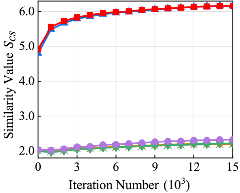
(a) Similarity Value $S_{cs}$

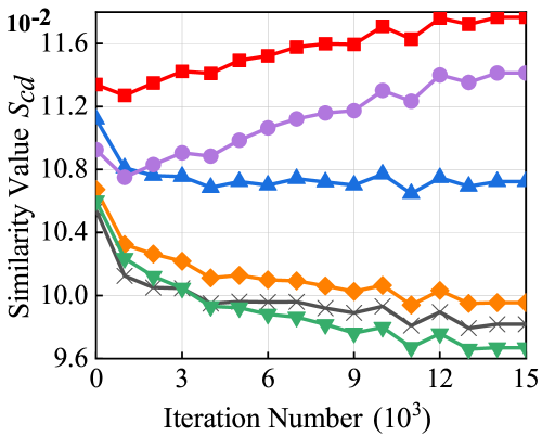
(b) Similarity Value $S_{cd}$

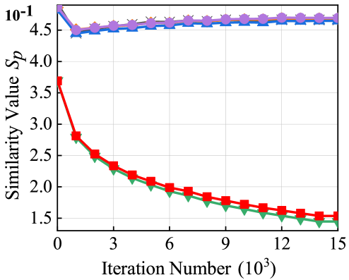
(c) Similarity Value $S_{p}$

Figure 3: Distance analyses of commonality and specificity. Under various combinations of losses, the distances among common features, (a) $S_{cs}$ and (b) $S_{cd}$, and the similarity of the specific parts, (c) $S_{p}$, are computed to illustrate the effectiveness of FS.

On ComCars, as in Table II, we obtain results with similar trends. FSDGs outperform second-best competitors by 3.07% and 4.59%, surpass baselines by 2.58% and 4.91%, and also outperform FGDG (+$\mathcal{L}_{lf}$) by 1.31% and 1.15%, respectively. The best results even surpass the PAN model. Single-backbone models achieve higher performance than dual-backbone models, which can be attributed to the substantial differences between the two domains. It is a challenge to generalize multiple levels of clean knowledge learned by dual backbones to a low-quality single-angle domain S when the model is trained on the high-quality multi-angle domain W.

On Birds-31, as in Table III, our method achieves the highest accuracy, surpassing the second-best method, SAGM, by approximately 9.2%. Under the dual backbone configuration, FSDG outperforms the baseline by 2.32%. On average, across three datasets, FSDG outperforms the second-best approach by up to 6.2%.

TABLE V: Ablation study on the losses (i.e., $\mathcal{L}_{lf}$, $\mathcal{L}_{cs}$, $\mathcal{L}_{p}$, $\mathcal{L}_{cd}$, and $\mathcal{L}_{dec}$). The classification accuracy (%) is presented.

$\mathcal{L}_{lf}$	$\mathcal{L}_{cs}$	$\mathcal{L}_{p}$	$\mathcal{L}_{cd}$	$\mathcal{L}_{dec}$	C→P	P→C	Avg
					56.76	46.53	51.65
✓					60.18	47.13	53.66
✓	✓				61.26	47.76	54.51
✓		✓			60.98	48.07	54.52
✓			✓		60.85	47.52	54.18
✓				✓	60.68	47.51	54.09
✓	✓	✓			61.18	48.55	54.87
✓	✓		✓		61.66	47.77	54.71
✓		✓	✓		60.60	48.50	54.55
	✓	✓	✓		58.96	47.14	53.05
✓	✓	✓	✓		61.77	48.43	55.10
✓	✓	✓	✓	✓	61.84	49.46	55.65

Experiments on various backbones and depths. We conduct experiments on various backbones, including RN-50, RN-101, ViT-Tiny, ViT-Small, ASMLP-Tiny, and ASMLP-Small, as shown in Table IV. Our method exhibits varying degrees of improvement across different architectures, ranging from 1.9 to 4.6%. Upon replacing the backbone with ViT-S, FSDG achieves a performance of 68.26%, surpassing PAN (DA) by 9.1%, showcasing the superiority of Transformer architecture. FS method achieves the highest performance improvement on ASMLP (4.6%). These results validate the robustness of the FSDG method across various backbone architectures.

IV-D Analysis

Ablation study on the losses. We present the outcomes of models optimized under various combinations of losses. As shown in Table V, each loss and their combinations contribute to performance improvement compared to the baseline FGDG model (the first row). The efficacy of the FS approach is substantiated by quantitative assessments of FGDG performance.

Commonality alignment. Fig. 3a and 3b illustrate how the similarities of common features, as depicted in Eq. (4) and (6), evolve throughout the training process under different loss functions. The similarity $S_{cs}$ significantly increases with the introduction of $\mathcal{L}_{cs}$. $\mathcal{L}_{cs}$ forces common parts at different granularities to converge. In other words, features of the common portion can extract the same information for a given sample, ensuring alignment of the shared concepts across various granularities.

$S_{cd}$ signifies the distance among sub-centroids’ commonalities within a particular parent category. Fig. 3b shows that $\mathcal{L}_{cd}$ compels an increase in the similarity among different sub-categories. It can be observed that models lacking alignment tend to perceive common concepts as dissimilar. The network fails to capture the commonalities among sub-classes. The reason behind this is that the network without alignment primarily fits discriminative features at a single granularity level, neglecting the shared characteristics among categories. Undoubtedly, this leads to the introduction of spurious discriminative features and a reduction in generalization ability. Additionally, we observe a similar effect with $\mathcal{L}_{cs}$. The inclusion of $\mathcal{L}_{cs}$ also increases $S_{cd}$. When both losses are included, $S_{cd}$ reaches its optimal value, highlighting the necessity of employing dual common feature alignment constraints. Overall, to a certain extent, $\mathcal{L}_{cs}$ and $\mathcal{L}_{cd}$ have clustered the sub-categories and learned their common features from the perspective of FS.

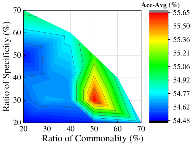
Figure 4: Analyses of the proportions of common, specific, and confounding components.

Specificity alignment. $\mathcal{L}_{p}$ forces the specific segment of different categories to be as far apart as possible. As depicted in Fig. 3c, $\mathcal{L}_{p}$ significantly diminishes the similarity among individuals from different categories, and this gap continues to widen further as the training advances, thereby affirming the efficacy of the devised approach. Moreover, the diminution in specific feature similarity is conducive to amplifying discriminability among category representations, thereby fortifying the capability for fine-grained recognition.

Ratio impact. FSDG reaches its peak when the proportions of commonality, specificity, and confounding are controlled to be 5:3:2, as Fig. 4 shows. As the ratios of commonality and specificity decrease, the performance in FGDG drops to a minimum. Compared to specificity, commonality has a greater impact on generalization. The constraints on the common and specific parts contribute to the improved generalization. Even the lowest performance (54.48%) at the point where common and specific components only account for 20% each is still higher than the case without the $\mathcal{L}_{FS}$ constraint, which is 53.66% in Table I. This is because, in this study, we impose no strict constraints on the confounding part, which means increasing the ratio of the confounding part tends to resemble the original FGDG model. Moreover, performance is degraded when $r^{n}$ is configured as 0, highlighting the necessity of isolating the confounding part from the commonality and specificity at the feature level.

TABLE VI: Classification accuracy (%) and Gpu Hours of various distance metrics. The GPU Hours are tested on conditions: single 3090 GPU, batch size 32, and epoch 1.

Method	C→P	P→C	Avg	Gpu Hours
HSIC	61.10	47.97	54.54	0.34
Euclidean	60.93	47.90	54.41	0.05
Cosine	61.84	49.46	55.65	0.06

TABLE VII: Classification accuracy (%) on various network architectures of the Granularity Transition Layers $T$. BN represents Batch Normalization. Additional configurations for CNN include a stride of 1 and a padding of 1.

Network Architecture	C→P	P→C	Avg
Conv 1$\times$1$\times$ $d$, BN, ReLU, Dropout,	59.10	43.59	51.34
Conv 1$\times$1$\times$ $d$, BN, ReLU, Dropout,
Conv 1$\times$1$\times$256, BN, ReLU,
ShortCut
Conv 1$\times$1$\times$ $d$, BN, ReLU, Dropout,	60.48	46.43	53.45
Conv 1$\times$1$\times$256, BN, ReLU,
ShortCut
Conv 1$\times$1$\times$256, BN, ReLU,	61.50	48.76	55.13
ShortCut
Conv 1$\times$1$\times$ $d$, BN, ReLU, Dropout,	59.05	43.02	51.03
Conv 1$\times$1 $\times$ $d$, BN, ReLU, Dropout,
Conv 1$\times$ 1$\times$ 256, BN, ReLU
Conv 1$\times$1$\times$$d$, BN, ReLU, Dropout,	60.43	46.23	53.33
Conv 1$\times$1$\times$256, BN, ReLU
Conv 1$\times$1$\times$256, BN, ReLU	61.84	49.46	55.65

Experiments on various distance measurements. We conduct experiments with HSIC and Euclidean distance as alternatives of Cosine similarity, as shown in Table VI. From the perspectives of generalization and computational efficiency, we find that the performance achieved by Cosine exceeds that of other methods by approximately 1%, while the computational time is slightly higher than the Euclidean by 0.01 hours, which is acceptable. Besides, Cosine represents the degree of orthogonality between two vectors, which meets our needs. Therefore, we opt to utilize Cosine similarity.

Experiments on various architectures of the Granularity Transition Layer $T$. $T$ refines the globally shared features extracted by backbones, tailoring them specifically to each granularity branch. We configure various structures to construct $T$ with results presented in Table VII. The simplest single-layer CNN achieves the best results. As the number of CNN layers increases, the model’s performance declines, indicating a loss of useful information. Therefore, we choose the single-layer CNN as the Granularity Transition Layer.

TABLE VIII: 4-granularity labels of 8 category examples and the overlap of statistical top concepts between each category and the other 7 categories. The ratio of commonality shows the ratio between the Common and the All.

Category Examples				FGDG	FGDG	FGDG	FGDG	FGDG	FSDG	FSDG	FSDG	FSDG	FSDG
g=0	g=1	g=2	g=3	All	Com.	Spe.	Conf.	Ratio Com.	All	Com.	Spe.	Conf.	Ratio Com.
8	5	3	3	94	36	35	23	38%	61	35	13	13	57%
9	6	3	3	70	24	23	23	34%	62	34	12	16	55%
10	5	3	3	94	39	32	23	41%	70	55	8	7	79%
11	7	3	3	72	27	30	15	38%	65	47	12	6	72%
12	8	3	3	85	29	32	24	34%	58	41	7	10	71%
28	19	12	3	99	45	39	15	45%	60	34	13	13	57%
29	19	12	3	96	37	33	26	39%	64	44	9	11	69%
51	36	19	8	32	18	10	4	56%	32	25	7	0	78%
Average				80	32	29	19	40%	59	40	10	9	68%

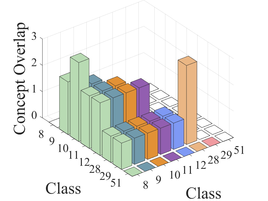
(a) Ground Truth of Concept Overlap

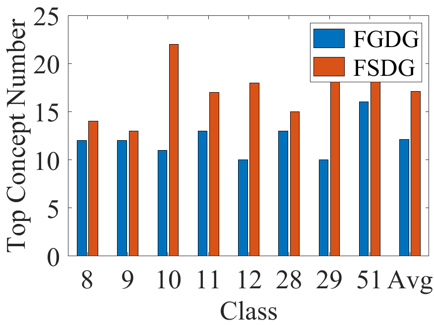
(b) Common

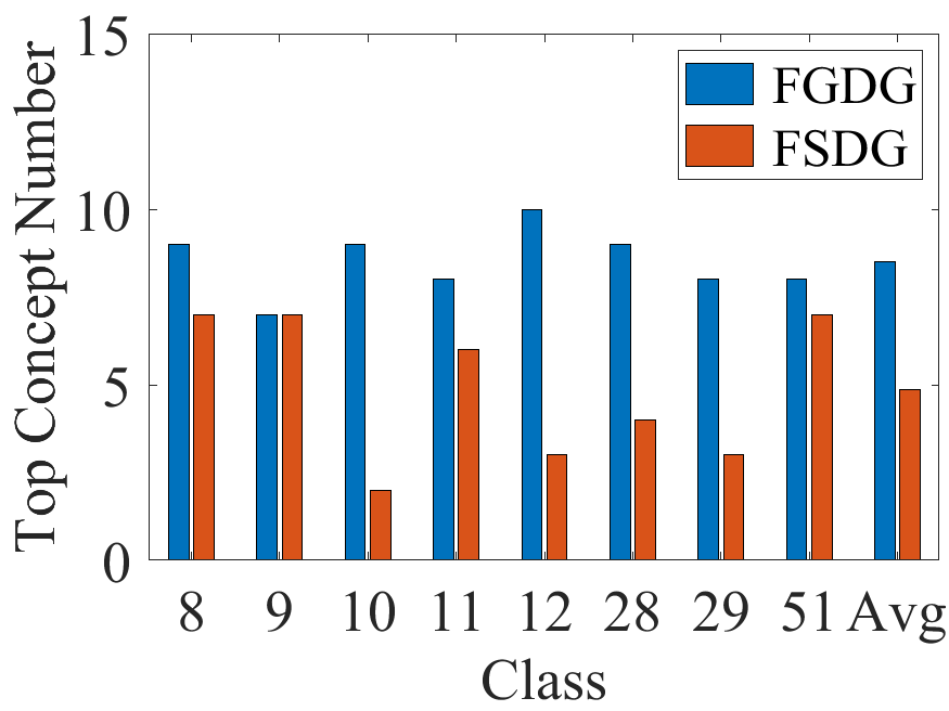
(c) Specific

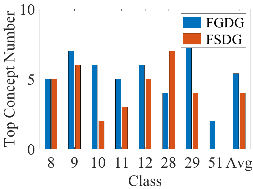
(d) Confounding

Figure 5: Confusion matrix of the ground truth of concept overlaps and the histograms of the most relevant concepts. (b), (c) and (d) plot the number of top concepts belonging to the three segments. Avg shows the average value among 8 categories.

V Explainability Analysis

In this paper, we enhance the FGDG performance through the FS method with the integration of data and knowledge. The demonstrated enhancement primarily manifests in that the common part of the features, decoupled based on channel indices, primarily focuses on the commonalities and representing the invariance between categories, while the specific part focuses on learning discriminative characteristics. In this section, we endeavor to validate that FS increases the explicit concept matching intensity between the shared concepts among categories and the indices of model channels.

We argue that categories that are closer together should activate more identical concepts in the common part, while classes that are farther apart activate fewer shared concepts in this segment. To demonstrate this argument, we randomly select a sequence of classes from the Cub-Paintings dataset, and their corresponding category labels at four granularities are shown in Table VIII. We then define distances based on a multi-granular structure to roughly measure the similarity between fine-grained categories:

$$\mathcal{S}_{class}^{i,j}=d_{i}-\left\|\boldsymbol{c}_{i}-\boldsymbol{c}_{j}\right\|_{0},$$ (14)

where $\boldsymbol{c}_{i}$ is a class vector in which each element represents the class label of the according granularity (e.g., $\boldsymbol{c}_{8}=[8,5,3,3]^{\top}$), and $d_{i}$ reflects the dimension of $\boldsymbol{c}_{i}$, respectively.

$\mathcal{S}_{class}$ is a discrete numerical value, with its maximum determined by the number of granularities in the hierarchical knowledge structure. $\mathcal{S}_{class}$ provides a ranking of the differences between different fine-grained categories. It should be noted that $\mathcal{S}_{class}=0$ does not imply that there is no commonality between two categories but rather indicates low similarity between them within the multi-granular structure. For example, in the Cub-Paintings dataset, all bird species share a consistent body shape, which is a form of commonality. However, this similarity might not be reflected within the current granularity structure. Fig. 5a displays the confusion matrix of $\mathcal{S}_{class}$ between fine-grained category instances as listed in Table VIII. Fig. 5a depicts the ground truth quantifying the difference ranks between categories.

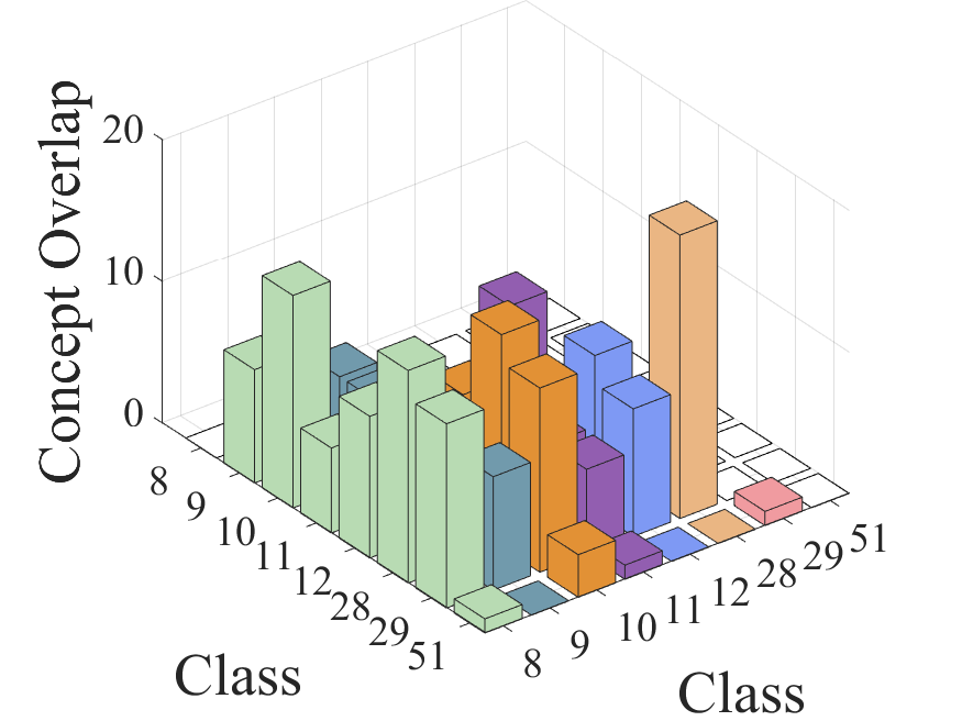
(a) All of FGDG

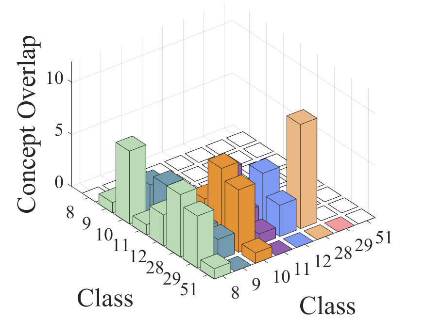
(b) Common of FGDG

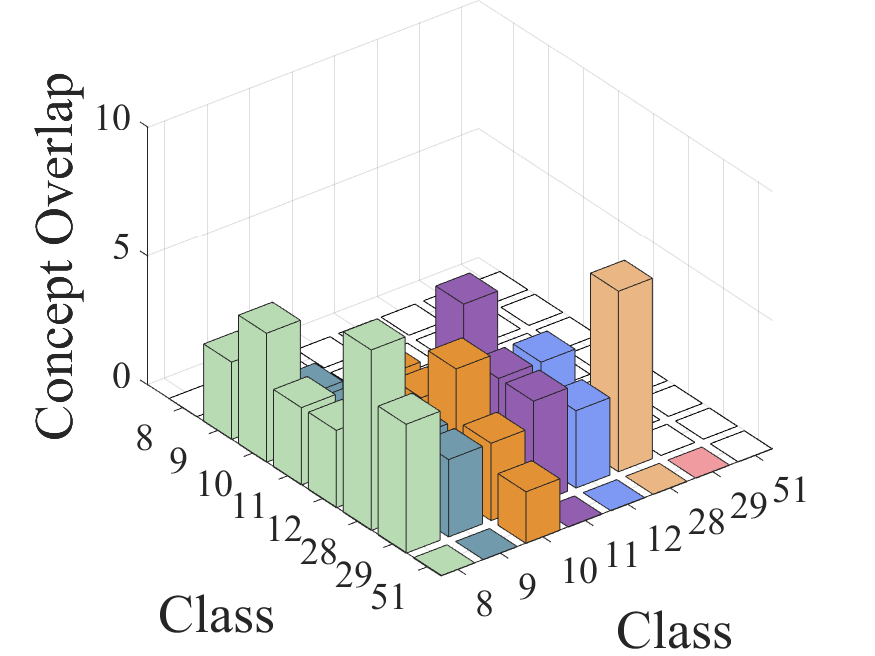
(c) Specific of FGDG

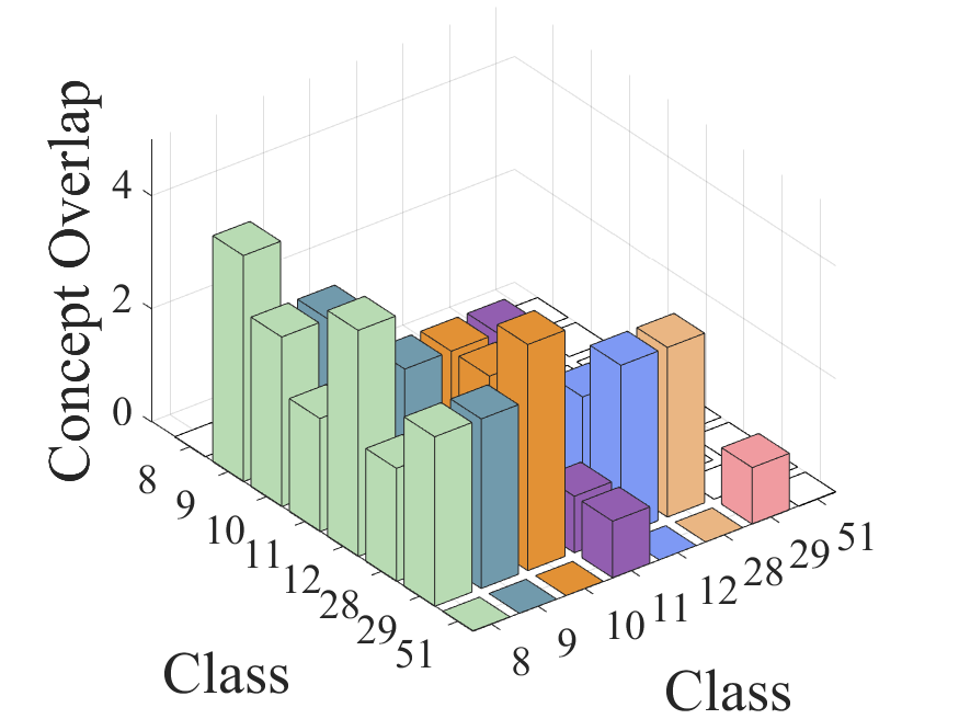
(d) Confounding of FGDG

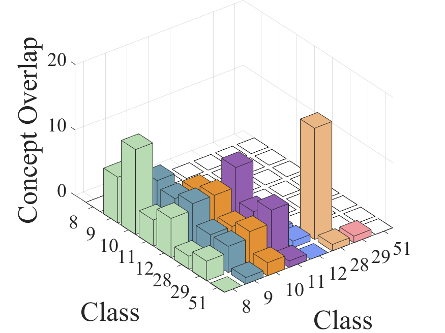
(e) All of FSDG

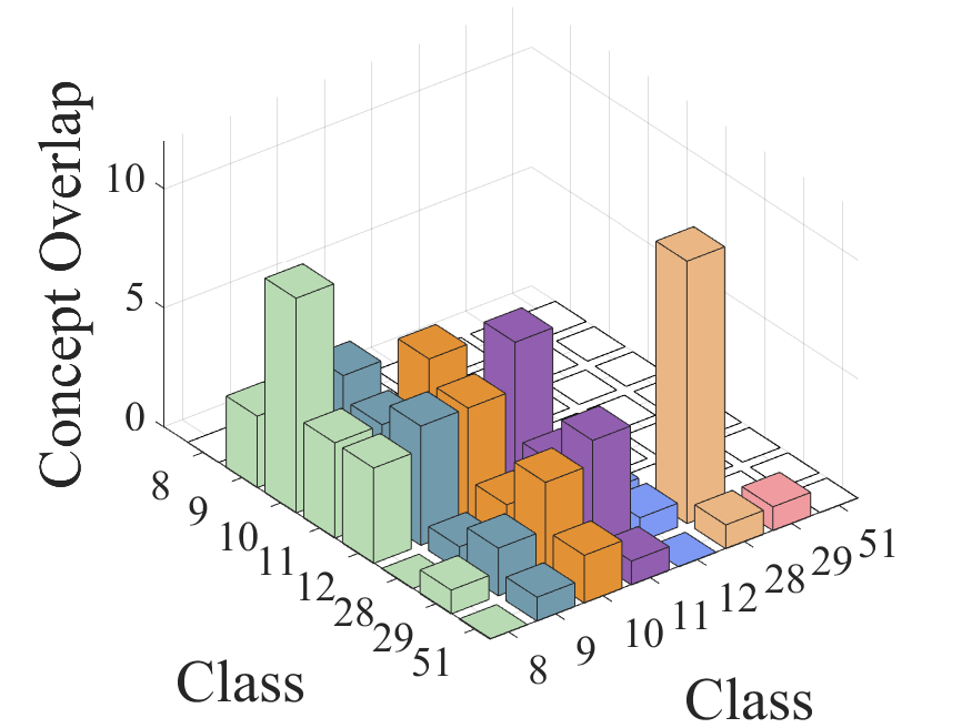
(f) Common of FSDG

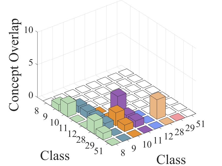
(g) Specific of FSDG

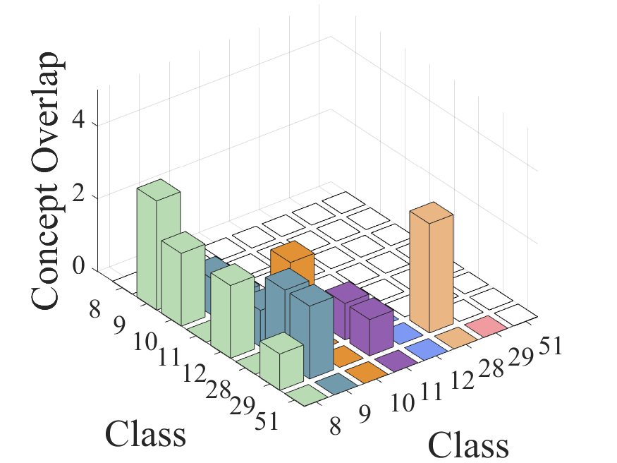
(h) Confounding of FSDG

Figure 6: Confusion matrix of the overlap of relevant concepts between each pair of categories. The first row represents the concept overlaps of the baseline FGDG model, while the second row belongs to the proposed FSDG method. The first column denotes the overlap of all 26 top relevant concepts; the second column denotes those belonging to the common part; the third column denotes the specific part; and the fourth column denotes the confounding part. The computed confusion matrix is symmetric. To enhance visualization, we set the upper triangle of the confusion matrix to zero. The ground truth and the diagonal elements of the confusion matrices are separately plotted in Fig. 5.

We then refine a Concept Relevance Propagation (CRP) technique [18] to acquire the most relevant shared concepts activated by every two categories. Specifically, CRP first records the 40 most relevant samples and their relevance values with respect to each channel of the transition layer $T_{g=0}$. We further refine the CRP by statistically sorting all 256 channels for each class according to their relevance values. As each channel can represent a concept, this statistical outcome achieves relevance ranking for all 256 concepts concerning each class. After that, the top 26 channels and their relevance values of each class are extracted to represent the most relevant concepts. The reason why we choose 26 is that, for a single category, only approximately the top 10% of channels are activated, while the remaining 90% have activation levels less than one-tenth of the maximum activation level.

Fig. 5b-5d illustrate the distributions of the top 26 relevant concepts in three parts. We find that FS leads to an increase in the number of concepts activated in the common region while reducing the activation in the other two regions. For example, among the top 26 concepts in category 10, 22 over 26 concepts are activated at the common part by FS, whereas the baseline FGDG model only has 11. This suggests that, for fine-grained recognition, extracting common concepts is more crucial for generalization as common concepts reflect the invariance between categories.

Intuitively, we argue that closer categories should share more common concepts, meaning that there should be a higher overlap in the most relevant activated channels. We compute the confusion matrix of the overlap of relevant concepts between each pair of category examples, as illustrated in Fig. 6. Compared among Fig. 5a, 6a and 6e, the overall shape of the concept overlap activated by FS closely resembles the ground truth. The FGDG model, without FS, overlooks the relationships between categories, resulting in distant classes having a considerable overlap in activated shared concepts, which is inaccurate. Besides, as shown in Fig. 6b and 6f, FS leads to greater activation of shared concepts in the common part. Besides, the shared concepts between categories are more concentrated in the common partition, which aligns with our initial assumptions and objectives. This also indicates that we, to some extent, pre-define the functionalities of the channels, enhancing the model’s internal transparency and explainability.

When contrasting the distribution of shared concepts in the specific region, as shown in Fig. 6d and Fig. 6h, we observe that FS elicits a sparser distribution of shared concepts. This indicates that this region focuses more on specificities, aligning with the initial assumptions of the model. This phenomenon also occurs in the confounding part. Since we do not impose constraints on the confounding part, a natural discussion arises as to whether applying constraints only to the common and specific parts would increase more activations in the confounding part. In contrast, by analyzing Fig. 5d, Fig. 6d and Fig. 6h, we find that the number of top activations in the confounding part is decreased. All of these results demonstrate that FS directs the model to focus more on capturing the relationships between categories rather than on other spurious correlations, therefore improving generalization.

To quantitatively analyze the matching intensity between shared concepts and channel structure regions, we sum up the number of shared concepts between each category and the other seven categories, as shown in Table VIII. By calculating the proportion of shared concepts within the common region relative to all shared concepts, we find that FS increases the explicit matching intensity between shared concepts and model channels from 40% to 68%. Therefore, our FS approach is indeed effective.

VI Conclusion

In this paper, we assimilate insights from cognitive psychology to advance a feature structuralization framework to tackle the fine-grained domain generalization challenge. FS explicitly embeds structured commonalities and specificities into DL models by integrating data and multi-granularity knowledge. The disentanglement of learned features into common, specific, and confounding segments and their decorrelation, the feature alignment constraints facilitated by three optimization functions, and the prediction calibration term collaboratively contribute to the construction of the FSDG model. Extensive experiments demonstrate a notable enhancement in FGDG performance. Furthermore, the explainability analysis confirms the validity of FS.

Despite FSDG’s systemic efficacy, it brings forth new challenges and prompts intriguing questions. For example, the pre-constructed granularity structure is used to achieve semantic feature alignments. However, some datasets may lack granularity structures, posing challenges to granularity constraints. Notably, one of the prevailing trends in AI research is the pursuit of large-scale datasets, leading to a significant increase in the number of data categories [55]. Such large-scale datasets inherently exhibit hierarchical multi-granularity attributes; for instance, the ImageNet dataset utilizes WordNet for granularity structure delineation [56]. Besides, pioneers have emerged in the research of automatic granularity discovery and construction, such as community discovery [57]. Researchers can upgrade techniques for the automatic construction of granularity based on the commonalities and specificities proposed in this paper. In addition, considering the distance-based nature of FSDG, the incorporation of optimal transport-based training objectives is another promising direction for further boosting performance [58]. This endeavor would help us gain a deeper understanding of the commonalities and specificities among the samples, as well as the gaps between them and their centroids. Another essential future direction deserving of further exploration is the deeper analysis of the explainability. FSDG seeks to render the black-box features of deep learning more transparent, allowing us to identify certain features responsible for handling commonalities and specificities. Thanks to the numerous breakthroughs in techniques witnessed in recent years, we anticipate a surge of innovation in these promising avenues. These further explorations foster the synergistic optimization of feature structuralization. In summary, our work establishes a strong baseline for exploiting FGDG problems, and we believe that the findings presented in this paper warrant further exploration.

References

- [1] J. Zhang, L. Qi, Y. Shi, and Y. Gao, “Exploring flat minima for domain generalization with large learning rates,” IEEE Transactions on Knowledge and Data Engineering, pp. 1–14, 2024.
- [2] J. Wang, C. Lan, C. Liu, Y. Ouyang, T. Qin, W. Lu, Y. Chen, W. Zeng, and P. Yu, “Generalizing to unseen domains: A survey on domain generalization,” IEEE Transactions on Knowledge and Data Engineering, 2022.
- [3] E. Rosenfeld, P. K. Ravikumar, and A. Risteski, “The risks of invariant risk minimization,” in 9th International Conference on Learning Representations, ICLR 2021, Virtual Event, Austria, May 3-7, 2021, 2021.
- [4] H. Wang, K. Kuang, L. Lan, Z. Wang, W. Huang, F. Wu, and W. Yang, “Out-of-distribution generalization with causal feature separation,” IEEE Transactions on Knowledge and Data Engineering, vol. 36, no. 4, pp. 1758–1772, 2024.
- [5] K. Zhou, Z. Liu, Y. Qiao, T. Xiang, and C. C. Loy, “Domain generalization: A survey,” IEEE Transactions on Pattern Analysis and Machine Intelligence, 2022.
- [6] X.-S. Wei, Y.-Z. Song, O. M. Aodha, J. Wu, Y. Peng, J. Tang, J. Yang, and S. Belongie, “Fine-grained image analysis with deep learning: A survey,” IEEE Transactions on Pattern Analysis and Machine Intelligence, vol. 44, no. 12, pp. 8927–8948, 2022.
- [7] S. Wang, X. Chen, Y. Wang, M. Long, and J. Wang, “Progressive adversarial networks for fine-grained domain adaptation,” in Proceedings of the IEEE/CVF conference on computer vision and pattern recognition, 2020, pp. 9213–9222.
- [8] S. Mao and S. Zhang, “Robust fine-grained visual recognition with neighbor-attention label correction,” IEEE Transactions on Image Processing, vol. 33, pp. 2614–2626, 2024.
- [9] E. Rosch and C. B. Mervis, “Family resemblances: Studies in the internal structure of categories,” Cognitive Psychology, vol. 7, pp. 573–605, 1975.
- [10] A. Treisman and G. A. Gelade, “A feature-integration theory of attention,” Cognitive Psychology, vol. 12, pp. 97–136, 1980.
- [11] J. A. Brooks and J. B. Freeman, “Conceptual knowledge predicts the representational structure of facial emotion perception,” Nature Human Behaviour, vol. 2, pp. 581 – 591, 2018.
- [12] Y. he Pan, “On visual knowledge,” Frontiers of Information Technology & Electronic Engineering, vol. 20, pp. 1021 – 1025, 2019.
- [13] Y. Sun, Y. Zhu, Y. Zhang, P. Zheng, X. Qiu, C. Zhang, and Y. Wei, “Dynamic metric learning: Towards a scalable metric space to accommodate multiple semantic scales,” in Proceedings of the IEEE/CVF Conference on Computer Vision and Pattern Recognition, 2021, pp. 5393–5402.
- [14] W. Wang, Y. Yang, and Y. Pan, “Visual knowledge in the big model era: Retrospect and prospect,” arXiv e-prints, pp. arXiv–2404, 2024.
- [15] F. Locatello, S. Bauer, M. Lucic, G. Raetsch, S. Gelly, B. Schölkopf, and O. Bachem, “Challenging common assumptions in the unsupervised learning of disentangled representations,” in international conference on machine learning. PMLR, 2019, pp. 4114–4124.
- [16] B. Zhou, D. Bau, A. Oliva, and A. Torralba, “Interpreting deep visual representations via network dissection,” IEEE Transactions on Pattern Analysis and Machine Intelligence, vol. 41, pp. 2131–2145, 2019.
- [17] H. Liu, R. Wang, S. Shan, and X. Chen, “What is tabby? interpretable model decisions by learning attribute-based classification criteria,” IEEE transactions on pattern analysis and machine intelligence, 2019.
- [18] R. Achtibat, M. Dreyer, I. Eisenbraun, S. Bosse, T. Wiegand, W. Samek, and S. Lapuschkin, “From attribution maps to human-understandable explanations through concept relevance propagation,” Nature Machine Intelligence, vol. 5, no. 9, pp. 1006–1019, 2023.
- [19] Y. Gandelsman, A. A. Efros, and J. Steinhardt, “Interpreting clip’s image representation via text-based decomposition,” in The Twelfth International Conference on Learning Representations, 2024.
- [20] J. S. Yoon, K. Oh, Y. Shin, M. A. Mazurowski, and H.-I. Suk, “Domain generalization for medical image analysis: A survey,” arXiv preprint arXiv:2310.08598, 2023.
- [21] K. Muandet, D. Balduzzi, and B. Schölkopf, “Domain generalization via invariant feature representation,” in International conference on machine learning. PMLR, 2013, pp. 10–18.
- [22] B. Sun and K. Saenko, “Deep coral: Correlation alignment for deep domain adaptation,” in Computer Vision–ECCV 2016 Workshops: Amsterdam, The Netherlands, October 8-10 and 15-16, 2016, Proceedings, Part III 14. Springer, 2016, pp. 443–450.
- [23] K. Zhou, Y. Yang, Y. Qiao, and T. Xiang, “Domain generalization with mixstyle,” in International Conference on Learning Representations, 2021.
- [24] S. Yan, H. Song, N. Li, L. Zou, and L. Ren, “Improve unsupervised domain adaptation with mixup training,” arXiv preprint arXiv:2001.00677, 2020.
- [25] P. Wang, Z. Zhang, Z. Lei, and L. Zhang, “Sharpness-aware gradient matching for domain generalization,” in Proceedings of the IEEE/CVF Conference on Computer Vision and Pattern Recognition, 2023, pp. 3769–3778.
- [26] M. Zhang, H. Marklund, N. Dhawan, A. Gupta, S. Levine, and C. Finn, “Adaptive risk minimization: Learning to adapt to domain shift,” Advances in Neural Information Processing Systems, vol. 34, pp. 23 664–23 678, 2021.
- [27] D. Li, Y. Yang, Y.-Z. Song, and T. Hospedales, “Learning to generalize: Meta-learning for domain generalization,” in Proceedings of the AAAI conference on artificial intelligence, vol. 32, no. 1, 2018.
- [28] M. Ilse, J. M. Tomczak, C. Louizos, and M. Welling, “Diva: Domain invariant variational autoencoders,” in Medical Imaging with Deep Learning. PMLR, 2020, pp. 322–348.
- [29] L. Chen, Y. Zhang, Y. Song, A. van den Hengel, and L. Liu, “Domain generalization via rationale invariance,” in Proceedings of the IEEE/CVF International Conference on Computer Vision, 2023, pp. 1751–1760.
- [30] F. Qiao, L. Zhao, and X. Peng, “Learning to learn single domain generalization,” in 2020 IEEE/CVF Conference on Computer Vision and Pattern Recognition (CVPR), Jun 2020.
- [31] K. Zhou, Y. Yang, T. M. Hospedales, and T. Xiang, “Deep domain-adversarial image generation for domain generalisation,” in The Thirty-Fourth AAAI Conference on Artificial Intelligence, 2020, pp. 13 025–13 032.
- [32] G. Wang, H. Han, S. Shan, and X. Chen, “Cross-domain face presentation attack detection via multi-domain disentangled representation learning,” 2020 IEEE/CVF Conference on Computer Vision and Pattern Recognition, pp. 6677–6686, 2020.
- [33] V. Piratla, P. Netrapalli, and S. Sarawagi, “Efficient domain generalization via common-specific low-rank decomposition,” in International Conference on Machine Learning. PMLR, 2020, pp. 7728–7738.
- [34] H. Chen, H. Zhang, C. Liu, J. An, Z. Gao, and J. Qiu, “Fet-fgvc: Feature-enhanced transformer for fine-grained visual classification,” Pattern Recognition, vol. 149, p. 110265, 2024.
- [35] X. Zheng, L. Qi, Y. Ren, and X. Lu, “Fine-grained visual categorization by localizing object parts with single image,” IEEE Transactions on Multimedia, vol. 23, pp. 1187–1199, 2021.
- [36] H. Sun, X. He, and Y. Peng, “Sim-trans: Structure information modeling transformer for fine-grained visual categorization,” in Proceedings of the 30th ACM International Conference on Multimedia, 2022, pp. 5853–5861.
- [37] J. Li, L. Yang, Q. Wang, and Q. Hu, “Wdan: A weighted discriminative adversarial network with dual classifiers for fine-grained open-set domain adaptation,” IEEE Transactions on Circuits and Systems for Video Technology, vol. 33, pp. 5133–5147, 2023.
- [38] M. G. Preti and D. Van De Ville, “Decoupling of brain function from structure reveals regional behavioral specialization in humans,” Nature communications, vol. 10, no. 1, p. 4747, 2019.
- [39] A. Gretton, K. Fukumizu, C. Teo, L. Song, B. Schölkopf, and A. Smola, “A kernel statistical test of independence,” Advances in neural information processing systems, vol. 20, 2007.
- [40] P.-E. Danielsson, “Euclidean distance mapping,” Computer Graphics and image processing, vol. 14, no. 3, pp. 227–248, 1980.
- [41] E. Tzeng, J. Hoffman, T. Darrell, and K. Saenko, “Simultaneous deep transfer across domains and tasks,” in Proceedings of the IEEE international conference on computer vision, 2015, pp. 4068–4076.
- [42] C. Wah, S. Branson, P. Welinder, P. Perona, and S. Belongie, “The caltech-ucsd birds-200-2011 dataset,” 2011.
- [43] L. Yang, P. Luo, C. C. Loy, and X. Tang, “A large-scale car dataset for fine-grained categorization and verification,” in 2015 IEEE Conference on Computer Vision and Pattern Recognition CVPR, Jun 2015.
- [44] G. Van Horn, S. Branson, R. Farrell, S. Haber, J. Barry, P. Ipeirotis, P. Perona, and S. Belongie, “Building a bird recognition app and large scale dataset with citizen scientists: The fine print in fine-grained dataset collection,” in Proceedings of the IEEE conference on computer vision and pattern recognition, 2015, pp. 595–604.
- [45] G. Van Horn, O. Mac Aodha, Y. Song, Y. Cui, C. Sun, A. Shepard, H. Adam, P. Perona, and S. Belongie, “The inaturalist species classification and detection dataset,” in Proceedings of the IEEE conference on computer vision and pattern recognition, 2018, pp. 8769–8778.
- [46] V. Vapnik, The nature of statistical learning theory. Springer science & business media, 1999.
- [47] Y. Ganin, E. Ustinova, H. Ajakan, P. Germain, H. Larochelle, F. Laviolette, M. March, and V. Lempitsky, “Domain-adversarial training of neural networks,” Journal of machine learning research, vol. 17, no. 59, pp. 1–35, 2016.
- [48] S. Sagawa, P. W. Koh, T. B. Hashimoto, and P. Liang, “Distributionally robust neural networks for group shifts: On the importance of regularization for worst-case generalization,” in International Conference on Learning Representations, 2020.
- [49] H. Nam, H. Lee, J. Park, W. Yoon, and D. Yoo, “Reducing domain gap by reducing style bias,” in Proceedings of the IEEE/CVF Conference on Computer Vision and Pattern Recognition, 2021, pp. 8690–8699.
- [50] J. Cha, K. Lee, S. Park, and S. Chun, “Domain generalization by mutual-information regularization with pre-trained models,” in European Conference on Computer Vision. Springer, 2022, pp. 440–457.
- [51] K. He, X. Zhang, S. Ren, and J. Sun, “Deep residual learning for image recognition,” in Proceedings of the IEEE conference on computer vision and pattern recognition, 2016, pp. 770–778.
- [52] A. Dosovitskiy, L. Beyer, A. Kolesnikov, D. Weissenborn, X. Zhai, T. Unterthiner, M. Dehghani, M. Minderer, G. Heigold, S. Gelly, J. Uszkoreit, and N. Houlsby, “An image is worth 16x16 words: Transformers for image recognition at scale,” in International Conference on Learning Representations, 2021.
- [53] D. Lian, Z. Yu, X. Sun, and S. Gao, “AS-MLP: an axial shifted MLP architecture for vision,” in The Tenth International Conference on Learning Representations, Virtual Event, April 25-29, 2022, 2022.
- [54] I. Gulrajani and D. Lopez-Paz, “In search of lost domain generalization,” in 9th International Conference on Learning Representations, ICLR 2021, Virtual Event, Austria, May 3-7, 2021, 2021.
- [55] H. Zhao, Q. Hu, P. Zhu, Y. Wang, and P. Wang, “A recursive regularization based feature selection framework for hierarchical classification,” IEEE Transactions on Knowledge and Data Engineering, vol. 33, no. 7, pp. 2833–2846, 2019.
- [56] O. Russakovsky, J. Deng, H. Su, J. Krause, S. Satheesh, S. Ma, Z. Huang, A. Karpathy, A. Khosla, M. Bernstein et al., “Imagenet large scale visual recognition challenge,” International journal of computer vision, vol. 115, pp. 211–252, 2015.
- [57] S. Qiao, N. Han, Y. Gao, R.-H. Li, J. Huang, J. Guo, L. A. Gutierrez, and X. Wu, “A fast parallel community discovery model on complex networks through approximate optimization,” IEEE Transactions on Knowledge and Data Engineering, vol. 30, no. 9, pp. 1638–1651, 2018.
- [58] M. Cuturi, “Sinkhorn distances: Lightspeed computation of optimal transport,” Advances in neural information processing systems, vol. 26, 2013.