Diffusion Gaussian Mixture Audio Denoise

Abstract

Recent diffusion models have achieved promising performances in audio-denoising tasks. The unique property of the reverse process could recover clean signals. However, the distribution of real-world noises does not comply with a single Gaussian distribution and is even unknown. The sampling of Gaussian noise conditions limits its application scenarios. To overcome these challenges, we propose a DiffGMM model, a denoising model based on the diffusion and Gaussian mixture models. We employ the reverse process to estimate parameters for the Gaussian mixture model. Given a noisy audio signal, we first apply a 1D-U-Net to extract features and train linear layers to estimate parameters for the Gaussian mixture model, and we approximate the real noise distributions. The noisy signal is continuously subtracted from the estimated noise to output clean audio signals. Extensive experimental results demonstrate that the proposed DiffGMM model achieves state-of-the-art performance.

1 Introduction

Audio signals are the main source of biological information transmission in nature, and various organisms interact through a wide range of sounds [1], such as recording recognition [2], audio-to-text capabilities in social media [3], and assistive hearing [4]. However, due to the existence of noise in the actual environment, the original audio becomes impure during the transmission of the audio signal. Audio denoising can significantly improve the quality of polluted audio and the accuracy of speech recognition. Conventional denoising methods have a significant effect on the suppression of stationary noise, but for non-stationary noise, it often cannot achieve a good noise reduction effect [5]. Deep neural networks (DNNs) based methods commonly take a set of frequency coefficients of a short time period of the noisy signal and use paired data of noisy sounds and the corresponding clean sounds to train their denoising model [6, 7].

Generative models include generative adversarial networks (GAN) [8], variational autoencoders (VAEs) [9], flow-based neural networks [10], and diffusion models [11]. The diffusion model is a deep generative model that is based on two stages: a forward diffusion stage and a reverse diffusion stage. In the forward diffusion process, a Markov chain with a diffusion step (the current state is only related to the state of the previous moment) slowly adds random noise to the real data until the image becomes completely random noise. In the reverse process, data is recovered from Gaussian noise by using a series of Markov chains to gradually remove the predicted noise at each time step. In this paper, we use the reverse process from the diffusion model for audio noise reduction problem.

Diffusion probability models are a class of generation models that have shown excellent performance for image generation [12], audio synthesis [13], and audio denoising [14, 15]. However, in the real condition, the distribution of noises does not comply with a single Gaussian distribution and is even unknown. One single Gaussian distribution is not enough to represent the original noise distribution. The sampling of Gaussian noise conditions limits its application scenarios. Addressing non-Gaussian noise is another challenge in diffusion models. We try to estimate the distributions of audio in the reverse process instead of the isotropic Gaussian noise. Gaussian mixture models can use these estimated parameters to generate approximate noise. The noisy signal is continuously subtracted from the estimated noise to output clean audio signals. In this paper, we propose a DiffGMM model, a denoising model based on the diffusion and Gaussian mixture models. Our contributions are three-fold:

• We develop a diffusion Gaussian mixture model (DiffGMM), which applies the reverse process of the diffusion model to estimate parameters for the Gaussian mixture model.

• Given a noisy audio signal, we first use a 1D-U-Net to extract features and train linear layers to estimate parameters for the Gaussian mixture model. We then approximate any arbitrary distributions of noise. By constantly subtracting the approximation noise from the original noisy audio, we can distill a clean audio signal.

• Extensive experiments on two benchmark datasets reveal that DiffGMM outperforms state-of-the-art methods.

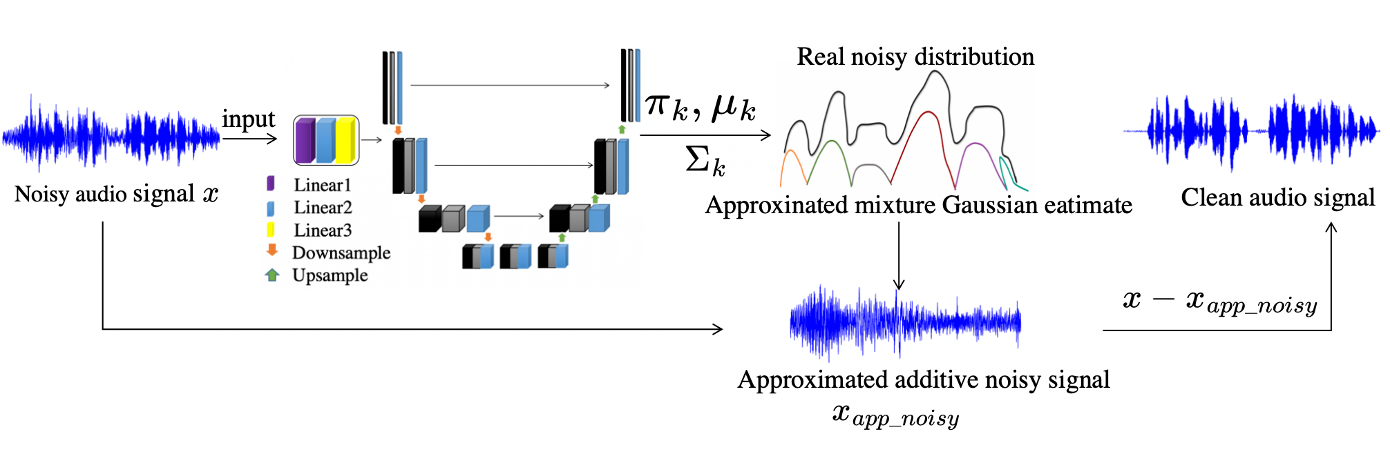
Figure 1: Flowchart of our diffusion Gaussian mixture (DiffGMM) model. We first utilize a 1D-U-Net to estimate the parameters $\pi_{k},\mu_{k}$ and $\Sigma_{k}$ of GMM. We then approximate the additive noise distribution ($x_{app\_noisy}$) using GMM. The real noise is one representation to ease understanding of the GMM approximation. Finally, we continuously utilize the noisy audio signal to subtract the estimated additive noisy signal to distill a clean audio signal.

2 Methods

2.1 Problem

A noisy audio signal $x$ can be typically expressed as:

$$x=y+\varepsilon$$ (1)

where $y$ and $\varepsilon$ denote clean audio and additive noisy signals. Given a clean audio signal and noisy audio signal $\{y_{i}\}_{i=1}^{N}$ and $\{x_{i}\}_{i=1}^{N}$, the goal of audio denoising is to extract the clean audio component $\{y_{i}\}_{i=1}^{N}$ from the noisy audio signal $\{x_{i}\}_{i=1}^{N}$ by learning a mapping $\mathcal{M}$, then minimize the approximation error between the denoised audio $\{\mathcal{M}(x_{i})\}_{i=1}^{N}$ and clean audio $\{y_{i}\}_{i=1}^{N}$. In our DiffGMM model, we use the noisy audio signal $\{x_{i}\}_{i=1}^{N}$ to continuously subtract the approximation noise to reconstruct clean signals.

2.2 Motivation

The diffusion model has an inherent disadvantage, $i.e.,$ a large number of sampling steps and a long sampling time because the diffusion step using Markov nuclei has only a small perturbation, but results in a large amount of diffusion. The operable model requires the same number of steps in the inference process. Therefore, it takes thousands of steps to sample the random noise until it finally changes to high-quality data similar to the prior data. At the same time, the diffusion model also limits the study of arbitrary distribution noise. Our DiffGMM model ignores the unnecessary forward process, given noisy audios are provided. We employ the reverse process to estimate parameters for the Gaussian mixture model to approximate the real noise distribution.

2.3 Preliminary

2.3.1 Reverse Process.

The reverse process is a denoising process in which $q(x_{t-1}|x_{t})$ is predicted by a neural network $p_{\theta}(x_{t-1}|x_{t})$. The reverse process converts $x_{T}$ to $x_{t}$, where $t$ represents the time $t$, and $T$ is the number of steps. We will continuously remove $T$ steps of Gaussian noise using Eq. (2).

$$p_{\theta}(x_{0:T}):=p(x_{T})\prod^{T}_{t=1}p_{\theta}(x_{t-1}|x_{t})$$ (2)

$$p_{\theta}(x_{t-1}|x_{t}):=N(x_{t-1}:\mu_{\theta}(x_{t},t),\Sigma_{\theta}(x_{t},t))$$ (3)

We cannot derive $x_{t-1}$ directly from $x_{t}$ because of insufficient conditions. We add condition $x_{0}$ to get $q(x_{t-1}|x_{t},x_{0})$, which is easy to predict $x_{t-1}$. We then get the Bayesian formula for $q(x_{t-1}|x_{t},x_{0})$ as:

$$q(x_{t-1}|x_{t},x_{0})=\frac{q(x_{t}|x_{t-1},x_{0})q(x_{t-1}|x_{0})}{q(x_{t}|x_{0})}$$ (4)

By introducing negative logarithmic likelihood $-log(p_{\theta}(x_{0}))$, we hope that the parameter $\theta$ of the neural network can make the probability of generating Eq. (2) as large as possible. However, $p_{\theta}(x_{0})$ depends on all the steps up to $x_{0}$, and $p_{\theta}(x_{0})$ is not easy to solve. The solution is to calculate the variation and lower bounds of the target:

$$\begin{split}&D_{KL}(q(x_{T}|x_{0}||p(x_{T})))\\ &+\sum^{T}_{t=2}D_{KL}(q(x_{t-1}|x_{t},x_{0})||p_{\theta}(x_{t-1}|x_{t}))-log(p_{\theta}(x_{0}|x_{1}))\end{split}$$

From the KL divergence, we can find $q(x_{t-1}|x_{t},x_{0})$ in terms of $x_{0}$:

$$q(x_{t-1}|x_{t},x_{0})=N(x_{t-1}:\widetilde{{\mu_{t}}}(x_{t},x_{0}),\widetilde{\beta}_{t}{I})$$ (5)

where $\widetilde{\mu_{t}}(x_{t},x_{0})$ is the true value of the mean in the reverse process, $\widetilde{\beta}_{t}$ is the true value of the difference in the reverse process, $\widetilde{\beta}_{t}:=\frac{1-\widetilde{\alpha}_{t-1}}{1-\widetilde{\alpha_{t}}}{\beta_{t}}$ is fixed to a constant.

2.3.2 Gaussian mixture model

Gaussian mixture model is used to combine multiple Gaussian distributions into a global distribution:

$$p(x_{i}|\theta_{k})=\sum^{K}_{k=1}\pi_{k}N(x_{i}|\mu_{k},\Sigma_{k}),i=1,...,N$$ (6)

where, $K$ is the number of Gaussian distributions, $\theta_{k}={(\mu_{k},\Sigma_{k},\pi_{k})}$ is the collection of all unknown parameters, $\pi_{k}$ is the mixing proportions, $\mu_{k}$ is the mean vector and $\Sigma_{k}$ is the covariance matrix. The mixture coefficient $\pi_{k}$ satisfies: $\sum^{K}_{k=1}\pi_{k}=1,0\leq\pi_{k}\leq 1$. Therefore, we aim to estimate the parameters $\pi_{k},\mu_{k},\Sigma_{k}$ for GMM in our model.

2.4 Methodology

We assume different signals have independent and different distributions. By maximizing the product of probability density functions for all samples, we can optimize Linear layers to estimate GMM parameters $(\mu_{k},\Sigma_{k}$, and $\pi_{k})$. In other words, maximizing the product of the probability density functions of all samples is equivalent to maximizing the sum of the logarithmic probability density functions of all samples. Given $N$ observation $\{x_{n}\}_{n=1}^{N}$, we take advantages of the logarithm and convert multiplication to addition. The log-likelihood function is:

$$ln\ q(X;\pi_{1:K},\mu_{1:K},\Sigma_{1:K})=\sum^{N}_{n=1}ln(p(x_{n}|\theta_{k})).$$ (7)

Considering arbitrary distribution $q(z)$ over the latent variables, the following decomposition always holds:

$$lnp(x|\theta)=\pounds(q,\theta)+KL(q||p)$$ (8)

where

Therefore, we could use the GMM model to estimate the arbitrary distribution of audio signals. We first created an empty estimated noisy signal with the same dimension as the noisy signal and then trained the neural network $f_{\theta}$ to fit the noisy signal. Our goal is to solve the minimization problem:

$$min_{\theta}||f_{\theta}(x)-(x-y)||$$ (10)

where $x$ is the input noisy signal, $y$ is the clean signal. $x-y$ is the true noisy signal and $f_{\theta}(x)$ is the estimated noisy signal. In each iteration $i$ of training, $f_{i}$ represents the current network. By subtracting the estimated noisy signal $f_{\theta}$ from input noisy signal $x$, a partially denoised signal $f_{i}(x)$ is generated.

$$f_{i}(x)=x-f_{\theta}(x)$$ (11)

With the increasing number of iterations, $f_{i}$ output is more expressive, and the proportion of noisy signal in $f_{i}(x)$ is getting smaller and smaller. Each iteration consists of the following steps in Alg. 1.

Algorithm 1 Gaussian mixture model parameters estimation process. $I$ is the number of iterations

1:  Input: original audio: $x$

2:  Output: Gaussian parameters: $\pi_{k},\mu_{k},\Sigma_{k}$

3:  for $i=1$ to $I$ do

4:     Generate initial denoising audios by 1-D U-Net.

5:     $\pi_{k},\mu_{k},\Sigma_{k}$ by training the linear layers

6:     $f_{i}\longleftarrow{f_{i-1}}$ // pass one training iteration on $f_{i-1}$starting with $\theta=\theta_{i-1}$ obtaining $f_{i}$

7:     Generate denoised signal $f_{i}(x)$ by Eq. (11)

8:     Minimize objective optimization function by Eq. (10)

9:     Update parameters $\pi_{k},\mu_{k},\Sigma_{k}$

10:  end for

In our proposed DiffGMM model, we take the estimated noise $p(x_{i})$ in the Gaussian mixture model as the complete Gaussian noise in the diffusion process. In the new reverse process, we apply the Gaussian Markov chain model still $q(x_{t}|x_{0})$. We use a 1D-U-Net to extract features and train linear layers to estimate parameters for the Gaussian mixture model. According to Eq. (3), estimating noise $p(x_{i})$, whose variance is $\Sigma_{k}$ , starts from $x_{T}$ to predict $x_{t-1}$. We can then approximate the real noise distribution $p_{DiffGMM}(x_{t-1}|x_{t})$. The noisy signal is continuously subtracted from the estimated noise to output clean audio signals: $p_{DiffGMM}(x_{t-1}|x_{t})=N(x_{t}|\mu,\Sigma)-\sum^{K}_{k=1}\pi_{k}N(x_{t-1}|\mu_{k},\Sigma_{k})$.

2.4.1 Loss Function

In our DiffGMM model, we use the L1 loss function to train the 1D-U-Net model as follows.

$$J(\theta)=\dfrac{1}{2}\sum_{i=1}^{m}(f_{\theta}(x_{i})-y_{i})^{2},\quad f(\theta)=\sum_{j=0}^{n}\theta_{j}x_{j}$$ (12)

where $f(x)$ is the function to be fitted, $z$ is the number of records in the training set, $j$ is the number of parameters, and $\theta$ is the parameter to be iteratively solved.

We can define the evidence lower bound (ELBO) loss as the training objective of the reverse process. Based on Eq. (8), we rewrite the optimization likelihood:

$$ELBO =-E_{q}(D_{KL}(q(x_{T}|x_{0})||p_{GMM\_diff}(x_{T}|x_{i}))$$ (13)

$$+\sum^{T}_{t=2}D_{KL}(q(x_{t-1}|x_{t})||p_{\theta}(x_{t-1}|x_{t}))-logp_{\theta}(x_{0}|x_{1}))$$

The first term can be ignored because there is no parameter $\theta$ in this term. The third term is a known constant term, and we need to estimate only the second term:

$$L_{t-1}=\sum^{T}_{t=2}D_{KL}(q(x_{t-1}|x_{t})||p_{\theta}(x_{t-1}|x_{t}))$$ (14)

Therefore, we have:

$$L_{t-1}=C+E_{x_{0},x_{i},\epsilon}[\frac{1}{2\Sigma_{k}^{2}}||\frac{1}{\mu_{k}}(x_{t}(x_{0},\epsilon)-{\frac{\Sigma_{k}}{\mu_{k}}})-\mu_{\theta}(x_{t}(x_{0},\epsilon)||^{2}]$$ (15)

where $C$ is a constant independent of $\theta$. By parameterizing Eq. (15) simplifies to:

$$\begin{split}L_{simple}(\theta)&:=E_{t,x_{0},x_{i},\epsilon}[||\epsilon-\epsilon_{\theta}(\mu_{k},x_{0})+(1-\mu_{k})\epsilon),t||^{2}]\end{split}$$ (16)

where $\epsilon$ is the noise in $x_{t}$.

DiffGMM overall algorithm Considering all steps in Sec. 2.4, the scheme of our proposed DiffGMM model is shown in Fig. 1, and the overall algorithm is presented in Alg. 2. In Alg. 1, we get the optimal number of mixture Gaussian models of $K$ as 5, where $x_{app\_noisy}$ denotes the estimated noisy signal.

Algorithm 2 GMM and diffusion Audio Denoising (DiffGMM)

1:  Input: $K=5(k=1,\ldots,5)$, $\pi_{k},\mu_{k},\Sigma_{k}\longleftarrow{\text{1D-U-Net}}$

2:  for $i=1$ to $N$ do

3:     Approximation noise $x_{app\_noisy}\longleftarrow{GMM}$

4:     Denoised audio signal $y_{i}\longleftarrow{x_{i}-x_{app\_noisy}}$

5:  end for

6:  Output: Denoised audio signal $y$

3 Experiments

3.1 Datasets

We evaluate our model using two benchmark datasets: VoiceBank-Demand [16] and BirdSoundsDenoising datasets [7]. VoiceBank-Demand dataset. In this widely used noisy speech database, 251 clean speech datasets are selected from the Voice Bank corpus, including training set 252 of 11572 utterances and a test set of 872 utterances. BirdSoundsDenoising dataset. This bird sounds dataset contains many natural noises, including wind, waterfall, etc. The dataset is a large-scale dataset of bird sounds collected containing 10,000/1,400/2,720 in training, validation, and testing, respectively. We also choose some commonly used metrics to evaluate the enhanced speech quality [17, 18], i.e., PESQ, STOI, CSIG, CBAK, and COVL. The higher these evaluation metrics are, the better the model performs. Demo samples are available at https://giffgmm.github.io.

Table 1: Comparison results on the VoiceBank-DEMAND dataset. ``-" means not applicable.

Methods	Domain	PESQ	STOI	CSIG	CBAK	COVL
DiffuSE(Base) [14]	T	2.41	-	3.61	2.81	2.99
CDiffuSE(Base) [19]	T	2.44	-	3.66	2.83	3.03
PGGAN [20]	T	2.81	0.944	3.99	3.59	3.36
DCCRGAN [21]	TF	2.82	0.949	4.01	3.48	3.40
PHASEN [22]	TF	2.99	$-$	4.18	3.45	3.50
MetricGAN+ [23]	TF	3.15	0.927	4.14	3.12	3.52
PFPL [24]	T	3.15	0.950	4.18	3.60	3.67
MANNER [25]	T	3.21	0.950	4.53	3.65	3.91
TSTNN [26]	T	2.96	0.950	4.33	3.53	3.67
DPT-FSNet [27]	TF	3.33	0.960	4.58	3.72	4.00
CMGAN [28]	TF	3.41	0.960	4.63	3.94	4.12
DiffGMM	T	3.48	0.960	4.72	4.12	4.34

Table 2: Ablation study results

Model	PESQ
GMM-only	3.02
Diffusion-only	2.79
Full Model	3.48

3.2 Implementation details

Training: The complete training pipeline is shown in Alg. 2. We implement our model with a Tesla P100 GPU to speed up the computation. We used the Adam optimizer for neural networks to update the network parameters $\pi_{k}$, $\mu_{k}$, $\Sigma_{k}$. During the training, the input data tensor is $8\times 1\times 5$ (k=5), and the output data tensor from the estimated GMM model is $8\times 1\times 173568$. The 1D-U-Net has 6 layers, each with 60 filters. We use the Adam optimizer with a learning rate of $\beta_{1}=0.9,\beta_{2}=0.99,lr=10^{-3}$, training iteration I = 5000, and samples were taken at 250 intervals over 5000 iterations. We train our model for 200 epochs (80 h) on a Tesla P100 GPU. The original 48 kHz files were downsampled to 16 kHz.

3.3 Performance comparisons

We observe that DiffGMM has the highest evaluation metrics scores in Tab. 1. We can infer that the DiffGMM model is the best denoising model for the VoiceBank-Demand dataset among all twelve denoising models. We also reported the mean SDR of all bird sounds for the BirdSoundsDenoising dataset in both validation and test datasets. As shown in Tab. 3, the SDR score of our DiffGMM model achieves the highest value.

Table 3: Results comparisons of different methods ($F1,IoU$, and $Dice$ scores are multiplied by 100. ``$-$" means not applicable.

Networks	Validation				Test
	$F1$	$IoU$	$Dice$	$SDR$	$F1$	$IoU$	$Dice$	$SDR$
U2-Net [29]	60.8	45.2	60.6	7.85	60.2	44.8	59.9	7.70
MTU-NeT [30]	69.1	56.5	69.0	8.17	68.3	55.7	68.3	7.96
Segmenter [31]	72.6	59.6	72.5	9.24	70.8	57.7	70.7	8.52
U-Net [32]	75.7	64.3	75.7	9.44	74.4	62.9	74.4	8.92
SegNet [33]	77.5	66.9	77.5	9.55	76.1	65.3	76.2	9.43
DVAD [7]	82.6	73.5	82.6	10.33	81.6	72.3	81.6	9.96
R-CED [34]	$-$	$-$	$-$	2.38	$-$	$-$	$-$	1.93
Noise2Noise [35]	$-$	$-$	$-$	2.40	$-$	$-$	$-$	1.96
TS-U-Net [36]	$-$	$-$	$-$	2.48	$-$	$-$	$-$	1.98
DiffGMM	$-$	$-$	$-$	11.35	$-$	$-$	$-$	10.24

Ablation Studies Experimental results show that our method is remarkably effective. To further verify the effectiveness of our method, we performed an ablation analysis to show the importance of each component in our proposed model using the VoiceBank-DEMAND dataset. We conducted three experiments for the GMM-only model, the diffusion-only model, and the full model, respectively. Tab. 2 shows ablation results for a GMM-only model and diffusion-only model compared to the full model. Notably, the full model performance degrades significantly without the diffusion module.

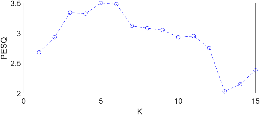
Figure 2: PESQ of different K

Discussion As we can see in Fig. 2, we show the variation curve of PESQ with different $K$. The highest PESQ = 3.48 when $K=5$. Thus, in Fig. 3, we show the Gaussian distributions corresponding to classes 1-5, and their parameters $\pi_{k},\mu_{k},\Sigma_{k}$ are shown. The sixth picture in Fig. 3 represents the original noisy signal and the estimated noisy signal. They overlap with each other, and the PESQ score is 3.48, which reflects that our proposed DiffGMM model can estimate complex noisy distributions.

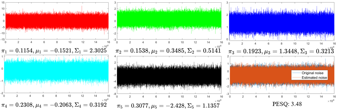
Figure 3: Five different Gaussian distributions are obtained through DiffGMM in the original audio. The figure shows the Gaussian distributions corresponding to classes 1-5, and their parameters $\pi_{k},\mu_{k},\Sigma_{k}$ are shown below. The sixth figure is the original noisy signal and the estimated noisy signal. The X-axis is the audio length, and the Y-axis is the audio range.

4 Conclusion

In this work, we develop a DiffGMM model, which is a denoising model based on the diffusion model and Gaussian mixture models. By employing the reverse process to estimate parameters for the Gaussian mixture model, our DiffGMM model can generalize the condition of Gaussian noise in the diffusion model to any noise distribution. Extensive experimental results demonstrate that the proposed DiffGMM model outperforms many state-of-the-art methods.

References

- [1] J. Li, P. Wang, and Y. Zhang, ``Deeplabv3+ vision transformer for visual bird sound denoising,'' IEEE Access, 2023.
- [2] S. Qi, Z. Huang, Y. Li, and S. Shi, ``Audio recording device identification based on deep learning,'' in 2016 IEEE International Conference on Signal and Image Processing (ICSIP), 2016, pp. 426–431.
- [3] N. Carlini and D. Wagner, ``Audio adversarial examples: Targeted attacks on speech-to-text,'' in 2018 IEEE Security and Privacy Workshops (SPW), 2018, pp. 1–7.
- [4] H. Schröter, T. Rosenkranz, A. N. Escalante-B, M. Aubreville, and A. Maier, ``Clcnet: Deep learning-based noise reduction for hearing aids using complex linear coding,'' in ICASSP 2020-2020 IEEE International Conference on Acoustics, Speech and Signal Processing (ICASSP). IEEE, 2020, pp. 6949–6953.
- [5] Y. Zhao, Z.-Q. Wang, and D. Wang, ``Two-stage deep learning for noisy-reverberant speech enhancement,'' IEEE/ACM transactions on audio, speech, and language processing, vol. 27, no. 1, pp. 53–62, 2018.
- [6] J. Li, P. Wang, J. Li, X. Wang, and Y. Zhang, ``Dpatd: Dual-phase audio transformer for denoising,'' in 2023 Third International Conference on Digital Data Processing (DDP). IEEE, 2023, pp. 36–41.
- [7] Y. Zhang and J. Li, ``Birdsoundsdenoising: Deep visual audio denoising for bird sounds,'' in Proceedings of the IEEE/CVF Winter Conference on Applications of Computer Vision, 2023, pp. 2248–2257.
- [8] S. Pascual, A. Bonafonte, and J. Serra, ``Segan: Speech enhancement generative adversarial network,'' arXiv preprint arXiv:1703.09452, 2017.
- [9] J. Li, D. Kang, W. Pei, X. Zhe, Y. Zhang, Z. He, and L. Bao, ``Audio2gestures: Generating diverse gestures from speech audio with conditional variational autoencoders,'' in Proceedings of the IEEE/CVF International Conference on Computer Vision, 2021, pp. 11 293–11 302.
- [10] M. Strauss and B. Edler, ``A flow-based neural network for time domain speech enhancement,'' in ICASSP 2021-2021 IEEE International Conference on Acoustics, Speech and Signal Processing (ICASSP). IEEE, 2021, pp. 5754–5758.
- [11] J. Ho, A. Jain, and P. Abbeel, ``Denoising diffusion probabilistic models,'' Advances in Neural Information Processing Systems, vol. 33, pp. 6840–6851, 2020.
- [12] N. G. Nair, W. G. C. Bandara, and V. M. Patel, ``Image generation with multimodal priors using denoising diffusion probabilistic models,'' arXiv preprint arXiv:2206.05039, 2022.
- [13] Y. Leng, Z. Chen, J. Guo, H. Liu, J. Chen, X. Tan, D. Mandic, L. He, X. Li, T. Qin et al., ``Binauralgrad: A two-stage conditional diffusion probabilistic model for binaural audio synthesis,'' Advances in Neural Information Processing Systems, vol. 35, pp. 23 689–23 700, 2022.
- [14] Y.-J. Lu, Y. Tsao, and S. Watanabe, ``A study on speech enhancement based on diffusion probabilistic model,'' in 2021 Asia-Pacific Signal and Information Processing Association Annual Summit and Conference (APSIPA ASC). IEEE, 2021, pp. 659–666.
- [15] R. Huang, M. W. Lam, J. Wang, D. Su, D. Yu, Y. Ren, and Z. Zhao, ``Fastdiff: A fast conditional diffusion model for high-quality speech synthesis,'' arXiv preprint arXiv:2204.09934, 2022.
- [16] C. Valentini-Botinhao et al., ``Noisy speech database for training speech enhancement algorithms and tts models,'' University of Edinburgh. School of Informatics. Centre for Speech Technology Research (CSTR), 2017.
- [17] Y. Zhang and J. Li, ``Complex Image Generation SwinTransformer Network for Audio Denoising,'' in Proc. INTERSPEECH 2023, 2023, pp. 186–190.
- [18] J. Li, J. Li, P. Wang, and Y. Zhang, ``Dcht: Deep complex hybrid transformer for speech enhancement,'' in 2023 Third International Conference on Digital Data Processing (DDP). IEEE, 2023, pp. 117–122.
- [19] Y.-J. Lu, Z.-Q. Wang, S. Watanabe, A. Richard, C. Yu, and Y. Tsao, ``Conditional diffusion probabilistic model for speech enhancement,'' in ICASSP 2022-2022 IEEE International Conference on Acoustics, Speech and Signal Processing (ICASSP). IEEE, 2022, pp. 7402–7406.
- [20] Y. Li, M. Sun, and X. Zhang, ``Perception-guided generative adversarial network for end-to-end speech enhancement,'' Applied Soft Computing, vol. 128, p. 109446, 2022.
- [21] H. Huang, R. Wu, J. Huang, J. Lin, and J. Yin, ``Dccrgan: Deep complex convolution recurrent generator adversarial network for speech enhancement,'' in 2022 International Symposium on Electrical, Electronics and Information Engineering (ISEEIE). IEEE, 2022, pp. 30–35.
- [22] D. Yin, C. Luo, Z. Xiong, and W. Zeng, ``Phasen: A phase-and-harmonics-aware speech enhancement network,'' in Proceedings of the AAAI Conference on Artificial Intelligence, vol. 34, 2020, pp. 9458–9465.
- [23] S. Fu, C. Yu, T. Hsieh, P. Plantinga, M. Ravanelli, X. Lu, and Y. M. Tsao, ``An improved version of metricgan for speech enhancement,'' arXiv preprint arXiv:2104.03538, 2021.
- [24] G. Yu, A. Li, C. Zheng, Y. Guo, Y. Wang, and H. Wang, ``Dual-branch attention-in-attention transformer for single-channel speech enhancement,'' in ICASSP 2022-2022 IEEE International Conference on Acoustics, Speech and Signal Processing (ICASSP). IEEE, 2022, pp. 7847–7851.
- [25] H. J. Park, B. H. Kang, W. Shin, J. S. Kim, and S. W. Han, ``Manner: Multi-view attention network for noise erasure,'' in ICASSP 2022-2022 IEEE International Conference on Acoustics, Speech and Signal Processing (ICASSP). IEEE, 2022, pp. 7842–7846.
- [26] K. Wang, B. He, and W.-P. Zhu, ``Tstnn: Two-stage transformer based neural network for speech enhancement in the time domain,'' in ICASSP 2021-2021 IEEE International Conference on Acoustics, Speech and Signal Processing (ICASSP). IEEE, 2021, pp. 7098–7102.
- [27] F. Dang, H. Chen, and P. Zhang, ``Dpt-fsnet: Dual-path transformer based full-band and sub-band fusion network for speech enhancement,'' in ICASSP 2022-2022 IEEE International Conference on Acoustics, Speech and Signal Processing (ICASSP). IEEE, 2022, pp. 6857–6861.
- [28] R. Cao, S. Abdulatif, and B. Yang, ``Cmgan: Conformer-based metric gan for speech enhancement,'' arXiv preprint arXiv:2203.15149, 2022.
- [29] X. Qin, Z. Zhang, C. Huang, M. Dehghan, O. R. Zaiane, and M. Jagersand, ``U2-net: Going deeper with nested u-structure for salient object detection,'' Pattern recognition, vol. 106, p. 107404, 2020.
- [30] H. Wang, S. Xie, L. Lin, Y. Iwamoto, X.-H. Han, Y.-W. Chen, and R. Tong, ``Mixed transformer u-net for medical image segmentation,'' in ICASSP 2022-2022 IEEE International Conference on Acoustics, Speech and Signal Processing (ICASSP). IEEE, 2022, pp. 2390–2394.
- [31] R. Strudel, R. Garcia, I. Laptev, and C. Schmid, ``Segmenter: Transformer for semantic segmentation,'' in Proceedings of the IEEE/CVF international conference on computer vision, 2021, pp. 7262–7272.
- [32] O. Ronneberger, P. Fischer, and T. Brox, ``U-net: Convolutional networks for biomedical image segmentation,'' in Medical Image Computing and Computer-Assisted Intervention–MICCAI 2015: 18th International Conference, Munich, Germany, October 5-9, 2015, Proceedings, Part III 18. Springer, 2015, pp. 234–241.
- [33] V. Badrinarayanan, A. Kendall, and R. Cipolla, ``Segnet: A deep convolutional encoder-decoder architecture for image segmentation,'' IEEE transactions on pattern analysis and machine intelligence, vol. 39, no. 12, pp. 2481–2495, 2017.
- [34] S. R. Park and J. Lee, ``A fully convolutional neural network for speech enhancement,'' arXiv preprint arXiv:1609.07132, 2016.
- [35] M. M. Kashyap, A. Tambwekar, K. Manohara, and S. Natarajan, ``Speech denoising without clean training data: A noise2noise approach,'' arXiv preprint arXiv:2104.03838, 2021.
- [36] E. Moliner and V. Välimäki, ``A two-stage u-net for high-fidelity denoising of historical recordings,'' in ICASSP 2022-2022 IEEE International Conference on Acoustics, Speech and Signal Processing (ICASSP). IEEE, 2022, pp. 841–845.