fast-resolve: Fast Bayesian Radio Interferometric Imaging

Abstract

Context. Interferometric imaging is algorithmically and computationally challenging as there is no unique inversion from the measurement data back to the sky maps, and the datasets can be very large. Many imaging methods already exist, but most of them focus either on the accuracy or the computational aspect.

Aims. This paper aims to reduce the computational complexity of the Bayesian imaging algorithm resolve, enabling the application of Bayesian imaging for larger datasets.

Methods. By combining computational shortcuts of the CLEAN algorithm with the Bayesian imaging algorithm resolve we developed an accurate and fast imaging algorithm which we name fast-resolve.

Results. We validate the accuracy of the presented fast-resolve algorithm by comparing it with results from resolve on VLA Cygnus A data. Furthermore, we demonstrate the computational advantages of fast-resolve on a large MeerKAT ESO 137-006 dataset which is computationally out of reach for resolve.

Conclusions. The presented algorithm is significantly faster than previous Bayesian imaging algorithms, broadening the applicability of Bayesian interferometric imaging. Specifically for the single channel VLA Cygnus A datasets fast-resolve is about $144$ times faster than resolve. For the MeerKAT dataset with multiple channels the computational speedup of fast-resolve is even larger.

1 Introduction

Interferometric imaging is a versatile technique in astronomy that allows us to achieve enormous sensitivity and resolution by combining multiple telescopes. The effective resolution is roughly equivalent to that of a single telescope with a diameter equal to the largest distance between individual stations of the interferometer, which can be thousands of kilometers. For the upcoming Square Kilometer Array (Labate et al. 2022; Swart et al. 2022), the total collecting area might eventually approach one square kilometer, resulting in superior sensitivity compared to any single-dish telescope. Overcoming the resolution and sensitivity limitations of single telescopes comes at the cost of making it more difficult to retrieve images from the observational data.

Mathematically, the recovery of the sky images from interferometric data can be formulated as an inverse problem. The forward relation that computes the corresponding measurement data from a given sky image is known as the radio interferometric measurement equation (Smirnov 2011). As discussed in detail in Sec. 2, the measured data points are essentially noisy and undersampled Fourier modes of the sky image. This makes direct inversion of the measurement equation to obtain the sky image impossible, turning radio interferometric imaging into an ill-posed inverse problem.

Solving the inverse problem of radio interferometric imaging requires sophisticated algorithms that impose additional constraints on the sky brightness and regularize possible solutions to it. Historically, CLEAN (Högbom 1974; Schwab & Cotton 1983) has been by far the most widely used imaging algorithm because it is computationally efficient, simple, and easy to use. Over the last decades, CLEAN-based imaging algorithms have been significantly improved, especially for diffuse emission imaging, spectral imaging, and wide-field imaging (Bhatnagar & Cornwell 2004; Cornwell et al. 2008; Rau & Cornwell 2011; Offringa et al. 2014; Offringa & Smirnov 2017). However, CLEAN-based algorithms have several drawbacks, such as limited image fidelity, suboptimal resolution of recovered images, and lack of uncertainty quantification (see eg. Arras et al. (2021a) for a detailed discussion). To improve these limitations, many other imaging algorithms have been developed.

A large class of new imaging algorithms builds on applying compressed sensing techniques to astronomical data (Wiaux et al. 2009). Several incarnations of such algorithms have shown significant improvements in terms of image fidelity and resolution over CLEAN based reconstructions. Recent examples are Dabbech et al. (2018); Abdulaziz et al. (2019); Dabbech et al. (2021) utilizing sparsity based regularizers in combination with convex optimization. Birdi et al. (2018, 2020) extended these approaches to full polarization imaging. In Repetti et al. (2019) and Liaudat et al. (2023), some form of uncertainty quantification was added. Dabbech et al. (2022); Thouvenin et al. (2023) parallelized the image regularizer to distribute it over multiple CPUs. Terris et al. (2023a); Dabbech et al. (2022) presented a regularizer building on a neural network image denoisers. Terris et al. (2023b) further explored neural network regularizers and studied the influence of the training dataset on the regularizer.

Bayesian imaging algorithms are another important class of imaging algorithms addressing the uncertainty quantification problem. Early Bayesian imaging approaches such as Cornwell & Evans (1985) built on the maximum entropy principle. Other Bayesian imaging techniques such as Sutton & Wandelt (2006); Sutter et al. (2014); Cai et al. (2018); Tiede (2022) rely on posterior sampling techniques. The Bayesian imaging framework resolve originally proposed by Junklewitz et al. (2016) builds on variational inference instead of sampling based techniques for posterior approximation, reducing the computational costs. resolve has already successfully been applied to VLA, EHT, VLBA, GRAVITY, and ALMA data, providing high-quality radio maps with superior resolution compared to CLEAN, as well as an uncertainty map. Recent examples are Arras et al. (2019) joining Bayesian imaging with calibration. In Arras et al. (2021a) resolve is compared with CLEAN, while in Roth et al. (2023), direction-dependent calibration is added and compared with sparsity based imaging results of Dabbech et al. (2021). In GRAVITY Collaboration et al. (2022) resolve is applied to the optical interferometer GRAVITY. In Arras et al. (2022) resolve is applied to EHT data.

The improvements in imaging algorithms mentioned above come at the cost of increased computational complexity. For Very Long Baseline Interferometer (VLBI) observations, data sizes are typically small and the higher computational cost of advanced imaging methods is unproblematic. However, for large arrays such as MeerKAT (Jonas & MeerKAT Team 2016), this limits the applicability of many of these algorithms. For this reason, only very few advanced imaging algorithms have so far been successfully applied to data sets the size of a typical MeerKAT observation. Dabbech et al. (2022) presents an application of an imaging algorithm using sparsity based and neural network regularizers to the MeerKAT ESO 137-006 observation. To handle the enormous computational complexity, Dabbech et al. (2022) massively parallelize their imaging algorithm and distribute it across a high performance computing system, requiring hundreds to thousands of CPU hours to converge. In Thouvenin et al. (2023), this approach of parallelizing the regularizer is extended to the spectral domain.

To the best of our knowledge, no Bayesian radio interferometric imaging algorithm has so far been applied to a similar sized dataset. The goal of the resolve framework has always been to enable Bayesian imaging for a wide range of radio telescopes, not just VLBI observations. However, for instruments such as MeerKAT, imaging with resolve becomes computationally prohibitively expensive. In this paper, we present the algorithm fast-resolve, which significantly reduces the computational complexity of classical resolve and enables Bayesian image reconstruction for large data sets. Greiner et al. (2016) previously already named an imaging method fastRESOLVE. The goal of the fastRESOLVE algorithm of Greiner et al. (2016) is the same as the new incarnation of fast-resolve presented in this paper. However, although the new and the old variants of fast-resolve share some ideas, there are significant differences. In Sec. 3.4, we will highlight the common concepts between the old the and the new fast-resolve. Note that the framework behind both fast-resolve and resolve has evolved significantly since the time of Greiner et al. (2016).

Machine learning-based imaging algorithms are a third relatively new class of imaging algorithms. Once the underlying machine learning models are trained, the computational cost for imaging is often lower than for other algorithms. Nevertheless, assessing image fidelity is challenging in such a framework given the lack of interpretability of machine learning models. Recent examples of such algorithms are Aghabiglou et al. (2024, 2023); Connor et al. (2022); Schmidt et al. (2022).

The remainder of the paper is organized as follows. In Sec. 2, we discuss the radio interferometric measurement equation and the imaging inverse problem in detail. In Sec. 3, we briefly review the existing resolve framework in its current form and outline the CLEAN algorithm. Building on some of the computational shortcuts of the CLEAN algorithm, we derive fast-resolve, and in Sec. 4, we show several applications of it. In particular, in Sec. 4.1 we compare imaging results of fast-resolve with the classical resolve framework on VLA (Perley et al. 2011) data to validate the fidelity of the resulting sky images, and in Sec. 4.2 we present a fast-resolve reconstruction of the ESO 137-006 MeerKAT observation to demonstrate the computational speedup.

2 The inverse problem

The radio interferometric measurement equation, derived, for example, in Smirnov (2011), relates the radio sky brightness to the datapoints, often called visibilities. More specifically, via the measurement equation, model visibilities $\tilde{V}$ can be computed for an assumed sky brightness $I$ and antenna sensitivity $G$. Under the assumption of scalar antenna gains $G$, the model visibility $\tilde{V}_{pqt}$ of antennas $p$ and $q$ at time $t$ is given as:

$$\tilde{V}_{pqt}=\int C(\boldsymbol{l},w_{pqt})I(\boldsymbol{l})G_{p}(t,\boldsymbol{l})G^{*}_{q}(t,\boldsymbol{l})e^{-2\pi i(\boldsymbol{k}_{pqt}\cdot\boldsymbol{l})}d\boldsymbol{l},$$ (1)

where

• $\boldsymbol{l}=(l,m)$ are the sky coordinates,

• $t$ is the time coordinate,

• $\boldsymbol{k}_{pqt}=(u_{pqt},v_{pqt})$ are the baseline uv-coordinates in units of the imaging wavelength,

• $C(\boldsymbol{l},w_{pqt})=\exp{\left(-2\pi iw_{pqt}\left(\sqrt{1-\boldsymbol{l}^{2}}-1\right)\right)}/\sqrt{1-\boldsymbol{l}^{2}}$ is the $w$- or non-coplanar baselines effect,

• $I(\boldsymbol{l})$ is the sky brightness,

• $G_{p}(t,\boldsymbol{l})$ is the gain of antenna $p$ depending on time and potentially also direction.

The model visibilities are therefore Fourier-like components of the sky brightness $I$ modulated by the antenna gains $G_{p}$ and $G_{q}$ as well as the $w$-effect $C$. The visibilities actually recorded in the measurement are related to the model visibilities according to

$$V_{pqt}=\tilde{V}_{pqt}+n=R(I)+n,$$ (2)

with $n$ representing some unknown noise in the measurement, and $R$ the mapping from sky brightness to visibilities defined in Eq. 1. With Eq. 1 and Eq. 2, it is straightforward to compute simulated visibilities for an assumed sky brightness $I$, antenna gain $G$, and noise statistics. Inverting this relation is not possible without additional assumptions, since first, the measured visibilities $V$ are corrupted by the measurement noise $n$, and second, Eq. 1 is generally not invertible since in practical applications not all Fourier components are measured.

The non-uniqueness of solutions to Eq. 2 means that additional regularisation needs to be imposed to discriminate between all possible sky images compatible with the data. This additional information is either an explicit prior or regularization term, or is implicitly encoded in the structure of the imaging algorithm.

3 Methods

In this section, we derive the fast-resolve algorithm (Sec. 3.3). Since fast-resolve builds on the already existing Bayesian imaging framework resolve, we start with a brief review of the classic resolve imaging method (Sec. 3.1). As some of the computational speedups of fast-resolve are inspired by the CLEAN imaging algorithm, we also outline the basic concepts behind CLEAN (Sec. 3.2).

3.1 resolve

The resolve imaging algorithm addresses the imaging inverse problem from a probabilistic perspective. Thus, instead of reconstructing a single estimate of the sky brightness, it infers the posterior probability distribution $P(I|V)$ of possible sky images given the measured visibilities. Bayes’ Theorem

$$P(I|V)=\frac{P(V|I)P(I)}{P(V)}$$ (3)

expresses the posterior probability $P(I|V)$ in terms of the likelihood $P(V|I)$, the prior $P(I)$, and the evidence $P(V)$. resolve provides models for the likelihood $P(V|I)$ and the prior $P(I)$. The posterior distribution can be inferred for a given prior and likelihood model building on the functionality of the Bayesian inference package NIFTy (Selig et al. 2013; Steininger et al. 2019; Edenhofer et al. 2024a). In the next three subsections we briefly outline the likelihood and prior of resolve as well as the variational inference algorithms of NIFTy.

3.1.1 resolve prior

The resolve framework provides predefined prior models for the two types of radio emission, point sources and extended diffuse emission. Both priors encode that the brightness must be positive, since there is no negative flux. Furthermore, both priors are very flexible and allow for brightness variations over several orders of magnitude.

For the point source prior, pixels are independently modeled with an inverse gamma prior for their intensity. The inverse gamma distribution is strictly positive and has a wide tail, allowing extremely bright sources. In the example in Sec. 4.1, such a prior is applied for the two bright point sources in the core of Cygnus A. While the brightness of point sources is reconstructed from the data, the locations currently need to be manually set. This limits the applicability of the current point source prior, as discussed in the application to MeerKAT ESO 137-006 data (Sec. 4.2).

Besides positivity and possible variations over several orders of magnitude, the diffuse emission prior also encodes correlations of the brightness of nearby pixels, which is essentially the defining property of diffuse emission. The correlation of nearby pixels in the diffuse emission prior is modeled by Gaussian processes. The result of the Gaussian process is exponentiated to ensure positivity. Detailed explanations of the resolve prior models can be found in Arras et al. (2021a). An important aspect of all the prior models in resolve is that they are fast and scalable to very large numbers of pixels. For example, in Arras et al. (2021a) a $4096\times 2048$ pixel Gaussian process-based diffuse emission prior is used to image Cygnus A at various frequencies.

3.1.2 resolve likelihood

The likelihood is evaluated in resolve using Eq. 1. More specifically, using Eq. 1, we can write the likelihood as $P(V|I)=P(V|R(I))=P(V|\tilde{V})$. The noise statistics in Eq. 2 then determines the likelihood. In resolve, Gaussian noise statistics are assumed. For numerical reasons, resolve works with the negative logarithm of the likelihood, named the likelihood Hamiltonian, instead of the likelihood itself. With the Gaussian noise assumption, the likelihood Hamiltonian is given by

$$H(V|I)=\frac{1}{2}\left(V-R(I)\right)^{\dagger}N^{-1}\left(V-R(I)\right)+\frac{1}{2}\ln|2\pi N|,$$ (4)

with $\dagger$ denoting complex conjugate transpose and $\frac{1}{2}\ln|2\pi N|$ coming form the normalization of the Gaussian, which can be ignored in many applications. Different possibilities are implemented for the covariance of the noise $N$. In the simplest case, the weights of the visibilities are used as the inverse noise covariance. Alternatively, the noise covariance can also be estimated during the image reconstruction.

The computationally important aspect of the likelihood in the classic resolve framework is that for every update step where the likelihood is evaluated, also $R(I)$ and thus Eq. 1 need to be computed. This can be computationally expensive, especially for datasets with many visibilities, as we will discuss in detail later.

3.1.3 resolve posterior inference

resolve is built on the probabilistic programming package NIFTy, which provides variational inference methods (Knollmüller & Enßlin 2019; Frank et al. 2021) to approximate the posterior distribution for a given prior and likelihood function. The advantage of variational inference techniques over sampling techniques such as MCMC or HMC is that they scale better with the number of parameters, which is the number of pixels in the imaging context. For example, the variational inference method of NIFTy has recently been used in a 3D reconstruction with 607 million voxels (Edenhofer et al. 2024b). While the variational inference algorithms scale very well with the number of parameters, they still need to evaluate the likelihood very often. This means variational inference is fast as long as the evaluation of the likelihood and prior is fast.

As discussed in Sec. 3.1.2, evaluating the likelihood in resolve boils down to evaluating the radio interferometric measurement equation (Eq. 1). To do so resolve relies on the parallelizable wgridder (Arras et al. 2021b) implemented in the ducc library. Nevertheless, evaluating the measurement equation becomes computationally intensive for data sets with many visibilities. For example, for the MeerKAT data set considered in Sec. 4.2, evaluating Eq. 1 on eight threads takes about $45$ seconds. This becomes prohibitive for algorithms which require many thousands of likelihood evaluations.

3.2 CLEAN

In this section, we briefly outline some of the concepts behind the CLEAN algorithm (Högbom 1974; Schwab & Cotton 1983), as the computational speedups of fast-resolve over classic resolve are partly inspired by CLEAN. We will refrain from delving into the details behind the numerous improvements that have been made to the CLEAN algorithm over the last decades (see Rau et al. (2009) for example) and focus only on the aspects which are relevant to speeding up resolve. We refer the reader to Arras et al. (2021a) for a detailed comparison between CLEAN and resolve.

CLEAN is an iterative optimization algorithm minimizing the weighted square residuals between the measured visibilities and the model visibilities computed from the sky brightness model. Expressed as a formula, the objective function minimized by CLEAN is identical to Eq.4, the likelihood Hamiltonian of resolve. Minimizing Eq. 4 with respect to the sky brightness $I$ is equivalent to solving

$$R^{\dagger}N^{-1}RI=R^{\dagger}N^{-1}V,$$ (5)

with $R^{\dagger}$ being the adjoint operation of $R$, thus mapping from visibilities to the sky brightness. Neglecting wide-field effects originating from non-coplanar baselines, the operation $R^{\dagger}N^{-1}R$ is, equivalent to a convolution with the effective point spread function of the interferometer $I^{\text{PSF}}$. $R^{\dagger}N^{-1}V$ is the back projection of the noise-weighted data into the sky domain, called dirty image $I^{\texttt{D}}$. This can be expressed with the formula

$$I^{\text{PSF}}*I\approx R^{\dagger}N^{-1}V=I^{\text{D}},$$ (6)

with $I^{\text{PSF}}$ being the PSF of the interferometer and $*$ denoting convolution. Thus, the dirty image $I^{\text{D}}=R^{\dagger}N^{-1}V$ is approximately the true sky brightness $I$ convolved with the PSF $I^{\text{PSF}}$ of the interferometer. Radio interferometric imaging is, therefore, nearly equivalent to deconvolving the dirty image.

As discussed in Sec. 2, no unique solution to imaging inverse problems exists. The absence of a unique solution manifests as $R^{\dagger}N^{-1}R$ and $I^{\text{PSF}}*$ not being invertible operations. While in resolve, additional regularization was provided via an explicit prior, regularization of the sky images in CLEAN is implicitly encoded into the structure of the algorithm. More specifically, CLEAN starts with an empty sky model as an initial estimate $I^{m}_{0}$ for the true sky brightness and iteratively adds components, in the simplest form point sources, to this estimate until a stopping criterion is met. This introduces the implicit prior that the sky is sparsely represented by a finite number of CLEAN components.

In the following, we briefly summarize the algorithmic structure of CLEAN as relevant for fast-resolve. The iterative procedure of adding components to the current model image $I^{m}$ is split into major and minor cycles. In the major cycles, a current residual image $I^{\text{RES}}=R^{\dagger}N^{-1}(V-RI^{m}_{i})$ is computed, with $I^{m}_{i}$ being the current model image. In the minor cycle, additional components are added to the model, and their PSFs are removed from the residual image. In the subsequent major cycle, the residual image is recomputed for the updated model image, and in the following new minor cycle, more components get added to the model. This scheme is iterated until a global stopping criterion is met.

From a computational perspective, the important aspect of the major/minor scheme is that $R$ and $R^{\dagger}$ only need to be evaluated in major cycles. In minor cycles, the PSF of the added CLEAN components is subtracted from the residual image, but for this, no evaluations of $R$ and $R^{\dagger}$ are needed since the PSF can be precomputed once. Most of the computations of the CLEAN algorithm are performed in image space, and only major cycles go back to the visibility space. In contrast, resolve needs to map from image to data space by applying $R$ for every likelihood evaluation.

3.3 fast-resolve

As outlined in the previous section, evaluating the radio interferometric instrument response (Eq. 1) contributes a substantial fraction to the overall runtime of a resolve image reconstruction. Therefore, reducing the number of necessary evaluations of Eq. 1 has the potential for significant speedups. The basic idea of fast-resolve is to perform most of the computations in image space, similar to CLEAN, and only evaluate the radio interferometric instrument response once in a while.

3.3.1 fast-resolve measurement equation

The radio interferometric measurement equation in the form of Eq. 2 leads to the likelihood Hamiltonian Eq. 4 of the classic resolve framework, which involves an evaluation of the interferometric instrument response $R$. To get a likelihood Hamiltonian that does not include evaluating $R$, one has to transform the measurement equation such that all involved quantities live in image space, not data space. To project all involved quantities to image space, we apply $R^{\dagger}N^{-1}$ from the left to Eq. 2, and get:

$$R^{\dagger}N^{-1}V =R^{\dagger}N^{-1}RI+R^{\dagger}N^{-1}n$$ (7)

$$I^{\text{D}} =R^{\prime}I+n^{\prime},$$ (8)

with $R^{\prime}=R^{\dagger}N^{-1}R$, and $n^{\prime}=R^{\dagger}N^{-1}n$. The quantities of the new measurement equation are $I^{\text{D}}$, $I$, and $n^{\prime}$ and are all defined in image space and not in data space. The statistics of the new noise $n^{\prime}$ remains Gaussian as $R^{\dagger}N^{-1}$ is a linear transformation. The corresponding likelihood Hamiltonian is given by:

$$H(I^{\text{D}}|I)=\frac{1}{2}(I^{\text{D}}-R^{\prime}I)^{\dagger}N^{\prime-1}(I^{\text{D}}-R^{\prime}I)+\frac{1}{2}\ln|2\pi N^{\prime}|.$$ (9)

The covariance of the transformed noise is given by

$$N^{\prime} =\left<n^{\prime}n^{\prime\dagger}\right>=R^{\dagger}N^{-1}\left<nn^{\dagger}\right>N^{-1}R=R^{\dagger}N^{-1}R.$$ (10)

This new noise covariance $N^{\prime}$ is not invertible as $R^{\dagger}N^{-1}R$ is not invertible, which is problematic as the likelihood Hamiltonian contains the inverse noise covariance $N^{\prime-1}$. To mitigate the problem of a singular noise covariance, we modify the measurement equation once more by adding uncorrelated Gaussian noise with a small amplitude. This leads to a noise covariance

$$N^{\prime}=R^{\dagger}N^{-1}R+\epsilon\mathbb{I},$$ (11)

with $\mathbb{I}$ being the unit matrix and $\epsilon$ a small number, which is the variance of the additional noise. With this artificially introduced additional noise, the full noise covariance $N^{\prime}$ is invertible, and the new likelihood Hamiltonian Eq. 9 becomes well defined.

3.3.2 fast-resolve response $R^{\prime}$

How large the speedup of using the new likelihood Hamiltonian Eq. 9 is compared to the old Hamiltonian Eq. 4 depends on how much faster the new Hamiltonian can be evaluated. The idea of fast-resolve is to approximate $R^{\prime}=R^{\dagger}N^{-1}R$ with a PSF convolution $R^{\prime}=R^{\dagger}N^{-1}R\approx I^{\text{PSF}}*$, as it is done in a similar way in the CLEAN algorithm. Approximating $R^{\prime}=R^{\dagger}N^{-1}R$ by a convolution with the PSF is only exact for coplanar arrays. Corrections for the inaccuracy of the approximation are applied in some major cycles in analogy to the CLEAN algorithm, as we describe in Sec. 3.3.4.

The convolution with the PSF $I^{\text{PSF}}*$ can be efficiently applied via an FFT convolution. For data sets with many visibilities, this FFT-based convolution with the PSF $I^{\text{PSF}}$ has the potential to be significantly faster than an evaluation of the interferometer response $R$ (Eq. 1). In Sec. 4, we will compare the computational speedup of the new likelihood for different data sets.

As the sky brightness $I$ and the PSF $I^{\text{PSF}}$ are non-periodic, some padding of the sky is needed for an FFT-based convolution. More specifically, to exactly evaluate $I^{\text{PSF}}*I$, the PSF with which we convolve needs to be twice as big as the field of view we want to image since some emission in the sky $I$ could be at the edge of the field we are imaging. The sky image needs to be padded with zeros to the same size as the PSF. As a formula, this can be noted as

$$R^{\prime}I =R^{\dagger}N^{-1}RI$$ (12)

$$\approx I^{\text{PSF}}*I$$ (13)

$$=P^{\dagger}\text{FFT}^{-1}\left[\text{FFT}[I^{\text{PSF}}]\cdot\text{FFT}[PI]\right],$$ (14)

with $P$ denoting the padding operation, and $P^{\dagger}$ for slicing out the region not padded. By neglecting PSF sidelobes and reducing its size, the necessary amount of zero padding can be reduced. This, however, reduces the accuracy of the approximation $R^{\prime}\approx I^{\text{PSF}}*$, which might make it necessary to perform more major cycles in the image reconstruction.

3.3.3 fast-resolve noise model

To evaluate the likelihood Hamiltonian of fast-resolve, we need to apply both $R^{\prime}=R^{\dagger}N^{-1}R$ and $N^{\prime-1}=(R^{\dagger}N^{-1}R+\epsilon\mathbb{I})^{-1}$. Similar to $R^{\prime}$, we need to approximate $N^{\prime-1}$ such that we can apply it without having to evaluate $R$ and $R^{\dagger}$ every time. The basic idea of the approximation of $N^{\prime-1}$ is the same as for $R^{\prime}$, thus replacing the exact operation with an FFT convolution. Expressed as a formula, we compute the application of $N^{\prime}$ to some input $x$ via

$$N^{\prime}(x)\approx\text{FFT}^{-1}\left[K\cdot\text{FFT}(x)\right],$$ (15)

with some appropriate Kernel $K$. The approximate noise covariance still needs to fulfill the mathematical properties of covariances, because for our Bayesian model, the likelihood is a probability and not just an arbitrary cost function. Therefore, the approximated noise covariance matrix needs to be Hermitian and positive definite. Specifically, for the convolution approximation, this implies that all entries of the convolution kernel $K$ must be real and strictly positive. To fulfill these constraints, we parameterize $K$ as

$$K_{\xi}=\exp\xi+\epsilon,$$ (16)

with $\epsilon$ as defined in Eq. 11 and $\xi$ being an implicitly defined real-valued vector. We set this vector $\xi$ such that it minimizes the square residual between the true and the approximate noise covariance when applied to a test image with a point source in the center. Thus $\xi$ is set to

$$\bar{\xi}=\text{argmin}_{\xi}\left(N^{\prime}(I_{\delta})-\text{FFT}^{-1}\left[(\exp\xi+\epsilon)\cdot\text{FFT}(I_{\delta})\right]\right)^{2}$$ (17)

with $I_{\delta}$ having a point source or delta peak in the center of the field of view and otherwise being zeros. In words, we approximate the noise covariance $N^{\prime}$ with an appropriate Kernel $K$ that yields a proper covariance by construction, is easy to invert, and minimizes the squared distance to the effect that $N^{\prime}$ has on a point source.

To evaluate the likelihood (Eq. 9) we need to apply $N^{\prime-1}$. We do this by convolving with the inverse kernel:

$$N^{\prime-1}(x)\approx\text{FFT}^{-1}\left[K_{\bar{\xi}}^{-1}\cdot\text{FFT}(x)\right].$$ (18)

This involves a second approximation, as we here implicitly assume periodic boundary conditions. As long as the main lobe of the PSF is much smaller than the field of view, this assumption does not create large errors.

3.3.4 fast-resolve inference scheme

The previous sections derived the approximate likelihood for fast-resolve inspired by the CLEAN algorithm. In the same spirit, we adapt the major/minor cycle scheme of CLEAN to utilize it with Bayesian inference for a probabilistic sky brightness reconstruction. In the minor cycles, we optimize the current estimate of the posterior distribution $P(I|V)$ for the sky brightness $I$ using the above approximations for a fast likelihood evaluation. In the major cycles, we apply, similar to CLEAN, the exact response operations to correct for the approximation error.

The algorithm starts by initializing the dirty image $I^{\text{D}}=R^{\dagger}N^{-1}V$ from the visibilities $V$ using the exact response function $R$. The dirty image is the input data $d_{0}=I^{\text{D}}$ for the first minor cycle. The first minor cycle computes an initial estimate of the posterior distribution $P_{0}$ of the sky brightness using the measurement equation

$$d_{0}=I^{\text{PSF}}*I+n^{\prime},$$ (19)

with the approximations discussed in Sec. 3.3.2 and Sec. 3.3.3. We will discuss the exact algorithm used to estimate the posterior distribution in Sec. 3.3.5. From this initial estimate of the posterior distribution $P_{0}$, we compute the posterior mean of the sky brightness $I_{0}=\left<I\right>_{P_{0}}$. The posterior mean $I_{0}$ is the output of the first minor cycle and the input to the first major cycle. The first major cycle computes the residual $d_{1}$ between the dirty image $I^{\text{D}}$ and the posterior mean of the first minor cycle passed through the response $R^{\dagger}N^{-1}R$ of the fast resolve measurement equation:

$$d_{1}=I^{\text{D}}-R^{\dagger}N^{-1}RI_{0}.$$ (20)

In contrast to the minor cycle, $R^{\dagger}N^{-1}R$ is here computed exactly and not approximated with $I^{\text{PSF}}*$. The residual $d_{1}$ is the output of the major cycle and the input to the second minor cycle. In the second minor cycle, the posterior $P_{1}$ of $I$ for the measurement equation

$$d_{1}=I^{\text{PSF}}*(I-I_{0})+n^{\prime},$$ (21)

is approximated. This approximation can be done efficiently by starting with the posterior estimate of the previous minor cycle and refining this estimate. The output of the second minor cycle is the updated posterior mean $I_{1}=\left<I\right>_{P_{1}}$ which is the input to the next major cycle computing the new residual to the dirty image using the exact response:

$$d_{2}=I^{\text{D}}-R^{\dagger}N^{-1}RI_{1}.$$ (22)

The new residual data $d_{2}$ is the input to the next minor cycle. This scheme is iterated until converged, thus until no significant structures are left in the residual $d_{n}$ and the posterior estimates $I_{n}$ are not changing anymore. In algorithm 1 the full inference scheme is summarized as a pseudocode algorithm.

Algorithm 1 fast-resolve inference scheme

# compute dirty image

$I^{\text{D}}\leftarrow R^{\dagger}N^{-1}V$

# initialize input with dirty image

$d_{0}\leftarrow I^{\text{D}}$

# reconstruct $n$ major cycles

for i in $0\ldots n-1$ do

     # minor cycle

     estimate $P_{i}(I)$ from $d_{i}=I^{\text{PSF}}*I+n^{\prime}$

     # compute posterior mean

     $I_{i}\leftarrow\left<I\right>_{P_{i}}$

     

     # major cycle updating input data

     $d_{i+1}\leftarrow I^{\text{D}}-R^{\dagger}N^{-1}RI_{i}$

# final result: $P_{n-1}(I)$

The overall structure of the fast-resolve major/minor scheme is very similar to the major/minor scheme of CLEAN. The main difference is that fast-resolve updates in the minor cycles a probability distribution for possible sky images instead of a simple model image, as is the case for CLEAN. The algorithm for inferring the posterior distribution is outlined in the following subsection 3.3.5.

3.3.5 fast-resolve minor cycles

In the minor cycles, we optimize the approximation of the posterior distribution $P(I|V)$ using the scalable variational inference algorithms (Knollmüller & Enßlin 2019; Frank et al. 2021) of the NIFTy package already employed in the classic resolve algorithm. These variational inference algorithms account for correlations between parameters of the model. While the method Metric Gaussian Variational Inference (MGVI) of Knollmüller & Enßlin (2019) relies on a Gaussian approximation of the posterior distribution, the algorithm geometric Variational Inference (geoVI) of Frank et al. (2021) can also capture non-Gaussian posterior distributions. Although fast-resolve relies for the minor cycles on the same inference algorithms as resolve, updating the posterior distribution is much faster in fast-resolve since the approximate likelihood described above is used instead of evaluating the exact measurement equation.

Furthermore, the NIFTy package has also undergone a major rewrite, switching from a NumPy based (Harris et al. 2020) implementation to a JAX (Bradbury et al. 2018) based backend, allowing for GPU-accelerated computing. While resolve was so far building on the old NumPy-based NIFTy, fast-resolve makes use of the JAX accelerated NIFTy version, also named NIFTy.re (Edenhofer et al. 2024a). Especially the FFT convolutions in fast-resolve have the potential for significant GPU acceleration. In Sec. 4, we compare the runtime of resolve and fast-resolve using the CPU and the GPU backend.

In the future, we also plan to port the classic resolve framework to JAX. Porting resolve is more involved than porting fast-resolve because it requires binding a high performance implementation of the radio interferometric measurement operator to JAX. As a preparatory work, we have developed the JAXbind package (Roth et al. 2024) which allows to bind custom functions to JAX. However, since the wgridder from ducc is used to evaluate the radio interferometric measurement equation, the JAX version of resolve will also be limited to run on the CPU.

3.4 Previous fastRESOLVE of Greiner et al. (2016)

The algorithm named fastRESOLVE introduced by Greiner et al. (2016) was an earlier attempt to speed up resolve. Similar to the fast-resolve of this work, Greiner et al. (2016) used approximations of the likelihood avoiding applications of $R$ in every step. More specifically, Greiner et al. (2016) derived a maximum a posteriori estimator of the sky brightness using the gridded weights of the visibilities as a noise covariance. Since fastRESOLVE had some limitations, such as it could not account for the w-term and could not provide uncertainty estimates, this approach was not followed up in subsequent developments of resolve in Arras et al. (2019, 2021a), or Roth et al. (2023).

4 Applications

For verification, we demonstrate the proposed fast-resolve method on different data sets. First, we reconstruct the Cygnus A VLA observation at four different frequency bands, and second, we image ESO 137-006 using a MeerKAT observation. The Cygnus A data is suitable to validate the accuracy as the fast-resolve images can be compared to previous results from Arras et al. (2021a) and Roth et al. (2023) obtained on the same dataset. The Cygnus A reconstruction has a relatively small field of view, and wide field effects should be negligible. The MeerKAT observation is significantly larger than the VLA observation, and imaging with resolve is computationally out of reach, allowing to demonstrate the computational advantages of fast-resolve over resolve. Furthermore, the field of view of the ESO 137-006 observations is also significantly larger such that the major cycles of fast-resolve correcting for wide field effects become more important.

4.1 Application to VLA Cygnus A data

4.1.1 Data and algorithm setup

For imaging Cygnus A, we use the exact same data already imaged in Arras et al. (2021a) with resolve and CLEAN. The data contains single frequency channels at $2052\,\text{MHz}$ (S-band), $4811\,\text{MHz}$ (C-band), $8427\,\text{MHz}$ (X-band), and $13360\,\text{MHz}$ (Ku-band). Also, in Roth et al. (2023), an uncalibrated version of the S-band data was jointly calibrated and imaged with resolve. In all observing bands, all four VLA configurations were used. Computationally relevant details of the observations, such as the number of visibilities and the grid size of the reconstructed images, are listed in Tab. 1. For details on the calibration of the data, we refer to Sebokolodi et al. (2020).

Table 1: VLA Cygnus A observations. All observations are single channel and used all four VLA configurations. For all frequencies the same field of view (Fov) is imaged.

Freq [MHz]	$N_{rows}$	image size	Fov [deg]
2052	1281930	$512\times 1024$	$0.025\times 0.05$
4811	1281934	$1024\times 2048$	$0.025\times 0.05$
8427	2523954	$2048\times 4096$	$0.025\times 0.05$
13360	2544102	$2048\times 4096$	$0.025\times 0.05$

As a prior model, we use the combination of the diffuse emission prior and the point source prior described in Sec. 3.1.1. This prior model is identical to the prior model already used in the existing resolve framework. Specifically, in Arras et al. (2021a) and Roth et al. (2023), this prior model was already used for Cygnus A reconstructions. For completeness, we summarize the main aspects of the prior model here. We refer to Arras et al. (2021a) for details on the prior model. We model the diffuse emission with an exponentiated Gaussian Process spanning the entire field of view. For the two point sources in the nucleus of Cygnus A, we insert two separate point source models at the locations of these sources. For the brightness of these sources we use an inverse gamma prior. The exact hyper-parameters for the Gaussian process and the inverse gamma prior are listed in appendix A. The number of pixels used to model the diffuse emission is listed in Tab. 1 for the different frequencies.

In Arras et al. (2021a), the MGVI algorithm was used for inferring the posterior of the sky brightness map. For direct comparability between the results of this work and the previous resolve maps, we also use the MGVI in the minor cycles (Sec. 3.3.5) for the posterior approximation. For the imaging of the S-band data in Roth et al. (2023), the geoVI algorithm was used. However, we do not expect significant differences in the resulting sky maps.

To summarize, Arras et al. (2021a) and Roth et al. (2023) used the same prior model setup as we use for imaging Cygnus A with fast-resolve. Furthermore, the posterior inference algorithm is expected to produce similar results for a given likelihood. Therefore, the previous resolve results of Arras et al. (2021a) and Roth et al. (2023) are ideally suited to validate the fast-resovle likelihood approximation in a direct comparison on a dataset with negligible wide field effects. Furthermore, we compare with the multi-scale CLEAN reconstruction of the S-band data from Arras et al. (2021a). For a more detailed comparison with CLEAN, we refer to Arras et al. (2021a), where resolve was extensively compared to single and multi-scale CLEAN for all frequency bands.

4.1.2 Comparison with previous resolve results

In the following, we compare the fast-resolve reconstructions with previous results to validate the accuracy of fast-resolve. Fig. 1 displays the resolve reconstructions of Arras et al. (2021a) and Roth et al. (2023) as well as the S-band data multi-scale CLEAN reconstruction in comparison with the fast-resolve reconstructions of this work. The overall quality of the fast-resolve maps is on par with the resolve results. The multi-scale CLEAN reconstruction has a lower resolution in bright regions of the lobes than the resolve based reconstructions. All bright emission features are consistently reconstructed by all algorithms in all frequency bands. The fast-resolve and CLEAN maps have a higher dynamic range than the results of Arras et al. (2021a). Nevertheless, this is not due to a conceptional problem of the resolve algorithm, but rather the reconstructions of Arras et al. (2021a) were not fully converged due to the very high computational cost of resolve. resolve reconstructs the brightest emission of the field before modeling fainter features. Thus, faint features are missing in the radio map when a reconstruction is stopped before convergence. For fast-resolve, where the overall runtime of the algorithm is much shorter, it is easier to ensure that the reconstruction is fully converged. In Sec. 4.1.3 the convergence of resolve and fast-resolve is analyzed in detail. The resolve reconstruction of Roth et al. (2023) has a similar dynamic range compared to the fast-resolve reconstructions.

In the comparison between CLEAN and resolve in Arras et al. (2021a), resolve produced significantly higher resolved maps than CLEAN in regions with high surface brightness. A zoom into such a region, the eastern hotspot of Cygnus A, is depicted in Fig. 2. In this region, the results are consistent, and fast-resolve achieves the same resolution as the resolve based reconstructions. Furthermore, fast-resolve also shows minimal imaging artifacts around the hotspot, as does resolve. The multi-scale CLEAN map from Arras et al. (2021a) is added again for comparison. As already discussed in Arras et al. (2021a), the CLEAN reconstruction has a significantly lower resolution than the resolve reconstruction. These super-resolution capabilities where validated by comparing the morphological features of the resolve reconstructions with higher frequency observations under the assumption of spectral smoothness.

Fig. 3 zooms on the nucleus and jet of Cygnus A. In the zooms on the nucleus the pixels modeling the two point sources are clearly visible. The fast-resolve S-band reconstruction and the resolve reconstruction of Roth et al. (2023) show consistent results depicting the nucleus and jet. In the S-band reconstruction of Arras et al. (2021a), the jet is also visible, although due to the smaller dynamic range of the map, it is less pronounced. In the higher frequency bands, the shape of the core of Cygnus A is consistent between the reconstructions of resolve and fast-resolve. As the old resolve reconstructions are not fully converged, their dynamic range is lower, and the fainter emission of the jet is barely visible at higher frequencies. At the highest frequencies $13360\,\text{MHz}$, the jet is also barely visible in the fast-resolve reconstruction. The CLEAN image of the jet is consistent with the fast-resolve reconstruction and the resolve reconstruction from Roth et al. (2023).

resolve as well as fast-resolve provide posterior samples of the sky brightness distribution. From these samples, not only the posterior mean but also other summary statistics can be computed. As an example, we show in Fig. 4 the pixel-wise relative uncertainty of the S-band data reconstruction of fast-resolve in comparison with the corresponding uncertainty map of Arras et al. (2021a). The estimated uncertainty of resolve tends to be slightly higher than the uncertainty estimate of fast-resolve. This difference might come from the fact that the resolve reconstruction of Arras et al. (2021a) was not fully converged since the uncertainty estimate of resolve usually becomes smaller when the algorithm converges. Nevertheless, we cannot exclude that this is related to the approximations of fast-resolve.

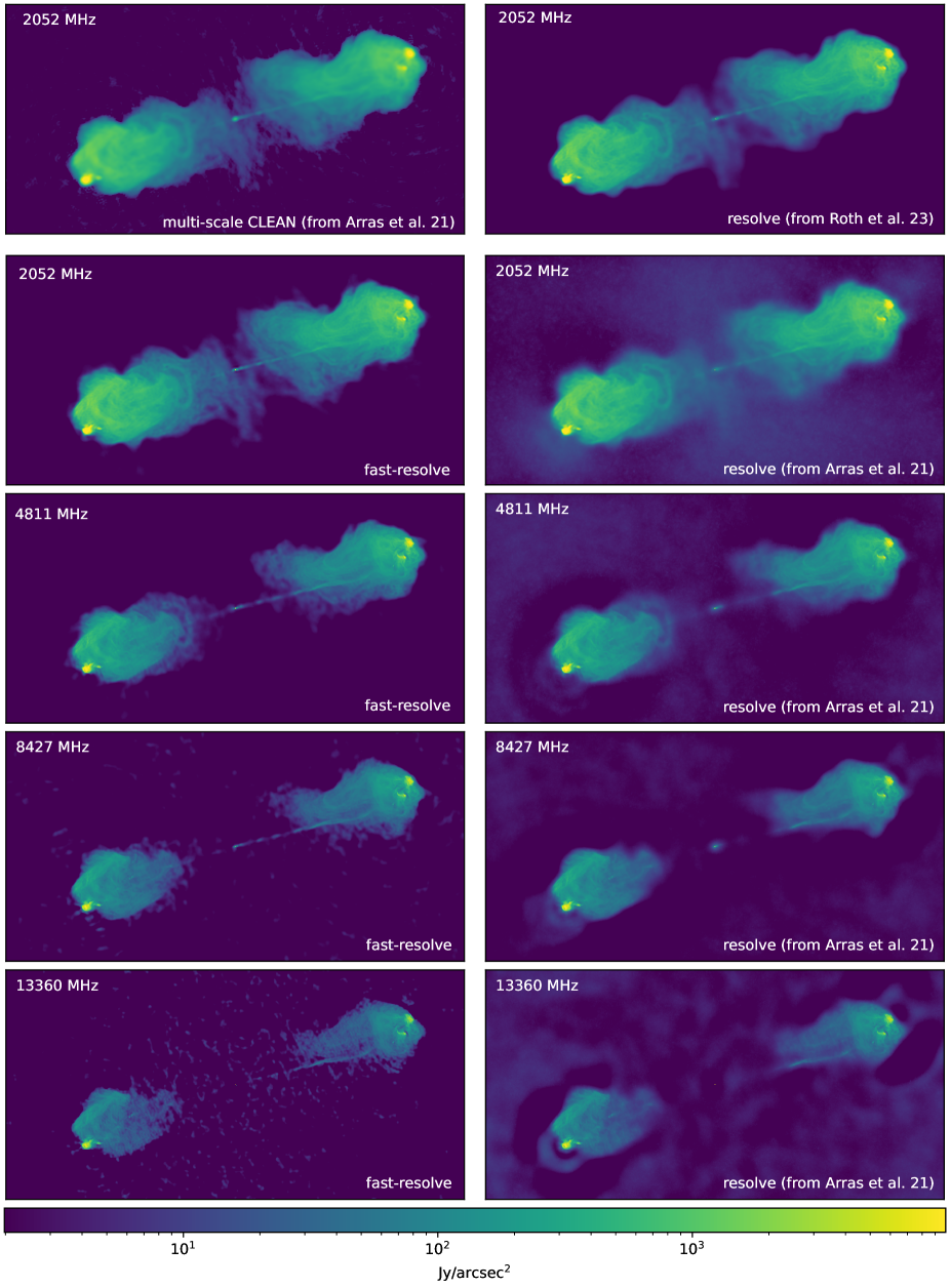
Figure 1: Comparison of fast-resolve Cygnus A reconstructions with resolve and CLEAN reconstructions. The top left panel shows the multi-scale CLEAN map of the S-band data form Arras et al. (2021a). The left column below the CLEAN map shows fast-resolve reconstructions at four different frequencies indicated in the top left corner of each panel. The right column shows resolve reconstructions of Roth et al. (2023) and Arras et al. (2021a) using the same data. The dynamic range of the fast-resolve reconstructions is higher than in some of the previous resolve reconstructions. This is because the old resolve reconstructions were not fully converged due to their high computational cost.

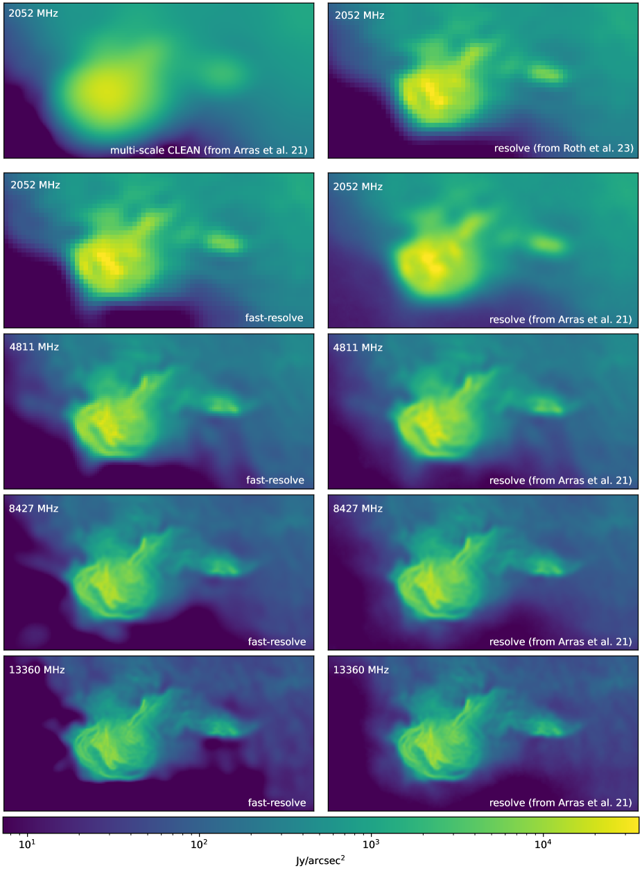
Figure 2: Zoom on the eastern hot spot of the Cygnus A reconstructions from Fig. 1. The resolution of the fast-resolve maps in the left column is on par with the resolve maps in the right column. The resolution of the CLEAN map is significantly lower than the in the other maps.

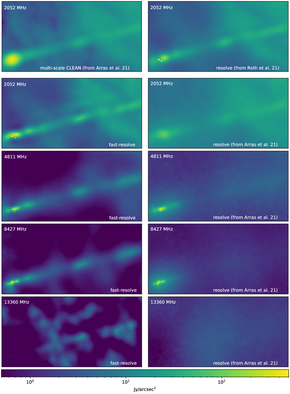
Figure 3: Zoom on the nucleus and jet of the Cygnus A reconstructions form Fig. 1. In all resolve and fast-resolve reconstructions, the two point sources in the nucleus are modeled with two pixels that are uncorrelated with the brightness of the neighboring pixels. Since the resolve of Arras et al. (2021a) are not fully converged due to their high computational cost, their dynamic range is lower, and the jet of Cygnus A is not visible. The multi-scale CLEAN map from Arras et al. (2021a) is consistent with the fast-resolve result and the resolve reconstruction from Roth et al. (2023). At the highest frequency the jet is hardly visible also with fast-resolve, with background artifacts having a similar brightness.

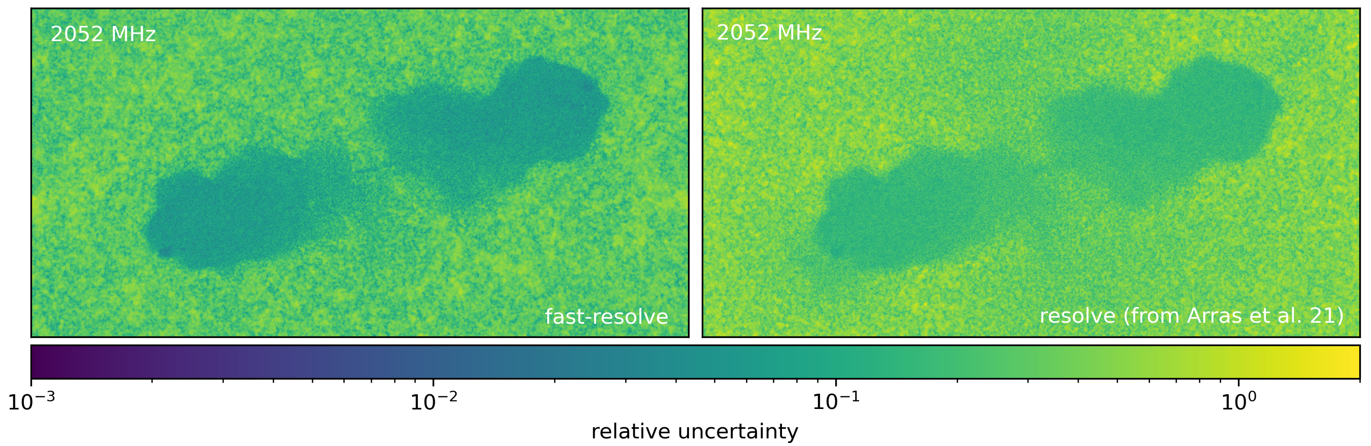
Figure 4: Pixel-wise relative uncertainty map of fast-resolve S-band reconstruction compared to the resolve uncertainty map of Arras et al. (2021a). The relative uncertainty is lower for both reconstructions in regions of high surface brightness. In the hotspot, the relative uncertainty is around $10^{-3}$ to $10^{-2}$ and increases towards the lower surface brightness regions. Outside of Cygnus A, the relative uncertainty fluctuates around $1$, indicating that the reconstructed intensity is statistically consistent with zero surface brightness. The estimated uncertainty of resolve tends to be slightly higher than the uncertainty estimate of fast-resolve. This might be due to the resolve reconstruction of Arras et al. (2021a) not being fully converged.

4.1.3 Computational time of fast-resolve

In the previous subsection, we compared the results of fast-resolve with resolve, confirming that fast-resolve can deliver the same high quality radio maps as resolve. In this subsection, we want to analyze the computational speed of fast-resolve and compare it to the existing resolve framework. To have a direct comparison between the runtimes, we imaged the S-band data with exactly the same hyperparameters for the prior model with fast-resolve and resolve and saved snapshots of the reconstructions at several points during the optimization. While resolve can only be executed on a CPU, fast-resolve can also run on a GPU.

Fig. 5 depicts the direct comparison between resolve and fast-resolve, with both algorithms being executed on the same CPU. Specifically, the algorithms were run on an Intel Xeon W-1270P CPU with $3.80\,\text{GHz}$ clock speed and $8$ cores. For the resolve reconstruction, the MGVI algorithm inferring the posterior distribution was parallelized with $4$ MPI tasks, each using $2$ cores for evaluating the radio interferometric measurement equation (Eq. 2), thus utilizing $8$ cores in total. The fast-resolve reconstruction ran on the single python process without manual threading, relying on JAX to parallelize the computations over the cores. Snapshots of the reconstructions after $10$, $60$, $300$, $600$, and $1440\,\text{min}$ are displayed. After $10\,\text{min}$, the hotspot and parts of the lobes are visible in the reconstructions of both algorithms. Nevertheless, the core and the jet are missing, and both reconstructions have significant background artifacts. After $60\,\text{min}$ runtime, fainter parts of the lobes become visible, and the fast-resolve map shows significantly more details in the lower surface brightness regions. After $300\,\text{min}$ the fast-resolve map also depicts the very low surface brightness regions with high resolution, while in the resolve map, the outflow is still partially missing, and the lower surface brightness regions of the lobes are reconstructed with low resolution. After $600\,\text{min}$ the fast-resolve map has only slightly changed compared to the $300\,\text{min}$ snapshot. At this point, we assume the fast-resolve algorithm to be fully converged. The resolve reconstruction is also after $600\,\text{min}$ not yet fully converged. The final snapshot of the resolve reconstruction is after $1440\,\text{min}$. At this stage also the resolve reconstruction is nearly converged. Only in the very low surface brightness regions of the lobes, the resolution is still lower than in the fast-resolve reconstruction.

While Fig. 5 analyzes the convergence of fast-resolve on the CPU, fast-resolve is mainly designed for GPUs. The performance of fast-resolve on the S-band data using GPUs is shown in Fig. 6. Specifically, Fig. 6 displays snapshots of the fast-resolve reconstruction after $1$, $5$, $10$, $22$, and $46\,\text{min}$ using an NVIDIA A100 high-performance computing GPU compared with a reconstruction on a consumer-level GPU, an NVIDIA GeForce RTX 3090. When comparing the results, one should consider that the A100 GPU is on the order of 10 times more expensive than the RTX 3090. On both GPUs, we executed the exact same fast-resolve reconstruction we ran on a CPU in Fig. 5. Similar to the CPU run, the high surface brightness regions are reconstructed first before the method picks up the low surface brightness flux. On both GPUs, the algorithm is much faster than on the CPU. While on the CPU, the reconstruction was finished after $600\,\text{min}$, the same number of major and minor cycles were finished on the RTX 3090 GPU in $46\,\text{min}$ and on the A100 GPU in $22\,\text{min}$. Thus, the fast-resolve reconstruction was 13 times faster on the RTX 3090 GPU and 27 times faster on the A100 GPU than the CPU reconstruction. In comparison, the resolve reconstruction on the CPU was not fully converged even after $1416\,\text{min}$.

To quantify the convergence rate of the reconstructions, we computed the mean square residual between the logarithmic brightness of the final fast-resolve iteration on the NVIDIA A100 GPU and earlier iterations of resolve and fast-resolve reconstructions. We reran the fast-resolve reconstructions with different random seeds to be independent of the random seed used for the NVIDIA A100 reconstruction with respect to which the residuals are computed. Fig. 7 shows the mean square residuals for resolve and the three fast-resolve reconstructions as a function of wall time. The fast-resolve reconstructions converge within the displayed time, and their curves of the mean square residual flatten. The reconstruction’s final mean square residuals are not exactly the same since the final maps are not numerically identical because of the different hardware, JAX, and CUDA versions. The resolve reconstruction does not converge in the displayed time interval and the residual error keeps falling until the end after $1416\,\text{min}$ ($1$ day). Of course, using the residual of the logarithmic brightness is an arbitrary metric for quantifying convergence speed. Nevertheless, it can roughly quantify the speedups of fast-resolve. After $1416\,\text{min}$, the mean square residual of the resolve reconstruction is around $10^{-3}$. In comparison, the fast-resolve reconstructions reach the same mean squared residual after around $10\,\text{min}$, $20\,\text{min}$, and $200\,\text{min}$ for runs on the NVIDIA A100 GPU, the NVIDIA RTX 3090 GPU and the Intel Xeon CPU, respectively. Thus, the indicative speedup of fast-resolve over resolve on the Cygnus A S-band data is a factor of $144$ for the A100 GPU, a factor of $72$ for the RTX 3090 GPU and a factor of $7.2$ for the CPU run. The timings reported above do not include the time needed to precompute the convolution kernels for the response and noise of fast-resolve. Nevertheless, these are small compared to the time needed for imaging. For the S-band data, for example, the computation of the kernels takes only $0.6\,\text{min}$, which is much shorter than the imaging runtime, even on the GPU.

As indicated in Tab. 1, the Cygnus A data has only a single frequency channel. For datasets with more baselines and frequency channels, such as the MeerKAT datasets considered in the next section (see Tab. 2), the algorithmic advantage of fast-resolve of not having to compute the radio response in each evaluation of the likelihood is much larger. Thus, for such datasets, the speedup of fast-resolve will be significantly larger than for the Cygnus A single channel imaging. Indeed for the MeerKAT dataset of the next section (Sec. 4.2) imaging with resolve is computationally out of scope, while with fast-resolve images can still be reconstructed with moderate computational costs.

The same comparison as in Fig. 6 but for the C-band data is displayed in Fig. 8. As indicated in Tab. 1, the grid size we used for the C-band sky map is a factor of two larger along both spatial axes. Thus, in total, we have four times more pixels, increasing the computational cost of the algorithm. On the A100 GPU, the fast-resolve reconstruction was finished after $56\,\text{min}$, while on the RTX 3090 GPU, the reconstruction took $165\,\text{min}$. We believe that the larger difference between the two GPUs for the C-band data compared to the S-band data might be because, for the smaller grid size of the S-band reconstruction, the A100 GPUs were not fully utilized.

For completeness, we also display snapshots of the X and Ku-band reconstructions in Fig. 9. These reconstructions were only carried out on the A100 GPU. After $132\,\text{min}$ both reconstructions were finished.

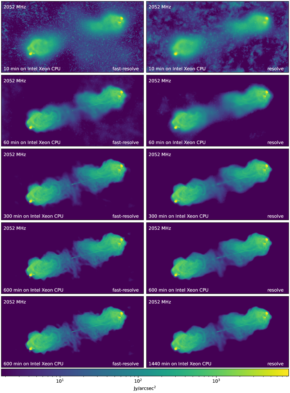
Figure 5: fast-resolve and resolve reconstructions of the $2052\,\text{MHz}$ Cygnus A data at different stages of the reconstruction. The left column shows fast-resolve the right column resolve. The rows display snapshots of the reconstruction after different amounts of wall time indicated in the lower left of each panel. The fast-resolve reconstruction was performed on two cores of an Intel Xeon CPU. The resolve reconstruction used eight cores of the same CPU. The fast-resolve reconstructions in the last two rows are at identical time snapshots, since the fast-resolve reconstruction is considered to be converged after $600\,\text{min}$. The resolve reconstruction is not fully converged even after $1416\,\text{min}$.

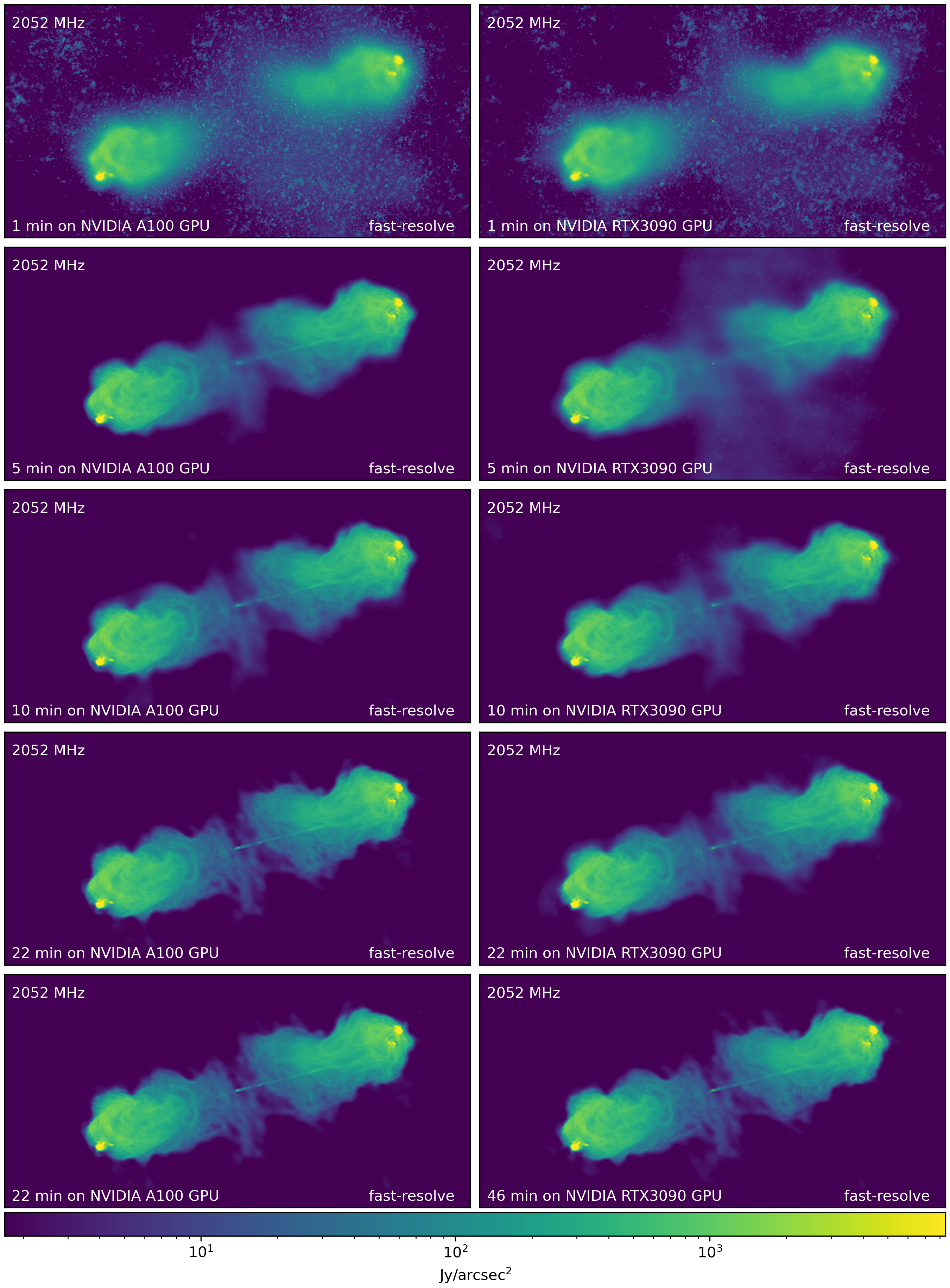
Figure 6: fast-resolve reconstructions of the $2052\,\text{MHz}$ Cygnus A data. The left column displays snapshots of a fast-resolve reconstruction on an NVIDIA A100 GPU. The right column shows snapshots of a fast-resolve reconstruction on an NVIDIA RTX 390 GPU. Both reconstructions ran the same number of major and minor iterations. Since the reconstruction on the A100 GPU was finished after $22\,\text{min}$, the bottom left panel is identical to the row above. On the A100 GPU fast-resolve is approximately twice as fast as on a RTX 390 GPU, and 25 times faster than on the CPU displayed in Fig. 5.

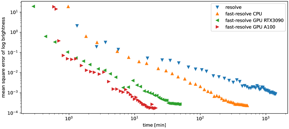
Figure 7: Mean square residual of the log brightness of resolve and fast-resolve reconstruction as a function of time for the S-band data. The residual is computed to the final iteration of fast-resolve on the NVIDIA A100 GPU depicted in Fig. 6, which we believe to be converged. The fast-resolve reconstructions are recomputed with a different random seed. The mean square residual of the fast-resolve reconstructions falls until their curves flatten when they converge. Due to the different hardware, JAX, and CUDA versions, the final results are numerically not exactly identical. The resolve reconstruction (blue curve) does not fully converge in the displayed time range.

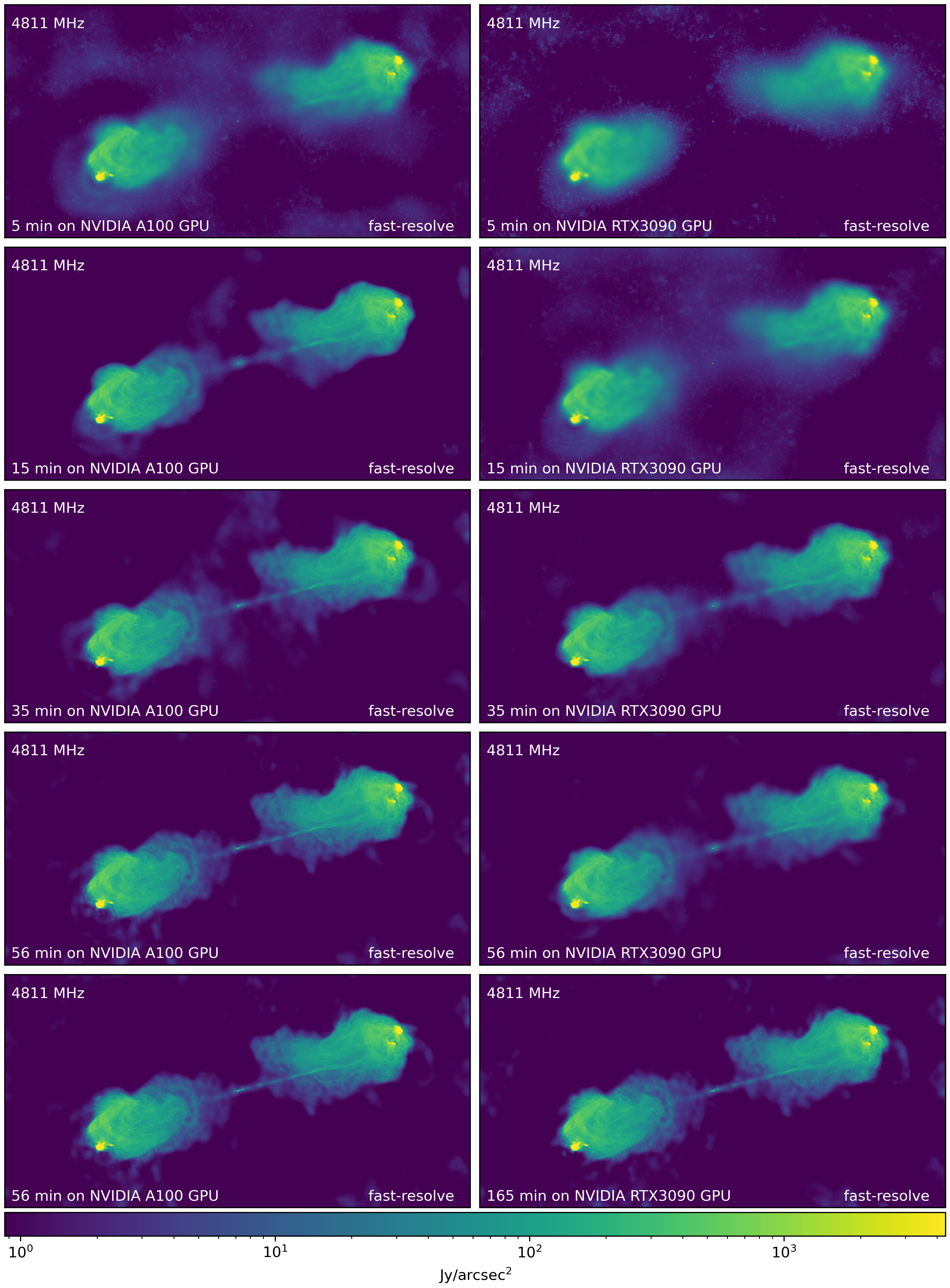
Figure 8: Same as Fig. 6 but for the $4811\,\text{MHz}$ data. On an NVIDIA A100 GPU fast-resolve is $2-3$ times faster than on an NVIDIA RTX 3090 GPU. The same number of major and minor iterations are performed on both GPUs. Since the reconstruction on the A100 GPU is finished after $56\,\text{min}$, the bottom left panel is identical to the row above.

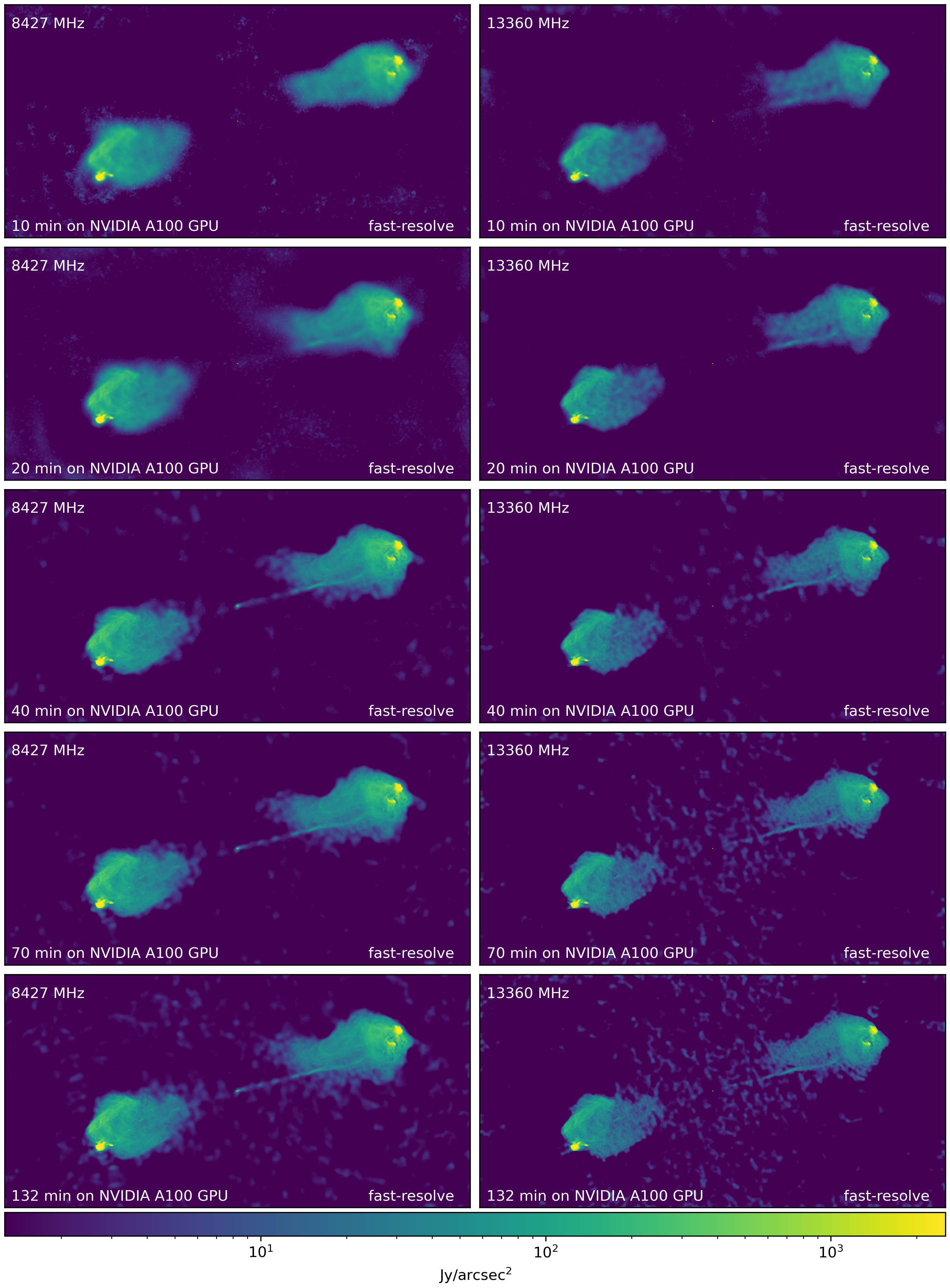
Figure 9: Snapshots of the fast-resolve Cygnus A reconstruction of the $8427\,\text{MHz}$ and $13360\,\text{MHz}$ data on a NIFTy A100 GPU. The wall time after which the snapshot was taken is indicated in the bottom left of each panel.

4.2 Application to MeerKAT data

In this section, we present an application of fast-resolve to an L-band ($856-1712\,\text{MHz}$) MeerKAT (Jonas & MeerKAT Team 2016) observation of the radio galaxy ESO 137-006. Originally, this observation was presented in Ramatsoku et al. (2020). The observation utilized all 64 MeerKAT antennas and the 4k mode of the SKARAB correlator. The total on target observation time is $14\,\text{h}$ in full polarization with $4096$ channels. For the VLA Cygnus A observations above, only a single frequency channel was used for each band. Here, we use two sub-bands with each about $200$ channels (after averaging) and a bandwidth of approximately $200\,\text{MHz}$. Consequently the MeerKAT datasets are more than $400$ times larger than the VLA datasets of the previous section, making an evaluation of the radio interferometer response (Eq. 1) significantly more expensive. A resolve reconstruction, where the exact response needs to be computed for each evaluation of the likelihood (Eq. 3.1.2), is computationally unfeasible for such a dataset.

Ramatsoku et al. (2020) detected hitherto unknown collimated synchrotron threads linking the lobes of the radio galaxy ESO 137-006 in this observation. Since then, this data set has also been used by Dabbech et al. (2022) for demonstrating a sparsity-based imaging algorithm. Dabbech et al. (2022) also published the results as FITS files, allowing us to use them as a reference for validating the fast-resolve algorithm for a MeerKAT-sized reconstruction.

Technical details relating to the initial flagging and transfer calibration of the ESO 137-006 data using the CARACAL pipeline (Józsa et al. 2020) are given in Ramatsoku et al. (2020). As in Ramatsoku et al. (2020), the data is averaged from 4096 to 1024 frequency channels and split into two sub-bands spanning $961-1145\,\text{MHz}$ and $1295-1503\,\text{MHz}$ that are relative free from radio frequency intereference, known as the LO and HI bands respectively. These subbands are then phase self-calibrated using WSClean multi-scale CLEAN (Offringa & Smirnov 2017) for imaging and CubiCal (Kenyon et al. 2018) for calibration. We then image the data independently in the LO and HI band with fast-resolve. Computational relevant details of the calibrated data in the two bands are listed in Tab. 2.

Table 2: MeerKAT ESO 137-006 observations. For both frequency bands the same field of view (Fov) is imaged.

Freq [MHz]	$N_{rows}$	$N_{chan}$	image size	Fov [deg]
961-1145	4598424	220	$3600\times 3600$	$2\times 2$
1295-1503	4598424	248	$3600\times 3600$	$2\times 2$

4.2.1 fast-resolve prior model

As for the Cygnus A observation, we built our prior model around the exponentiated Gaussian process model described in Sec. 4.1.1 and in detail in Arras et al. (2021a). Nevertheless, for the MeerKAT observation, there is, besides the main source, ESO 137-006, also a second galaxy, ESO 137-007, in the field of view. Due to the nature of the generative prior models in resolve, the full prior model can easily be composed of multiple components. We model each of these sources with a separate exponentiated Gaussian process to decouple the prior models. Furthermore, due to the high sensitivity of MeerKAT, many compact background sources are detected. For the Cygnus A reconstruction, we placed two point source models at the locations of the two point sources in the core of Cygnus A. However, for the MeerKAT observation, the number of background sources is far too large to manually place point source models at their locations. Therefore, we use a third Gaussian process model to represent all the background sources outside of the models for ESO 137-006 and ESO 137-007. A sketch of the layout of the three models is shown in Fig. 10. The exact parameters for all Gaussian process models are listed in appendix B.

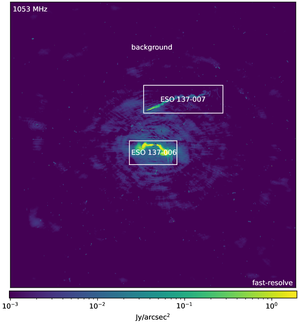
Figure 10: Reconstruction of the ESO 137-006 MeerKAT observation in the LO subband ($961-1145\,\text{MHz}$) with fast-resolve. The radio galaxies ESO 137-006 and ESO 137-007, as well as the background sources, are modeled with independent Gaussian processes. White boxes indicate the spatial extent of each Gaussian process. Zooms on the reconstructions of ESO 137-006 and ESO 137-007 for both subbands are shown in Fig. 11, 12, 13, and 14.

4.2.2 Imaging of Dabbech et al. (2022)

In Dabbech et al. (2022), ESO 137-006 is imaged with WSClean (Offringa et al. 2014; Offringa & Smirnov 2017) and two convex optimization algorithms in the same bands $961-1145\,\text{MHz}$ and $1295-1503\,\text{MHz}$ using the same data as we do. The two convex optimization algorithms of Dabbech et al. (2022) utilize two different regularizers. One regularizer is named uSARA, promoting sparsity in a wavelet basis. The other regularizer, AIRI, originally presented in Terris et al. (2023a), is based on a neural network denoiser. The resulting images for both regularizers are compared with results from WSClean, showing significant improvements in the image quality. The exact computational costs of all three imaging algorithms are reported in Dabbech et al. (2022). Imaging with the sparsity promoting regularizer, uSARA needed about $1500$ to $3000$ CPU hours per band to converge. With the neural network-based denoiser AIRI, around $900$ to $1600$ CPU hours plus around $5$ GPU hours where needed.

4.2.3 Imaging results

Fig. 10 depicts the results of the fast-resolve reconstruction for the LO band data. Zooms on the two radio galaxies are shown in Fig. 11 and Fig. 12 for the LO band and in Fig. 13 and Fig. 14 for the HI band. Thereby, Fig. 11 and Fig. 13 display the ESO 137-006 radio galaxy while Fig. 12 and 14 show the radio galaxy ESO 137-007 north of it. These figures also include the convex optimization reconstruction results of Dabbech et al. (2022) for comparison and validation. The imaging results of fast-resolve and Dabbech et al. (2022) are consistent. The fast-resolve maps have higher background artifacts than the convex optimization maps. In Ramatsoku et al. (2020), collimated synchrotron threads between the two lobes of the galaxy ESO 137-006 were detected. Besides these already known threads, the fast-resolve map shows additional threads north of the core of the galaxy. These additional threads are probably artifacts in the image. With a lower intensity, similar features are also found in the maps of Dabbech et al. (2022) and are mostly considered artifacts.

We believe these features are imaging artifacts and originate from suboptimal calibration. Due to the very flexible prior model, both fast-resolve and resolve are very sensitive the data. In the case of suboptimal calibration, this leads to imaging artifacts. At present, self-calibration with fast-resolve is not yet possible. For the future, the integration of a self-calibration routine into fast-resolve is planned, which could potentially mitigate such artifacts.

Additionally, a dedicated prior model for compact sources could improve the fast-resolve reconstructions. At present, point sources can either be modeled by manually placing inverse gamma distributed pixels at their locations (see Sec. 3.1.1) or by including them in the Gaussian process model. For the VLA Cygnus A reconstruction, the point sources in the nucleus were modeled by manually placing inverse gamma distributed pixels at their locations. Thereby, imaging artifacts around the two-point source could be avoided, despite them being very bright. Due to the high number of background sources, this is impractical for the ESO 137-006 reconstruction. Compact sources are therefore also modelled using an exponentiated Gaussian process prior. A dedicated prior model that is also applicable to observations with a very high number of background sources could improve their reconstruction.

4.2.4 Computational costs

Despite the high number of visibilities and frequency channels, the computational costs of fast-resolve are still moderate since fast-resolve only needs to evaluate the full radio interferometric measurement equation (Eq. 1) in the major cycles. The fast-resolve reconstructions of both frequency bands were done on an NVIDIA A100 GPU. Before the actual fast-resolve imaging, the convolution kernels for the response and the noise were constructed on a CPU. For both frequency bands, less than two hours were needed on a single core of an Intel Xeon CPU to compute the convolution kernel. For imaging, 24 hours using an NVIDIA A100 GPU and eight cores of an Intel Xeon CPU were needed. Since most of the fast-resovle operators, except for the major update steps, are done on the GPU, the CPU was mostly idle during imaging. In comparison, the computational costs of the Dabbech et al. (2022) reconstructions are significantly higher as they range between $900$ and $3000$ CPU hours per band and algorithm. Dabbech et al. (2022) for comparison also presented a WSClean reconstruction. For the WSClean reconstruction Dabbech et al. (2022) report a total computational cost of $132$ and $236$ CPU hours for the two imaging bands. Although CPU and GPU hours are not directly comparable, this underlines the computational performance and applicability of fast-resolve to imaging setups with massive datasets.

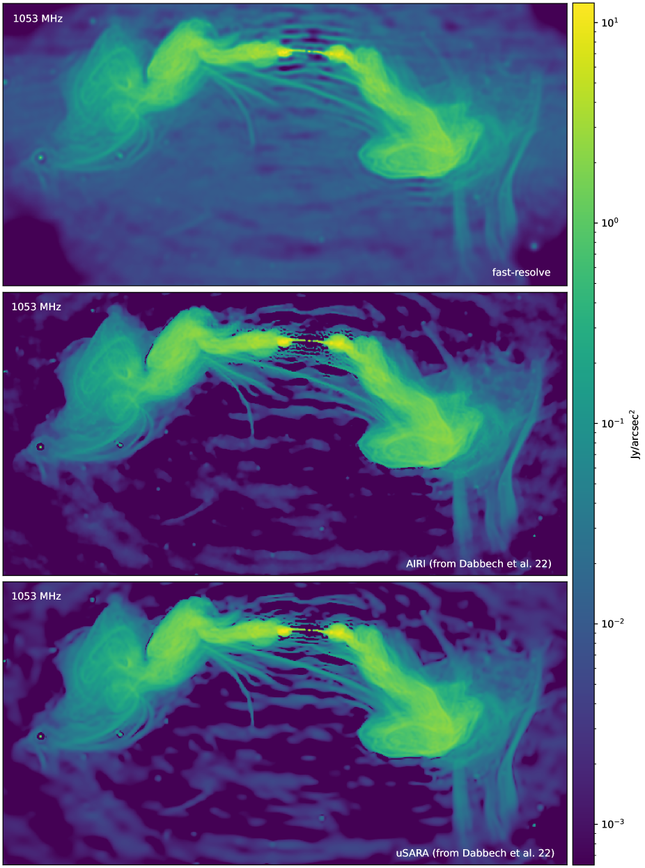
Figure 11: Radio Galaxy ESO 137-006 in the phase center of the observation. The top panel shows the fast-resolve reconstruction. For comparison the lower two panels display the reconstructions form Dabbech et al. (2022) with the AIRI and uSARA regularizers. All reconstructions, but especially fast-resovle, are affected by the suboptimal calibration.

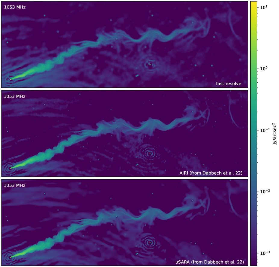
Figure 12: Radio Galaxy ESO 137-007 north of the phase center of the observation. The top panel shows the fast-resolve reconstruction. For comparison the lower two panels display the reconstructions form Dabbech et al. (2022) with the AIRI and uSARA regularizers. All reconstructions, but especially fast-resovle, are affected by the suboptimal calibration.

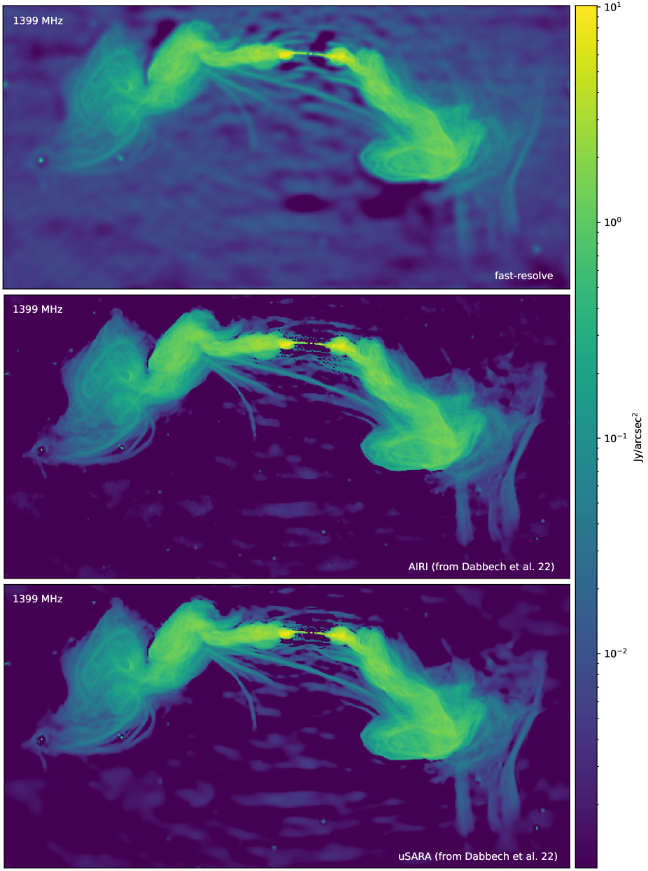
Figure 13: Like Fig. 11 but at $1399\,\text{MHz}$.

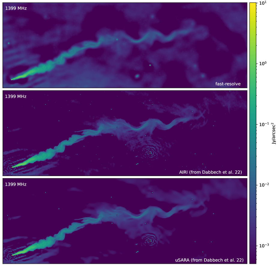
Figure 14: Like Fig. 12 but at $1399\,\text{MHz}$.

5 Conclusion

This paper introduces the fast Bayesian imaging algorithm fast-resolve. fast-resolve combines the accuracy of the Bayesian imaging framework resovle with computational shortcuts of the CLEAN algorithm. This significantly broadens the applicability of Bayesian radio interferometric imaging. fast-resolve transforms the likelihood of the Bayesian radio interferometric imaging problem into a likelihood of a deconvolution problem, which is much faster to evaluate. Using the major/minor cycle scheme of CLEAN, fast-resolve corrects for inaccuracies of the transformed likelihood and accounts for the w-effect. The accuracy of fast-resolve is validated on Cygnus A VLA data by comparing with previous resolve and multi-scale CLEAN reconstructions. The comparison shows that fast-resolve achieves the same resolution as resolve. Likewise, the imaging artifacts are comparable and on a very low level.

Furthermore, the computational speed of fast-resolve is analyzed and compared to resolve, showing significant speedups for the VLA Cygnus A data. As fast-resolve is implemented in JAX, it can also be executed on a GPU, accelerating the reconstruction compared to the CPU by more than an order of magnitude. For the single channel Cygnus A VLA dataset, fast-resolve is at least $140$ times faster than resolve when executed on a GPU. For datasets with more frequency channels, the computational advantages of fast-resolve can be even larger.

Additionally, we present a Bayesian image reconstruction of the radio galaxies ESO 137-006 and ESO 137-007 from MeerKAT data with fast-resolve and compare the results for validation with Dabbech et al. (2022). The MeerKAT dataset is significantly larger than the VLA datasets, but the computational costs of fast-resolve remain moderate due to the major/minor cycle scheme. A reconstruction of these sources with the classic resolve algorithm using the same amount of data would be computationally out of scope. To the best of our knowledge, no other Bayesian radio interferometric imaging algorithm has been successfully applied to a dataset of similar size before.

6 Data Availability

The raw data of the Cygnus A observation is publicly available in the NRAO Data Archive under project ID 14B-336. The raw data for the ESO137-006 observation is publicly available via the SARAO archive (project ID SCI-20190418-SM-01). The fast-resolve reconstruction results are archived on zenodo. The implementation of the fast-resolve algorithm will be integrated into the resolve algorithm.

Appendix A Prior parameters for Cygnus A imaging

In Tab. 3 we list the hyper parameters of the Gaussian process model for the diffuse emission in the Cygnus A reconstructions. The exact definition of these parameters is explained in detail in Arras et al. (2021a).

Table 3: Prior parameters for Cygnus A reconstructions

Cygnus A, band:	S	C	X	Ku
zero mode offset	18	21	20	20
zero mode mean	1	1	1	1
zero mode stddev	0.1	0.1	0.1	0.1
fluctuations mean	5	5	5	5
fluctuations stddev	1	1	1	1
loglogavgslope mean	-2	-2	-2.2	-2.2
loglogavgslope stddev	0.2	0.2	0.2	0.2
flexibility mean	1.2	1.2	1.2	1.2
flexibility stddev	0.4	0.4	0.4	0.4
asperity mean	0.2	0.2	0.2	0.2
asperity stddev	0.2	0.2	0.2	0.2

Appendix B Prior parameters for ESO 137 imaging

In Tab. 4 we list the hyper parameters of the Gaussian process model for the diffuse emission in the ESO 137 reconstructions. The exact definition of these parameters is explained in detail in Arras et al. (2021a).

Table 4: Prior parameters for ESO 137 reconstructions. For the two frequency bands, the LO ( $961-1145\,\text{MHz}$) and the HI ( $1295-1503\,\text{MHz}$) band we used the same hyper parameters.

ESO 137	006	007	background
zero mode offset	13	13	13
zero mode mean	1	1	1
zero mode stddev	0.1	0.1	0.1
fluctuations mean	3	4	4
fluctuations stddev	1	1	1
loglogavgslope mean	-2.4	-2.4	-2.0
loglogavgslope stddev	0.1	0.1	0.1
flexibility mean	0.1	0.1	1.2
flexibility stddev	0.01	0.1	0.4
asperity mean	0.01	0.01	0.2
asperity stddev	0.001	0.001	0.2