Optimal Control of Agent-Based Dynamics under Deep Galerkin Feedback Laws

Abstract

Ever since the concepts of dynamic programming were introduced, one of the most difficult challenges has been to adequately address high-dimensional control problems. With growing dimensionality, the utilisation of Deep Neural Networks promises to circumvent the issue of an otherwise exponentially increasing complexity. The paper specifically investigates the sampling issues the Deep Galerkin Method is subjected to. It proposes a drift relaxation-based sampling approach to alleviate the symptoms of high-variance policy approximations. This is validated on mean-field control problems; namely, the variations of the opinion dynamics presented by the Sznajd and the Hegselmann-Krause model. The resulting policies induce a significant cost reduction over manually optimised control functions and show improvements on the Linear-Quadratic Regulator problem over the Deep FBSDE approach.

I INTRODUCTION

Deep Learning has been shown to be an effective tool in finding the solution of high-dimensional PDEs [sirignano, exarchos, weinan-e, weinan-e2, raissi, al-aradi]. With the application of the Deep Galerkin Method to stochastic optimal control problems, the appropriate sampling of batches on domain and boundary becomes a major challenge. This is especially the case when considering the dynamics of interacting agents. We show how the sampling technique may prohibit the Deep Galerkin loss from converging to zero and propose a simple algorithm to alleviate this issue. The approach is evaluated on the controlled consensus dynamics represented by the Szanjd model [sznajd] and the Hegselmann-Krause Model [hegselmann].

In contrast to open-loop control, feedback control laws do not depend on a specific initial condition and are significantly more robust to perturbations. Optimal feedback controllers can be composed from the solution of the respective Hamilton-Jacobi-Bellman equation. The solution of this partial differential equation, however, becomes intractable in higher-dimensional problems. In the case of unconstrained linear control systems with quadratic cost, the Hamilton-Jacobi-Bellman equation reduces to an Algebraic Riccati equation. This has been extensively studied in [kalman] early on in 1960. The first significant approaches on nonlinear control systems with a scalar control variable were made in [albrekht]. The authors’ method involved a power series expansion of the involved terms around the origin. They inserted these back into the Hamilton-Jacobi-Bellman equation and collected expressions of similar order. He obtained a sequence of algebraic equations part of which conveniently reduce to the Riccati equation. Each of these expressions can be solved. The solution is a local solution in a neighbourhood around the origin. More recent efforts focused on semi-Lagrangian schemes [bokanowski] [falcone]. These work similarly to Finite Difference Methods. However, they also employ an interpolation scheme for the region surrounding grid points. Like other grid-based approaches, these methods do not scale well to higher dimensions. The authors of [alla] alleviate this issue by coupling grid-based discretisations of low-dimensional Hamilton-Jacobi-Bellman equations. They base this method on the concept of proper orthogonal decomposition; a technique that is well known from computational fluid dynamics. However, the quality of these schemes has been shown to deteriorate in highly nonlinear or advection affected settings such as presented in [kalise2]. In [kang], they compute approximate solutions to Hamilton-Jacobi-Bellman equations by combining the method of characteristics with sparse space discretisations. This works similarly to the semi-Lagrangian schemes. First, they solve on a very coarse grid using the characteristic equations, then, polynomial interpolations are used to obtain approximations at arbitrary points. This approach is causality-free, i.e. it does not directly depend on the density of the grid and is, therefore, more suitable for high-dimensional problems. Alternative implementations based on tensor decomposition have also been proven successful in tackling dimensionality issues [stefansson]. [dolgov] extended such framework to fully nonlinear, first-order, stationary Hamilton-Jacobi-Bellman PDEs. Nevertheless, the curse of dimensionality remains a challenge. There are several causality-free deep learning algorithms that are applicable to high-dimensional stochastic optimal control. The idea of using data-driven value function approximations is not new. An early record of this is [munos] in which a neural network was utilised to model the solution to the Hamilton-Jacobi-Bellman equation associated with the control of a car in a one-dimensional landscape. FBSDE-based methods such as in [raissi], [exarchos], or [weinan-e2] solve the associated system of Forward-Backward SDEs. This is realised by integration over a time-discretised domain of path realisations. Another idea relies on the minimisation of the residuals of the Hamilton-Jacobi-Bellman PDE [al-aradi] [sirignano] [nguyen]. This concept is termed the Deep Galerkin Method and forms the foundation of this paper. Opinion dynamics models such as in [sznajd] and [hegselmann] are governed by interacting diffusion processes. Their models are the basis to the realisation of the endeavour to enforce coherent behaviours in large populations. The control of these is manifested as a mean-field control problem. [kalise] approximates the optimal policy via a hierarchy of suboptimal controls. Instead, the proposal is, here, to employ a Deep Galerkin approach.

The paper is structured as follows. In Section II, we introduce the relevant background later sections build on. This includes information regarding the general concepts in Stochastic Optimal Control, the Hamilton-Jacobi-Bellman equation, and the Deep Galerkin Method. Subsection II-D goes more into detail about the type of problems considered, while Section III exemplifies the sampling issues that appear with the Deep Galerkin Method when considering the optimal control of interacting, stochastic agents. The proposed methodology is evaluated in the last section. The code repository is available at https://github.com/FreditorK/Optimal-Control-of-Agent-Based-Dynamics.

II BACKGROUND

II-A Stochastic Optimal Control

We study a finite horizon problem over the interval $[t,T]$ subjected to nonlinear stochastic dynamics as represented by an Itô process. We denote by $(\Omega,\mathcal{F},\{\mathcal{F}_{t}\}_{t\geq 0},\mathbb{P})$ a filtered probability space and by $\mathbb{A}\subseteq L^{2}([t,T]\times\Omega;\mathbb{P})$ the space of admissible control functions. We consider the optimisation problem

$$\inf_{\upsilon\in\mathbb{A}}\; \mathbb{E}^{\mathbb{P}}\Big{[}\int_{t}^{T}F(s,X_{s},\upsilon(s,X_{s}))ds+G(X_{T})\;\Big{|}\;X_{t}=x\Big{]}$$

s.t. $$dX_{s}=\mu(s,X_{s},\upsilon(s,X_{s}))ds+\sigma(s,X_{s},\upsilon(s,X_{s}))dW_{s}$$

$$X_{0}\sim\nu,$$ (2)

where $X_{s}\in\Omega\subseteq\mathbb{R}^{n}$ is an $\{\mathcal{F}_{s}\}_{s\geq 0}$-adapted Itô process, $\mu:\mathbb{R}\times\mathbb{R}^{n}\times\mathbb{R}\mapsto\mathbb{R}^{n}$, $\sigma:\mathbb{R}\times\mathbb{R}^{n}\times\mathbb{R}\mapsto\mathbb{R}^{n\times m}$, and $W_{s}$ is an $m$-dimensional Brownian motion. The initial distribution of the process $\{X_{s}\}_{s\geq 0}$ is denoted by $\nu$. Additionally, the objective is specified by a cost function $F:\mathbb{R}\times\mathbb{R}^{n}\times\mathbb{R}\mapsto\mathbb{R}^{+}$ and a terminal cost $G:\mathbb{R}^{n}\mapsto\mathbb{R}^{+}$. These are assumed to be non-negative bounded from below and continuous.

II-B The Hamilton-Jacobi-Bellman Equation

We denote by $J:\mathbb{R}\times\mathbb{R}^{n}\mapsto\mathbb{R}$ the optimal value function such that

$$J(t,x)=\inf_{\upsilon\in\mathbb{A}}\; \mathbb{E}^{\mathbb{P}}\Big{[}\int_{t}^{T}F(s,X_{s},\upsilon(s,X_{s}))ds+G(X_{T})\;\Big{|}\;X_{t}=x\Big{]}$$

By Bellman’s Optimality Principle, the value function $J$ satisfies the Hamilton-Jacobi-Bellman equation

$$\begin{cases}0=\partial_{t}J(t,x)+\underset{u\in\mathbb{R}}{\min}\{\mathcal{L}^{u}J(t,x)+F(t,x,u)\}\\ J(T,x)=G(x)\end{cases},$$

$$\text{where }\mathcal{L}^{u}:=\mu(s,X_{s},u)\cdot\nabla+\frac{1}{2}\sigma(s,X_{s},u)\sigma(s,X_{s},u)^{T}:D^{2}$$

with $u$ being substituted in as the optimal control value closed-loop control process within $\mathbb{R}$. $D^{2}$ represents the Hessian operator here. Under the assumption that the Hamiltonian $H(t,x,u)=\mathcal{L}^{u}J(t,x)+F(t,x,u)$ is differentiable and the space of admissible control functions is unconstrained, the optimal control process can often times be recovered by solving $\frac{d}{du}H(t,x,u)=0$. The examples in this paper make use of this property.

II-C The Deep Galerkin Method

Let $u$ represent the optimal control signal at time $t$. The Deep Galerkin Method [sirignano] aims to minimise the residuals of the differential terms of the $\theta$-parametrised neural network $J_{\theta}$ to the solution of the Hamilton-Jacobi-Bellman equation $J$. Given an equation

$$\begin{cases}0=\partial_{t}J(t,x)+\mathcal{L}^{u}J(t,x)+F(t,x,u)\\ J(T,x)=G(x)\end{cases}.$$

we minimise the error $\mathcal{E}(J_{\theta};[t,T]\times\Omega)$ composed of

$$\mathcal{E}(J_{\theta};[t,T]\times\Omega)= w_{1}||(\partial_{s}+\mathcal{L}^{u})(J_{\theta}-J)||_{L^{2}([t,T]\times\Omega;\nu_{1})}$$

$$+w_{2}||J_{\theta}(T,\cdot)-G||_{L^{2}(\Omega;\nu_{2})}$$

$$= w_{1}||(\partial_{s}+\mathcal{L}^{u})J_{\theta}+F||_{L^{2}([t,T]\times\Omega;\nu_{1})}$$

$$+w_{2}||J_{\theta}(T,\cdot)-G||_{L^{2}(\Omega;\nu_{2})}.$$ (3)

The respective norms are weighted with the scalars $w_{1},w_{2}\in\mathbb{R}$ and are approximated by taking the mean of the squared residual over $\nu_{1}$- and $\nu_{2}$-sampled batches. However, as we will see in Theorem 1, we can issue a recommendation on the allocation of the weightings. This is done iteratively along with Gradient Descent as formulated in Algorithm 1. A batch purposed for the first term in the loss is denoted by $\mathcal{B}_{\nu_{1}}$ while the other batch is defined with $\mathcal{B}_{\nu_{2}}$.

Algorithm 1 Deep Galerkin Approximation

Input:
Batch sizes $N,M\in\mathbb{N}$,
Parameters $\theta$,
Learning rate $\alpha$,
Error threshold $\varepsilon>0$,
$(\nu_{1},\nu_{2})$ some given distributions
Output: Parameters $\theta$

  while $\mathcal{E}(J_{\theta};\mathcal{B}_{\nu_{1}},\mathcal{B}_{\nu_{2}})>\varepsilon$ do

     $\mathcal{B}_{\nu_{1}}=(\tau_{i},x_{i})_{i=0}^{N}\sim\nu_{1}[[t,T]\times\Omega]$

     $\mathcal{B}_{\nu_{2}}=(z_{i})_{i=0}^{M}\sim\nu_{2}[\Omega]$

     Propagate the samples through $J_{\theta}$ and compute $\mathcal{E}(J_{\theta};\mathcal{B}_{\nu_{1}},\mathcal{B}_{\nu_{2}})$

     $\theta\leftarrow\theta-\alpha\nabla_{\theta}\mathcal{E}(J_{\theta};\mathcal{B}_{\nu_{1}},\mathcal{B}_{\nu_{2}})$

  end while

II-D Agent-Based Dynamics

Imagine a system of interacting agents in which we seek to endorse some collective behaviour. The dynamics of agent $i$ in such a system is represented by

$$dX^{(i)}_{s}= \mu(t,X^{(i)}_{t},X_{t},\upsilon_{i}(t,X_{t}))ds$$

$$+\sigma(t,X^{(i)}_{t},X_{t},\upsilon_{i}(t,X_{t}))dW_{s},$$

where $X_{t}$ is the collective state process. Fix the number of agents at $n$. To describe the behaviour of large populations of agents, we make use of the representation capabilities in Mean Field Control Theory. The cost is formulated in terms of the discrepancies in the law of the process $\mathbb{P}$ approximated by the empirical measure $\mathbb{P}_{n}=\frac{1}{n}\sum_{i=1}^{n}\delta_{X^{(i)}}$, i.e. the average of the probability point masses. For this, we use the squared Wasserstein metric $\mathcal{W}^{2}_{\Omega,2}$ and a cost functional $\psi$. The interaction of the agents is restricted to the drift term and realised via the interaction kernel $P$. Crowd control of this form has been studied in [albi, kalise, degond]. Interpreted in the mean-field sense, we optimise over measure flows on $[t,T]$ and the crowd control problem can be generalised to be of the form:

$$\begin{array}[]{rll}\underset{\{\upsilon_{i}\}_{i\geq 1}\subseteq\mathbb{A}}{\min}&\mathbb{E}^{\mathbb{P}}\Big{[}\frac{1}{2n}\int_{t}^{T}\mathcal{W}^{2}_{\Omega,2}(X_{s},x_{d})+\sum_{i=1}^{n}\psi(\upsilon_{i}(s,X_{s}))ds\\ &\hskip 14.22636pt+\frac{1}{2n}\mathcal{W}^{2}_{\Omega,2}(X_{T},x_{d})\;\Big{|}\;X_{t}=x\Big{]}\\ \text{s.t.}&dX^{(i)}_{s}=\frac{1}{n}\sum_{j=1}^{n}P(X^{(i)}_{s},X^{(j)}_{s})(X^{(j)}_{s}-X^{(i)}_{s})\\ &\hskip 34.1433pt+\upsilon_{i}(s,X_{s})ds+\sigma dW_{s},\text{for }1\leq i\leq n\\ &X_{0}^{(i)}\sim\nu.\end{array}$$ (9)

We define $x_{d}$ to be the target measure of the optimisation problem, i.e. a desirable state within $[t,T]$ and at terminal time. Notice that the squared Wasserstein metric simplifies to the squared $l_{2}$-norm on finite vector spaces with $x_{d}$’s entries being single valued.

III THE SAMPLING PROBLEM

The problem described in this section is two-fold and is concerned with error term selected in Equation 3, more specifically the choice of measure from which to sample. Firstly, let’s establish the relationship between the minimisation of the HJB-residual and the regression of the parameterised network to the true value function:

$$||\underbrace{J_{\theta}-J}_{\delta_{\theta}}||_{L^{2}(\Omega;\mathbb{P})}.$$

The relation becomes clear in the statement of Theorem 1.

Theorem 1.

Let $(\Omega,\mathcal{F},\mathbb{P})$ be a probability space, then the $L^{2}$-error of the value function $J_{\theta}$ to the true value function $J$ at time $t$ is bounded by above by the residuals of the Hamilton-Jacobi-Bellman equation:

$$\sqrt{T-t} \big{|}\big{|}(\partial_{t}+\mathcal{L}^{u})J_{\theta}+F(\cdot,\cdot,u)\big{|}\big{|}_{L^{2}([t,T]\times\Omega;\mathbb{P})}$$

$$+ ||J_{\theta}(T,X_{T})-G(X_{T})||_{L^{2}(\Omega;\mathbb{P})}$$

$$\geq||J_{\theta}(t,\cdot)-J(t,\cdot)||_{L^{2}(\Omega;\mathbb{P})}$$

Proof: See appendix.

The DGM-loss gives an upper bound for the $L^{2}$-error of the parameterised value function for any time $t$. Or formulated the other way around, the error formulated as a regression problem gives a lower bound to the DGM-loss. We will use this to show, that the only sensible sampling measure is the law of the stochastic process. For this, recall that the solution to the Hamilton-Jacobi-Bellman PDE is the conditional expectation:

$$Y_{t}=J(t,x)=\mathbb{E}^{\mathbb{P}}\Big{[}\int_{t}^{T}F(s,X_{s},u_{s})ds+G(X_{T})\;\Big{|}\;X_{t}=x\Big{]}.$$

This causes two potential issues. The conditional expectation is only unique up to measure zero conditioning, i.e. it becomes a problem under the $\nu_{1}$-measure if a sample $(t,x)$ appears that is $\mathbb{P}$-measure zero. This is thought to introduce noise. There is however another argument to be made; even if the conditional expectation is well-defined. We manifest the following result:

Theorem 2.

Let $(\Omega,\mathcal{F},\mathbb{P})$ be a probability space and $\sigma_{\nu_{1}}(Z_{t})$ be the sigma algebra generated by the $\nu_{1}$-random variable $Z_{t}$. Let $Y_{t}$ be well-defined on $\sigma_{\nu_{1}}(Z_{t})$. Further, let the running cost and terminal cost be bounded by below with $F\geq B_{F}\in\mathbb{R}^{+}$ and $G\geq B_{G}\in\mathbb{R}^{+}$. Then, the DGM-loss is bounded below by

$$\mathcal{E}(J_{\theta}; [t,T]\times\Omega)$$

$$\geq((T-t)B_{F}+B_{G})^{2}||\mathbb{P}(X_{t}\in\mathcal{F}_{t}\setminus\sigma_{\nu_{1}}(Z_{t}))||^{2}_{L^{2}(\Omega;\mathbb{P})}$$

Proof: See appendix.

The magnitude of the lower bound for the loss depends on $\mathbb{P}(X_{t}\in\mathcal{F}_{t}\setminus\sigma(Z_{t}))$. Independently from the training time, the error will not converge to zero unless the sampling measure produces the filtration. It is quite intuitive. The closer the samples resemble the process, the better the approximation.

The proposal is to construct samples from $\mathbb{P}$ during the training based on an approximate optimal policy. Let $\xi=\{\xi_{i}\}_{i=1,...,m}\sim\mathcal{N}(0,1)$, where $\sigma$ is an $n\times m$ matrix. Under the Euler-Maruyama scheme, and discretisation $\Delta t$ this becomes

$$X^{(i)}_{t+\Delta t}= \text{ SDE}(t,X_{t},u_{t})=X^{(i)}_{t}+\mu(t,X_{t},u_{t})\Delta t+\sigma\sqrt{\Delta t}\xi,$$

$$i=1,...,n,\quad X_{0}=x.$$

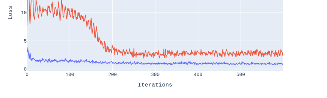
Figure 1: $\mathcal{E}(J_{\theta};\mathcal{B}_{\pi_{U}})$ (Error) and $\mathcal{E}(J_{\theta};\mathcal{B}_{\mathbb{P}})$ (Error P) determined w.r.t. a model trained on a uniform sampling scheme, i.e. samples were drawn from a uniform measure $\pi_{U}$ during training. Latter error was computed on a batch produced by the Euler-Mayurama scheme using the model’s policy. The $\mathcal{E}(J_{\theta};\mathcal{B}_{\mathbb{P}})$-error shows a high variance and poor convergence properties at a high magnitude. $\mathcal{E}(J_{\theta};\mathcal{B}_{\pi_{U}})$ converges to a value of $0.87$, $\mathcal{E}(J_{\theta};\mathcal{B}_{\mathbb{P}})$ oscillates between $3-4$ (Produced on Sznajd model as per Section LABEL:sec:evaluation).

The algorithm works as follows. Initially a batch is sampled from a distribution $\nu(\Omega)$. The time points $\{t_{i}\}_{i=1}^{N}$ are sampled uniformly or quasi-uniformly over $[0,T]$. The algorithm starts by sampling from the uncontrolled path space, i.e. with $\alpha=1$ and $\text{SDE}(t_{i},x,(1-\alpha)u),\;i=1,...,n$. From these fully-relaxed dynamics, the SDE is gradually introduced to the control signal. The variance of the control signal is rather high in the beginning. The rational is that the algorithm reduces the variance until a better approximation of the control function is available. After each propagation, the modulus is taken on the updated time as to maintain a uniform distribution over the time horizon. One sample is generated in $\mathcal{O}(N)$, for a batch size of $N$. The methodology is displayed in Algorithm 2. It is straightforward to transform the algorithm into an its off-policy version via the extension with a replay buffer. As seen in Figure 1 uniform sampling provides poor convergence in both the uniform $L^{2}$-norm and the $L^{2}$-norm with respect to an approximation of the law of the process.

Algorithm 2 Controlled Drift Relaxation

Input:
Batch size $N\in\mathbb{N}$,
Sample $(x,t,u)=\{(x_{i},t_{i},u_{i})\}_{i=1}^{N},x_{i}\in\mathbb{R}^{n},t_{i}\in[0,T]$, $u_{i}\in\mathcal{A}$
Learning rate $\beta$,
Initial distribution $\nu$,
Target measure $x_{d}$,
Relaxation coefficient $\alpha\in[0,1]$,
Stochastic Differential Equation SDE$(\cdot,\cdot,\cdot)$
Output: Sample $(x,t)$

  while $\alpha>0$ do

     for $i=1...N$ do

        $x^{\text{new}}_{i}\sim\nu(\Omega)$

        $x_{i}\leftarrow[t_{i}+\Delta t\leq T]\cdot\text{SDE}(t_{i},x_{i},(1-\alpha)u)+[t_{i}+\Delta t>T]\cdot x^{\text{new}}_{i}$

        $t_{i}\leftarrow(t_{i}+\Delta t)\mod T$

     end for

     $\alpha\leftarrow\alpha-\beta\nabla_{\alpha}(\alpha^{2}+\sum_{i=1...N}\frac{t_{i}}{TN}\mathcal{W}^{2}_{\Omega,2}(x_{i},x_{d}))$

     $\alpha\leftarrow\max(\min(\alpha,1),0)$

  end while