Dynamic Correlation Clustering in Sublinear Update Time

Abstract

We study the classic problem of correlation clustering in dynamic node streams. In this setting, nodes are either added or randomly deleted over time, and each node pair is connected by a positive or negative edge. The objective is to continuously find a partition which minimizes the sum of positive edges crossing clusters and negative edges within clusters. We present an algorithm that maintains an $O(1)$-approximation with $O(\operatorname{polylog}n)$ amortized update time. Prior to our work Behnezhad et al. ((2023b)) achieved a $5$-approximation with $O(1)$ expected update time in edge streams which translates in node streams to an $O(D)$-update time where $D$ is the maximum possible degree. Finally we complement our theoretical analysis with experiments on real world data.

1 Introduction

Clustering is a cornerstone of contemporary machine learning and data analysis. A successful clustering algorithm partitions data elements so that similar items reside within the same group, while dissimilar items are separated. Introduced in 2004 by Bansal, Blum and Chawla Bansal et al. ((2004)), the correlation clustering objective offers a natural approach to model this problem. Due to its concise and elegant formulation, this problem has drawn significant interest from researchers and practitioners, leading to applications across diverse domains. These include ensemble clustering identification ((Bonchi et al., 2013)), duplicate detection ((Arasu et al., 2009)), community mining ((Chen et al., 2012)), disambiguation tasks ((Kalashnikov et al., 2008)), automated labeling ((Agrawal et al., 2009, Chakrabarti et al., 2008)), and many more.

In the correlation clustering problem we are given a graph where each edge has either a positive or negative label, and where a positive edge $(u,v)$ indicates that $u,v$ are similar elements (and a negative edge $(u,v)$ indicates that $u,v$ are dissimilar), the objective is to compute a partition of the graph that minimizes the number of negative edges within clusters plus positive edges between clusters. Since the problem is NP-hard, researchers have focused on designing approximation algorithms.

The algorithm proposed by Cao et al. ((2024)) achieves an approximation ratio of $1.43+\varepsilon$, improving upon the previous $1.73+\varepsilon$ and $1.994+\varepsilon$ achieved by Cohen-Addad et al. ((2023, 2022b)). Prior to these developments, the best approximation guarantee of $2.06$ was attained by the algorithm of Chawla et al. ((2015)).

These above approaches are linear-programming-based: they require to solve a linear program and then provide a rounding algorithm. The best known “combinatorial” algorithm is due to a recent local search algorithm of Cohen-Addad et al. ((2024)) achieving a $1.845+\varepsilon$-approximation. Prior to this, the best known “combinatorial” algorithm was the celebrated pivot algorithm of Ailon et al. ((2008)) which consists in repeatedly creating a cluster by picking a random unclustered node, and clustering it with all its positive unclustered neighbors. The versatility of the scheme has led the pivot algorithm to be used in a variety of contexts, and in particular for designing dynamic algorithms Behnezhad et al. ((2019, 2022, 2023a)).

Dynamic algorithms hold a key position in algorithm design due to their relevance in handling real-world, evolving datasets. Consequently, substantial research has focused on crafting clustering algorithms expressly designed for dynamic environments (including streaming, online, and distributed settings) Lattanzi and Vassilvitskii ((2017)), Fichtenberger et al. ((2021)), Jaghargh et al. ((2019)), Cohen-Addad et al. ((2019)), Guo et al. ((2021)), Cohen-Addad et al. ((2022a)), Assadi and Wang ((2022)), Lattanzi et al. ((2021)), Behnezhad et al. ((2022, 2023a)), Bateni et al. ((2023)).

While the classical approach is to design variations of the Pivot algorithm of Ailon et al. ((2008)),  Cohen-Addad et al. ((2021)) provide an alternative approach based on a notion called agreement, which entails the calculation of the positive neighborhood similarity of pairs of nodes. While that approach is initially used in the context of distributed correlation clustering, it has been also used in Assadi and Wang ((2022)) to design a static algorithm with $n\operatorname{polylog}n$ time complexity. In the latter setting the algorithm does not read the entire input, otherwise a time complexity of $n\operatorname{polylog}n$ would be impossible for dense graphs. However the algorithm has access to the graph through queries. We formalize that model in 1 and ask the following natural question: in which settings can correlation clustering be solved in $o(n^{2})$ time?

Our Contribution

In this paper, our focus lies on the dynamic case, where nodes are inserted adversarially and / or deleted randomly over time. This setting has already been studied for other clustering problems in Epasto et al. ((2015)) and serves as a bridge between the fully adversarial and random input models. Our objective is to maintain an $O(1)$-approximate solution at any point in time, while paying as little computation time as possible upon modification of the input (node insertion or deletion). Unfortunately, the approximation algorithms mentioned above are computationally expensive and cannot be re-executed each time the input changes.

The best known bound for the fully dynamic setting is due to Behnezhad et al. ((2023a)) who provided a $5$-approximation in $O(m)$ total update time for adversarial edge insertions and deletions, where $m$ is the total number of positive edges of the graph. Of course, for node updates, the above approach can be used to achieve a $5$-approximation with $O(D)$ update time, where $D$ is the maximum positive degree of a node throughout the vertex sequence. Note that for dense graphs this is equivalent to a $\Theta(n^{2})$ algorithm. We ask whether it is possible to go beyond this bound if we are given indirect access to the graph through queries and we do not need to read the entire input.

We answer the above question positively. More precisely, we provide the first algorithm which achieves a constant factor approximation model with poly-logarithmic update time per node insertion/deletion . We also complement our theoretical result with experiments showing the effectiveness of our algorithm in practice.

2 Problem Definition and the Database Model of Computation

The disagreements minimization version of the correlation clustering problem receives as input a complete signed undirected graph $G=(V,E,s)$ where each edge $e=\{u,v\}$ is assigned a sign $s(e)\in\{\text{`}+\text{'},\text{`}-\text{'}\}$ and the goal is to find a partition of the nodes such that the number of $\text{`}-\text{'}$ edges inside the same cluster and $\text{`}+\text{'}$ edges in between clusters is minimized. For simplicity we denote the set of $\text{`}+\text{'}$ and $\text{`}-\text{'}$ edges by $E^{+}$ and $E^{-}$ respectively. A clustering is a partition of the nodes $\mathcal{C}=\{C_{1},C_{2},\dots,C_{k}\}$ and the cost of that clustering is ${|\{u,v\}\in E^{+}:u\in C_{i},v\in C_{j},i\neq j|}+{|\{u,v\}\in E^{-}:\exists i:u,v\in C_{i}|}$

Note that a complete undirected signed graph $G=(V,E,s)$ can be converted into a non-signed undirected graph $G=(V,E)$ where for each pair of nodes $\{u,v\}$ there is an edge between them in $G$ if and only if $s\left(\{u,v\}\right)=\text{`}+\text{'}$. Thus the absence of an edge between two nodes corresponds to a negative edge in the original signed graph and the presence of an edge to a positive edge in the original graph. For simplicity, throughout the paper we work with the non-signed equivalent definition of the correlation clustering problem.

The cost of a clustering $\mathcal{C}$ becomes:

$$|\{u,v\}\in E:u\in C_{i},v\in C_{j},i\neq j|+$$

$$|\{u,v\}\not\in E:\exists i:u,v\in C_{i}|$$

In our setting, nodes arrival are adversarial and node deletions are random. More precisely, at each time $t$ an adversary can decide either to add to the graph an adversarially chosen node or to delete a random node from the graph. Upon arrival a node reveals all the edges to previously arrived nodes and upon deletion all edges of the node are deleted. We denote by $u_{t}$ the node that arrived or left at time $t$ and by $G_{t}$ the graph structure after the first $t$ node arrivals/deletions. We also denote by $V_{t},E_{t}$ the set of nodes and edges of graph $G_{t}$ and by $n,m$ the total number of nodes and edges respectively that appeared throughout the dynamic stream. Note that $\forall t$ we have $|V_{t}|\leqslant n$ and $|E_{t}|\leqslant m$.

We denote by $OPT_{t}$ the cost of an optimal correlation clustering solution for graph $G_{t}$ and by $ALG_{t}$ the cost of a dynamic algorithm solution at time $t$. We say that an algorithm maintains a $c-$approximate solution if $\forall t$, input graphs and node streams we have $ALG_{t}\leqslant c\cdot OPT_{t}$.

We now formally define the computation model that we study in the paper. For an unsigned graph $G=(V,E)$ we denote by $V$, $E$ the set of nodes and edges respectively, and for a node $u\in V$ we use $N_{G}(u)$ to denote the neighborhood of $u$ in $G$. This model was considered by Assadi and Wang Assadi and Wang ((2022)) for designing sublinear algorithms for correlation clustering.

Definition 1 (Database model Assadi and Wang ((2022))).

Given a graph $G=(V,E)$ we have access to the graph structure through the following queries which have a cost of $O(\log|V|)$ :

1. Degree queries: $\forall u\in V$ we get its degree $|N_{G}(u)|$

2. Edge queries: $\forall u,v\in V$ we get whether $(u,v)\in E$

3. Neighborhood sample queries: $\forall u$, we get a node $v\in N_{G}(u)$ uniformly at random from set $N_{G}(u)$

Note that all these queries are easily implementable in the classical computational model where the graph is stored in the same processing unit as the one we use to compute our clustering solution. Thus, other than permitting us to avoid reading and storing the graph locally the Database model is strictly harder than the classical RAM computational model. Our goal is to maintain a constant approximation with respect to $OPT_{t}$ using only $\operatorname{polylog}n$ amortized update time (queries and computational operations). Note that for a dense graph this is sublinear in the time of reading the entire input sequence.

3 Algorithm and Techniques

Our approach draws inspiration from the Agreement algorithm, initially presented in Cohen-Addad et al. ((2021)). In particular, we leverage their key insight that to obtain a constant factor approximation it is enough to cluster together nodes with similar neighborhoods. Essentially, it is enough to focus on identifying near-clique structures. A second key idea that we use comes from Assadi and Wang ((2022)) where it is noted that to discover these dense substructures one does not need to examine the entire neighborhood of each node but it is possible to carefully sub-sample the edges of the graph to obtain a sparser structure. We build upon these two ideas along with developing several new techniques to obtain a constant factor approximation algorithm for dynamic graph with sublinear complexity.

The section is structured as follows: (1) we introduce the Agreement algorithm of Cohen-Addad et al. ((2021)) along with its useful properties; (2) we describe the challenges in applying that algorithm on a dynamic graph; (3) we describe a notification procedure which is the base of our algorithm; and (4) provide the pseudocode of our algorihtm.

3.1 The Agreement Algorithm

Before describing the Agreement algorithm of Cohen-Addad et al. ((2021)) we need to introduce two central notions to quantify the similarity between the neighborhood of two nodes.

Definition 2 (Agreement).

Two nodes $u,v$ are in $\varepsilon$-agreement in $G$ if

$$|N_{G}(u)\triangle N_{G}(v)|<\varepsilon\max\{|N_{G}(u)|,|N_{G}(v)|\}$$

where $\triangle$ denotes the symmetric difference of two sets.

Definition 3 (Heaviness).

A node is called $\varepsilon$-heavy if it is in $\varepsilon$-agreement with more than a $(1-\varepsilon)$-fraction of its neighbors. Otherwise it is called $\varepsilon$-light.

When $\varepsilon$ is clear from the context we will simply say that two nodes are or are not in agreement and that a node is heavy or light.

The Agreement algorithm uses the agreement and heaviness definitions to compute a solution to the correlation clustering problem, as described in Algorithm 1. We call the output of Algorithm 1 the agreement decomposition of the graph $G$.

Algorithm 1 AgreementAlgorithm($G$)

  Create a graph $\tilde{G}$ from $G$ by discarding all edges whose endpoints are not in $\varepsilon$-agreement.

  Discard all edges of $\tilde{G}$ between light nodes of $G$.

  Compute the connected components of $\tilde{G}$, and output them as the solution.

At a high level, the first two steps of Algorithm 1 can be characterized as a filtering procedure which ensures that two nodes with similar neighborhoods end up in the same connected component of $\tilde{G}$ and consequently in the same cluster of the final partitioning. The main lemma which helps bounding the approximation ratio of the Agreement algorithm and which will be also used to analyze the performance of our algorithm is the following:

Lemma 4 (rephrased from Cohen-Addad et al. ((2021))).

Let $\mathcal{C}=\{C_{1},C_{2},\dots,C_{k}\}$ be a clustering solution for graph $G=(V,E)$ and $\varepsilon$ a small enough constant. If the following properties hold:

1. $\forall i\in\{1,2,\dots,k\}$ and $u\in C_{i}$ such that $|C_{i}|>1$ we have $|N_{G}(u)\cap C_{i}|\geqslant\nicefrac{{3}}{{4}}|C_{i}|$

2. $\forall e=(u,v)\in E$ such that $u\in C_{i}$, $v\in C_{j}$ and $i\neq j$ then either $u$ and $v$ are not in $\varepsilon$-agreement or both nodes are not $\varepsilon$-heavy.

Then the cost of $\mathcal{C}$ is a constant factor approximation to that of the optimal correlation clustering solution for graph $G$

For $\varepsilon$ small enough Cohen-Addad et al. ((2021)) prove that Algorithm 1 satisfies both properties of 4 and therefore produces a constant factor approximation.

3.2 Challenges of Dynamic Agreement

Our goal is to design a dynamic version of the Agreement algorithm which consistently maintains a sparse graph $\tilde{G}$ whose induced clustering satisfy both conditions of 4 while only spending $O(\operatorname{polylog}n)$ update time upon node insertions and random deletions.

We briefly describe what are the main challenges that we face in such endeavour:

1. computing the agreement between two nodes or the heaviness of a node may take time $\Theta(n)$;

2. the number of agreement calculations performed by Algorithm 1 is equal to the number of edges in our graph; and

3. since the total complexity that we aim is $O(n\operatorname{polylog}n)$, the graph $\tilde{G}$ that we maintain should be both sparse at any point and stable (do not change significantly between consecutive times).

From a high level perspective, we solve those issues as follows. First, instead of computing exactly whether two nodes are in $\varepsilon$-agreement and whether a node is $\varepsilon$-heavy, we design two stochastic procedures, namely ProbabilisticAgreement($u,v,\varepsilon$) and Heavy($u,\varepsilon$), which only need a sample of logarithmic size of the two neighborhoods to answer correctly, with high probability, those questions. We defer the description of those procedures in Appendix E. Second, for each dense substructure, we maintain dynamically a random set of $O(\operatorname{polylog}n)$ heavy nodes. We call that sample the anchor set and show that the connections of those nodes are enough to recover a good clustering. Finally, to efficiently maintain our sparse graph $\tilde{G}$ we design a message-passing procedure, which we call $\mathrm{Notify}$, to communicate events across neighboring nodes. Roughly, this procedure propagates information about the arrival or deletion of a node $u$ to a $O(\operatorname{polylog}n)$-size randomly chosen subset of nodes within small hop distance from $u$. Whenever a node receives a “notification”, we either add, with some probability, this node to the anchor set and we revisit the agreement between that node and nodes already in the anchor set.

While similar ideas to resolve the first and second challenges have been already explored in the sublinear static algorithm of Assadi and Wang ((2022)) it is important to observe that applying the same principles in the dynamic sublinear setting is highly non-trivial. Indeed, in this setting it is not even clear if one can even maintain a good approximation of the degrees of nodes in sublinear time.

3.3 Notify Procedure

A central sub-procedure in our algorithm, which allow us to keep track of evolving clusters is the Notify procedure. We believe that it is of independent interest and we devote Section 3.3 entirely to its description. As mentioned before the Notify procedure is responsible to propagate the information of node arrivals and deletions to $O(\operatorname{polylog}n)$ nodes. We distinguish between different types of notifications depending on how many nodes did the notification propagate through from the “source” node that initiated the notify procedure.

Notifications are subdivided in categories depending on their type, which could be $\mathrm{Type}_{i},i=0,1,2$. A central definition in our algorithm and in its analysis is the “interesting event” definition.

Definition 5.

We say that $u$ participates in an “interesting event” either when $u$ arrives or $u$ receives a $\mathrm{Type}_{0}$ or $\mathrm{Type}_{1}$ notification.

To simplify the description of the algorithm. We denote by $d(u)$ the current degree of a node $u$ and we define the function $l(x)=\lfloor\log(x)\rfloor,\forall x>0$. With a slight abuse of notation for a node $u$ we denote by $l_{u}$ the quantity $l(d(u))$. Note that for all nodes $u$ we have that $2^{l_{u}}\leqslant d(u)<2^{l_{u}+1}$.

Each node $u$ stores sets $I^{0}_{u},I^{1}_{u},I^{2}_{u},\dots,I^{\log n}_{u}$ and $B^{0}_{u},B^{1}_{u},B^{2}_{u},\dots,B^{\log n}_{u}$. Set $I^{i}_{u}$ contains $u$’s last neighborhood sample when its degree was in $[2^{i},2^{i+1})$ and set $B^{i}_{u}$ contains all nodes $v$ such that $u\in I^{i}_{v}$.

Each time a node $u$ participates in an “interesting event” or receives a $\mathrm{Type}_{2}$ notification it stores a random sample of size $O(\log n)$ of its neighborhood in $I^{l_{u}}_{u}$. Further, $u$ enters the sets $B^{l_{u}}_{v}$ for all nodes $v\in I^{l_{u}}_{u}$ of its sample. Those nodes are responsible to notify $u$ when they get deleted. Thus, upon $u$’s deletion all nodes in $\bigcup_{i}B^{i}_{u}$ are notified.

This notification strategy has two key properties, that are: (1) $u$ gets notified and participates in an “interesting event” when a constant fraction of its neighborhood gets deleted; and (2) w.h.p. $u$ gets notified when its $2$-hop neighborhood changes substantially. Interestingly, the notification strategy does this while maintaining the expected complexity bounded by $O(\operatorname{polylog}n)$ each time the Notify procedure is called. Algorithm 2 contains the pseudocode of the notification procedure

Algorithm 2 Notify($u,\varepsilon$)

  if $u$ arrived then

     $I^{l_{u}}_{u}\xleftarrow{}$ sample $10^{10}\log n/\varepsilon$ random neighbors

     $\forall v\in I^{l_{u}}_{u}$: $B^{l_{u}}_{v}\xleftarrow{}B^{l_{u}}_{v}\cup\{u\}$

     $\forall v\in I^{l_{u}}_{u}$: $u$ sends $v$ a $\mathrm{Type}_{0}$ notification

  else if $u$ was deleted then

     $\forall v\in\bigcup_{i}B^{i}_{u}$: $u$ sends $v$ a $\mathrm{Type}_{0}$ notification

  end if

  for $i=0,1,2$ do

     for all $w$ that received a $\mathrm{Type}_{i}$ notification do

        $\forall v\in I^{l_{w}}_{w}$: $B^{l_{w}}_{v}\xleftarrow{}B^{l_{w}}_{v}\setminus\{w\}$

        $I^{l_{w}}_{w}\xleftarrow{}$ sample $10^{10}\log n/\varepsilon$ random neighbors

        $\forall v\in I^{l_{w}}_{w}$: $B^{l_{w}}_{v}\xleftarrow{}B^{l_{w}}_{v}\cup\{w\}$

        if $i\in\{0,1\}$ then

           $\forall v\in I^{l_{w}}_{w}$: $w$ sends $v$ a $\mathrm{Type}_{i+1}$ notification

        end if

     end for

  end for

3.4 Our Dynamic Algorithm Pseudocode

Our Algorithm 3 contains 4 procedures: the $\text{Notify}(v_{t},\varepsilon)$ procedure which we described in Section 3.3, the Clean($u,\varepsilon,t$) procedure, the Anchor($u,\varepsilon,t$) procedure and the Connect($u,\varepsilon,t$) procedure. Before describing the last three we introduce some auxiliary notation.

We denote by $\mathcal{I}_{t}$ the set of nodes that participated in an “interesting event” at round $t$. We also denote by $\Phi$ a dynamically changing (across the execution of our algorithm) subset of the nodes which we call anchor set. We avoid the subscript $t$ in the set $\Phi$ notation as it is always clear for the context at what time we are referring to. When a node $u$ is deleted, then, we also apply $\Phi\leftarrow\Phi\setminus\{u\}$. We maintain a sparse graph $\tilde{G_{t}}$ with the same node set of $G_{t}$ and with edge set $\tilde{E_{t}}\subseteq E_{t}$. We start our algorithm with $\tilde{G_{0}}$ being an empty graph. The backbone of our sparse solution $\tilde{G_{t}}$ is the anchor set nodes $\Phi$. Indeed, we have that $\forall e=(u,v)\in\tilde{E_{t}}$ either $u$ or $v$ are in $\Phi$. Moreover, for any node $u$ we denote by $\Phi_{u}$ the subset of the nodes in $\Phi$ connected to $u$ in our sparse solution $\tilde{G_{t}}$.

Algorithm 3 Dynamic Agreement (DA)

  on arrival/deletion of $v_{t}$ do

     $\text{Notify}(v_{t},\varepsilon)$

     for all $u\in\mathcal{I}_{t}$ do

        Clean($u,\varepsilon,t$)

        Anchor($u,\varepsilon,t$)

        Connect($u,\varepsilon,t$)

     end for

  end on

After the arrival or deletion of node $v_{t}$ and the propagation of notifications through the $\text{Notify}(v_{t},\varepsilon)$ procedure, for all nodes $u$ in an important event we do the following.

First we call the Clean($u,\varepsilon,t$) procedure which is responsible to delete edges between nodes which are not in $\varepsilon$-agreement anymore and delete from the anchor set nodes that lost too many edges in our sparse solution. These operations enable our algorithm to refine clusters which became too sparse or refine cluster assignment for nodes that are not anymore in $\varepsilon$-agreement.

Then we call the Anchor($u,\varepsilon,t$) where if $u$ is heavy then with probability $\min\{1,\frac{10^{7}\log n}{\varepsilon|N_{G_{t}}(u)|}\}$ we add this node to $\Phi$. If $u$ is added in $\Phi$ then we calculate agreements with all of its neighbors and whenever $u$ is in agreement with a neighbor $v$ we add edge $(u,v)$ to our sparse solution $\tilde{G_{t}}$. As mentioned previously the anchor nodes are representative nodes of clusters. Thus, the Anchor($u,\varepsilon,t$) procedure allows us to update the set of anchor nodes so that they behave approximately like a uniform sample of each cluster.

Finally, we initiate the Connect procedure. The purpose of this step is to add some redundant information so that the clustering is stable and also ensure that nodes that are inserted lately are guaranteed to be connected to some anchor node of their cluster.

Algorithm 4 Connect($u,\varepsilon,t$)

  Let $J_{u}$ be a random sample of size $\nicefrac{{10^{5}\log n}}{{\varepsilon}}$ from $N_{G_{t}}(u)$.

  for $w\in J_{u}$ do

     for $r\in\Phi_{w}$ do

        If $r$ is heavy and in agreement with $u$ then add the edge $(r,w)$ to $\tilde{G_{t}}$

     end for

  end for

Algorithm 5 Anchor($u,\varepsilon,t$)

  $X_{u}\sim\text{Bernoulli}(\min\{\nicefrac{{10^{7}\log n}}{{\varepsilon|N_{G_{t}}(u)|}},1\})$

  if $u\in\Phi$ then

     Delete all edges $(u,v)$ where $v\not\in\Phi$ from $\tilde{G_{t}}$

  end if

  if $u$ is heavy in $G_{t}$ and $X_{u}=1$ then

     For every neighbor $v$, if $u$ and $v$ are in agreement add edge $(u,v)$ in our sparse solution $\tilde{G_{t}}$.

  end if

  if $X_{u}=1$ then

     Add $u$ to $\Phi$ at the end of iteration $t$

  else if $u\in\Phi$ and $X_{u}=0$ then

     Delete $u$ from $\Phi$ at the end of iteration $t$

  end if

Algorithm 6 Clean($u,\varepsilon,t$)

  for $w\in\Phi_{u}$ do

     if $w$ not in agreement with $u$ or $w$ is not heavy then

        Delete edge $(w,u)$ from $\tilde{G_{t}}$

     end if

     if $w$ lost more than an $\varepsilon$ fraction of its edges in $\tilde{G_{t}}$ from when it entered $\Phi$ then

        Delete $w$ from $\Phi$ and all edges between $w$ and its neighbors in $\tilde{G_{t}}$

     end if

  end for

4 Overview of our Analysis

In this section we give a high level description of our proof strategy, the full proof is available in the Appendix. We first present the high-level ideas on how to prove 6 and then we bound the running time.

Theorem 6.

For each time $t$ the Dynamic Agreement algorithm outputs an $O(1)-$approximate clustering with probability at least $1-5/n$.

4.1 Overview of the Correctness Proof

To prove the correctness of our algorithm we show that at any time $t$: 1) for every cluster $C$ that is identified by the offline Agreement algorithm (which is known to be constant factor approximate) our algorithm w.h.p. forms a cluster that is a superset of $C$, and 2) every cluster $C^{\prime}$ detected by our algorithm is a dense cluster w.h.p., meaning that $\forall u\in C^{\prime}$, $|N_{G_{t}}(u)\cap C^{\prime}|\geqslant(1-c^{\prime}\cdot\varepsilon)|C^{\prime}|$ for small enough $\varepsilon$, and a constant $c^{\prime}\ll 1/\varepsilon$. Combining the above two facts and union bounding over all time $t$, we get that all clusters detected by the offline agreement algorithm are found, and all detected clusters are very dense. So using the fact that the offline agreement algorithm is a constant approximation algorithm we can show that also our algorithm is. The formal proof of the two facts requires the introduction of several concepts and probabilistic events, and is deferred to Appendix A and Appendix B. Here we give a high-level overview of our proof strategy. For the remainder of this section, we call a cluster computed by the offline agreement algorithm a good cluster.

All good clusters are detected.

As discussed in Section 3 the key idea of the algorithm is to design a sampling strategy and a notify procedure to keep track of the good clusters efficiently. The key idea is to not identify a good cluster only at the time that is formed, but to design a strategy to track the most important events that affect any node in the graph during the execution of the algorithm and to maintain the clustering structure through connections to the anchor set nodes.

Let a cluster $C$ be a good cluster at time $t$. In our analysis, we analyze the last $\frac{\varepsilon}{c}|C|$ interesting events involving nodes of cluster $C$. Let $L\subset C$ be the set of nodes involved in these last interesting events, we further subdivide $L$ into $L_{1}$ containing the half of $L$ that participated earlier in interesting events, and $L_{2}$ containing those that participated later. We also denote $R=C\setminus L$. Intuitively we show that every node connects to another node in the anchor set either in the first or second part of our analysis.

Let $t_{u}$ be the last time in which a node $u\in L$ participates in an “interesting event”. Our notification procedure ensures that w.h.p. $u$’s neighborhood does not change significantly after its last participation in an “interesting event”, i.e., $N_{G_{t_{u}}}(u)\simeq N_{G_{t^{\prime}}}(u)$, $\forall t^{\prime}\in[t_{u},t]$ (see 14 and the preceding discussion). At the same time, we know that at time $t$, $u$ belongs to the good cluster $C$ and by the properties of the agreement decomposition (see Appendix G) we have that $N_{G_{t}}(u)\simeq C$. Combining the last two observations we can conclude that $N_{G_{t_{u}}}(u)\simeq C$. This line of arguments can be extended to all nodes $v\in N_{G_{t_{u}}}(u)\cap R$ which by the definition of $R$ do not participate in an “interesting event” after time $t_{u}$. Thus, $\forall v\in N_{G_{t_{u}}}(u)\cap R$, it holds that: $N_{G_{t_{u}}}(v)\simeq C$. In addition, $R$ contains almost all nodes of $C$, thus $N_{G_{t_{u}}}(u)\cap R\simeq C$. Combining all these observations we can conclude that $u$ is in agreement with almost all of its neighbors at time $t_{u}$, and therefore it is heavy. In addition, if $u$ enters in the anchor set, it remains there until time $t$. This is proved in 17 of Appendix A.

We are ready to prove that our algorithm finds a cluster $C^{\prime}\supseteq C$ at time $t$ for every good cluster $C$ detected by the offline agreement algorithm. As described in Section 3, the clusters that our algorithms form are determined by the connected components in our sparse solution graph $\tilde{G}_{t}$. To this end we argue that each node of $C$ is connected to a node in $C$ that is in the anchor set in $\tilde{G}_{t}$. We show how this is true for each of the three sets $R,L_{1},L_{2}$. For $R$ we recall that each node in $L_{1}\subset L$ is heavy and enters the anchor set with probability $O(\frac{\log n}{\varepsilon|N_{G_{t_{u}}}(u)|})$ at time $t_{u}$.

Given that $|L_{1}|=\frac{c}{2\varepsilon}|C|$ for $c\ll\varepsilon$, we can show that each $v\in R$ has a neighbor $v^{\prime}\in L_{1}$ that enters the anchor set w.h.p., and $v^{\prime}$ connects to $v$ in $\tilde{G}_{t}$ during the $Anchor(v^{\prime},\varepsilon,t_{v^{\prime}})$ procedure. This is formally proved in 20 of Appendix A. Similarly, each node in $L_{1}$ has a neighbor in $L_{2}$ that enters the anchor set w.h.p.. Finally, we prove that each node $v$ in $L_{2}$ is connected to a node $v^{\prime}$ in the anchor set in $L_{1}$ w.h.p.. In fact, since most pairs of nodes in $L_{1}\cup L_{2}$ are in agreement w.h.p. there are many common neighbors $w\in R$ such that $w$ is in agreement with both $v^{\prime}$ and $v$, which implies that the $Connect(v,\varepsilon,t_{v})$ will connect $v$ to $v^{\prime}$. See 22 of Appendix A for the formal proof. Hence, all nodes in $C$ get connected to a node in the anchor set (which as we claimed above remains in the anchor set until time $t$). To conclude the argument we also note that the nodes in the anchor set are connected to each other because they share most of their neighbors. This is proved in 23 of Appendix A.

All found clusters are good.

To prove that all clusters identified by our algorithm are good clusters, we follow a proof strategy similarly to Cohen-Addad et al. ((2021)). Roughly speaking, we show that each connected component $C^{\prime}$ of $\tilde{G}_{t}$ has diameter $4$, which follows by observing that all nodes in the anchor set are within distance $2$ from each other, and that each other node is connected to a node in the anchor set. Then, due to the transitivity of the agreement property, it follows that all nodes in the connected component $C^{\prime}$ are in agreement with each other. This last claim, then further implies that for each $v\in C^{\prime}$ it holds that $|N_{G_{t}}\cap C^{\prime}|\geqslant(1-c\varepsilon)|C^{\prime}|$ which makes $C^{\prime}$ a good cluster. See Appendix B for the formal proof.

4.2 Overview of Running Time Bound

We observe that our algorithm is correct even when deletions occur adversarially, but this unfortunately does not hold for the analysis of its running time. Notice that for insertions the running time is bounded by the $O(\operatorname{polylog}n)$ forward notifications sent as a result of the insertion of a new node. On the other hand, the deletion of a node $u$ may cause all nodes in $\bigcup_{i}B^{i}_{u}$ to receive a notification, and this in turn causes those nodes to send forward notifications. The issue arises in that there is no bound in the size of $|\bigcup_{i}B^{i}_{u}|$ when deletions occur adversarially. In fact, we can construct an instance where $|\bigcup_{i}B^{i}_{u}|\in\widetilde{\Theta}(n)$ for $\widetilde{O}(n)$ many deletions. Thankfully, in the case where the deletions appear in a random order, this cannot happen as we can nicely bound the expectation of $|\bigcup_{i}B^{i}_{u}|$ to be $O(\operatorname{polylog}n)$ for a node $u$ chosen uniformly at random. We devote Appendix C in the formal proof of the running time analysis.

5 Experimental Evaluation

We conduct two sets of experiments. We first evaluate the performance of our algorithm to the same set of real-world graphs that were used in Lattanzi et al. ((2021)). Then, we investigate how the running time of our algorithm scales with the size of the input.

5.1 Baselines and Datasets

We compare our algorithm to Singletons where its output always consists of only singleton clusters and Pivot-Dynamic Behnezhad et al. ((2023a)) which is a dynamic variation of the Pivot algorithm Ailon et al. ((2008)) for edge streams with $O(1)$ update time. While Pivot-Dynamic guarantees a constant factor approximation, Singletons does not have any theoretical guarantees. Nevertheless, it has been observed in Lattanzi et al. ((2021)) that sparse graphs tend to not have a good correlation clustering structure, and often the clustering that consists of only singleton clusters is a competitive solution.

We consider five real-world datasets. For the first set of experiments, we use four graphs from SNAP Leskovec and Krevl ((2014)) that include a Social network (musae-facebook), an email network (email-Enron), a collaboration network (ca-AstroPh), and a paper citation network (cit-HepTh).

In the second set of experiments where we investigate the runtime of our algorithm with respect to the size of the input we use Drift Vergara et al. ((2012)), Rodriguez-Lujan et al. ((2014)) from the UCI Machine Learning Repository Dua and Graff ((2017)). The dataset contains $13,910$ points embedded in a space of $129$ dimensions. Each point corresponds to a node in our graph and we add a positive connection between two nodes if the euclidean distance of the corresponding points is below a certain threshold. The lower we set that threshold the denser the graph becomes.

All graphs are formatted so as to be undirected and without parallel edges. In addition, we create the node streams of node additions and deletions as follows: we first create a random arrival sequence for all the nodes. Subsequently in between any two additions, with probability $p$, we select at random a node of the current graph and delete it. If all nodes have already arrived then at each time we randomly select one of those and delete it.

5.2 Setup and Experimental Details

Our code is written in Python 3.11.5 and is available at https://github.com/andreasr27/DCC. We set the deletion probability in between any two node arrivals to be $0.2$. The agreement parameter is set to $\varepsilon=0.2$, as this setting exhibited the best behavior in Cohen-Addad et al. ((2021)) and Lattanzi et al. ((2021)).

In addition, we set the number of samples in our procedures to a small constant. More precisely, all our subroutines use a random sample of size $2$ and the probability of a node joining the anchor set is set to $20/d_{u}$ where $d_{u}$ denotes its degree in the current graph. Here we deviate from the numbers we use in theory as we observe that, in practice, for sparse graphs only running time is affected. We note that in the runtime calculation we do not include reading the input and calculating the quality of our clustering. We do this in an effort to best approximate the Database model in 1 while reading the input we implement suitable data structures where the graph is stored in the form of adjacency lists which permit node additions, deletions and getting a random sample in $O(1)$ expected time.

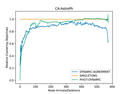
Figure 1: Correlation clustering objective relative to singletons

Solution quality.

In the first set of experiments we run all three algorithms and plot their performance relative to Singletons, that is, we plot the cost of solution produced by our algorithm or Pivot-Dynamic divided by the cost of the solution of Singletons. In all datasets, Dynamic-Agreement consistently outperforms both Pivot-Dynamic and Singletons. For example, in Fig. 1 we plot the correlation clustering objective every $10$ nodes additions/deletions in the node stream. We observe that after a constant fraction of all nodes have arrived, the clustering objective of our algorithm relative to Singletons remains stable both for node additions and deletions. On the contrary the performance of Pivot-Dynamic fluctuates and tends to increase especially in the last part of the sequence when all nodes have already arrived and the node stream contains predominantly deletions. A similar behaviour is observed in the other three datasets which are deferred to Appendix H. In Appendix H we also present a table which gives an estimate of the optimum offline solution based on the classical Pivot algorithm of Ailon et al. ((2008)). In Table 1 we see that our algorithm is slower to the Pivot-Dynamic implementation. This is something that we expect since Pivot-Dynamic is extremely efficient for sparse graphs.

	DA	PD
musae-facebook	2.27	0.1
email-Enron	2.79	0.12
cit-HepTh	3.84	0.21
ca-AstroPh	2.96	0.11

Table 1: Runtimes of the algorithms Dynamic-Agreement (DA) and Pivot-Dynamic (PD).

	Relative Objective		Running Time
Density	DA	PD	DA	PD
253.36	0.696	0.610	12.48	0.28
114.87	0.605	0.551	14.54	0.16
69.74	0.522	0.504	15.82	0.11
52.17	0.389	0.416	14.10	0.09
42.25	0.320	0.375	12.85	0.07

Table 2: Summary of our scalability experiment for the algorithms Dynamic-Agreement (DA) and Pivot-Dynamic (PD), on the Drift dataset at varying densities.

Running time.

As mentioned previously, we constructed a graph using the Drift dataset by associating points with nodes and adding positive edges between nodes if the Euclidean distance of the corresponding points is less than a threshold. Different thresholds lead to the creation of distinct graphs. Now we relate the density of the graph (average node degree) with the runtimes and clustering quality of both Dynamic-Agreement and Pivot-Dynamic. Table 2 shows the average relative clustering quality of each algorithm over the entire node stream and their running times.

We observe that both Dynamic-Agreement and Pivot-Dynamic outperform Singletons, as expected, since Singletons excels in sparse graphs and offers poor quality solutions in denser graphs. Additionally, the running time of Dynamic-Agreement remains stable when the density of the graphs increases confirming that the algorithm’s running time is not affected by the graph density. On the other hand, the running time of Pivot-Dynamic increases linearly with the density. This suggests that for very large and dense graphs, where even reading the entire input is prohibitive Dynamic-Agreement scales smoothly, further validating the theory.

Experimental summary.

We observe that the newly proposed algorithm computes high quality solutions for both sparse and dense graphs. This is in contrast with comparison methods that fail to produce good solutions in at least one of the two settings. We also show that even if the runtime of our algorithm is higher compared to the competitor, its runtime does not increase with the density of the input graph. This is inline with our theoretical results and is achieved via our sampling and notify strategies.

Conclusion and Future Work

We provide the first sublinear time algorithm for correlation clustering in dynamic streams where nodes are added adversarially and deleted randomly. Our algorithm is based on new and carefully defined sampling and notification strategies that can be of independent interest. We also show experimentally that our algorithm provides high quality solution both for dense and sparse graph outperforming previously known algorithms.

A very interesting open question is to extend our result in the general setting where both nodes’ addition and deletion is adversarial. One possible way of achieving the later would be to use a different sparse-dense decomposition which is more stable and requires less updates so that it is maintained approximately, e.g., the one proposed by Assadi and Wang ((2022)).

Reducing the amortize update time in our setting is another very interesting and natural question.

Appendix A Finding Dense Clusters

In this section we prove that our algorithm correctly finds the non-singleton clusters of $G_{t}$ that are also found by the AgreementAlgorithm($G_{t}$) when the agreement and heaviness parameters are set to a small enough value. That is, let $C$ be a non-singleton cluster that is found by AgreementAlgorithm($G_{t_{current}}$) at time $t_{current}$ when the agreement and heaviness parameters are set to $\nicefrac{{\varepsilon}}{{10^{14}}}$. It can be proven that cluster $C$ is extremely dense, i.e., it forms almost a clique, with very few outgoing edges. In 23 we prove that at time $t_{current}$ our algorithm outputs a cluster $C^{\prime}$ that contains all nodes of $C$, i.e., $C^{\prime}\supseteq C$. While the latter may not seem surprising per se (note that a trivial algorithm which clusters all nodes in the same partition also achieves that property), our approach consists in a delicate argument where we prove that for all non-trivial clusters $C$ found by AgreementAlgorithm($G_{t_{current}}$) our algorithm always constructs a cluster $C^{\prime}\supseteq C$ and at the same time in Appendix B all clusters $C^{\prime}$ constructed by our algorithm (which may not be constructed by AgreementAlgorithm($G_{t_{current}}$)) are very dense. In order to simplify the notation we use $t_{c}$ instead of $t_{current}$ in our formulas.

The first challenge in the current section is to prove that the notify procedure correctly samples enough nodes of $C$, “close enough” to time $t_{current}$, so that many of these nodes enter the anchor set and help us reconstruct $C$. Note that the latter ensures that enough nodes from a specific cluster enter the anchor set, but does not ensure that these clusters are correctly found. Indeed, the last arriving node may not enter the anchor set and at the same time the “interesting events” that its arrival generates may not induce any node to join the anchor set. However, to get a constant factor approximation, we still need to ensure that the last node of $C$ is clustered correctly with the rest of the cluster. In order to ensure the latter, our algorithm uses the Connect($v,\varepsilon$) procedure. Connect($v,\varepsilon$) constructs a sample of $v$’s neighborhood and for every node $w$ in that sample, it checks whether $v$ is in $\varepsilon$-agreement with any node $r\in\Phi_{w}$, i.e., any node that is in the anchor set of and if so $v$ is connected to $r$.

In the current section we make great use of the relation between $C$ and $N_{G_{t_{c}}}(u)$ for a node $u\in C$, indeed since $C$ is a dense cluster found by AgreementAlgorithm($G_{t_{current}}$) at time $t_{current}$, informally we have that $N_{G_{t_{c}}}(u)\approx C$ (see the properties of the Agreement decomposition in Appendix G).

Consider the last $\lfloor\nicefrac{{\varepsilon}}{{10^{4}}}|C|\rfloor$ nodes of $C$ that participate in an “interesting event” and denote those nodes by $u_{i}$ for $i=1,2,\dots,\lfloor\nicefrac{{\varepsilon}}{{10^{4}}}|C|\rfloor$. For each $u_{i}$ denote by $t_{i}$ the last time that this node participated in an “interesting event”, so that $t_{1}\leqslant t_{2}\leqslant\dots\leqslant t_{\lfloor\nicefrac{{\varepsilon}}{{10^{4}}}|C|\rfloor}$. If two nodes $u_{i},u_{j}$ participated in an “interesting event” after the same arrival or deletion in the node streams then we order with respect to the type of notification received, that is, $t_{i}\leqslant t_{j}$ if $u_{i}$ just arrived or received a notification of a lower type than $u_{j}$. Ties are broken arbitrarily but consistently. Note that both nodes $u_{i}$ and times $t_{i}$ for $i=1,2,\dots,\lfloor\nicefrac{{\varepsilon}}{{10^{4}}}|C|\rfloor$ are random variables which depend on the internal randomness of the Notify procedure.

We now introduce some auxiliary notation:

1. $L=\{u_{1},u_{2},\dots,u_{\lfloor\nicefrac{{\varepsilon}}{{10^{4}}}|C|\rfloor}\}$ and $R=C\setminus L$.

2. $L_{1}=\{u_{1},u_{2},\dots,u_{\lfloor\nicefrac{{\varepsilon}}{{2\cdot 10^{4}}}|C|\rfloor}\}$.

3. $L_{2}=\{u_{\lfloor\nicefrac{{\varepsilon}}{{2\cdot 10^{4}}}|C|\rfloor+1},u_{\lfloor\nicefrac{{\varepsilon}}{{2\cdot 10^{4}}}|C|\rfloor+2},\dots,u_{\lfloor\nicefrac{{\varepsilon}}{{10^{4}}}|C|\rfloor}\}$.

4. $L^{i}=\{u_{1},u_{2},\dots,u_{i}\}$.

5. We denote as $t^{\prime}$ the earliest time that all nodes of $R$ have arrived.

Again, note that since the $u_{i}$’s and $t_{i}$’s are random variables then also $R,L,L_{1},L_{2},L^{i}$ and $t^{\prime}$ are random variables.

We start by some simple observations where we argue that after time $t^{\prime}$ all nodes of $C$ that have already arrived form a dense subgraph.

Observation 7.

$\forall u\in C$ we have:

$$(1-\varepsilon/10^{13})|C|\leqslant|N_{G_{t_{c}}}(u)|\leqslant(1+\varepsilon/10^{13})|C|$$

Proof.

From Property 6 and Property 10 in Appendix G the result is immediate. ∎

Observation 8.

$\forall u\in C$ we have:

$$|N_{G_{t_{c}}}(u)\cap C|\geqslant(1-\varepsilon/10^{13})|C|$$

Proof.

Follows immediately from  Property 4. ∎

Observation 9.

For each $u\in C$ that arrived at time $t\in[t^{\prime},t_{c}]$ we have:

$$|N_{G_{t}}(u)|\geqslant|N_{G_{t}}(u)\cap C|\geqslant(1-2\varepsilon/10^{4})|C|$$

Proof.

The left-hand side inequality is obvious. For the right inequality note that at time $t^{\prime}$ all nodes in $R$ have arrived. Thus,

$$|N_{G_{t}}(u)\cap C| \geqslant|N_{G_{t_{c}}}(u)\cap C|-|L|\geqslant(1-\varepsilon/10^{13})|C|-\varepsilon/10^{4}|C|$$

$$\geqslant(1-2\varepsilon/10^{4})|C|$$

Where in the second inequality we use 8 and $|L|=\lfloor\varepsilon/10^{4}|C|\rfloor$. ∎

Observation 10.

For each $u\in C$ that has already arrived before time $t\in[t^{\prime},t_{c}]$ we have:

$$|C\setminus N_{G_{t}}(u)|\leqslant 2\varepsilon/10^{4}|C|\leqslant\varepsilon/10^{3}|N_{G_{t}}(u)|$$

Proof.

The left inequality is immediate from 9 and the second one holds for $\varepsilon$ small enough again using 9. ∎

10 informally states that the neighborhood of any node $v\in C$ between times $t^{\prime}$ and $t_{c}$ contains $C$ almost in its entirety. Let $t\in[t^{\prime},t_{c}]$ be a time when node $v$ has already arrived, then we have that: $N_{G_{t}}(v)\supseteq C^{\prime}$ and $C^{\prime}\simeq C$. Ideally, we would like all nodes $v\in C$ to have almost their final neighborhood between times $t^{\prime}$ and $t_{c}$ so that the Anchor procedure correctly reconstructs the cluster $C$. That is, we would like to also have $N_{G_{t}}(v)\subseteq C^{\prime\prime}$ and $C^{\prime\prime}\simeq C$. While the latter may be not true in general, we prove that with high probability at every time $t_{i}$ it is true for $u_{i}$ and a large part of its neighborhood.

We introduce auxiliary notation to formalize these claims.

Definition 11.

For a node $v\in C$ and time $t$ we define the following events:

$$M_{v}^{t} =\{|N_{G_{t}}(v)\setminus N_{G_{t_{c}}}(v)|<\nicefrac{{\varepsilon}}{{8\cdot 10^{4}}}|N_{G_{t}}(v)|\}$$

$$A_{v}^{t} =\left\{\left\{v\in\mathcal{I}_{t}\right\}\lor\left\{v\text{ received a }Type_{2}\text{ notification at time }t\right\}\right\}$$

$M_{v}^{t}$ is true if at least a $(1-\nicefrac{{\varepsilon}}{{8\cdot 10^{4}}})$ fraction of $v$’s neighborhood at time $t$ does not get deleted until time $t_{c}$. Also, note that if $A_{v}^{t}$ is true then $v$ samples with replacement $10^{10}\log n/\varepsilon$ neighbors at time $t$. By $\overline{M_{v}^{t}}$ and $\overline{A_{v}^{t}}$ we denote the complementary events of ${M_{v}^{t}}$ and ${A_{v}^{t}}$ respectively.

The rest of the section is devoted in arguing that with high probability at each time $t_{i}$, both $u_{i}$ and nearly all its neighbors possess almost their “final” neighborhood. The crux of our analysis is based on the following two observations (stated informally for the moment). For all $v\in R\cup L_{i}$: (1) If $M_{v}^{t_{i}}$ is true, then $N_{G_{t_{i}}}(v)\simeq C$; and (2) The event $\overline{M_{v}^{t_{i}}}\land A_{v}^{t_{i}}$ happens with low probability.

In the following lemma we prove structural properties of the neighborhood $N_{G_{t_{i}}}(v)$ of a node when $v$ when $M_{v}^{t_{i}}$ is true.

Lemma 12.

$\forall v\in R\cup L^{i}$ we have that if $M_{v}^{t_{i}}$ is true then:

$$|N_{G_{t_{i}}}(v)|<(1+\nicefrac{{\varepsilon}}{{2\cdot 10^{4}}})|C|$$ (1)

$$|N_{G_{t_{i}}}(v)\setminus C|<\nicefrac{{\varepsilon}}{{10^{4}}}|C|<\nicefrac{{\varepsilon}}{{10^{3}}}|N_{G_{t_{i}}}(v)|$$ (2)

Proof.

1. For the first statement we prove the contrapositive, i.e., we argue that $|N_{G_{t_{i}}}(v)|\geqslant(1+\nicefrac{{\varepsilon}}{{2\cdot 10^{4}}})|C|$ implies $\overline{M_{v}^{t_{i}}}$. We distinguish between the cases:

   • $|N_{G_{t_{i}}}(v)|\geqslant\frac{|N_{G_{t_{c}}}(v)|}{(1-\varepsilon/(8\cdot 10^{4}))}$, then

     $$|N_{G_{t_{i}}}(v)\setminus N_{G_{t_{c}}}(v)| \geqslant|N_{G_{t_{i}}}(v)|-|N_{G_{t_{c}}}(v)|$$

     $$\geqslant\varepsilon/(8\cdot 10^{4})|N_{G_{t_{i}}}(v)|$$

   • $|N_{G_{t_{i}}}(v)|<\frac{|N_{G_{t_{c}}}(v)|}{(1-\varepsilon/(8\cdot 10^{4}))}$, in that case from 7 we have the bound $|N_{G_{t_{c}}}(v)|\leqslant(1+\varepsilon/10^{13})|C|$

     $$|N_{G_{t_{i}}}(v)\setminus N_{G_{t_{c}}}(v)|$$

     $$\geqslant|N_{G_{t_{i}}}(v)|-|N_{G_{t_{c}}}(v)|$$

     $$\geqslant(1+\varepsilon/(2\cdot 10^{4}))|C|-|N_{G_{t_{c}}}(v)|$$

     $$\geqslant\left(\frac{1+\varepsilon/(2\cdot 10^{4})}{1+\varepsilon/10^{13}}-1\right)|N_{G_{t_{c}}}(v)|$$

     $$\geqslant\left(\frac{1+\varepsilon/(2\cdot 10^{4})}{1+\varepsilon/10^{13}}-1\right)\left(1-\varepsilon/(8\cdot 10^{4})\right)|N_{G_{t_{i}}}(v)|$$

     $$\geqslant\left(\varepsilon/(2\cdot 10^{4})-\varepsilon/10^{13}\right)\left(\frac{1-\varepsilon/(8\cdot 10^{4})}{1+\varepsilon/10^{13}}\right)|N_{G_{t_{i}}}(v)|$$

     $$\geqslant\varepsilon/(8\cdot 10^{4})|N_{G_{t_{i}}}(v)|$$

     Where in the second inequality we used our assumption that $|N_{G_{t_{i}}}(v)|\geqslant(1+\nicefrac{{\varepsilon}}{{2\cdot 10^{4}}})|C|$, the third one from 7, the fourth one from the fact that we are in the second case and the last one holds for $\varepsilon$ small enough.

2. From the first part of the current lemma we have that $|N_{G_{t_{i}}}(v)|<(1+\nicefrac{{\varepsilon}}{{2\cdot 10^{4}}})|C|$ and from 9 we have that $|N_{G_{t_{i}}}(v)\cap C|\geqslant(1-2\varepsilon/10^{4})|C|$, consequently:

   $$|N_{G_{t_{i}}}(v)\setminus C| =|N_{G_{t_{i}}}(v)|-|N_{G_{t_{i}}}(v)\cap C|$$

   $$<(1+\varepsilon/(2\cdot 10^{4}))|C|-(1-2\varepsilon/10^{4})|C|$$

   $$<3\varepsilon/10^{4}|C|$$

   $$<3\varepsilon/10^{4}\frac{|N_{G_{t_{i}}}(v)|}{(1-2\varepsilon/10^{4})}$$

   $$<\varepsilon/10^{3}|N_{G_{t_{i}}}(v)|$$

   Where the second inequality holds for $\varepsilon$ small enough and proves the first inequality of (2) in the current lemma, the third inequality uses again 9 and the last inequality holds for $\varepsilon$ small enough.

∎

By Combining 12 and 10 we can argue that $\forall v\in R\cup L^{i}$ if $M_{v}^{t_{i}}$ is true then $N_{G_{t_{i}}}(v)\simeq C$. Consequently for two neighboring nodes $v,u\in R\cup L^{i}$: $M_{v}^{t_{i}}\land M_{u}^{t_{i}}$ implies that $N_{G_{t_{i}}}(v)\simeq N_{G_{t_{i}}}(u)\simeq C$ and consequently $u$ and $v$ are in agreement. We formalize the latter in the following lemma.

Lemma 13.

For all neighboring nodes $v,u\in R\cup L^{i}$: if $M_{v}^{t_{i}}\land M_{u}^{t_{i}}$ is true then $v$ and $u$ are in $\varepsilon/10$-agreement.

Proof.

Since both $M_{u}^{t_{i}}$ and $M_{v}^{t_{i}}$ are true, from 12 we have that:

$$|N_{G_{t_{i}}}(u)\setminus C|<\varepsilon/10^{3}|N_{G_{t_{i}}}(u)|$$

and

$$|N_{G_{t_{i}}}(v)\setminus C|<\varepsilon/10^{3}|N_{G_{t_{i}}}(v)|$$

Also from 10 it holds that:

$$|C\setminus N_{G_{t_{i}}}(u)|\leqslant\varepsilon/10^{3}|N_{G_{t_{i}}}(u)|$$

and

$$|C\setminus N_{G_{t_{i}}}(v)|\leqslant\varepsilon/10^{3}|N_{G_{t_{i}}}(v)|$$

To argue that $|N_{G_{t_{i}}}(u)\triangle N_{G_{t_{i}}}(v)|\leqslant\varepsilon/10\max\{|N_{G_{t_{i}}}(u)|,N_{G_{t_{i}}}(v)|\}$, we bound both $|N_{G_{t_{i}}}(u)\setminus N_{G_{t_{i}}}(v)|$ and $|N_{G_{t_{i}}}(v)\setminus N_{G_{t_{i}}}(u)|$ by $\varepsilon/10^{2}\max\{|N_{G_{t_{i}}}(u_{i})|,N_{G_{t_{i}}}(w)|\}$. From the latter the lemma follows since $2\varepsilon/10^{2}<\varepsilon/10$ for $\varepsilon$ small enough. We upper bound the size of $N_{G_{t_{i}}}(u)\setminus N_{G_{t_{i}}}(v)$:

$$|N_{G_{t_{i}}}(u)\setminus N_{G_{t_{i}}}(v)| \leqslant|N_{G_{t_{i}}}(u)\setminus C|+|C\setminus N_{G_{t_{i}}}(v)|$$

$$\leqslant\varepsilon/10^{3}|N_{G_{t_{i}}}(u)|+\varepsilon/10^{3}|N_{G_{t_{i}}}(v)|$$

$$\leqslant\varepsilon/10^{2}\max\{|N_{G_{t_{i}}}(u)|,N_{G_{t_{i}}}(v)|\}$$

and the upper bound of $|N_{G_{t_{i}}}(v)\setminus N_{G_{t_{i}}}(u)|$ follows the same line of arguments. ∎

We know prove that the probability of a node $v\in R\cup L_{i}$ both sampling its neighborhood at time $t_{i}$ and having a neighborhood which is very different than $C$ is very low. The following lemma is crucial, as it subsequently help us argue that most of the neighboring nodes of $u_{i}$ at time $t_{i}$ have almost their final neighborhoods.

Lemma 14.

$\forall v\in C$ and time $t$ we have that:

$${\bf Pr}[\overline{M_{v}^{t}}\land A_{v}^{t}\land\{v\in R\cup L^{i}\}\land\{t\geqslant t_{i}\}]<1/n^{10^{4}}$$

Proof.

Let $d_{t^{\prime}}$ denote the degree of node $v$ at time $t^{\prime}$ and $l_{t^{\prime}}=l(d_{t^{\prime}})$. In this proof we write $I_{v,t^{\prime}}$ to denote the neighborhood sample stored in $I^{l_{t}}_{v}$ at time $t^{\prime}$. Note that $I_{v,t^{\prime}}$ and $I_{v,t^{\prime\prime}}$ for $t^{\prime}<t^{\prime\prime}$ may be different if for example $v$ received a $\mathrm{Type}_{2}$ notification between those times and updated its neighborhood sample.

Also, for all $w\in N_{G_{t}}(v)\setminus N_{G_{t_{c}}}(v)$ let $t_{w}$ be the time when $w$ gets deleted from the node stream and let $w_{j}$ be the $j$-th element to be deleted in $N_{G_{t}}(v)\setminus N_{G_{t_{c}}}(v)$. For $j=1,2,\dots,|N_{G_{t}}(v)\setminus N_{G_{t_{c}}}(v)|$, we define event $E_{j}=\left\{w_{j}\not\in I_{v,t_{w}}\right\}$.

We argue that $\{v\in R\cup L^{i}\}\land\{t\geqslant t_{i}\}$ implies $\bigcap\limits_{1\leqslant j\leqslant|N_{G_{t}}(v)\setminus N_{G_{t_{c}}}(v)|}E_{j}$. Indeed, $\overline{E_{j}}$ implies that $v\in B^{l_{t}}_{w}$ at time $t_{w}$. Consequently, upon its deletion, $w$ would send a $\mathrm{Type}_{0}$ notification to $v$ and $v$ would participate in an “interesting event” between times $[t_{i}+1,t_{c})$. The latter implies that $v\not\in R\cup L_{i}$.

Thus:

$${\bf Pr}[\overline{M_{v}^{t}}\land A_{v}^{t}\land\{v\in R\cup L^{i}\}\land\{t\geqslant t_{i}\}] \leqslant{\bf Pr}[\overline{M_{v}^{t}}\land A_{v}^{t}\land\bigcap\limits_{1\leqslant j\leqslant|N_{G_{t}}(v)\setminus N_{G_{t_{c}}}(v)|}E_{j}]$$

$$\leqslant{\bf Pr}[A_{v}^{t}\land\bigcap\limits_{1\leqslant j\leqslant\nicefrac{{\varepsilon}}{{8\cdot 10^{4}}}d_{t}}E_{j}]$$

$$=\prod_{1\leqslant j\leqslant\nicefrac{{\varepsilon}}{{8\cdot 10^{4}}}d_{t}}{\bf Pr}[A_{v}^{t}\land E_{j}\mid\bigcap\limits_{j^{\prime}<j}\{A_{v}^{t}\land E_{j^{\prime}}\}]$$

where in the second inequality we used that $|N_{G_{t}}(v)\setminus N_{G_{t_{c}}}(v)|\geqslant\nicefrac{{\varepsilon}}{{8\cdot 10^{4}}}|N_{G_{t}}(v)|$. Note that since:

$$\left(1-\nicefrac{{1}}{{2\cdot d_{t}}}\right)^{\left(\nicefrac{{10^{10}\log n}}{{\varepsilon}}\right)\cdot\left(\nicefrac{{\varepsilon}}{{8\cdot 10^{4}}}d_{t}\right)}<1/n^{10^{4}}$$

It is enough to argue that:

$${\bf Pr}[A_{v}^{t}\land E_{j}\mid\bigcap\limits_{j^{\prime}<j}\{A_{v}^{t}\land E_{j^{\prime}}\}]<(1-\nicefrac{{1}}{{2\cdot d_{t}}})^{10^{10}\log n/\varepsilon}$$

Let $\tilde{t}_{w_{j^{\prime}}},j^{\prime}<j$, be the random variable denoting the last time before $t_{w_{j^{\prime}}}$ that $I^{l_{t}}_{v}$ was updated. Since $t<t_{w_{j}}$:

1. $A_{v}^{t}$ implies that:

   1. $t\leqslant\tilde{t}_{w_{j}}<t_{w_{j}}$; and

   2. $w_{j}\in N_{G_{\tilde{t}_{w_{j}}}}(v)$

2. By the definition of $\tilde{t}_{w_{j}}$: $|N_{G_{\tilde{t}_{w_{j}}}}(v)|<2\cdot d_{t}$

Let $r_{i}$ be the $i$-th random sample used to construct $I^{l_{t}}_{v}$ at time $t_{w}$, i.e., $I_{w_{j},t_{w_{j}}}$. By the principle of deferred decisions it is enough to decide whether $r_{i}$ is equal to $w_{j}$ at time $t_{w_{j}}$. Note that given $\bigcap\limits_{j^{\prime}<j}\{A_{v}^{t}\land E_{j^{\prime}}\}$, $r_{i}$ is a uniform at random sample from a set that contains $w_{j}$ and has at most $2\cdot d_{t}$ elements, i.e., set $N_{G_{\tilde{t}_{w_{j}}}}(v)\setminus\bigcup_{j^{\prime}<j}w_{j^{\prime}}$. Thus:

$${\bf Pr}[\left\{r_{i}=v\right\}\mid\bigcap\limits_{j^{\prime}<j}\{A_{v}^{t}\land E_{j^{\prime}}\}\}]\leqslant(1-\nicefrac{{1}}{{2\cdot d_{t}}})$$

and the proof is concluded by noting that $I_{w_{j},t_{w_{j}}}=\bigcup\limits_{i\leqslant 10^{10}\log n/\varepsilon}{r_{i}}$ and $r_{i}$’s are independent. ∎

As already mentioned, we prove that for time $t_{i}$ most of $u_{i}$’s neighboring nodes have almost their final neighborhood. Towards that goal, for every $t_{i}$ we define a random set which contains all neighboring nodes of $u_{i}$ whose neighborhood at time $t_{i}$ is “very” different from their final one.

Definition 15.

For $t_{i}$ we define the random set: $D_{t_{i}}=\{v:v\in N_{G_{t_{i}}}(u_{i})\cap(R\cup L^{i})\land\overline{M_{v}^{t_{i}}}\}$.

We prove that the size of this random set is small with high probability.

Lemma 16.

$\forall t_{i}$ we have that:

$${\bf Pr}[|D_{t_{i}}|\geqslant\varepsilon/10^{5}|N_{G_{t_{i}}}(u_{i})|]<1/n^{10^{3}}$$

Proof.

In this proof when we write $I_{u_{i}}$ we refer to $u_{i}$’s neighborhood sample constructed via the connect procedure at that specific time $t_{i}$. Note that:

$${\bf Pr}[|D_{t_{i}}|\geqslant\varepsilon/10^{5}|N_{G_{t_{i}}}(u_{i})|] ={\bf Pr}[\{|D_{t_{i}}|\geqslant\varepsilon/10^{5}|N_{G_{t_{i}}}(u_{i})|\}\land\{D_{t_{i}}\cap I_{u_{i}}=\emptyset\}]$$

$$+{\bf Pr}[\{|D_{t_{i}}|\geqslant\varepsilon/10^{5}|N_{G_{t_{i}}}(u_{i})|\}\land\{D_{t_{i}}\cap I_{u_{i}}\neq\emptyset\}]$$

We bound each of the two terms in the right hand side independently.

For the first term we have:

$${\bf Pr}[\{|D_{t_{i}}|\geqslant\varepsilon/10^{5}|N_{G_{t_{i}}}(u_{i})|\}\land\{D_{t_{i}}\cap I_{u_{i}}=\emptyset\}] \leqslant(1-\varepsilon/10^{5})^{10^{10}\log n/\varepsilon}$$

$$\leqslant 1/n^{10^{5}}$$

since $N_{G_{t_{i}}}(u_{i})\setminus D_{t_{i}}$ is at least a $(1-\varepsilon/10^{5})$ fraction of $N_{G_{t_{i}}}(u_{i})$.

For the second term we have:

$${\bf Pr}[\{|D_{t_{i}}|\geqslant\varepsilon/10^{5}|N_{G_{t_{i}}}(u_{i})|\}\land\{D_{t_{i}}\cap I_{u_{i}}\neq\emptyset\}] =\sum_{v\in C}{\bf Pr}[\{v\in N_{G_{t_{i}}}(u_{i})\}\land\{v\in D_{t_{i}}\}\land\{v\in I_{u_{i}}\}]$$

$$\leqslant\sum_{v\in C}{\bf Pr}[\{v\in N_{G_{t_{i}}}(u_{i})\}\land\{v\in D_{t_{i}}\}\land\{v\in A_{v}^{t_{i}}\}]$$

$$\leqslant\sum_{v\in C}{\bf Pr}[\{v\in D_{t_{i}}\}\land A_{v}^{t_{i}}]$$

$$\leqslant\sum_{v\in C}{\bf Pr}[\{v\in R\cup L^{i}\}\land\{\overline{M_{v}^{t_{i}}}\}\land A_{v}^{t_{i}}]$$

$$\leqslant n\cdot(1/n^{10^{4}})$$

$$\leqslant 1/n^{10^{4}-1}$$

Where in the first inequality note that $v\in I_{u_{i}}$ implies $A_{v}^{t_{i}}$ (since $v$ receives a notification from $u_{i}$), in the second inequality we used that $D_{t_{i}}\subseteq N_{G_{t_{i}}}(u_{i})$, in the third inequality we used the definition of set $D_{t_{i}}$ and in the fourth inequality we used 14.

Combining the two upper bounds concludes the proof. ∎

The next lemma argues that if $D_{t_{i}}$ is small and $N_{G_{t_{i}}}(u_{i})\simeq C$ then $u_{i}$ is heavy at time $t_{i}$.

Theorem 17.

If $\{|D_{t_{i}}|<\varepsilon/10^{5}|N_{G_{t_{i}}}(u_{i})|\}\land M_{u_{i}}^{t_{i}}$ is true then $u_{i}$ is $\varepsilon/10$-heavy at time $t_{i}$. In addition, if $u_{i}$ also enters the anchor set at time $t_{i}$ then it remains in it at least until time $t_{c}$.

Proof.

By the definition of $D_{t_{i}}$ we have that $\forall w\in N_{G_{t_{i}}}(u_{i})\cap(R\cup L^{i})\setminus D_{t_{i}}$ the event $M_{w}^{t_{i}}$ is true. Thus, since $M_{u_{i}}^{t_{i}}$ is also true from 13 we can conclude that $u_{i}$ and $w$ are in $\varepsilon/10$-agreement.

We now argue that $u_{i}$ is in $\varepsilon/10$ agreement with at least a $1-\varepsilon/10$ fraction of its neighborhood at time $t_{i}$. For this, note that:

$$|N_{G_{t_{i}}}(u_{i})\setminus\left(N_{G_{t_{i}}}(u_{i})\cap(R\cup L^{i})\setminus D_{t_{i}}\right)| \leqslant|N_{G_{t_{i}}}(u_{i})\setminus\left(N_{G_{t_{i}}}(u_{i})\cap(R\cup L^{i})\right)|+|D_{t_{i}}|$$

$$=|N_{G_{t_{i}}}(u_{i})\setminus(R\cup L^{i})|+|D_{t_{i}}|$$

$$\leqslant|N_{G_{t_{i}}}(u_{i})\setminus C|+|C\setminus(R\cup L^{i})|+|D_{t_{i}}|$$

$$\leqslant|N_{G_{t_{i}}}(u_{i})\setminus C|+|C\setminus R|+|D_{t_{i}}|$$

$$=|N_{G_{t_{i}}}(u_{i})\setminus C|+|L|+|D_{t_{i}}|$$

$$\leqslant\varepsilon/10^{3}|N_{G_{t_{i}}}(u_{i})|+\varepsilon/10^{4}|C|+|D_{t_{i}}|$$

$$\leqslant\varepsilon/10^{3}|N_{G_{t_{i}}}(u_{i})|+5\varepsilon/10^{4}|N_{G_{t_{i}}}(u_{i})|+|D_{t_{i}}|$$

$$\leqslant\varepsilon/10^{3}|N_{G_{t_{i}}}(u_{i})|+5\varepsilon/10^{4}|N_{G_{t_{i}}}(u_{i})|+\varepsilon/10^{5}|N_{G_{t_{i}}}(u_{i})|$$

$$\leqslant\varepsilon/10|N_{G_{t_{i}}}(u_{i})|$$

Where in the sixth inequality we used (2) of 12 (since $M_{u_{i}}^{t_{i}}$ is true), in the seventh inequality we used that $|D_{t_{i}}|<\varepsilon/10^{5}|N_{G_{t_{i}}}(u_{i})|$ and the last inequality holds for $\varepsilon$ small enough.

To prove the second claim of the theorem, we note that if $u_{i}$ enters the anchor set at time $t_{i}$ then to exit that set before time $t_{c}$ at least an $\varepsilon$-fraction of its neighborhood at time $t_{i}$ needs to call the $Clean(\cdot,\varepsilon)$ procedure and consequently participate in an “interesting event”. That is, for $\varepsilon$ small enough, at least $\varepsilon(1-\varepsilon/10)|N_{G_{t_{i}}}(u_{i})|\geqslant\varepsilon/2|N_{G_{t_{i}}}(u_{i})|$ nodes in $N_{G_{t_{i}}}(u_{i})$ need to participate in an “interesting event”. However, such nodes can be at most:

$$|N_{G_{t_{i}}}(u_{i})\setminus C|+|L\setminus(R\cup L^{i})| \leqslant|N_{G_{t_{i}}}(u_{i})\setminus C|+|L|$$

$$\leqslant\varepsilon/10^{3}|N_{G_{t_{i}}}(u_{i})|+\varepsilon/10^{4}|C|$$

$$\leqslant\varepsilon/10^{3}|N_{G_{t_{i}}}(u_{i})|+\varepsilon/10^{3}|N_{G_{t_{i}}}(u_{i})|$$

$$\leqslant 2\cdot\varepsilon/10^{3}|N_{G_{t_{i}}}(u_{i})|$$

which is smaller than $\varepsilon/2|N_{G_{t_{i}}}(u_{i})|$. In the second inequality we used the cardinality of $L$ and in the third inequality we used (2) of 12. ∎

Note that $A_{u_{i}}^{t_{i}}$ is always true from the definition of $u_{i}$ and $t_{i}$. Combining 14 and 16 we deduce that event $\{|D_{t_{i}}|<\varepsilon/10^{5}|N_{G_{t_{i}}}(u_{i})|\}\land M_{u_{i}}^{t_{i}}$ happens with high probability. Thus, from 17 we conclude that $u_{i}$ is $\varepsilon/10$-heavy at time $t_{i}$ with high probability.

The proof proceeds arguing that the following events happen with high probability:

• For every node $v\in R$ there exists a node $u_{i}\in L_{1}$ such that: (1) $u_{i}$ enters the anchor set at time $t_{i}$; (2) $u_{i}$ is in agreement with node $v$ at time $t_{i}$; and (3) $u_{i}$ does not exit the anchor set before time $t_{c}$. Consequently edge $(u_{i},v)$ is added to our sparse solution graph $\tilde{G_{t_{i}}}$ and remains in our sparse solution at least until time $t_{c}$.

• Similarly, we argue that for every node $v\in L_{1}$ there exists a node $u_{i}\in L_{2}$ such that (1), (2) and (3) hold. So that edge $(u_{i},v)$ is added to our sparse solution graph $\tilde{G_{t_{i}}}$ and remains in our sparse solution at least until time $t_{c}$.

• The last part of the proof argues how the Connect($\cdot,\varepsilon$) procedure clusters nodes in $L_{2}$ that do not enter the anchor set with the rest of $C$. At time $t_{i}$ when $u_{i}\in L_{2}$ participates in an “interesting event” most nodes in $R$ have their neighborhood similar to their final, i.e., at time $t_{c}$, neighborhood, consequently they are in agreement with $u_{i}$. In addition to that, $u_{i}$ is in agreement with almost all nodes in $L_{1}$, therefore there are many triangles of the form $u_{i},v,w$ where $v\in R$, $w\in\Phi_{v}\cap L_{1}$ and all three nodes are in agreement. The Connect($u_{i},\varepsilon$) connects $u_{i}$ to the rest of the cluster with high probability using the edge $(u_{i},w)$ in one of those triangles.

To prove the aforementioned points, we define the following random set:

Definition 18.

For $v\in C$ we define the random set:

$$T_{v}=\left\{i\in\{1,2,\dots,\lfloor\varepsilon/10^{4}|C|\rfloor\}:\overline{M_{v}^{t_{i}}}\land\{(u_{i},v)\in E_{t_{i}}\}\right\}$$

For a node $v\in C$, Definition 18 captures which times during the last $\lfloor\varepsilon/10^{4}|C|\rfloor$ “interesting events”, node $v$ was connected to $u_{i}$ and its neighborhood was different from its final one. We proceed by proving that for every node in $v\in R\cup L_{1}$, $|T_{v}|$ is small with high probability.

Lemma 19.

Let $v\in R\cup L_{1}$, then

$${\bf Pr}[|T_{v}|\geqslant\varepsilon/10^{5}|C|]<1/n^{10^{2}}$$

Proof.

In this proof, for a node $u_{i}\in L$ when we write $I_{u_{i}}$ we refer to $u_{i}$’s neighborhood sample constructed via the connect procedure at time $t_{i}$. For short we write $\left[\varepsilon/10^{4}|C|\right]$ instead of $\{1,2,\dots,\lfloor\varepsilon/10^{4}|C|\rfloor\}$. We first argue that event $\bigcap_{i\in\left[\varepsilon/10^{4}|C|\right]}M_{u_{i}}^{t_{i}}$ happens with high probability.

$${\bf Pr}[\bigcap_{i\in\left[\varepsilon/10^{4}|C|\right]}M_{u_{i}}^{t_{i}}] =1-{\bf Pr}[\exists i\in\left[\varepsilon/10^{4}|C|\right]:\overline{M_{u_{i}}^{t_{i}}}]$$

$$\geqslant 1-\sum_{i\in\left[\varepsilon/10^{4}|C|\right]}{\bf Pr}[\overline{M_{u_{i}}^{t_{i}}}]$$

$$\geqslant 1-\sum_{i\in\left[\varepsilon/10^{4}|C|\right]}{\bf Pr}[\overline{M_{u_{i}}^{t_{i}}}\land A_{u_{i}}^{t_{i}}]$$

$$\geqslant 1-n\cdot 1/n^{10^{4}}$$

$$\geqslant 1-1/n^{10^{3}}$$

where in the first inequality we used the union bound, in the second inequality we used that $A_{u_{i}}^{t_{i}}$ is always true by definition of $u_{i}$ and $t_{i}$ and in the third inequality we used 14. Thus using

$${\bf Pr}[|T_{v}|\geqslant\varepsilon/10^{5}|C|] ={\bf Pr}[\{|T_{v}|\geqslant\varepsilon/10^{5}|C|\}\land\bigcap_{i\in\left[\varepsilon/10^{4}|C|\right]}M_{u_{i}}^{t_{i}}]+{\bf Pr}[\{|T_{v}|\geqslant\varepsilon/10^{5}|C|\}\land\overline{\bigcap_{i\in\left[\varepsilon/10^{4}|C|\right]}M_{u_{i}}^{t_{i}}}]$$

$$\leqslant{\bf Pr}[\{|T_{v}|\geqslant\varepsilon/10^{5}|C|\}\land\bigcap_{i\in\left[\varepsilon/10^{4}|C|\right]}M_{u_{i}}^{t_{i}}]+1/n^{10^{3}}$$

We focus on upper bounding the first term of the right hand side. Again, using the law of total probability we have that:

$${\bf Pr}[\{|T_{v}|\geqslant\varepsilon/10^{5}|C|\}\land\bigcap_{i\in\left[\varepsilon/10^{4}|C|\right]}M_{u_{i}}^{t_{i}}] ={\bf Pr}[\{|T_{v}|\geqslant\varepsilon/10^{5}|C|\}\land\bigcap_{i\in\left[\varepsilon/10^{4}|C|\right]}M_{u_{i}}^{t_{i}}\land\{\forall i\in T_{v}\;v\not\in I_{u_{i}}\}]$$

$$+{\bf Pr}[\{|T_{v}|\geqslant\varepsilon/10^{5}|C|\}\land\bigcap_{i\in\left[\varepsilon/10^{4}|C|\right]}M_{u_{i}}^{t_{i}}\land\{\exists i\in T_{v}:\;v\in I_{u_{i}}\}]$$

For the first term note that for $\varepsilon$ small enough and using (1) of 12 we have that: if $\bigcap_{i\in\left[\varepsilon/10^{4}|C|\right]}M_{u_{i}}^{t_{i}}$ is true then $\forall i\in\left[\varepsilon/10^{4}|C|\right]$ we have that $|N_{G_{t_{i}}}(u_{i})|<2|C|$. Now consider the following random process: each time our algorithm samples $u_{i}$’s neighborhood to create $I_{u_{i}}$ we sample uniformly at random the set $N_{G_{t_{i}}}(u_{i})\cup\{r_{|N_{G_{t_{i}}}(u_{i})|+1},r_{|N_{G_{t_{i}}}(u_{i})|+2},\dots,r_{2|C|}\}$ to create sets $\tilde{I}_{u_{i}}$ where $r_{j}$ nodes only exist for analysis purposes. Now note that:

$${\bf Pr}[\{|T_{v}|\geqslant\varepsilon/10^{5}|C|\}\land\bigcap_{i\in\left[\varepsilon/10^{4}|C|\right]}M_{u_{i}}^{t_{i}}\land\{\forall i\in T_{v}:\;v\not\in I_{u_{i}}\}]\leqslant$$

$${\bf Pr}[\{|T_{v}|\geqslant\varepsilon/10^{5}|C|\}\land\bigcap_{i\in\left[\varepsilon/10^{4}|C|\right]}M_{u_{i}}^{t_{i}}\land\{\forall i\in T_{v}:\;v\not\in\tilde{I}_{u_{i}}\}]\leqslant$$

$$\left(1-1/(2|C|)\right)^{(10^{10}\log n/\varepsilon)\cdot(\varepsilon/10^{5}|C|)}\leqslant$$

$$\left(1-1/(2|C|)\right)^{10^{5}\log n|C|}\leqslant$$

$$(1/n)^{10^{5}/2}\leqslant$$

$$1/n^{10^{4}}$$

We continue by upper bounding ${\bf Pr}[\{|T_{v}|\geqslant\varepsilon/10^{5}|C|\}\land\bigcap_{i\in\left[\varepsilon/10^{4}|C|\right]}M_{u_{i}}^{t_{i}}\land\{\exists i\in T_{v}:\;v\in I_{u_{i}}\}]$ as follows:

$${\bf Pr}[\{|T_{v}|\geqslant\varepsilon/10^{5}|C|\}\land\bigcap_{i\in\left[\varepsilon/10^{4}|C|\right]}M_{u_{i}}^{t_{i}}\land\{\exists i\in T_{v}:\;v\in I_{u_{i}}\}] \leqslant\sum_{i\in\{1,2,\dots,\varepsilon/10^{4}|C|\}}{\bf Pr}[i\in T_{v},v\in I_{u_{i}}]$$

$$\leqslant\sum_{i\in\{1,2,\dots,\varepsilon/10^{4}|C|\}}{\bf Pr}[\tilde{M_{v}^{t_{i}}}\land A_{v}^{t_{i}}]$$

$$\leqslant n\cdot(1/n^{10^{4}})$$

$$\leqslant 1/n^{10^{4}-1}$$

Where in the first inequality we used the union bound, in the second inequality we used the fact that event $\{v\in I_{u_{i}}\}$ implies $A_{v}^{t_{i}}$, and in the third one we used 14.

The proof follows by noting that $1/n^{10^{3}}+1/n^{10^{4}}+1/n^{10^{4}-1}<1/n^{10^{2}}$ ∎

We continue proving that, with high probability, every node in $R$ is selected by a node in $L_{1}$ which enters the anchor set and remains in the anchor set until at least time $t_{c}$.

Lemma 20.

For every node $v\in R$ let

$$X_{v}=\left\{\exists i\in[\varepsilon/(2\cdot 10^{4})|C|]:\{u_{i}\in L_{1}\text{ enters the anchor set }\}\land\{(v,u_{i})\in E_{t_{i^{\prime}}},\forall i^{\prime}\in[i,t_{c}]\right\}$$

then ${\bf Pr}[X_{v}]>1-1/n^{10}$.

Proof.

Let $i\in\{1,2,\dots,\lfloor\varepsilon/(2\cdot 10^{4})|C|\rfloor\}$ be such that $\{|D_{t_{i}}|<\varepsilon/10^{5}|N_{G_{t_{i}}}(u_{i})|\}\land{M_{v}^{t_{i}}}\land{M_{u_{i}}^{t_{i}}}\land\{(u_{i},v)\in E_{t_{i}}\}$ is true, we then know from 17 that if $u_{i}$ enters the anchor set at that time $t_{i}$, edge $(u_{i},v)$ is added to our sparse solution and remains in it at least until time $t_{c}$. Thus, it is useful to define the following set:

$$Y_{v}=\left\{i\in\{1,2,\dots,\lfloor\varepsilon/(2\cdot 10^{4})|C|\rfloor:\;\{|D_{t_{i}}|<\varepsilon/10^{5}|N_{G_{t_{i}}}(u_{i})|\}\land{M_{v}^{t_{i}}}\land{M_{u_{i}}^{t_{i}}}\land\{(u_{i},v)\in E_{t_{i}}\}\right\}$$

We proceed by proving that with high probability $|Y_{v}|$ is “large”.

Note that from 8 we have that:

$$|\left\{i\in\{1,2,\dots,\lfloor\varepsilon/(2\cdot 10^{4})|C|\rfloor:\;(u_{i},v)\in E_{t_{i}}\right\}|\geqslant\varepsilon/(2\cdot 10^{4})|C|-\varepsilon/10^{13}|C|>\varepsilon/(3\cdot 10^{4})|C|$$

where the second inequality holds for $\varepsilon$ small enough.

For simplicity let:

$$\mathcal{R}=\bigcap_{i\in\left[\varepsilon/(2\cdot 10^{4})|C|\right]}\left\{\{|D_{t_{i}}|<\varepsilon/10^{5}|N_{G_{t_{i}}}(u_{i})|\}\land M_{u_{i}}^{t_{i}}\right\}\land\{|T_{v}|<\varepsilon/10^{5}|C|\}$$

Note that $\mathcal{R}$ implies that:

$$|Y_{v}|\geqslant\varepsilon/(3\cdot 10^{4})|C|-\varepsilon/10^{5}|C|>\varepsilon/(4\cdot 10^{4})|C|$$

where the second inequality holds for $\varepsilon$ small enough. We continue upper bounding the probability that $\mathcal{R}$ does not occur as follows:

$${\bf Pr}[\overline{\mathcal{R}}]\leqslant \sum_{i\in\left[\varepsilon/(2\cdot 10^{4})|C|\right]}{\bf Pr}[\{|D_{t_{i}}|\geqslant\varepsilon/10^{5}|N_{G_{t_{i}}}(u_{i})|\}]$$

$$+\sum_{i\in\left[\varepsilon/(2\cdot 10^{4})|C|\right]}{\bf Pr}[\overline{M_{u_{i}}^{t_{i}}}]$$

$$+{\bf Pr}[\{|T_{v}|\geqslant\varepsilon/10^{5}|C|\}]$$

$$\leqslant n\cdot(1/n^{10^{4}})+n\cdot(1/n^{10^{3}})+1/n^{10^{2}}$$

$$\leqslant 3/n^{10^{2}}$$

where in the first inequality we use the union bound and in the second we use 14, 16 and 19.

Note that $\mathcal{R}$ also implies that $u_{i}$ enters the anchor set at time $t_{i}$ with probability at least $\min\{\nicefrac{{10^{7}\log n}}{{2\varepsilon|C|}},1\}$ where we used (1) in 12 for $\varepsilon$ small enough. In addition, note that under any realization of the random variables $|N_{G_{t_{1}}}(u_{1})|,|N_{G_{t_{2}}}(u_{2})|,\dots$ the randomness of the Anchor procedure is independent from the randomness of the Connect procedure. Consequently:

$${\bf Pr}[\overline{X_{v}}] ={\bf Pr}\overline{[X_{v}}\cap\overline{\mathcal{R}}]+{\bf Pr}[\overline{X_{v}}\cap\mathcal{R}]$$

$$\leqslant{\bf Pr}[\overline{\mathcal{R}}]+{\bf Pr}[\overline{X_{v}}\cap\mathcal{R}]$$

$$\leqslant 3/n^{10^{2}}+{\bf Pr}[\overline{X_{v}}\cap\mathcal{R}]$$

$$\leqslant 3/n^{10^{2}}+{\bf Pr}[\overline{X_{v}}\cap\{|Y_{v}|>\varepsilon/(4\cdot 10^{4})|C|\}]$$

$$\leqslant 3/n^{10^{2}}+(1-\min\{\nicefrac{{10^{7}\log n}}{{2\varepsilon|C|}},1\})^{\varepsilon/(4\cdot 10^{4})|C|}$$

$$\leqslant 3/n^{10^{2}}+1/n^{10^{2}}$$

$$<1/n^{10}$$

∎

Using the same line of arguments as 20 in 21 we argue that every node in $L_{1}$ is selected by a node in $L_{2}$ which enters the anchor set and remains in the anchor set until at least time $t_{c}$. We state the lemma and omit the proof.

Lemma 21.

For every node $v\in L_{1}$ let

$$X_{v}=\left\{\exists i\in\{\varepsilon/(2\cdot 10^{4})|C|+1,\dots,\varepsilon/10^{4}|C|\}]:\{u_{i}\in L_{2}\text{ enters the anchor set }\}\land\{(v,u_{i})\in E_{t_{i^{\prime}}},\forall i^{\prime}\in[i,t_{c}]\right\}$$

then ${\bf Pr}[X_{v}]>1-1/n^{10}$.

Proof.

Omitted as it follows the same line of reasoning with the proof of 20. ∎

We underline that while the essence of both 20 and 21 could be summarized in a single lemma, in the last part of this section we use the facts that 20 refers to how nodes in $R$ get into the cluster through nodes in $L_{1}$ and 21 refers to how nodes in $L_{1}$ get into the cluster through nodes in $L_{2}$.

The last part of the section is devoted in arguing that through the Connect($\cdot,\varepsilon$) procedure, with high probability, all nodes in $L_{2}$ get connected to some node in $L_{1}$ in our sparse solution.

Lemma 22.

For every node $u_{j}\in L_{2}$ let

$$X_{u_{j}}=\left\{\exists i\in[\varepsilon/(2\cdot 10^{4})|C|]:\{u_{i}\in L_{1}\text{ enters the anchor set }\}\land\{(u_{j},u_{i})\in E_{t_{i^{\prime}}},\forall i^{\prime}\in[t_{j},t_{c}]\right\}$$

then

$${\bf Pr}[X_{u_{j}}]\geqslant 1-1/n^{10}$$

Proof.

The proof proceeds by arguing that:

1. $u_{j}$ is connected to almost all nodes $R$;

2. let $w\in R$, then $N_{G_{t_{j}}}(u_{j})\cap N_{G_{t_{j}}}(w)\cap L_{1}$ is a sufficiently large fraction of $L_{1}$;

3. with high probability almost all nodes in $N_{G_{t_{j}}}(u_{j})\cap N_{G_{t_{j}}}(w)\cap L_{1}$ have almost their final neighborhood; and

4. with high probability one of those nodes is in the anchor set.

It is useful to define the following event:

$$\mathcal{R}=\bigcap_{i\in\left[\varepsilon/(2\cdot 10^{4})|C|\right]}\left\{\{|D_{t_{i}}|<\varepsilon/10^{5}|N_{G_{t_{i}}}(u_{i})|\}\land M_{u_{i}}^{t_{i}}\right\}$$

We upper bound the probability that $\mathcal{R}$ does not occur as follows:

$${\bf Pr}[\overline{\mathcal{R}}]\leqslant \sum_{i\in\left[\varepsilon/(2\cdot 10^{4})|C|\right]}{\bf Pr}[\{|D_{t_{i}}|\geqslant\varepsilon/10^{5}|N_{G_{t_{i}}}(u_{i})|\}]$$

$$+\sum_{i\in\left[\varepsilon/(2\cdot 10^{4})|C|\right]}{\bf Pr}[\overline{M_{u_{i}}^{t_{i}}}]$$

$$\leqslant n\cdot(1/n^{10^{4}})+n\cdot(1/n^{10^{3}})$$

$$\leqslant 1/n^{10^{2}}$$

where in the first inequality we use the union bound and in the second we use 14 and 16.

Let $w\in N_{G_{t_{j}}}(u_{j})\cap R$, from 7 we have that:

$$|N_{G_{t_{j}}}(u_{j})\cap N_{G_{t_{j}}}(w)\cap L_{1}| \geqslant|L_{1}|-\varepsilon/10^{13}|C|-\varepsilon/10^{13}|C|$$

$$\geqslant\varepsilon/(2\cdot 10^{4})|C|-\varepsilon/10^{13}|C|-\varepsilon/10^{13}|C|$$

$$\geqslant\varepsilon/(4\cdot 10^{4})|C|$$

Moreover, note that event $\mathcal{R}$ implies that at least $(1-\varepsilon/10^{5})|N_{G_{t_{j}}}(u_{j})|$ neighbors of $u_{j}$ at time $t_{j}$ have almost their final neighborhood. Consequently, $\mathcal{R}$ implies the following bound for all $w\in N_{G_{t_{j}}}(u_{i})\cap R$:

$$|v\in N_{G_{t_{j}}}(w)\cap N_{G_{t_{j}}}(u_{j})\cap L_{1}:\;M_{v}^{t_{j}}| >\varepsilon/(4\cdot 10^{4})|C|-\varepsilon/10^{5}|N_{G_{t_{j}}}(u_{j})|$$

$$>\varepsilon/(4\cdot 10^{4})|C|-2\varepsilon/10^{5}|C|$$

$$>\varepsilon/10^{5}|C|$$

where in the second inequality we used (1) in 12 for $\varepsilon$ small enough.

As in the proof of 20, $\mathcal{R}$ implies that $u_{i}$ enters the anchor set at time $t_{i}$ with probability at least $\min\{\nicefrac{{10^{7}\log n}}{{2\varepsilon|C|}},1\}$ (using (1) in 12 for $\varepsilon$ small enough). In addition, under any realization of the random variables $|N_{G_{t_{1}}}(u_{1})|,|N_{G_{t_{2}}}(u_{2})|,\dots$ the randomness of the Anchor procedure is independent from the randomness of the other procedures of our algorithm. Consequently, $\forall w\in N_{G_{t_{j}}}(u_{j})\cap R$ let $H_{w}=\left\{\{v\in N_{G_{t_{j}}}(w)\cap N_{G_{t_{j}}}(u_{j})\cap L_{1}:\;M_{v}^{t_{j}}\}\cap\Phi=\emptyset\right\}$, we have:

$${\bf Pr}[\mathcal{R}\cap H_{w}] \leqslant(1-\min\{\nicefrac{{10^{7}\log n}}{{2\varepsilon|C|}},1\})^{\varepsilon/10^{5}|C|}$$

$$\leqslant e^{-\nicefrac{{10^{7}\log n}}{{2\varepsilon|C|}}\cdot{\varepsilon/10^{5}|C|}}$$

$$\leqslant 1/n^{50}$$

From 9 we have that $|N_{G_{t_{j}}}(u_{j})\cap C|>(1-2\varepsilon/10^{4})|C|$, consequently:

$$|N_{G_{t_{j}}}(u_{j})\cap R| \geqslant|N_{G_{t_{j}}}(u_{j})\cap C|-|C\setminus R|$$

$$=|N_{G_{t_{j}}}(u_{j})\cap C|-|L|$$

$$\geqslant(1-2\varepsilon/10^{4})|C|-\varepsilon/10^{4}|C|$$

$$\geqslant(1-3\varepsilon/10^{4})|C|$$

Again, using (1) in 12 for $\varepsilon$ small enough, $\mathcal{R}$ implies that

$$|N_{G_{t_{j}}}(u_{j})\cap R|\geqslant(1-3\varepsilon/(2\cdot 10^{4}))|N_{G_{t_{j}}}(u_{j})|>(1-4\varepsilon/10^{4})|N_{G_{t_{j}}}(u_{j})|$$

where the second inequality holds for $\varepsilon$ small enough.

We are now ready to upper bound ${\bf Pr}[\overline{X_{u_{j}}}\cap\mathcal{R}]$, note that $J_{u_{j}}$ denotes the random sample constructed via the Connect procedure of $u_{j}$’s neighborhood at time $t_{j}$.

$${\bf Pr}[\overline{X_{u_{j}}}\cap\mathcal{R}] \leqslant{\bf Pr}[\overline{X_{u_{j}}}\cap\mathcal{R}\cap\{J_{u_{j}}\cap N_{G_{t_{j}}}(u_{j})\cap R=\emptyset\}]$$

$$+{\bf Pr}[\overline{X_{u_{j}}}\cap\mathcal{R}\cap\{J_{u_{j}}\cap N_{G_{t_{j}}}(u_{j})\cap R\neq\emptyset\}]$$

$$\leqslant(4\varepsilon/10^{4})^{10^{5}\log n/\varepsilon}+{\bf Pr}[\mathcal{R}\bigcap\bigcup_{w\in J_{u_{j}}\cap N_{G_{t_{j}}}(u_{j})\cap R}H_{w}]$$

$$\leqslant(4\varepsilon/10^{4})^{10^{5}\log n/\varepsilon}+n\cdot(1/n^{50})$$

$$\leqslant 1/n^{20}$$

We conclude again using the law of total probability:

$${\bf Pr}[\overline{X_{u_{j}}}] ={\bf Pr}[\overline{X_{u_{j}}}\cap\mathcal{R}]+{\bf Pr}[\overline{X_{u_{j}}}\cap\overline{\mathcal{R}}]$$

$$\leqslant{\bf Pr}[\overline{X_{u_{j}}}\cap\mathcal{R}]+{\bf Pr}[\overline{\mathcal{R}}]$$

$$\leqslant 1/n^{20}+1/n^{10^{2}}$$

$$\leqslant 1/n^{10}$$

∎

Theorem 23.

With probability at least $(1-1/n^{8})$ all nodes of $C$ are clustered together at time $t_{c}$ by our algorithm.

Proof.

As in previous lemmas we define the following event:

$$\mathcal{R}=\bigcap_{i\in\left[\varepsilon/10^{4}|C|\right]}\left\{\{|D_{t_{i}}|<\varepsilon/10^{5}|N_{G_{t_{i}}}(u_{i})|\}\land M_{u_{i}}^{t_{i}}\right\}$$

for which ${\bf Pr}[\overline{\mathcal{R}}]\leqslant 1/n^{10^{2}}$.

From 17 we have that $\mathcal{R}$ implies that $\forall u_{i}\in L$ that joins the anchor set at time $t_{i}$:

1. they remain there until at least time $t_{c}$; and

2. all edges $(v,u_{i})$ where $v\in R$ added in our sparse solution are not deleted until at least time $t_{c}$.

We now argue that $\mathcal{R}$ also implies that any two nodes $u_{i},u_{j}\in L$ which joined the anchor set at times $t_{i}$ and $t_{j}$ respectively belong to the same connected component of our sparse solution at time $t_{c}$. To that end, let $W_{t_{i}}$ and $W_{t_{j}}$ denote the set of nodes that are in agreement respectively with $u_{i}$ and $u_{j}$ at times $t_{i}$ and $t_{j}$.

$$|W_{t_{i}}| \geqslant(1-\varepsilon/10)|N_{G_{t_{i}}}(u_{i})|$$

$$>(1-\varepsilon/10)(1-2\varepsilon/10^{4})|C|>$$

$$>(1-2\varepsilon/10)|C|$$

where in the second inequality we used 9.

In addition, from 9 we have that $|N_{G_{t_{i}}}(u_{i})\cap C|>(1-2\varepsilon/10^{4})|C|$, consequently:

$$|N_{G_{t_{i}}}(u_{i})\cap R| \geqslant|N_{G_{t_{i}}}(u_{i})\cap C|-|C\setminus R|$$

$$=|N_{G_{t_{i}}}(u_{i})\cap C|-|L|$$

$$\geqslant(1-2\varepsilon/10^{4})|C|-\varepsilon/10^{4}|C|$$

$$\geqslant(1-3\varepsilon/10^{4})|C|$$

Consequently, combining the latter two inequalities and the fact that $W_{t_{i}}\subseteq N_{G_{t_{i}}}(u_{i})$:

$$|W_{t_{i}}\cap R| >(1-2\varepsilon/10-3\varepsilon/10^{4})|C|$$

$$>(1-3\varepsilon/10)|C|$$

where the second inequality holds for $\varepsilon$ small enough.

Thus:

$$|W_{t_{i}}\cap W_{t_{j}}\cap R| >(1-6\varepsilon/10)|C|$$

$$\geqslant 1$$

where the second inequality holds for $\varepsilon$ small enough.

To conclude, let $C_{correct}$ be the event that all nodes in $C$ are clustered together by our algorithm at time $t_{c}$. Then:

$${\bf Pr}[\overline{C_{correct}}] ={\bf Pr}\left[\overline{C_{correct}}\cap\left\{\mathcal{R}\bigcap_{v\in C}X_{v}\right\}\right]+{\bf Pr}\left[\overline{C_{correct}}\cap\overline{\left\{\mathcal{R}\bigcap_{v\in C}X_{v}\right\}}\right]$$

$$\leqslant{\bf Pr}\left[\overline{C_{correct}}\cap\left\{\mathcal{R}\bigcap_{v\in C}X_{v}\right\}\right]+{\bf Pr}\left[\overline{\left\{\mathcal{R}\bigcap_{v\in C}X_{v}\right\}}\right]$$

$$\leqslant 0+{\bf Pr}\left[\overline{\left\{\mathcal{R}\bigcap_{v\in C}X_{v}\right\}}\right]$$

$$\leqslant{\bf Pr}\left[\left\{\overline{\mathcal{R}}\cup\bigcup_{v\in C}\overline{X_{v}}\right\}\right]$$

$$\leqslant 0+1/n^{10^{2}}+n\cdot 1/n^{10}$$

$$<1/n^{8}$$

where in the first inequality we used the law of total probability, in the third we used that $\mathcal{R}\bigcap_{v\in C}X_{v}$ implies $C_{correct}$ and in the fifth one we used 20,  21 and 22. ∎

Appendix B All Found Clusters are Dense.

The goal of this section is to prove that all clusters found by our algorithm are dense, i.e., any node $u$ that belongs to a cluster $C$ is connected to almost all nodes in $C$ in graph $G_{t}$. We underline that a cluster $C$ found by our algorithm is always induced by a connected component of the sparse solution $\widetilde{G_{t}}$ and our goal is to prove the main 39 of this section which states that $\forall u\in C$, $|N_{G_{t}}(u)\cap C|\geqslant(1-541080\varepsilon)|C|$ for a small enough $\varepsilon$.

Similarly to the notation of Appendix A we denote by $t_{c}$ the current time and by $C$ a cluster found by our algorithm at that time. For all $u\in C$ we denote by $t_{u}$ the last time before $t_{c}+1$ that $u$ participated in an “interesting event”, note that $t_{u}$ (similarly to the definition of times $t_{i}$ in Appendix A) is a random variable. We denote by $C_{\Phi_{t}}$ the subset of nodes in $C$ that are in the anchor set at time $t$, i.e., $\Phi_{t}\cap C$. We avoid the subscript $t$ in the set $C_{\Phi}$ notation as it will always be clear for the context at what time we are referring to. Equivalently, we denote by $C_{\overline{\Phi}}$ the rest of the nodes in $C$, i.e., $C\setminus C_{\Phi}$, at time $t$.

Initially we prove the two crucial lemmas, these are 25 and 27. In both lemmas we use the properties of our notification procedure and argue that with high probability for a node $u$ after time $t_{u}$ (and at least until time $t_{c}$):

• 25: $u$ does not lose more than a very small fraction of its neighborhood after time $t_{u}$.

• 27 $u$’s neighborhood does not increase with many nodes of “small” degree.

We proceed to the formal statement and proof of these two lemmas and start with 25 where we actually prove something slightly stronger that what was mentioned in the previous paragraph. To facilitate the description of the next lemmas, similarly to Appendix A, we define the following:

Definition 24.

For a node $v\in C$ and t we define the following events:

$$T_{i}^{v,t} =\left\{v\text{ received a }Type_{i}\text{ notification at time }t\right\}$$

$$T_{i}^{v,t,t^{\prime}} =\left\{v\text{ received a }Type_{i}\text{ notification during the interval }(t,t^{\prime}]\right\}$$

$$\mathcal{T}^{v,t,t^{\prime}} =\left\{v\text{ participated in an ``interesting event'' during the interval }(t,t^{\prime}]\right\}$$

$$A_{v}^{t} =\left\{\left\{v\in\mathcal{I}_{t}\right\}\lor\left\{v\text{ received a }Type_{2}\text{ notification at time }t\right\}\right\}$$

$$M_{v}^{t,t^{\prime}} =\{|N_{G_{t}}(v)\setminus N_{G_{t^{\prime}}}(v)|\leqslant\nicefrac{{\varepsilon}}{{10^{5}}}|N_{G_{t}}(v)|\}$$

Lemma 25.

Let $u\in V$ and times $t^{\prime},t$ where $t<t^{\prime}$. Then:

$${\bf Pr}\left[A_{v}^{t}\land\overline{T_{0}^{v,t,t^{\prime}}}\land\overline{M_{v}^{t,t^{\prime}}}\right]<1/n^{10^{4}}$$

Proof.

The proof of the current lemma follows the same line of arguments as the proof of 14 and it is omitted. ∎

To facilitate the description of the 27 we define the following random variable.

Definition 26.

For every node $v\in V$ and times $t,t^{\prime}$ where $t<t^{\prime}$ and a positive integer $d$:

$$P_{d,t,t^{\prime}}^{v}=\left(N_{G_{t^{\prime}}}(v)\setminus N_{G_{t}}(v)\right)\cap\left\{w:\exists t^{\prime\prime}\in(t,t^{\prime}]:|N_{G_{t^{\prime\prime}}}(w)|<10^{2}d\right\}\$$

In other words $P_{d,t,t^{\prime}}^{v}$ contains all neighbors of $v$ that arrived between times $t$ and $t^{\prime}$ whose degree at some point between those times is “small”.

In 27 we argue that $|P_{d,t_{v},t^{\prime}}^{v}|<\varepsilon/10^{2}d$ with high probability. The intuition behind the latter statement is that if for some $t$ $|P_{d,t,t^{\prime}}^{v}|\geqslant\varepsilon/10^{2}d$ then, with high probability, $v$ participates in an “interesting event” at a time $t^{\prime\prime}\in(t,t^{\prime}]$.

Lemma 27.

For every node $v\in V$, time $t^{\prime}$ and a positive integer $d$:

$${\bf Pr}[\left\{|P_{d,t_{v},t^{\prime}}^{v}|>\varepsilon/10^{2}d\right\}]<3/n^{10^{3}}$$

Proof.

We define the following event:

$$\mathcal{R}=\bigcap_{u\in V,t_{1},t_{2}:t_{1}<t_{2}}\left\{\overline{A_{u}^{t_{1}}}\lor T_{0}^{u,t_{1},t_{2}}\lor M_{u}^{t_{1},t_{2}}\right\}$$

for which, using 25 and a union bound, we get: ${\bf Pr}[\overline{\mathcal{R}}]\leqslant 1/n^{10^{4}-3}$. Using the law of total probability, we have:

$${\bf Pr}\left[\left\{|P_{d,t_{v},t^{\prime}}^{v}|>\varepsilon/10^{2}d\right\}\right] ={\bf Pr}\left[\left\{|P_{d,t_{v},t^{\prime}}^{v}|>\varepsilon/10^{2}d\right\}\wedge\mathcal{R}\right]+{\bf Pr}\left[\left\{|P_{d,t_{v},t^{\prime}}^{v}|>\varepsilon/10^{2}d\right\}\wedge\overline{\mathcal{R}}\right]$$

$$\leqslant{\bf Pr}\left[\left\{|P_{d,t_{v},t^{\prime}}^{v}|>\varepsilon/10^{2}d\right\}\wedge\mathcal{R}\right]+{\bf Pr}\left[\overline{\mathcal{R}}\right]$$

$$\leqslant{\bf Pr}\left[\left\{|P_{d,t_{v},t^{\prime}}^{v}|>\varepsilon/10^{2}d\right\}\wedge\mathcal{R}\right]+1/n^{10^{4}-3}$$

Thus, in the rest of the proof we focus on upper bounding the term ${\bf Pr}\left[\left\{|P_{d,t_{v},t^{\prime}}^{v}|>\varepsilon/10^{2}d\right\}\wedge\mathcal{R}\right]$.

To that end, for each node $u\in V$ let $t_{u}^{\text{arrival}}$ be its arrival time and note that $\forall u\in P_{d,t_{v},t^{\prime}}^{v}$ we have that $t_{u}^{\text{arrival}}\in(t,t^{\prime}]$. We define the following sets:

$$S =\left\{u\in P_{d,t_{v},t^{\prime}}^{v}:|N_{G_{t_{v}^{\text{arrival}}}}(v)|\leqslant 10^{3}d\right\}$$

$$L =\left\{u\in P_{d,t_{v},t^{\prime}}^{v}:|N_{G_{t_{v}^{\text{arrival}}}}(v)|>10^{3}d\right\}$$

The set $S$ contains nodes of $P_{d,t_{v},t^{\prime}}^{v}$ whose degree when they arrived was relatively “small” and on the contrary $L$, which is equal to $P_{d,t_{v},t^{\prime}}^{v}\setminus S$, contains nodes whose degree on arrival was “large”. Since $|P_{d,t_{v},t^{\prime}}^{v}|=|L|+|S|,$ we have that event $\left\{|P_{d,t_{v},t^{\prime}}^{v}|>\varepsilon/10^{2}d\right\}\wedge\left\{|S|<\varepsilon/10^{3}d\right\}$ implies $\left\{|L|>9\varepsilon/10^{3}d\right\}$. Using the total law of probability we have:

$${\bf Pr}\left[\left\{|P_{d,t_{v},t^{\prime}}^{v}|>\varepsilon/10^{2}d\right\}\wedge\mathcal{R}\right]$$

$$={\bf Pr}\left[\left\{|P_{d,t_{v},t^{\prime}}^{v}|>\varepsilon/10^{2}d\right\}\wedge\mathcal{R}\wedge\left\{|S|\geqslant\varepsilon/10^{3}d\right\}\right]+{\bf Pr}\left[\left\{|P_{d,t_{v},t^{\prime}}^{v}|>\varepsilon/10^{2}d\right\}\wedge\mathcal{R}\wedge\left\{|S|<\varepsilon/10^{3}d\right\}\right]$$

$$\leqslant{\bf Pr}\left[\left\{|P_{d,t_{v},t^{\prime}}^{v}|>\varepsilon/10^{2}d\right\}\wedge\mathcal{R}\wedge\left\{|S|\geqslant\varepsilon/10^{3}d\right\}\right]+{\bf Pr}\left[\left\{|P_{d,t_{v},t^{\prime}}^{v}|>\varepsilon/10^{2}d\right\}\wedge\mathcal{R}\wedge\left\{|L|>9\varepsilon/10^{3}d\right\}\right]$$

$$\leqslant{\bf Pr}\left[\left\{|P_{d,t_{v},t^{\prime}}^{v}|>\varepsilon/10^{2}d\right\}\wedge\left\{|S|\geqslant\varepsilon/10^{3}d\right\}\right]+{\bf Pr}\left[\left\{|P_{d,t_{v},t^{\prime}}^{v}|>\varepsilon/10^{2}d\right\}\wedge\mathcal{R}\wedge\left\{|L|>9\varepsilon/10^{3}d\right\}\right]$$

We bound each of the two terms separately. For the first term: $\forall u\in S$ let $I_{u}$ be the sample constructed by $u$ at arrival and note that $u$ sends a $\mathrm{Type_{0}}$ notification to all nodes in $I_{u}$. Since $\forall u\in S\quad t_{u}^{\text{arrival}}>t_{v}$ we have that $\{\forall u\in S:v\not\in I_{u}\}$. Thus:

$${\bf Pr}\left[\left\{|P_{d,t_{v},t^{\prime}}^{v}|>\varepsilon/10^{2}d\right\}\wedge\left\{|S|\geqslant\varepsilon/10^{3}d\right\}\right] \leqslant{\bf Pr}\left[\left\{\forall u\in S:v\not\in I_{u}\right\}\wedge\left\{|S|\geqslant\varepsilon/10^{3}d\right\}\right]$$

$$\leqslant\left(1-\nicefrac{{1}}{{10^{3}d}}\right)^{(\nicefrac{{10^{10}\log n}}{{\varepsilon}})\cdot(\nicefrac{{\varepsilon d}}{{10^{3}}})}$$

$$\leqslant 1/n^{10^{4}}$$

Where in the second inequality we use that $\forall u,u^{\prime}\in S$ events $\{v\not\in I_{u}\}$ and $\{v\not\in I_{u^{\prime}}\}$ are independent.

We now turn our attention to the second term. Note that $\forall u\in L$ event $A_{u}^{t_{u}^{\text{arrival}}}$ is always true and for each node $u\in L$ denote by $\widehat{t}_{u}\in(t_{u},t^{\prime}]$ the last time when $|N_{G_{\widehat{t}_{u}}}(u)|<10^{2}d$.

$$|N_{G_{t_{u}^{\text{arrival}}}}(u)\setminus N_{G_{\widehat{t}_{u}}}(u)| \geqslant|N_{G_{t_{u}^{\text{arrival}}}}(u)|-|N_{G_{\widehat{t}_{u}}}(u)|$$

$$>10^{3}d-10^{2}d$$

$$=9\cdot 10^{2}d$$

where in the second inequality we used the definition of set $L$.

Note that we just argued that event $A_{u}^{t_{u}^{\text{arrival}}}\land\overline{M^{t_{u}^{\text{arrival}},\widehat{t}_{u}}_{u}}$ is always true. Consequently $\mathcal{R}$ implies that $u\in L$ will keep getting notifications of $\mathrm{Type_{0}}$ until its degree is close enough to its degree at time $\widehat{t}_{u}$, in other words, there exists a time $\widetilde{t}_{u}\in(t_{u}^{\text{arrival}},\widehat{t}_{u}]$ such that $T^{u,\widetilde{t}_{u}}_{0}\land M^{\widetilde{t}_{u},\widehat{t}_{u}}_{u}$ is true. At time $\widetilde{t}_{u}$, $u$ receives a $\mathrm{Type_{0}}$ notification and its degree can be upper bounded as follows:

$$|N_{G_{\widetilde{t}_{u}}}(u)| \leqslant|N_{G_{\widetilde{t}_{u}}}(u)\setminus N_{G_{\widehat{t}_{u}}}(v)|+|N_{G_{\widehat{t}_{u}}}(v)|$$

$$<\varepsilon/10^{5}|N_{G_{\widetilde{t}_{u}}}(u)|+10^{2}d$$

where we used the fact that $M^{\widetilde{t}_{u},\widehat{t}_{u}}_{u}$ is true. Thus, for $\varepsilon$ small enough it holds that

$$|N_{G_{\widetilde{t}_{u}}}(u)| <\frac{10^{2}d}{1-\varepsilon/10^{5}}\Rightarrow{}$$

$$|N_{G_{\widetilde{t}_{u}}}(u)| <10^{3}d$$

Similarly to the arguments when we were bounding the first term of the sum, $\forall u\in L$ let $I_{u}$ be the sample constructed by $u$ at time $\widetilde{t}_{u}$, and note that $u$ sends a $\mathrm{Type_{1}}$ notification to all nodes in $I_{u}$. Since $\forall u\in S\quad\widetilde{t}_{u}>t_{v}$ we have that $\{\forall u\in L:v\not\in I_{u}\}$.

$${\bf Pr}\left[\left\{|P_{d,t_{v},t^{\prime}}^{v}|>\varepsilon/10^{2}d\right\}\wedge\mathcal{R}\wedge\left\{|L|>9\varepsilon/10^{3}d\right\}\right] \leqslant{\bf Pr}\left[\left\{\{\forall u\in L:v\not\in I_{u}\}\right\}\wedge\left\{|L|>9\varepsilon/10^{3}d\right\}\right]$$

$$\leqslant\left(1-\nicefrac{{1}}{{10^{3}d}}\right)^{(\nicefrac{{10^{10}\log n}}{{\varepsilon}})\cdot(\nicefrac{{9\varepsilon d}}{{10^{3}}})}$$

$$\leqslant 1/n^{10^{3}}$$

Combining the previous bounds, we conclude the proof of the lemmas as follows:

$${\bf Pr}\left[\left\{|P_{d,t_{v},t^{\prime}}^{v}|>\varepsilon/10^{2}d\right\}\right]<1/n^{10^{4}}+1/n^{10^{3}}+1/n^{10^{4}-3}<3/n^{10^{3}}$$

∎

We now define the following event which will be a crucial for our arguments in the rest of the section

Definition 28.

$$\mathcal{R}= \bigcap_{u\in C,t>t_{u}}M_{u}^{t_{u},t}\bigcap_{u\in C,d\in\left[1,n\right]}\left\{|P_{d,t_{v},t_{c}}^{v}|\leqslant\varepsilon/10^{2}d\right\}$$

definition From 25, 27, and using the union bound we get the following:

Observation 29.

$${\bf Pr}\left[\mathcal{R}\right]>1-1/n^{10^{2}}$$

In addition, by the definition of event $\mathcal{R}$:

Observation 30.

$\mathcal{R}$ implies that for all $v\in C$ and $t\in(t_{v},t_{c}]$:

1. $|N_{G_{t_{v}}}(v)\setminus N_{G_{t}}(v)|\leqslant\varepsilon/{10^{5}}|N_{G_{t_{v}}}(v)|$; and

2. $|\left(N_{G_{t}}(v)\setminus N_{G_{t_{v}}}(v)\right)\cap\left\{u:|N_{G_{t}}(u)|<10^{2}|N_{G_{t}}(v)|\right\}|\leqslant\varepsilon/10^{2}|N_{G_{t}}(v)|$

As in the previous Appendix A, we will focus on how the neighborhood of a node $v\in C_{\Phi}$ can change after the last time it participated in an “interesting event”, i.e., time $t_{v}$. From 30 we know that with high probability $v$ does not lose more than a small fraction of its neighborhood until time $t_{c}$. At the same time, its neighborhood may increase drastically, with many nodes of high degree. Thus, in an approximate sense, we have that $N_{\widetilde{G}_{t}}(v)\supseteq N_{\widetilde{G}_{t_{v}}}(v)$. The next 31 and 32 argue that for all $t\in(t_{v},t_{c}]$ such that $v$ is in agreement with another node (a new edge adjacent to $v$ may be added to our sparse solution in that case) we have that $N_{G_{t}}(v)\simeq N_{G_{t_{v}}}(v)$.

Lemma 31.

Let $u\in\mathcal{C}$ and $t>t_{u}$ a time when $u$ is in $\varepsilon$-agreement with $v$, and either $u$ or $v$ is $\varepsilon$-heavy. Then $\mathcal{R}$ implies that:

$$(1+10\varepsilon)|N_{G_{t_{u}}}(u)|\geqslant|N_{G_{t}}(u)|\geqslant(1-\varepsilon/10^{5})|N_{G_{t_{u}}}(u)|$$

Proof.

The right hand side is implied immediately by (1) of 30. We prove the left hand side for the case when $v$ is $\varepsilon$-heavy and omit the case where $u$ is $\varepsilon$-heavy as it is proven similarly. Since $v$ is $\varepsilon$-heavy and in $\varepsilon$-agreement with $u$, from Property 2 and Property 7, we can deduce that $u$ is $5\varepsilon$-heavy, i.e., it is in $5\varepsilon$-agreement with at least a $(1-5\varepsilon)$ fraction of its neighborhood at time $t$. Thus, again using Property 7, we have that at least $(1-5\varepsilon)|N_{G_{t}}(u)|$ neighboring nodes of $u$ have degree at most $\frac{|N_{G_{t}}(u)|}{(1-5\varepsilon)}<2|N_{\widetilde{G}_{t}}(u)|$ for $\varepsilon$ small enough. Due to (2) of 30, from those nodes at most $\varepsilon/10^{2}|N_{G_{t}}(u)|$ of them could have arrived after time $t_{v}$. Consequently, $|N_{G_{t}}(u)\setminus N_{G_{t_{v}}}(u)|\leqslant\varepsilon/10^{2}|N_{G_{t}}(u)|+5\varepsilon|N_{G_{t}}(u)|<6\varepsilon|N_{G_{t}}(u)|$. Using that $|N_{G_{t}}(u)|-|N_{G_{t_{u}}}(u)|\leqslant|N_{G_{t}}(u)\setminus N_{G_{t_{u}}}(u)|$ we conclude that:

$$|N_{G_{t}}(u)|\leqslant\frac{|N_{G_{t_{u}}}(u)|}{1-6\varepsilon}<(1+10\varepsilon)|N_{G_{t_{u}}}(u)|$$

where the second inequality holds for $\varepsilon$ small enough. ∎

Corollary 32.

Let $u\in\mathcal{C}$ and $t\geqslant t_{u}$ a time when $u$ is in $\varepsilon$-agreement with $v$, and either $u$ or $v$ is $\varepsilon$-heavy. Then $\mathcal{R}$ implies that:

1. $|N_{G_{t_{u}}}(u)\setminus N_{G_{t}}(u)|\leqslant\varepsilon/10^{5}|N_{G_{t_{u}}}(u)|<\varepsilon/10^{4}|N_{G_{t}}(u)|$; and

2. $|N_{G_{t}}(u)\setminus N_{G_{t_{u}}}(u)|\leqslant 6\varepsilon|N_{G_{t}}(u)|<7\varepsilon|N_{G_{t_{u}}}(u)|$

Proof.

If $t=t_{u}$ then the claim trivially holds. In the following we assume that $t>t_{u}$.

The left hand side of the first inequality is immediate from (1) of 30. For the right hand side of the first inequality note that from 31 we have $|N_{G_{t_{u}}}(u)|<1/(1-\varepsilon/10^{5})|N_{G_{t}}(u)|$. Thus, for $\varepsilon$ small enough we get $(\varepsilon/10^{5})\cdot(1/(1-\varepsilon/10^{5}))<\varepsilon/10^{4}$.

For the left hand side of the second inequality it suffices to repeat the arguments of 30 and for the right hand side, again using 30, and the fact that $6\varepsilon(1+10\varepsilon)<7\varepsilon$ for $\varepsilon$ small enough. ∎

The next 33 concentrates on how the neighborhood of a node $u\in C_{\Phi}$ in our sparse solution changes after time $t_{u}$. At a high level, we argue that $N_{\widetilde{G}_{t_{u}}}(u)\simeq N_{\widetilde{G}_{t}}(u)$.

Lemma 33.

Let $u\in C_{\Phi}$ and $t>t_{u}$. Then $\mathcal{R}$ implies that:

1. $N_{\widetilde{G}_{t_{u}}}(u)\subseteq N_{G_{t_{u}}}(u)$

2. $|N_{G_{t_{u}}}(u)\setminus N_{\widetilde{G}_{t_{u}}}(u)|<\varepsilon|N_{G_{t_{u}}}(u)|$

3. $|N_{\widetilde{G}_{t_{u}}}(u)|\geqslant(1-\varepsilon)|N_{G_{t_{u}}}(u)|$

4. $|N_{\widetilde{G}_{t_{u}}}(u)\setminus N_{\widetilde{G}_{t}}(u)|<\varepsilon|N_{\widetilde{G}_{t_{u}}}(u)|$

5. $|N_{\widetilde{G}_{t}}(u)\setminus N_{\widetilde{G}_{t_{u}}}(u)|<8\varepsilon|N_{G_{t_{u}}}(u)|$

6. $|N_{\widetilde{G}_{t}}(u)\setminus N_{\widetilde{G}_{t_{u}}}(u)|<12\varepsilon|N_{\widetilde{G}_{t_{u}}}(u)|$

7. $|N_{\widetilde{G}_{t}}(u)|<(1+12\varepsilon)|N_{\widetilde{G}_{t_{u}}}(u)|$

8. $(1-\varepsilon)|N_{\widetilde{G}_{t_{u}}}(u)|<|N_{\widetilde{G}_{t}}(u)|$

Proof.

We prove each statement as follows:

1. The neighborhood of a node in our sparse solution is always a subset of its true neighborhood.

2. Since $u\in C_{\Phi}$, $u$ is $\varepsilon$-heavy at time $t_{u}$ and in $\varepsilon$-agreement with at least an $\varepsilon$ fraction of its neighborhood at that time. All edges $(u,v)$ where $v\in N_{G_{t_{u}}}(u)$ is in $\varepsilon$-agreement with $u$ are added to our sparse solution at that time.

3. Again, due to $u$ being $\varepsilon$-heavy at time $t_{u}$.

4. Due to the $Clean(\cdot,\varepsilon)$ procedure $u$ cannot lose more than an $\varepsilon$ fraction of its neighborhood in our sparse solution at time $t_{u}$ and remain in the anchor set.

5. W.l.o.g. we assume that time $t$ was the last time $u$’s neighborhood in the sparse solution increased, and let $v$ be its last new neighbor in the sparse solution. Note that since $t>t_{u}$, $v$ must be in $\varepsilon$-agreement with $u$ at time $t$ and either $u$ or $v$ must be $\varepsilon$-heavy. We have:

   $$|N_{\widetilde{G}_{t}}(u)\setminus N_{\widetilde{G}_{t_{u}}}(u)| \leqslant|N_{\widetilde{G}_{t}}(u)\setminus N_{G_{t_{u}}}(u)|+|N_{G_{t_{u}}}(u)\setminus N_{\widetilde{G}_{t_{u}}}(u)|$$

   $$\leqslant|N_{G_{t}}(u)\setminus N_{G_{t_{u}}}(u)|+|N_{G_{t_{u}}}(u)\setminus N_{\widetilde{G}_{t_{u}}}(u)|$$

   $$<7\varepsilon|N_{G_{t_{u}}}(u)|+\varepsilon|N_{G_{t_{u}}}(u)|$$

   $$\leqslant 8\varepsilon|N_{G_{t_{u}}}(u)|$$

   Where in the second inequality we used the fact that $N_{\widetilde{G}_{t}}(u)\subseteq N_{G_{t}}(u)$ is always true, and in the third we used both (2) of the current lemma and (2) of Corollary 32.

6. It is immediate by combining (3) and (5), since for $\varepsilon$ small enough it holds that $8\varepsilon/(1-\varepsilon)<12\varepsilon$.

7. It is immediate from (6).

8. It is immediate from (4).

∎

The following 35,  36 and 37 pave the road to the main 39 of the current section by arguing that for any two nodes $u,v\in C_{\Phi}$ at time $t\geqslant\max\{t_{u},t_{v}\}$ their neighborhood in the sparse solution is very similar, i.e., $N_{\widetilde{G}_{t}}(u)\simeq N_{\widetilde{G}_{t}}(v)$. To that end 35 proves that if $N_{\widetilde{G}_{t}}(u)\cap N_{\widetilde{G}_{t}}(v)\neq\emptyset$ then $N_{\widetilde{G}_{t}}(u)\simeq N_{\widetilde{G}_{t}}(v)$ , 36 continues arguing that $N_{\widetilde{G}_{t}}(u)\cap N_{\widetilde{G}_{t}}(v)$ is always non-empty and 37 concludes that indeed $N_{\widetilde{G}_{t}}(u)\simeq N_{\widetilde{G}_{t}}(v)$.

Before proceeding to 35 we state a useful set inequality.

Inequality 34.

Let $A,B,C$ and $D$ be four sets, then:

$$|A\cap B|\geqslant|C\cap D|-|C\setminus A|-|D\setminus B|$$

Proof.

Let $s\in C\cap D$. It is enough to prove that the latter implies: $s\in(A\cap B)\cup(C\setminus A)\cup(D\setminus B)$. We consider the following cases:

1. If $s$ is in $A\cap B$, the claim is satisfied.

2. If $s$ is not in $A\cap B$, then either $s$ is not in set $A$ or $s$ is not in set $B$.

   1. If $s$ is not in $A$, then $s$ must be in $C\setminus A$.

   2. If $s$ is not in $B$, then $s$ must be in $D\setminus B$.

∎

Lemma 35.

Let $u,v\in C_{\Phi}$ and $t^{\prime}\geqslant\max\{t_{u},t_{v}\}$ such that $N_{\widetilde{G}_{t^{\prime}}}(u)\cap N_{\widetilde{G}_{t^{\prime}}}(v)$ is non-empty. Then $\mathcal{R}$ implies that: $|N_{\widetilde{G}_{t^{\prime}}}(u)\cap N_{\widetilde{G}_{t^{\prime}}}(v)|\geqslant(1-80\varepsilon)\max\{|N_{\widetilde{G}_{t^{\prime}}}(u)|,|N_{\widetilde{G}_{t^{\prime}}}(v)|\}$.

Proof.

W.l.o.g. we assume that $t_{v}\geqslant t_{u}$, i.e., $v$ entered the anchor set after $u$. Let $t\geqslant t_{v}$ be the minimum time such that $N_{\widetilde{G}_{t}}(u)\cap N_{\widetilde{G}_{t}}(v)\neq\emptyset$. We distinguish between the following two scenarios

1. At time $t$ a node $w$ participates in an “interesting” event and gets connected to both nodes $u$ and $v$; or

2. At time $t$, $v$ participates in an “interesting event” and gets connected to a node $w$ which was already connected to node $u$. Note that in this case we have $t=t_{v}$.

We prove that in both scenarios $u$ and $v$ have a very large neighborhood overlap in our sparse solution.

Case 1

We have that $u$ and $v$ are both in $\varepsilon$-agreement with $w$ and that either $w$ is $\varepsilon$-heavy or both $u$ and $v$ are $\varepsilon$-heavy. From the latter observation and using Property 7 we have that:

$$|N_{G_{t}}(u)\cap N_{G_{t}}(v)|\geqslant(1-5\varepsilon)\max\{|N_{G_{t}}(u)|,|N_{G_{t}}(v)|\}$$ (3)

that is $N_{G_{t}}(u)\simeq N_{G_{t}}(v)$.

We proceed arguing that $N_{G_{t_{u}}}(u)\simeq N_{G_{t_{v}}}(v)$.

$$|N_{G_{t_{u}}}(u)\cap N_{G_{t_{v}}}(v)| \geqslant|N_{G_{t}}(u)\cap N_{G_{t}}(v)|-|N_{G_{t}}(u)\setminus N_{G_{t_{u}}}(u)|-|N_{G_{t}}(v)\setminus N_{G_{t_{v}}}(v)|$$

$$\geqslant|N_{G_{t}}(u)\cap N_{G_{t}}(v)|-7\varepsilon|N_{G_{t_{u}}}(u)|-7\varepsilon|N_{G_{t_{v}}}(v)|$$

$$\geqslant(1-5\varepsilon)\max\{|N_{G_{t}}(u)|,|N_{G_{t}}(v)|\}-7\varepsilon|N_{G_{t_{u}}}(u)|-7\varepsilon|N_{G_{t_{v}}}(v)|$$

$$\geqslant(1-5\varepsilon)(1-\varepsilon/10^{5})\max\{|N_{G_{t_{u}}}(u)|,|N_{G_{t_{v}}}(v)|\}-7\varepsilon|N_{G_{t_{u}}}(u)|-7\varepsilon|N_{G_{t_{v}}}(v)|$$

$$\geqslant(1-20\varepsilon)\max\{|N_{G_{t_{u}}}(u)|,|N_{G_{t_{v}}}(v)|\}$$

Where in the first inequality we use 34, in the second we use (2) of Corollary 32, in the third we use Eq. 3 of the current proof, in the fourth 31 and the last one holds for $\varepsilon$ small enough.

In the same manner we proceed arguing that $N_{\widetilde{G}_{t_{u}}}(u)\simeq N_{\widetilde{G}_{t_{v}}}(v)$ by lower bounding $|N_{\widetilde{G}_{t_{u}}}(u)\cap N_{\widetilde{G}_{t_{v}}}(v)|$ as follows:

$$|N_{\widetilde{G}_{t_{u}}}(u)\cap N_{\widetilde{G}_{t_{v}}}(v)| \geqslant|N_{G_{t_{u}}}(u)\cap N_{G_{t_{v}}}(v)|-|N_{G_{t_{u}}}(u)\setminus N_{\widetilde{G}_{t_{u}}}(u)|-|N_{G_{t_{v}}}(v)\setminus N_{\widetilde{G}_{t_{v}}}(v)|$$

$$\geqslant|N_{G_{t_{u}}}(u)\cap N_{G_{t_{v}}}(v)|-\varepsilon|N_{G_{t_{u}}}(u)|-\varepsilon|N_{G_{t_{v}}}(v)|$$

$$\geqslant|N_{G_{t_{u}}}(u)\cap N_{G_{t_{v}}}(v)|-\varepsilon/(1-\varepsilon)|N_{\widetilde{G}_{t_{u}}}(u)|-\varepsilon/(1-\varepsilon)|N_{\widetilde{G}_{t_{v}}}(v)|$$

$$\geqslant(1-20\varepsilon)\max\{|N_{G_{t_{u}}}(u)|,|N_{G_{t_{v}}}(v)|\}-\varepsilon/(1-\varepsilon)|N_{\widetilde{G}_{t_{u}}}(u)|-\varepsilon/(1-\varepsilon)|N_{\widetilde{G}_{t_{v}}}(v)|$$

$$\geqslant(1-20\varepsilon)\max\{|N_{G_{t_{u}}}(u)|,|N_{G_{t_{v}}}(v)|\}-3\varepsilon|N_{\widetilde{G}_{t_{u}}}(u)|-3\varepsilon|N_{\widetilde{G}_{t_{v}}}(v)|$$

$$\geqslant(1-20\varepsilon)(1-\varepsilon)\max\{|N_{\widetilde{G}_{t_{u}}}(u)|,|N_{\widetilde{G}_{t_{v}}}(v)|\}-3\varepsilon|N_{\widetilde{G}_{t_{u}}}(u)|-3\varepsilon|N_{\widetilde{G}_{t_{v}}}(v)|$$

$$\geqslant(1-30\varepsilon)\max\{|N_{\widetilde{G}_{t_{u}}}(u)|,|N_{\widetilde{G}_{t_{v}}}(v)|\}$$

Where in the first inequality we use 34, in the second inequality we use (2) of Lemma 33, in the third inequality we use (3) of Lemma 33, in the fourth one we used the lower bound on $|N_{G_{t_{u}}}(u)\cap N_{G_{t_{v}}}(v)|$ that we just proved in the current lemma, in the fifth and the seventh holds for $\varepsilon$ small enough and, in the sixth inequality we use again (3) of Lemma 33, and the fifth and seventh inequality hold for $\varepsilon$ small enough.

We can now finish the first case by lower bounding the $|N_{\widetilde{G}_{t^{\prime}}}(u)\cap N_{\widetilde{G}_{t^{\prime}}}(v)|$.

$$|N_{\widetilde{G}_{t^{\prime}}}(u)\cap N_{\widetilde{G}_{t^{\prime}}}(v)| \geqslant|N_{\widetilde{G}_{t_{u}}}(u)\cap N_{\widetilde{G}_{t_{v}}}(v)|-|N_{\widetilde{G}_{t_{u}}}(u)\setminus N_{\widetilde{G}_{t^{\prime}}}(u)|-|N_{\widetilde{G}_{t_{v}}}(v)\setminus N_{\widetilde{G}_{t^{\prime}}}(v)|$$

$$\geqslant|N_{\widetilde{G}_{t_{u}}}(u)\cap N_{\widetilde{G}_{t_{v}}}(v)|-\varepsilon|N_{\widetilde{G}_{t_{u}}}(u)|-\varepsilon|N_{\widetilde{G}_{t_{v}}}(v)|$$

$$\geqslant(1-30\varepsilon)\max\{|N_{\widetilde{G}_{t_{u}}}(u)|,|N_{\widetilde{G}_{t_{v}}}(v)|\}-\varepsilon|N_{\widetilde{G}_{t_{u}}}(u)|-\varepsilon|N_{\widetilde{G}_{t_{v}}}(v)||$$

$$\geqslant\frac{1-30\varepsilon}{1+12\varepsilon}\max\{|N_{\widetilde{G}_{t^{\prime}}}(u)|,|N_{\widetilde{G}_{t^{\prime}}}(v)|\}-\frac{\varepsilon}{1-\varepsilon}|N_{\widetilde{G}_{t^{\prime}}}(u)|-\frac{\varepsilon}{1-\varepsilon}|N_{\widetilde{G}_{t^{\prime}}}(v)|$$

$$\geqslant(1-60\varepsilon)\max\{|N_{\widetilde{G}_{t^{\prime}}}(u)|,|N_{\widetilde{G}_{t^{\prime}}}(v)|\}$$

Where in the first inequality we use 34, in the second we use (4) of Lemma 33, in the third we use the lower bound on $N_{\widetilde{G}_{t_{u}}}(u)\cap N_{\widetilde{G}_{t_{v}}}(v)|$ that we proved in the current lemma, in the fourth inequality we use both (7) of Lemma 33 and (8) of Lemma 33, and the last inequality holds for $\varepsilon$ small enough.

Case 2

We now turn our attention to the second case. In that case w.l.o.g. we assume that $u$ was connected to $w$ in our sparse solution before time $t$ and that at time $t$, $v$ was inserted in the anchor set and got connected with node $w$ with which they are in $\varepsilon$-agreement at time $t$. Consequently, $|N_{G_{t}}(v)\cap N_{G_{t}}(w)|\geqslant(1-\varepsilon)\max\{|N_{G_{t}}(v)|,|N_{G_{t}}(w)|\}$.

We can also assume that $w$ does not participate in an “interesting event” at time $t$ since this situation is already covered by the first case.

Let $t^{\prime\prime}=\max\{t_{u},t_{w}\}$ and note that at that time $u$ and $w$ were in $\varepsilon$-agreement and one of them is $\varepsilon$-heavy, thus we have that $|N_{G_{t^{\prime\prime}}}(u)\cap N_{G_{t^{\prime\prime}}}(w)|\geqslant(1-\varepsilon)\max\{|N_{G_{t^{\prime\prime}}}(u)|,|N_{G_{t^{\prime\prime}}}(w)|\}$

The goal is to argue that $N_{\widetilde{G}_{t}}(u)\approx N_{\widetilde{G}_{t}}(v)$, and after that use 33 to deduce that $N_{\widetilde{G}_{t^{\prime}}}(u)\approx N_{\widetilde{G}_{t^{\prime}}}(v)$.

Towards this goal, we initially prove that $N_{G_{t^{\prime\prime}}}(w)\approx N_{G_{t}}(w)$. Note that in both times, $t$ and $t^{\prime\prime}$ node $w$ was in $\varepsilon$-agreement with another node and got connected to it. We distinguish between two cases:

1. $t^{\prime\prime}=t_{u}>t_{w}$; and

2. $t^{\prime\prime}=t_{w}$

In (a) we prove that $N_{G_{t^{\prime\prime}}}(w)\simeq N_{G_{t_{w}}}(w)$ and $N_{G_{t}}(w)\simeq N_{G_{t_{w}}}(w)$ to conclude that $N_{G_{t^{\prime\prime}}}(w)\approx N_{G_{t}}(w)$.

$$|N_{G_{t^{\prime\prime}}}(w)\cap N_{G_{t_{w}}}(w)| \geqslant\max\{|N_{G_{t^{\prime\prime}}}(w)|,|N_{G_{t_{w}}}(w)|\}-|N_{G_{t_{w}}}(w)\setminus N_{G_{t^{\prime\prime}}}(w)|-|N_{G_{t^{\prime\prime}}}(w)\setminus N_{G_{t_{w}}}(w)|$$

$$\geqslant\max\{|N_{G_{t^{\prime\prime}}}(w)|,|N_{G_{t_{w}}}(w)|\}-(7\varepsilon+\varepsilon/10^{4})\max\{|N_{G_{t^{\prime\prime}}}(w)|,|N_{G_{t_{w}}}(w)|\}$$

$$\geqslant(1-8\varepsilon)\max\{|N_{G_{t^{\prime\prime}}}(w)|,|N_{G_{t_{w}}}(w)|\}$$

Where in the second inequality we use (1) of Corollary 32 and (2) of Corollary 32, and the third inequality holds for $\varepsilon$ small enough.

Similarly, we have

$$|N_{G_{t}}(w)\cap N_{G_{t_{w}}}(w)| \geqslant\max\{|N_{G_{t}}(w)|,|N_{G_{t_{w}}}(w)|\}-|N_{G_{t_{w}}}(w)\setminus N_{G_{t}}(w)|-|N_{G_{t}}(w)\setminus N_{G_{t_{w}}}(w)|$$

$$\geqslant\max\{|N_{G_{t}}(w)|,|N_{G_{t_{w}}}(w)|\}-(7\varepsilon+\varepsilon/10^{4})\max\{|N_{G_{t^{\prime\prime}}}(w)|,|N_{G_{t_{w}}}(w)|\}$$

$$\geqslant(1-8\varepsilon)\max\{|N_{G_{t}}(w)|,|N_{G_{t_{w}}}(w)|\}$$

We now argue that $N_{G_{t^{\prime\prime}}}(w)\simeq N_{G_{t}}(w)$ as follows:

$$|N_{G_{t}}(w)\cap N_{G_{t^{\prime\prime}}}(w)| \geqslant|N_{G_{t_{w}}}(w)|-|N_{G_{t_{w}}}(w)\setminus N_{G_{t}}(w)|-|N_{G_{t_{w}}}(w)\setminus N_{G_{t^{\prime\prime}}}(w)|$$

$$\geqslant(1-8\varepsilon)\max\{|N_{G_{t}}(w)|,|N_{G_{t^{\prime\prime}}}(w)|\}-(8\varepsilon+8\varepsilon)\max\{|N_{G_{t}}(w)|,|N_{G_{t^{\prime\prime}}}(w)|\}$$

$$\geqslant(1-24\varepsilon)\max\{|N_{G_{t}}(w)|,|N_{G_{t^{\prime\prime}}}(w)|\}$$

Case (b) is simpler and we can immediately use (1) of Corollary 32 and (2) of Corollary 32 to argue that $N_{G_{t^{\prime\prime}}}(w)\simeq N_{G_{t}}(w)$, as follows:

$$|N_{G_{t}}(w)\cap N_{G_{t^{\prime\prime}}}(w)| \geqslant\max\{|N_{G_{t}}(w)|,|N_{G_{t^{\prime\prime}}}(w)|\}-|N_{G_{t}}(w)\setminus N_{G_{t^{\prime\prime}}}(w)|-|N_{G_{t^{\prime\prime}}}(w)\setminus N_{G_{t}}(w)|$$

$$\geqslant\max\{|N_{G_{t}}(w)|,|N_{G_{t^{\prime\prime}}}(w)|\}-(7\varepsilon+\varepsilon/10^{4})\max\{|N_{G_{t^{\prime\prime}}}(w)|,|N_{G_{t_{w}}}(w)|\}$$

$$\geqslant(1-8\varepsilon)\max\{|N_{G_{t}}(w)|,|N_{G_{t^{\prime\prime}}}(w)|\}$$

Where the third inequality holds for $\varepsilon$ small enough.

Thus, in both cases (a) and (b) we have that:

$$|N_{G_{t}}(w)\cap N_{G_{t^{\prime\prime}}}(w)|\geqslant(1-24\varepsilon)\max\{|N_{G_{t}}(w)|,|N_{G_{t^{\prime\prime}}}(w)|\}$$

We continue arguing that $N_{G_{t^{\prime\prime}}}(u)\approx N_{G_{t}}(v)$. Indeed we have

$$|N_{G_{t}}(v)\cap N_{G_{t^{\prime\prime}}}(u)| \geqslant|N_{G_{t}}(w)\cap N_{G_{t^{\prime\prime}}}(w)|-|N_{G_{t}}(w)\setminus N_{G_{t}}(v)|-|N_{G_{t^{\prime\prime}}}(w)\setminus N_{G_{t^{\prime\prime}}}(u)|$$

$$\geqslant(1-24\varepsilon)\max\{|N_{G_{t}}(w)|,|N_{G_{t^{\prime\prime}}}(w)|\}-\varepsilon|N_{G_{t}}(w)|-\varepsilon|N_{G_{t^{\prime\prime}}}(w)|$$

$$\geqslant(1-26\varepsilon)\max\{|N_{G_{t}}(w)|,|N_{G_{t^{\prime\prime}}}(w)|\}$$

$$\geqslant\frac{1-26\varepsilon}{1-\varepsilon}\max\{|N_{G_{t}}(v)|,|N_{G_{t^{\prime\prime}}}(u)|\}$$

$$\geqslant(1-27\varepsilon)\max\{|N_{G_{t}}(v)|,|N_{G_{t^{\prime\prime}}}(u)|\}$$

Where in the second inequality we used the lower bound on $|N_{G_{t}}(w)\cap N_{G_{t^{\prime\prime}}}(w)|$ that we proved in the current lemma and the fact that at times $t$ and $t^{\prime\prime}$, $w$ is in $\varepsilon$-agreement with nodes $v$ and $u$ respectively and got connected to them in our sparse solution. In the fourth inequality we again used the latter fact and the last inequality holds for $\varepsilon$ small enough.

We now argue why $N_{G_{t_{u}}}(u)\approx N_{G_{t_{v}}}(v)$. Note that $t=t_{v}$ and that $u$ does not participate in an “interesting event” after $t^{\prime\prime}$.

$$|N_{G_{t_{v}}}(v)\cap N_{G_{t_{u}}}(u)| \geqslant|N_{G_{t}}(v)\cap N_{G_{t^{\prime\prime}}}(u)|-|N_{G_{t}}(v)\setminus N_{G_{t_{v}}}(v)|-|N_{G_{t^{\prime\prime}}}(u)\setminus N_{G_{t_{u}}}(u)|$$

$$=|N_{G_{t}}(v)\cap N_{G_{t^{\prime\prime}}}(u)|-|N_{G_{t^{\prime\prime}}}(u)\setminus N_{G_{t_{u}}}(u)|$$

$$\geqslant|N_{G_{t}}(v)\cap N_{G_{t^{\prime\prime}}}(u)|-6\varepsilon|N_{G_{t^{\prime\prime}}}(u)|$$

$$\geqslant(1-6\varepsilon)|N_{G_{t}}(v)\cap N_{G_{t^{\prime\prime}}}(u)|$$

$$\geqslant(1-6\varepsilon)(1-27\varepsilon)\max\{|N_{G_{t}}(v)|,|N_{G_{t^{\prime\prime}}}(u)|\}$$

$$\geqslant(1-\varepsilon/10^{5})(1-6\varepsilon)(1-27\varepsilon)\max\{|N_{G_{t}}(v)|,|N_{G_{t_{u}}}(u)|\}$$

$$=(1-\varepsilon/10^{5})(1-6\varepsilon)(1-27\varepsilon)\max\{|N_{G_{t_{v}}}(v)|,|N_{G_{t_{u}}}(u)|\}$$

$$\geqslant(1-40\varepsilon)\max\{|N_{G_{t_{v}}}(v)|,|N_{G_{t_{u}}}(u)|\}$$

where in the first inequality we use Eq. 3, the second inequality holds since either $t^{\prime\prime}>t_{u}$ and we use (2) of Corollary 32 or $t^{\prime\prime}=t_{u}$ and in that case $|N_{G_{t^{\prime\prime}}}(u)\setminus N_{G_{t_{u}}}(u)|=0$, in the fourth inequality we use the lower bound on $|N_{G_{t}}(v)\cap N_{G_{t^{\prime\prime}}}(u)|$ that we proved in the current lemma, in the fifth inequality we use 31, and the last inequality holds for $\varepsilon$ small enough.

Using what we just proved, i.e., $|N_{G_{t_{v}}}(v)\cap N_{G_{t_{u}}}(u)|\geqslant(1-40\varepsilon)\max\{|N_{G_{t_{v}}}(v)|,|N_{G_{t_{u}}}(u)|\}$, we now lower bound $|N_{\widetilde{G}_{t_{u}}}(u)\cap N_{\widetilde{G}_{t_{v}}}(v)|$ using the same arguments as in the first case.

$$|N_{\widetilde{G}_{t_{u}}}(u)\cap N_{\widetilde{G}_{t_{v}}}(v)| \geqslant|N_{G_{t_{u}}}(u)\cap N_{G_{t_{v}}}(v)|-|N_{G_{t_{u}}}(u)\setminus N_{\widetilde{G}_{t_{u}}}(u)|-|N_{G_{t_{v}}}(v)\setminus N_{\widetilde{G}_{t_{v}}}(v)|$$

$$\geqslant|N_{G_{t_{u}}}(u)\cap N_{G_{t_{v}}}(v)|-\varepsilon|N_{G_{t_{u}}}(u)|-\varepsilon|N_{G_{t_{v}}}(v)|$$

$$\geqslant|N_{G_{t_{u}}}(u)\cap N_{G_{t_{v}}}(v)|-\varepsilon/(1-\varepsilon)|N_{\widetilde{G}_{t_{u}}}(u)|-\varepsilon/(1-\varepsilon)|N_{\widetilde{G}_{t_{v}}}(v)|$$

$$\geqslant(1-40\varepsilon)\max\{|N_{G_{t_{u}}}(u)|,|N_{G_{t_{v}}}(v)|\}-\varepsilon/(1-\varepsilon)|N_{\widetilde{G}_{t_{u}}}(u)|-\varepsilon/(1-\varepsilon)|N_{\widetilde{G}_{t_{v}}}(v)|$$

$$\geqslant(1-40\varepsilon)\max\{|N_{G_{t_{u}}}(u)|,|N_{G_{t_{v}}}(v)|\}-3\varepsilon|N_{\widetilde{G}_{t_{u}}}(u)|-3\varepsilon|N_{\widetilde{G}_{t_{v}}}(v)|$$

$$\geqslant(1-40\varepsilon)(1-\varepsilon)\max\{|N_{\widetilde{G}_{t_{u}}}(u)|,|N_{\widetilde{G}_{t_{v}}}(v)|\}-3\varepsilon|N_{\widetilde{G}_{t_{u}}}(u)|-3\varepsilon|N_{\widetilde{G}_{t_{v}}}(v)|$$

$$\geqslant(1-50\varepsilon)\max\{|N_{\widetilde{G}_{t_{u}}}(u)|,|N_{\widetilde{G}_{t_{v}}}(v)|\}$$

And conclude the proof of the second case, in a similar manner to the first case, that is, proving $N_{\widetilde{G}_{t}}(u)\approx N_{\widetilde{G}_{t}}(v)$.

$$|N_{\widetilde{G}_{t^{\prime}}}(u)\cap N_{\widetilde{G}_{t^{\prime}}}(v)| \geqslant|N_{\widetilde{G}_{t_{u}}}(u)\cap N_{\widetilde{G}_{t_{v}}}(v)|-|N_{\widetilde{G}_{t^{\prime}}}(u)\setminus N_{\widetilde{G}_{t_{u}}}(u)|-|N_{\widetilde{G}_{t^{\prime}}}(v)\setminus N_{\widetilde{G}_{t_{v}}}(v)|$$

$$\geqslant|N_{\widetilde{G}_{t_{u}}}(u)\cap N_{\widetilde{G}_{t_{v}}}(v)|-12\varepsilon|N_{\widetilde{G}_{t_{u}}}(u)|-12\varepsilon|N_{\widetilde{G}_{t_{v}}}(v)|$$

$$\geqslant(1-50\varepsilon)\max\{|N_{\widetilde{G}_{t_{u}}}(u)|,|N_{\widetilde{G}_{t_{v}}}(v)|\}-12\varepsilon|N_{\widetilde{G}_{t_{u}}}(u)|-12\varepsilon|N_{\widetilde{G}_{t_{v}}}(v)|$$

$$\geqslant(1-74\varepsilon)/(1+12\varepsilon)\max\{|N_{\widetilde{G}_{t^{\prime}}}(u)|,|N_{\widetilde{G}_{t^{\prime}}}(v)|\}$$

$$\geqslant(1-80\varepsilon)\max\{|N_{\widetilde{G}_{t^{\prime}}}(u)|,|N_{\widetilde{G}_{t^{\prime}}}(v)|\}$$

Where in the second inequality we use (6) of Lemma 33, in the third inequality we use the lower bound on $N_{\widetilde{G}_{t_{u}}}(u)\cap N_{\widetilde{G}_{t_{v}}}(v)|$ that we proved in the current lemma, in the fourth inequality we use (7) of Lemma 33 and the last inequality holds for $\varepsilon$ small enough.

∎

Lemma 36.

$\mathcal{R}$ implies that $\forall u,v\in C_{\Phi}$: $N_{\widetilde{G}_{t_{c}}}(u)\cap N_{\widetilde{G}_{t_{c}}}(v)\neq\emptyset$.

Proof.

The proof follows very similar arguments to the Cohen-Addad et al. ((2021)) that we repeat here for completeness. Let $d(x,y)$ be the distance of two nodes $x,y$ in our sparse solution at time $t_{c}$. Suppose the lemma is not true, then we have that $d(u,v)>2$. Towards a contradiction also assume $u,v$ to be the minimum distance nodes in $C_{\Phi}$ such that $d(u,v)>2$. Note that for any edge in our sparse solution $\widetilde{G}_{t_{c}}$, one of its endpoints is in $C_{\Phi}$. If $d(u,v)\geqslant 5$, let $P=\langle u,u^{\prime},u^{\prime\prime},\ldots,v\rangle$ be the shortest $u$-$v$ path in $\widetilde{G}_{t_{c}}$, thus either $u^{\prime}$ or $u^{\prime\prime}$ must be in $C_{\Phi}$, contradicting the minimality assumption regarding the distance between $u$ and $v$. If $d(u,v)\leqslant 4$, then either $d(u,v)=4$ or $d(u,v)=3$. We end up in a contradiction in both cases:

1. If $d(u,v)=4$ then $\exists v^{\prime},w,u^{\prime}$ such that $v^{\prime}\in N_{\widetilde{G}_{t_{c}}}(v)\cap N_{\widetilde{G}_{t_{c}}}(w)$, $w\in C_{\Phi}$ and $u^{\prime}\in N_{\widetilde{G}_{t_{c}}}(w)\cap N_{\widetilde{G}_{t_{c}}}(u)$.

2. If $d(u,v)=3$ then $\exists w,u^{\prime}$ such that $w\in N_{\widetilde{G}_{t_{c}}}(v)\cap N_{\widetilde{G}_{t_{c}}}(u^{\prime})$, $u^{\prime}\in N_{\widetilde{G}_{t_{c}}}(w)\cap N_{\widetilde{G}_{t_{c}}}(u)$ and either $w$ or $u$ are in $C_{\Phi}$. Assume that $w\in C_{\Phi}$ (and the case where $u^{\prime}\in C_{\Phi}$ is similar)

In both cases, from 35 we have:

$$|N_{\widetilde{G}_{t_{c}}}(u)\cap N_{\widetilde{G}_{t_{c}}}(v)| \geqslant|N_{\widetilde{G}_{t_{c}}}(w)|-|N_{\widetilde{G}_{t_{c}}}(w)\setminus N_{\widetilde{G}_{t_{c}}}(u)|-|N_{\widetilde{G}_{t_{c}}}(w)\setminus N_{\widetilde{G}_{t_{c}}}(v)|$$

$$\geqslant|N_{\widetilde{G}_{t_{c}}}(w)|-80\varepsilon|N_{\widetilde{G}_{t_{c}}}(u)|-80\varepsilon|N_{\widetilde{G}_{t_{c}}}(v)|$$

$$\geqslant(1-80\varepsilon)\max\{|N_{\widetilde{G}_{t_{c}}}(u)|,|N_{\widetilde{G}_{t_{c}}}(v)|\}-80\varepsilon|N_{\widetilde{G}_{t_{c}}}(u)|-80\varepsilon|N_{\widetilde{G}_{t_{c}}}(v)|$$

$$\geqslant(1-240\varepsilon)\max\{|N_{\widetilde{G}_{t_{c}}}(u)|,|N_{\widetilde{G}_{t_{c}}}(v)|\}$$

$$>0$$

Where the last inequality holds for $\varepsilon$ small enough. Thus, we ended in a contradiction. ∎

Corollary 37.

Let $u,v\in C_{\Phi}$, $\mathcal{R}$ implies that $|N_{\widetilde{G}_{t_{c}}}(u)\cap N_{\widetilde{G}_{t_{c}}}(v)|\geqslant(1-80\varepsilon)\max\{|N_{\widetilde{G}_{t_{c}}}(u)|,|N_{\widetilde{G}_{t_{c}}}(v)|\}$.

Proof.

It is immediate from 35 and 36. ∎

Before proceeding to the last theorems of this section we state some useful set inequalities.

Observation 38.

For sets $A,B$, $C$ and positive reals $\alpha,\beta$:

1. If $|A\triangle B|\leqslant\varepsilon\max\{|A|,|B|\}$ then $|A\cap B|\geqslant(1-\varepsilon)\max\{|A|,|B|\}$.

2. If $|A\cap B|\geqslant(1-\varepsilon)\max\{|A|,|B|\}$ then for $\varepsilon$ small enough:
   

   $$|A\triangle B|\leqslant 2\varepsilon\max\{|A|,|B|\}\leqslant\frac{2\varepsilon}{1-\varepsilon}\min\{|A|,|B|\}\leqslant 3\varepsilon\min\{|A|,|B|\}$$

3. If $|A\triangle B|\leqslant\varepsilon\max\{|A|,|B|\}$ then for $\varepsilon$ small enough $|A\triangle B|\leqslant 3\varepsilon\min\{|A|,|B|\}$

4. $|A\triangle C|\leqslant|A\triangle B|+|B\triangle C|$.

5. $\alpha\min\{|A|,|B|\}+\beta\min\{|B|,|C|\}\leqslant(\alpha+\beta)\max\{|A|,|C|\}$

We now proceed proving the main 39 of this section. Note that on 39 we also argue that $\forall v\in C$ their degree when they last participated in an “interesting event” is lower bounded by the $|C|/2$. The latter property will be crucial in Appendix C.

Theorem 39.

$\mathcal{R}$ implies that cluster $C$ is dense and $\forall v\in C$:

$$|N_{G_{t_{c}}}(v)\cap C|\geqslant(1-541080\varepsilon)|C|$$

and

$$|N_{G_{t_{u}}}(v)|\geqslant|C|/2.$$

Proof.

Note that for node $v\in C_{\overline{\Phi}}$ its neighborhood in $\widetilde{G}_{t_{c}}$ is a subset of $C_{\Phi}$. To relate the neighborhood of $v$ inside $C$ in $G_{t_{c}}$ we construct an auxiliary graph which acts as a bridge between $\widetilde{G}_{t_{c}}$ and ${G}_{t_{c}}$. We construct a graph $\widehat{G}_{t_{c}}$ so that:

1. $\forall u\in C$ and $u^{\prime}\in C_{\Phi}$ $N_{\widehat{G}_{t_{c}}}(u)\simeq N_{\widetilde{G}_{t_{c}}}(u^{\prime})$;

2. $\widehat{G}_{t_{c}}\subseteq{G}_{t_{c}}$;

3. $C$ is a connected component in $\widehat{G}_{t_{c}}$; and

4. $\forall u\in C$ $|N_{\widehat{G}_{t_{c}}}(v)\cap C|\geqslant(1-541080\varepsilon)|C|$

The existence of such a graph suffices to demonstrate the current theorem. For each $v\in C_{\overline{\Phi}}$ let $\widehat{t}_{v}$ be the last time before $t_{c}$ that $v$ was in $\varepsilon$-agreement with a node $u\in C_{\Phi}$, one of either $u$ or $v$ was heavy and edge $(u,v)$ is added to the sparse solution and remains until time $t_{c}$. Note that $\widehat{t}_{v}\geqslant t_{v}$, otherwise we would have that $v\not\in C$ and $\widehat{t}_{v}\geqslant t_{u}$ since edge $(u,v)$ remains in our sparse solution until time $t_{c}$.

We now prove that the neighborhood $N_{G_{\widehat{t}_{v}}}(v)$ is almost the same to the neighborhood of $N_{\widetilde{G}_{t_{c}}}(u^{\prime})$ for any $u^{\prime}\in C_{\Phi}$. We first derive the following inequalities:

1. $|N_{G_{\widehat{t}_{v}}}(v)\triangle N_{G_{\widehat{t}_{v}}}(u)|\leqslant\varepsilon\max\{|N_{G_{\widehat{t}_{v}}}(v)|,|N_{G_{\widehat{t}_{v}}}(u)|\}\leqslant 3\varepsilon\min\{|N_{G_{\widehat{t}_{v}}}(v)|,|N_{G_{\widehat{t}_{v}}}(u)|\}$

2. $|N_{G_{\widehat{t}_{v}}}(u)\triangle N_{G_{t_{u}}}(u)|\leqslant 8\varepsilon\max\{|N_{G_{\widehat{t}_{v}}}(u)|,|N_{G_{t_{u}}}(u)|\}\leqslant 24\varepsilon\min\{|N_{G_{\widehat{t}_{v}}}(u)|,|N_{G_{t_{u}}}(u)|\}$

3. $|N_{G_{t_{u}}}(u)\triangle N_{\widetilde{G}_{t_{u}}}(u)|\leqslant\varepsilon\max\{|N_{G_{t_{u}}}(u)|,|N_{\widetilde{G}_{t_{u}}}(u)|\}\leqslant 3\varepsilon\min\{|N_{G_{t_{u}}}(u)|,|N_{\widetilde{G}_{t_{u}}}(u)|\}$

4. $|N_{\widetilde{G}_{t_{u}}}(u)\triangle N_{\widetilde{G}_{t_{c}}}(u)|\leqslant 13\varepsilon\max\{|N_{\widetilde{G}_{t_{u}}}(u)|,|N_{\widetilde{G}_{t_{c}}}(u)|\}\leqslant 39\varepsilon\min\{|N_{\widetilde{G}_{t_{u}}}(u)|,|N_{\widetilde{G}_{t_{c}}}(u)|\}$

5. $|N_{\widetilde{G}_{t_{c}}}(u)\triangle N_{\widetilde{G}_{t_{c}}}(u^{\prime})|\leqslant 160\varepsilon\max\{|N_{\widetilde{G}_{t_{c}}}(u)|,|N_{\widetilde{G}_{t_{c}}}(u^{\prime})|\}\leqslant 240\varepsilon\min\{|N_{\widetilde{G}_{t_{c}}}(u)|,|N_{\widetilde{G}_{t_{c}}}(u^{\prime})|\}$

The right hand side of each inequality in (a), (b), (c), (d) and (e) uses 38 and the left hand side of (a) uses that $u$ and $v$ are in $\varepsilon$-agreement at time $\widehat{t}_{v}$, (b) uses 32, (c) uses (1) of Lemma 33 and (2) of Lemma 33, (d) uses (4) of Lemma 33 and (6) of Lemma 33 and (e) uses 37. By using the triangle inequality of 38 iteratively we can conclude that:

$$|N_{G_{\widehat{t}_{v}}}(v)\cap N_{\widetilde{G}_{t_{c}}}(u^{\prime})|\geqslant(1-1113\varepsilon)\max\{|N_{G_{\widehat{t}_{v}}}(v)|,||N_{\widetilde{G}_{t_{c}}}(u^{\prime})|\}$$

With the same line of reasoning for a node $u\in C_{\Phi}$ we can define $\widehat{t}_{u}$ as the last time that an edge $(u,v)$ where $v\in C$ was added to our sparse solution and remained until at least time $t_{c}$. Inequalities (b), (c), (d) and (e) remain true and following the same arguments we conclude that:

$\forall u,u^{\prime}\in C_{\Phi}$:

$$|N_{G_{\widehat{t}_{u}}}(u)\cap N_{\widetilde{G}_{t_{c}}}(u^{\prime})|\geqslant(1-1113\varepsilon)\max\{|N_{G_{\widehat{t}_{u}}}(u)|,||N_{\widetilde{G}_{t_{c}}}(u^{\prime})|\}$$

Consequently, $\forall u\in C$ and $u^{\prime}\in C_{\Phi}$:

$$|N_{G_{\widehat{t}_{u}}}(u)\cap N_{\widetilde{G}_{t_{c}}}(u^{\prime})|\geqslant(1-1113\varepsilon)\max\{|N_{G_{\widehat{t}_{u}}}(u)|,|N_{\widetilde{G}_{t_{c}}}(u^{\prime})|\}$$ (*)

Let $d=\max\{|N_{\widetilde{G}_{t_{c}}}(u^{\prime})|:u^{\prime}\in C_{\Phi}\}$. Using Eq. * we can conclude that for $\varepsilon$ small enough:

$$\frac{d}{2}\leqslant(1-1113\varepsilon)d\leqslant|N_{G_{\widehat{t}_{u}}}(u)|\leqslant\frac{d}{(1-1113\varepsilon)}\leqslant 2d$$ (**)

Also note that since $N_{\widetilde{G}_{t_{c}}}(u^{\prime})\subseteq C$ we also have that $\forall v\in C_{\overline{\Phi}}$ and $u^{\prime}\in C_{\Phi}$:

$$|(N_{G_{\widehat{t}_{v}}}(v)\cap C)\cap N_{\widetilde{G}_{t_{c}}}(u^{\prime})|\geqslant(1-1113\varepsilon)\max\{|N_{G_{\widehat{t}_{v}}}(v)\cap C|,||N_{\widetilde{G}_{t_{c}}}(u^{\prime})|\}$$ (***)

and using the same arguments as in the case of $|N_{G_{\widehat{t}_{u}}}(u)|$ we can also lower and upper bound $|N_{G_{\widehat{t}_{v}}}(v)\cap C|$ as follows:

$$\frac{d}{2}\leqslant(1-1113\varepsilon)d\leqslant|N_{G_{\widehat{t}_{v}}}(v)\cap C|\leqslant\frac{d}{(1-1113\varepsilon)}\leqslant 2d$$ (****)

To facilitate the description of the intermediate graph $\widehat{G}_{t_{c}}$ for each $u\in C$ let $E_{u}=\{(u,v):v\in N_{G_{\widehat{t}_{u}}}(u)\cap C\}$ be the set of edges between $u$ and nodes in $N_{G_{\widehat{t}_{u}}}(u)\cap C$. Note that all these edges also exist in $G_{t_{c}}$. We define $\widehat{G}_{t_{c}}=(C,\bigcup_{u\in C}E_{u})$ to be the graph with set of nodes to be $C$ and edges $\bigcup_{u\in C}E_{u}$. Let $N_{u}$ be the neighborhood of $u$ in that graph, then:

1. $N_{u}\supseteq N_{G_{\widehat{t}_{u}}}(u)\cap C$

2. $\widehat{G}_{t_{c}}\subseteq{G}_{t_{c}}$

3. $N_{u}=(N_{G_{\widehat{t}_{u}}}(u)\cap C)\cup\{v\in C:\{t_{v}^{\text{arrival}}>\widehat{t}_{u}\}\land\{(v\in N_{G_{t_{c}}}(u)\}\}$

While (1) and (2) are immediate for (3) we further elaborate. Note that for node $u\in C$ we can construct its neighborhood in $\widehat{G}_{t_{c}}$ as follows: first add all edges to nodes in $N_{G_{\widehat{t}_{u}}}(u)\cap C$ and then for every node $v\in N_{G_{t_{c}}}(u)\cap(C\setminus N_{G_{\widehat{t}_{u}}}(u))$ such that $\widehat{t}_{v}>\widehat{t}_{u}$ add edge $(u,v)$. Then (3) follows by noting that sets $\{v\in N_{G_{t_{c}}}(u)\cap(C\setminus N_{G_{\widehat{t}_{u}}}(u)):\widehat{t}_{v}>\widehat{t}_{u}\}$ and $\{v\in C:\{t_{v}^{\text{arrival}}>\widehat{t}_{u}\}\land\{(v\in N_{G_{t_{c}}}(u)\}\}$ are equal. We now argue that $N_{u}\simeq(N_{G_{\widehat{t}_{u}}}(u)\cap C)$. For each node $v\in C$ such that $t_{v}^{\text{arrival}}>\widehat{t}_{u}$ and $v\in N_{G_{t_{c}}}(u)$ it holds that:

1. $v\in N_{G_{t_{c}}}(u)\setminus N_{G_{\widehat{t}_{u}}}(u)$; and

2. $|N_{G_{\widehat{t}_{v}}}(v)|<2d$ where $\widehat{t}_{v}>t_{u}$

For the second point note that $\widehat{t}_{v}\geqslant t_{v}^{\text{arrival}}$, $t_{v}^{\text{arrival}}>\widehat{t}_{u}$ and $\widehat{t}_{u}\geqslant t_{u}$. From these two points note that $\mathcal{R}$ implies that $|\{v\in C:\{t_{v}^{\text{arrival}}>\widehat{t}_{u}\}\land\{(v\in N_{G_{t_{c}}}(u)\}\ |<\varepsilon/10^{2}d$ and from Eq. **** we have that $|N_{G_{\widehat{t}_{u}}}(u)\cap C|\geqslant\frac{d}{2}$. Combining these facts:

$$|N_{u}\triangle(N_{G_{\widehat{t}_{u}}}(u)\cap C)| =|N_{u}\setminus(N_{G_{\widehat{t}_{u}}}(u)\cap C)|$$

$$=|\{v\in C:\{t_{v}^{\text{arrival}}>\widehat{t}_{u}\}\land\{(v\in N_{G_{t_{c}}}(u)\}\}|$$

$$\leqslant\varepsilon/10^{2}d$$

$$\leqslant 2\varepsilon/10^{2}|N_{G_{\widehat{t}_{u}}}(u)\cap C|$$

$$\leqslant 2\varepsilon/10^{2}\min\{|N_{u}|,|N_{G_{\widehat{t}_{u}}}(u)\cap C|\}$$

Also applying 38 to Eq. *** we get that $\forall u\in C_{\overline{\Phi}}$ and $u^{\prime}\in C_{\Phi}$:

$$|(N_{G_{\widehat{t}_{u}}}(u)\cap C)\triangle N_{\widetilde{G}_{t_{c}}}(u^{\prime})|\leqslant 3339\varepsilon\min\{|N_{G_{\widehat{t}_{u}}}(u)\cap C|,||N_{\widetilde{G}_{t_{c}}}(u^{\prime})|\}$$

Thus, again from 38 and combining:

1. $|(N_{G_{\widehat{t}_{u}}}(u)\cap C)\triangle N_{\widetilde{G}_{t_{c}}}(u^{\prime})|\leqslant 3339\varepsilon\min\{|N_{G_{\widehat{t}_{u}}}(u)\cap C|,||N_{\widetilde{G}_{t_{c}}}(u^{\prime})|\}$; and

2. $|N_{u}\triangle(N_{G_{\widehat{t}_{u}}}(u)\cap C)|\leqslant 2\varepsilon/10^{2}\min\{|N_{u}|,|N_{G_{\widehat{t}_{u}}}(u)\cap C|\}$

We conclude that $\forall u\in C$ and $u^{\prime}\in C_{\Phi}$:

$$|N_{u}\triangle N_{\widetilde{G}_{t_{c}}}(u^{\prime})| \leqslant 3(3339+2\varepsilon/10^{2})\min\{|N_{u}|,|N_{\widetilde{G}_{t_{c}}}(u^{\prime})|\}$$

$$\leqslant 10020\varepsilon\min\{|N_{u}|,|N_{\widetilde{G}_{t_{c}}}(u^{\prime})|\}$$ (*****)

Moreover, applying the latter inequality for any $u,w\in C$ and $u^{\prime}\in C_{\Phi}$ we conclude that:

$$|N_{u}\triangle N_{w}| \leqslant 3(10020+10020)\min\{|N_{u}|,|N_{w}|\}$$

$$\leqslant 60120\varepsilon\min\{|N_{u}|,|N_{w}|\}$$

$$\leqslant 60120\varepsilon\max\{|N_{u}|,|N_{w}|\}$$

and

$$|N_{u}\cap N_{w}| \geqslant 60120\varepsilon\max\{|N_{u}|,|N_{w}|\}$$

Thus, $\forall u,w\in C$:

1. $u$ and $w$ are connected; and

2. If $u$ and $w$ are connected in $\widehat{G}_{t_{c}}$ then they are in $60120\varepsilon$-agreement

Thus, $C$ is a cluster in the agreement decomposition of graph $\widehat{G}_{t_{c}}$ when agreement and heaviness parameters are set to $60120\varepsilon$. Using Property 4 we can deduce that $\forall u\in C$

$$|N_{u}\cap C| \geqslant(1-9\cdot 60120\varepsilon)|C|=(1-541080\varepsilon)|C|$$

We now proceed lower bounding $|N_{G_{t_{u}}}(u)|$. For a node $u\in C$ and $u^{\prime}\in C_{\Phi}$ using (c), (d), (e) and 38 we can deduce that:

$$|N_{G_{t_{u}}}(u)\triangle N_{\widetilde{G}_{t_{c}}}(u^{\prime})| \leqslant 3\cdot(3\cdot(3+39)+240)\varepsilon\min\{|N_{G_{t_{u}}}(u)|,|N_{\widetilde{G}_{t_{c}}}(u^{\prime})|\}$$

$$\leqslant 1098\varepsilon\min\{|N_{G_{t_{u}}}(u)|,|N_{\widetilde{G}_{t_{c}}}(u^{\prime})|\}$$

Combining the latter with Eq. ***** we get:

$$|N_{G_{t_{u}}}(u)\triangle N_{u}| \leqslant 3\cdot(10020+1098)\varepsilon\min\{|N_{G_{t_{u}}}(u)|,|N_{u}|\}$$

$$\leqslant 33354\varepsilon\min\{|N_{G_{t_{u}}}(u)|,|N_{u}|\}$$

We are now ready to deduce that:

$$|N_{G_{t_{u}}}(u)| \geqslant(1-33354\varepsilon)|N_{u}|$$

$$\geqslant(1-33354\varepsilon)|N_{u}\cap C|$$

$$\geqslant(1-33354\varepsilon)(1-541080\varepsilon)|C|$$

$$\geqslant(1-574434\varepsilon)|C|$$

$$\geqslant|C|/2$$

where in the third inequality we used that $C$ is dense and the last inequality holds for $\varepsilon$ small enough. ∎

Appendix C Runtime Analysis

In this section we compute the complexity of our algorithm and prove that, on expectation, the time spent per each node insertion or deletion is $O(\operatorname{polylog}n)$. Note that the $\varepsilon$ used in Algorithm 3 and in all proofs is a small enough constant which gets “absorbed” in the big $O(\cdot)$ notation. We introduce some auxiliary random variable definitions:

1. $W_{t}$ denotes the complexity of operations at time $t$;

2. $L$ is the size of the largest connected component of $\widetilde{G}_{t-1}$; and

3. $Q_{t}$ is the total number of agreement and heaviness calculations at time $t$.

Note that edge additions are at least as many as edge deletions and each edge addition is preceded by a heaviness and agreement calculation between its endpoints. Thus, the total complexity of Algorithm 3 is upper bounded by a constant times the total complexity of agreement and heaviness calculations. Since from Appendix E each agreement and heaviness calculation requires $O(\log n)$ time we have that:

$${\bf E}\left[\sum_{t}W_{t}\right] \leqslant O(\log n)\cdot{\bf E}\left[\sum_{t}Q_{t}\right]$$

$$\leqslant O(\log n)\cdot\sum_{t}{\bf E}\left[Q_{t}\right]$$

The focus in the rest of the section will be to prove that ${\bf E}\left[Q_{t}\right]=O(\operatorname{polylog}n)$. We start by arguing that the number of nodes that participate in an “interesting event” at time $t$ is, on expectation, at most $\operatorname{polylog}n$.

Lemma 40.

$${\bf E}\left[|\mathcal{I}_{t}|\right]=O(\operatorname{polylog}n)$$

Proof.

In the case of a node addition it is always true that $|\mathcal{I}_{t}|\leqslant\left(\nicefrac{{10^{10}\log n}}{{\varepsilon}}\right)^{4}=O(\operatorname{polylog}n)$. To argue that the same bound holds on expectation in the case of a node deletion we introduce some auxiliary notation. For a node $v\in G_{t^{\prime}}$ we use $I_{v}^{i,t^{\prime}}$ and $B_{v}^{i,t^{\prime}}$ to denote the sets $I_{v}^{i}$ and $B_{v}^{i}$ respectively at the end of iteration $t^{\prime}$. At time $t$ we have that:

$$|\mathcal{I}_{t}| \leqslant\left|\bigcup_{i}B_{v_{t}}^{i,t-1}\right|\cdot\left(\nicefrac{{10^{10}\log n}}{{\varepsilon}}\right)^{3}$$

$$\leqslant\sum_{i}|B_{v_{t}}^{i,t-1}|\cdot\Theta\left(\operatorname{polylog}n\right)$$

Also, our algorithm maintains the following invariant:

$$\sum_{v\in G_{t^{\prime}},i}|I_{v}^{i,t^{\prime}}|=\sum_{v\in G_{t^{\prime}},i}|B_{v}^{i,t^{\prime}}|=O(n\operatorname{polylog}n),\;\forall t^{\prime}$$

Thus, at time $t$ if we select uniformly at random a node and delete it, we have that:

$${\bf E}\left[\sum_{i}|B_{v_{t}}^{i,t}|\right]=O(\operatorname{polylog}n)$$

∎

The main 42 of this section requires a delicate coupling argument. We give a proof sketch before proceeding to the formal proof. Similarly to Appendix B let $t_{u}$ denote the last time strictly before $t$ that $u$ participated in an “interesting event”. We remind the reader an important event definition of Appendix B which will be used also in this section.

Definition 41.

$$\mathcal{R}= \bigcap_{u\in C}M_{u}^{t_{u},t-1}\bigcap_{u\in C,d\in\left[1,n\right]}\left\{|P_{d,t_{u},t-1}^{u}|\leqslant\varepsilon/10^{2}d\right\}$$

Let $C_{u}$ be the connected component $u$ belongs to in $\widetilde{G}_{t-1}$ then from 39 we have that: $\mathcal{R}$ implies that $\forall v\in C_{u}$ it holds that $|N_{G_{t_{u}}}(v)|\geqslant|C_{u}|/2$.

Since event $\mathcal{R}$ happens with high probability and $|C_{u}|\leqslant n$, we can argue that ${\bf E}[N_{G_{t_{u}}}(u)|]\geqslant|C_{u}|/3$. Consequently for a connected component $C$ of $\widetilde{G}_{t-1}$ we can upper bound, on expectation, the number of nodes in the anchor set as follows:

$$\sum_{u\in C}\nicefrac{{10^{7}\log n}}{{\varepsilon|N_{G_{t_{u}}}(u)|}} \simeq\sum_{u\in C}\nicefrac{{3\cdot 10^{7}\log n}}{{\varepsilon|C|}}$$

$$=\nicefrac{{3\cdot 10^{7}\log n}}{{\varepsilon}}$$

$$=O(\log n)$$

Consequently ${\bf E}[L]=O(\log n)$. In the last step of our proof we argue that ${\bf E}[W_{t}]=O(\log n){\bf E}[|\mathcal{I}_{t}|]{\bf E}[L]=O(\operatorname{polylog}n)$

Theorem 42.

$${\bf E}\left[\sum_{t}W_{t}\right]=O(\operatorname{polylog}n)$$

Proof.

As already mentioned in the beginning of the section it is enough to argue that ${\bf E}\left[Q_{t}\right]=O(\operatorname{polylog}n)$. We use $\Phi$ to denote the set of anchor set nodes at time $t-1$ and by $L$ the maximum number of anchor set nodes in any connected component of our sparse solution at time $t-1$.

For a node $v\in\widetilde{G}_{t}$, on expectation, the number of agreement and heaviness calculations for each subroutine is upper bounded as follows:

1. Connect($v,\varepsilon,t$): $10^{7}\log n/\varepsilon\cdot L=L\cdot O(\log n)$

2. Anchor($v,\varepsilon,t$): $\min\left\{\{|N_{G_{u}}(t)|\cdot\frac{10^{7}\log n}{\varepsilon|N_{G_{u}}(t)|},|N_{G_{u}}(t)|\}\right\}=O(\log n)$

3. Clean($v,\varepsilon,t$): $L$

Let $W_{t,v}$ be the total number of agreement and heaviness calculations required by those three procedures, then:

$${\bf E}[W_{t,v}]=O(\log n)\cdot{\bf E}[L]$$

We continue upper bounding ${\bf E}[L]\leqslant O(\log n)$.

From the law of total expectation we have:

$${\bf E}[L] ={\bf E}[L\mid\mathcal{R}]\cdot{\bf Pr}[R]+{\bf E}[L\mid\overline{\mathcal{R}}]\cdot{\bf Pr}[\overline{R}]$$

$$\leqslant{\bf E}[L\mid\mathcal{R}]+n\cdot{\bf Pr}[\overline{R}]$$

$$\leqslant{\bf E}[L\mid\mathcal{R}]+n\cdot 1/n^{10^{2}}$$

$$<{\bf E}[L\mid\mathcal{R}]+1/n^{99}$$

where in the first inequality we used that ${\bf Pr}[R]\leqslant 1$ and $L\leqslant n$ are always true and in the second inequality we used 29. We now concentrate on bounding the first term of the summation. We remind the reader that $u_{i}$ is the $i$-th node in our node stream.

From the principled of deferred decisions we can construct an instance of $\widetilde{G}_{t-1}$ as follows: we first run Notify($v_{1},\varepsilon$), Notify($v_{2},\varepsilon$), …, Notify($v_{t-1},\varepsilon$) sequentially and calculate $\mathcal{I}_{1},\mathcal{I}_{2},\dots,\mathcal{I}_{t-1}$. Note that at this point for each node $u$ in $G_{t-1}$, the random variable $t_{u}$ is realized, indeed $t_{u}=\max\{i\in[1,t-1]:u\in\mathcal{I}_{i}\}$. Moreover $\Phi$ is not realized, since we did not sample any Bernoulli variable from our Anchor procedure yet. We now run the “for loop” of our algorithm which contains the Clean, Connect and Anchor procedures, sequentially for $\mathcal{I}_{1},\mathcal{I}_{2},\dots,\mathcal{I}_{t-1}$. Let $F$ denote a realization of the first step and let $X_{u}$ be the Bernoulli variables used in the Anchor($u,\varepsilon,t_{u}$) procedures for all $u$’s.

Towards a coupling argument we now describe a second stochastic procedure to construct a “sparse graph” $\widehat{G}_{t-1}$: we again run the Notify($v_{1},\varepsilon$), Notify($v_{2},\varepsilon$), …, Notify($v_{t-1},\varepsilon$) sequentially and calculate $\mathcal{I}_{1},\mathcal{I}_{2},\dots,\mathcal{I}_{t-1}$. In the second step we run the “for loop” of our algorithm sequentially for $\mathcal{I}_{1},\mathcal{I}_{2},\dots,\mathcal{I}_{t-1}$ assuming that all the Bernoulli variables which were sampled by the Anchor procedures are $1$. As a final step we use the variables $X_{u}$ (also used by the first procedure) and delete from the anchor set all nodes for which $X_{u}=0$ and also delete all edges between nodes $u,v$ such that both $X_{u}$ and $X_{v}$ are $0$.

Let $\mathcal{F}$ be the set of possible realizations of the first step conditioned on event $\mathcal{R}$. From the law of total expectation it suffices to prove that $\forall F\in\mathcal{F}$ we have:

$${\bf E}[L\mid F\land\mathcal{R}]=O(\log n)$$

Let $\widehat{\mathcal{C}}$ denote the set of connected components of the sparse graph constructed by the second stochastic procedure at the second step. Note that given $F$, $\widehat{\mathcal{C}}$ is a deterministic set. Similarly let $\mathcal{C}$ be the random variable denoting the set of connected components of $\widetilde{G}_{t-1}$. Note that the following is always true: $\forall C\in\mathcal{C}$ there exists a set $C^{\prime}\in\widehat{\mathcal{C}}$ such that $C\subseteq C^{\prime}$. Now, for all sets $C^{\prime}\in\widehat{\mathcal{C}}$ let $L_{C^{\prime}}$ be the random variable denoting the number of anchor set nodes in set $C^{\prime}$ after the third step. We have that $\max_{C^{\prime}\in\widehat{\mathcal{C}}}L_{C^{\prime}}\geqslant L$. Consequently, it is enough to bound the following quantity:

$${\bf E}[\max_{C^{\prime}\in\widehat{\mathcal{C}}}L_{C^{\prime}}\mid F\land\mathcal{R}]=O(\log n)$$

Note that 39 also applies to the clustering $\widehat{\mathcal{C}}$. Let $C^{\prime}\in\widehat{\mathcal{C}}$ then $\forall u\in C^{\prime}$:

$${{\bf E}[X_{u}\mid F\land\mathcal{R}]\leqslant\nicefrac{{2\cdot 10^{7}\log n}}{{\varepsilon|C^{\prime}|}}}$$

$${\bf E}[L_{C^{\prime}}\mid F\land\mathcal{R}]={\bf E}[\sum_{u\in C^{\prime}}X_{u}\mid F\land\mathcal{R}]\leqslant\nicefrac{{2\cdot 10^{7}\log n}}{{\varepsilon}}$$

Using Chernoff we can get that:

$${\bf Pr}[L_{C^{\prime}}>2\cdot\frac{2\cdot 10^{7}\log n}{\varepsilon}\mid F\land\mathcal{R}]\leqslant 1/n^{10}$$

Let $T=\{\forall C^{\prime}\in\widehat{\mathcal{C}}:L_{C^{\prime}}\leqslant 2\cdot\frac{2\cdot 10^{7}\log n}{\varepsilon}\}$, we can conclude that:

$${\bf E}[\max_{C^{\prime}\in\widehat{\mathcal{C}}}L_{C^{\prime}}\mid F\land\mathcal{R}] ={\bf E}[\max_{C^{\prime}\in\widehat{\mathcal{C}}}L_{C^{\prime}}\mid T\land F\land\mathcal{R}]\cdot{\bf Pr}[T]+{\bf E}[\max_{C^{\prime}\in\widehat{\mathcal{C}}}L_{C^{\prime}}\mid\overline{T}\land F\land\mathcal{R}]\cdot{\bf Pr}[\overline{T}]$$

$$\leqslant 2\cdot\frac{2\cdot 10^{7}\log n}{\varepsilon}+n\cdot{\bf Pr}[\overline{T}]$$

$$\leqslant 2\cdot\frac{2\cdot 10^{7}\log n}{\varepsilon}+n\cdot n\cdot 1/n^{10}$$

$$=O(\operatorname{polylog}n)$$

where in the first inequality we used the definition of event $T$ and that $\max_{C^{\prime}\in\widehat{\mathcal{C}}}L_{C^{\prime}}\leqslant n$ and in the second inequality used a union bound on the sets of $\widehat{\mathcal{C}}$.

We now conclude the proof. Note that while $W_{t,v}$ only depends on the random choices of our algorithm up until time $t-1$, $\mathcal{I}_{t}$ is independent of those. Consequently:

$${\bf E}\left[Q_{t}\right] ={\bf E}\left[\sum_{v\in V}\mathbbm{1}\{v\in\mathcal{I}_{t}\}W_{t,v}\right]$$

$$=\sum_{v\in V}{\bf E}\left[\mathbbm{1}\{v\in\mathcal{I}_{t}\}W_{t,v}\right]$$

$$=\sum_{v\in V}{\bf E}\left[\mathbbm{1}\{v\in\mathcal{I}_{t}\}\right]{\bf E}\left[W_{t,v}\right]$$

$$\leqslant\sum_{v\in V}{\bf E}\left[\mathbbm{1}\{v\in\mathcal{I}_{t}\}\right]O(\log n){\bf E}\left[L\right]$$

$$\leqslant O(\log n){\bf E}\left[L\right]\sum_{v\in V}{\bf E}\left[\mathbbm{1}\{v\in\mathcal{I}_{t}\}\right]$$

$$\leqslant O(\log n){\bf E}\left[L\right]{\bf E}\left[\sum_{v\in V}\mathbbm{1}\{v\in\mathcal{I}_{t}\}\right]$$

$$\leqslant O(\log n){\bf E}\left[L\right]{\bf E}\left[|\mathcal{I}_{t}|\right]$$

$$\leqslant O(\operatorname{polylog}n)$$

where in the last inequality we used 40.

∎

Appendix D Efficient Clustering Computation from Sparse Solutions

In previous sections we prove that our algorithm computes a series of sparse graphs $\widetilde{G}_{1},\widetilde{G}_{2},\dots,\widetilde{G}_{n}$ such that with high probability:

1. a total update time complexity of $\Theta(n\operatorname{polylog}n)$ is required; and

2. $\forall t$, the connected components of $\widetilde{G}_{t}$ define constant factor approximation correlation clustering for graph $G_{t}$.

This section aims to demonstrate how we can compute and output the connected components of any sparse graph $\widetilde{G}_{t}$ in $\Theta(n)$ time. Note that $\widetilde{G}_{t}$ contains at most $\Theta(n\operatorname{polylog}n)$ edges. Consequently, a naive approach of computing connected components by traversing all edges of $\widetilde{G}_{t}$ would result in a time complexity of $\Theta(n\operatorname{polylog}n)$.

It is worth emphasizing that the complexity of the offline algorithm proposed in Assadi and Wang ((2022)) is also $\Theta(n\operatorname{polylog}n)$. Therefore, if $\Theta(n\operatorname{polylog}n)$ time is required just to compute the connected components of $\widetilde{G}_{t}$, simply rerunning the algorithm from Assadi and Wang ((2022)) would be an equivalent solution our algorithm; rendering our effort in maintaining a sequence of sparse graphs meaningless.

Following the notation of the previous sections, let $\widetilde{G}=(V,\widetilde{E})$ be a sparse graph maintained by our algorithm, $\Phi$ the set of anchor nodes and $\Phi_{v}=N_{\widetilde{G}}(v)\cap\Phi$ the anchor set nodes which are connected to $v$ in our sparse solution $\widetilde{G}$. To ease notation, we write $u\sim v$ if and only if $u$ and $v$ belong to the same connected component of $\widetilde{G}$.

We will describe a procedure that constructs a function $f:V\xrightarrow{}\mathbb{N}$. $f$ will encode our clustering solution as follows: two nodes $u,v\in V$ are in the same cluster if and only if $f(u)=f(v)$. We then argue that: if $\forall u,v\in\Phi$ which are in the same connected of $\widetilde{G}$ it holds that $N_{\widetilde{G}}(u)\cap N_{\widetilde{G}}(v)\neq\emptyset$ then $f$’s clustering coincides with the connected components of $\widetilde{G}$. Note that from Appendix B we can use 36 to prove that the latter property holds with high probability. To ease notation, We write $u\sim v$ if and only if $u$ and $v$ belong to

Algorithm 7 ComputeConnectedComponents($\widetilde{G}$)

0:  $\forall v\in V$: $f(v)\xleftarrow{}-1$, $ID\xleftarrow{}0$, $Q\xleftarrow{}\Phi$

  while $Q\neq\emptyset$ do

     Let $u$ be any node in $Q$

     $f(u)\xleftarrow{}ID$

     $T\xleftarrow{}\{u\}$

     for all $v\in N_{\widetilde{G}}(u)$ do

        if $f(v)=-1$ then

           No conflict phase

           $f(v)\xleftarrow{}ID$

           $T\xleftarrow{}T\cup\{v\}$

        else

           Resolving conflict phase

           for all $v^{\prime}\in T$ do

              $f(v^{\prime})\xleftarrow{}f(v)$

           end for

           break from for loop

        end if

     end for

     $ID\xleftarrow{}ID+1$

     $Q\xleftarrow{}Q\setminus T$

  end while

  for all $v\in V\setminus\Phi$ such that $f(v)=-1$ do

     Let $u$ be a node in $\Phi_{v}$

     $f(v)\xleftarrow{}f(u)$

  end for

Lemma 43.

If for $\widetilde{G}$ and $\Phi$:

1. $V=\bigcup\limits_{v\in\Phi}N_{\widetilde{G}}(v)$; and

2. $\forall u,v\in\Phi$ such that $u\sim v$, $N_{\widetilde{G}}(u)\cap N_{\widetilde{G}}(v)\neq\emptyset$

then $f(u)=f(v)$ if and only if $u\sim v$.

Proof.

Note that after the while loop is terminated all nodes in $\Phi$ are assigned a value different than $-1$. In addition, $\forall v\in V\setminus\Phi$ there exists a node $u\in\Phi_{v}$ such that $f(v)=f(u)$. Thus, it suffices to argue that for any two nodes $u,v\in\Phi$: $f(u)=f(v)$ if and only if $u\sim v$. Let $u_{i}$ be the node selected from $Q$ in the beginning of the while’s loop $i$-th iteration, $f_{i}$ the $f$ function assignment after the termination of the $i$-th iteration and $\Phi_{i}$ all the nodes in $u\in\Phi$ such that $f_{i}(u)\neq-1$. Note that for any node $u$ if $f_{i}(u)\neq-1$ then $\forall j>i$: $f_{j}(u)\neq-1$ and $f_{j}(u)=f_{i}(u)$. Consequently, $\Phi_{i}\subset\Phi_{i+1},\forall i$. We prove by induction the following statements in tandem:

1. if $f(u_{i})=i$ then $\forall j\geqslant i$ and $v\in N_{\widetilde{G}}(u)$ $f_{j}(v)=k$; and

2. $\forall u,v\in\Phi_{i}$: $f_{i}(u)=f_{i}(v)$ if and only if $u\sim v$.

For $i=1$ note that the algorithm updates the $f$ function only in the No conflict phase for all nodes in $N_{\widetilde{G}}(u_{1})$ with the same $ID=1$. Thus, both statements hold. For $i>1$ we consider two cases:

1. If $f$ is updated only in the No conflict phase then all nodes in $N_{\widetilde{G}}(u_{i})$ receive the same $ID=i$. Since $ID=i$ is first used in iteration $i$ all nodes that received an $ID$ in previous iterations maintain their previous $ID$ (which is smaller than $i$). To conclude this case, we need to argue that $\forall u\in\Phi_{i-1}$ $u\not\sim u_{i}$. Towards a contradiction assume that such a node exists. Let $u\in\Phi_{i-1}$ be such that $f_{i-1}(u)=j<i$ and $u\sim u_{i}$. By definition, $u_{j}$ is the first node to receive $ID=j$ and since $\sim$ is a transitive relation $u_{j}\sim u_{i}$. By our inductive hypothesis $\forall v\in N_{\widetilde{G}}(u_{j})$ $f_{i-1}(v)=j$ and by the conditions of the current lemma, $\exists w\in N_{\widetilde{G}}(u_{j})\cap N_{\widetilde{G}}(u_{i})$. However, this is a contradiction because $f$ would have been updated also in Resolving conflict phase.

2. If $f$ is updated also in the Resolving conflict phase then we have that $f_{i}(u_{i})=j<i$ and it suffices to argue that there exists a node $u\in\Phi_{i-i}$ such that $f_{i-1}(u)=j$ it holds that $u\sim u_{i}$. Let $v\in N_{\widetilde{G}}(u_{i})$ be a node such that $f_{i-1}(v)=j\neq-1$. Note that such a node exists since $f$ is also updated in the Resolving conflict phase. W.l.o.g. assume that the value of $f$ at $v$ was updated at time $j^{\prime}\in[j,i-1]$. Then, either $v\in\Phi_{i-i}$ or $v\in N_{\widetilde{G}}(u_{j^{\prime}})$ where for $u_{j^{\prime}}\in\Phi_{i-1}$ it holds that $f_{i-1}(u_{j^{\prime}})=j$. In both cases since $\sim$ is a transitive relation we conclude that a node $u\in\Phi_{i-i}$ such that $f_{i-1}(u)=j$ and $u\sim u_{i}$ always exists.

∎

Lemma 44.

Algorithm 7 has complexity $O(|V|)$.

Proof.

The final for loop has complexity at most $\Theta(|V|)$. To bound the complexity of the while loop we simply note that for every node $v$ its $f$ function value changes at most twice. Consequently, operations of the form “$f(\cdot)\xleftarrow{}$” are at most $2|V|$. ∎

Appendix E Agreement and Heaviness Calculation with $O(\log n)$ Sampled Nodes

In this section we design the ProbabilisticAgreement($u,v,\varepsilon$) and Heavy($u,\varepsilon$) procedures.

These two procedure are used to test if two nodes $u$ and $v$ are in $\varepsilon$-agreement and if a node $u$ is $\varepsilon$-heavy. The idea is that if we let some slack on how much in agreement and how much heavy a node is then $O(\operatorname{polylog}n)$ samples of each node’s neighborhood are enough to design a ProbabilisticAgreement($u,v,\varepsilon$) procedure that, w.h.p. answers affirmatively if the two nodes are indeed in $0.1\varepsilon$-agreement and at the same time answers negatively if these two nodes are not in $\varepsilon$-agreement. Consequently, if two nodes are in an $\varepsilon^{\prime}$-agreement for $\varepsilon^{\prime}$ between $0.1\varepsilon$ and $\varepsilon$ then ProbabilisticAgreement($u,v,\varepsilon$) may answer positively or negatively. We do the same for the Heavy($u,\varepsilon$) procedure.

We start by proving some useful inequalities regarding the neighborhood of two nodes in case they are indeed in $\varepsilon$-agreement and in case they are not. Subsequently we analyze the properties of ProbabilisticAgreement($u,v,\varepsilon$) and finally we do the same for the Heavy($u,\varepsilon$) procedure.

Algorithm 8 ProbabilisticAgreement($u,v,\varepsilon$)

  Initialization: $k=300\log n/\varepsilon$.

  for $i=1$ to $k$ do

     Draw a random neighbor $r_{i}$ of $u$ and a random neighbor $s_{i}$ of $v$.

     Let $x_{i}=\mathbbm{1}\{r_{i}\in N(u)\setminus N(v)\}$, $y_{i}=\mathbbm{1}\{r_{i}\in N(v)\setminus N(u)\}$

  end for

  if $\sum_{i}x_{i}/k<0.4\varepsilon$ and $\sum_{i}y_{i}/k<0.4\varepsilon$ then

     Output “ YES”

  else

     Output “NO”

  end if

Algorithm 9 Heavy($u,\varepsilon$)

  Initialization: $k=1200\log n/\varepsilon$.

  for $i=1$ to $k$ do

     Draw a random neighbor $v_{i}$ of $u$.

     Let $x_{i}=\mathbbm{1}\{\text{ProbabilisticAgreement}(u,v_{i},\varepsilon)=\text{``No''}\}$

  end for

  if $\sum_{i}x_{i}/k<1.2\varepsilon$ then

     Output “ Yes”

  else

     Output “No”

  end if

Proposition 45.

Let $u,v$ be two nodes which are in $\varepsilon$-agreement then $\frac{|N(v)|}{1-\varepsilon}\geqslant|N(u)|\geqslant(1-\varepsilon)|N(v)|$.

Proof.

Assume w.l.o.g. that $|N(u)|>|N(v)|$. Then $|N(u)|-|N(v)|\leqslant|N(u)\setminus N(v)|\leqslant|N(u)\triangle N(v)|\leqslant\varepsilon\max\{|N(u)|,|N(v)|\}$ ∎

Proposition 46.

Let $u,v$ be two nodes which are in $\varepsilon$-agreement then $\frac{|N(u)\setminus N(v)|}{|N(u)|}\leqslant 1.1\varepsilon$ and $\frac{|N(v)\setminus N(u)|}{|N(v)|}\leqslant 1.1\varepsilon$.

Proof.

$|N(u)\setminus N(v)|\leqslant|N(u)\triangle N(v)|\leqslant\varepsilon\max\{|N(u)|,|N(v)|\}\leqslant\varepsilon\frac{|N(u)|}{1-\varepsilon}\leqslant 1.1|N(u)|$ for $\varepsilon$ small enough. ∎

Proposition 47.

Let $u,v$ be two nodes which are not in $\varepsilon$-agreement then either $\frac{|N(u)\setminus N(v)|}{|N(u)|}\geqslant 0.5\varepsilon$ or $\frac{|N(v)\setminus N(u)|}{|N(v)|}\geqslant 0.5\varepsilon$.

Proof.

Since $|N(v)\setminus N(u)|+|N(u)\setminus N(v)|=|N(u)\triangle N(v)|\geqslant\varepsilon\max\{|N(u)|,|N(v)|\}$ then either $|N(v)\setminus N(u)|>0.5\varepsilon|N(v)|$ or $|N(u)\setminus N(v)|>0.5\varepsilon|N(u)|$. ∎

Observation 48.

Let $u,v$ be two nodes which share an edge, $s,t$ two nodes chosen uniformly at random from $N(u)$ and $N(v)$ respectively and $X_{s}=\mathbbm{1}\{s\in N(u)\setminus N(v)\}$, $X_{t}=\mathbbm{1}\{s\in N(v)\setminus N(u)\}$. We have the following:

1. If $u,v$ are in agreement then ${\bf Pr}[X_{s}=1]\leqslant 1.1\varepsilon$ and ${\bf Pr}[X_{t}=1]\leqslant 1.1\varepsilon$.

2. If $u,v$ are not in agreement then either ${\bf Pr}[X_{s}=1]\geqslant 0.5\varepsilon$ or ${\bf Pr}[X_{t}=1]\geqslant 0.5\varepsilon$.

Theorem 49.

(Chernoff bound) Let $X_{1},X_{2},\dots,X_{k}$ be $k$ i.i.d. random variables in $[0,1]$. Let $X=\sum_{i}X_{i}/k$. Then:

1. For any $\delta\in[0,1]$ and $U\geqslant E[X]$ we have

   $${\bf Pr}[X\geqslant(1+\delta)U]\leqslant\exp(-\delta^{2}Uk/3)$$

2. For any $\delta>0$ and $U\leqslant E[X]$ we have

   $${\bf Pr}[X\leqslant(1-\delta)U]\leqslant\exp(-\delta^{2}Uk/2)$$

Lemma 50.

If Algorithm 8 outputs “YES” then $u,v$ are in $\varepsilon$-agreement with probability greater than $1-1/n^{3}$.

Proof.

We proceed by upper bounding the probability that the algorithm outputs “YES” and $u,v$ are not in agreement. Since $u,v$ are not in agreement by observation 48 we have that either $E[\sum_{i}X_{i}/k]>0.5\varepsilon$ or $E[\sum_{i}Y_{i}/k]>0.5\varepsilon$. W.l.o.g. assume that $E[\sum_{i}X_{i}/k]>0.5\varepsilon$. By using the second inequality of the Chernoff bound with $U=0.5\varepsilon$ and $\delta=0.2$. We have

$${\bf Pr}[\sum_{i}X_{i}/k<(1-\delta)U]\leqslant\exp(-0.2^{2}\cdot 0.5\varepsilon\cdot 300\log n/\varepsilon\cdot 0.5)=\exp(-3\cdot\log n)=\frac{1}{n^{3}}$$

∎

Lemma 51.

If $u,v$ are in $0.1\varepsilon$-agreement then Algorithm 8 outputs “YES” with probability greater than $1-1/n^{3}$.

Proof.

We will upper bound the probability that $u,v$ are in $0.1\varepsilon$-agreement and the algorithm outputs “NO”. Note that since $u,v$ are in $0.1\varepsilon$-agreement by observation 48 we have that $E[\sum_{i}X_{i}/k]<1.1\cdot 0.1\varepsilon=0.11\varepsilon$ and $E[\sum_{i}Y_{i}/k]\leqslant 1.1\cdot 0.1\varepsilon=0.11\varepsilon$. The algorithm outputs “NO” if either $\sum_{i}X_{i}/k\geqslant 0.4\varepsilon$ or $\sum_{i}Y_{i}/k\geqslant 0.4\varepsilon$. We bound the probability of the first event using the first inequality of the Chernoff bound with $U=0.4\varepsilon$ and $\delta=2$ $(>0.4/0.11-1)$. We have

$${\bf Pr}[\sum_{i}X_{i}/k\geqslant(1+\delta)U]\leqslant\exp(-2^{2}\cdot 0.11\varepsilon\cdot 300\log n/\varepsilon\cdot 0.334)<\exp(-44\cdot\log n)=1/n^{44}$$

Overall the probability that the algorithm outputs “NO” by the union bound is upper bounded by $1/n^{44}+1/n^{44}<1/n^{3}$ ∎

Lemma 52.

Let $u$ be a node and $v$ a random neighbor of $u$. Let $X_{v}=\mathbbm{1}\{\text{ProbabilisticAgreement}(u,v,\varepsilon)=\text{``No''}\}$. We have the following:

1. If $u$ is in $0.1\varepsilon$-agreement with a $(1-\varepsilon)$-fraction of its neighborhood then ${\bf Pr}[X_{u}=1]\leqslant 1.1\varepsilon$.

2. If $u$ is not in $\varepsilon$-agreement with a $\varepsilon$-fraction of its neighborhood then ${\bf Pr}[X_{u}=1]>3\varepsilon$.

Proof.

Let $A_{uv}$ be the event that $u$ and $v$ are in $0.1\varepsilon$-agreement and $B_{uv}$ be the event that $u$ and $v$ are not in $\varepsilon$-agreement. For (1) we have:

$${{\bf Pr}[X_{u}=1]={\bf Pr}[X_{u}=1\mid A_{uv}]\cdot{\bf Pr}[A_{uv}]}+{{\bf Pr}[X_{u}=1\mid\widetilde{A_{uv}}]\cdot{\bf Pr}[\widetilde{A_{uv}}]}\leqslant{1/n^{3}\cdot 1+1\cdot\varepsilon}<1.1\varepsilon$$

and for (2) we have that:

$${{\bf Pr}[X_{u}=1]={\bf Pr}[X_{u}=1\mid B_{uv}]\cdot{\bf Pr}[B_{uv}]}+{{\bf Pr}[X_{u}=1\mid\widetilde{B_{uv}}]\cdot{\bf Pr}[\widetilde{B_{uv}}]}\geqslant{(1-1/n^{3})\cdot 1+1\cdot(1-\varepsilon)}>3\varepsilon$$

∎

Lemma 53.

If $u$ is in $0.1\varepsilon$-agreement with at least a $(1-\varepsilon)$-fraction of its neighborhood, then Algorithm 9 outputs “Yes”, i.e., that the node is heavy, with probability greater than $1-1/n^{3}$.

Proof.

We will upper bound the probability that Algorithm 9 outputs “No”. Note that from lemma 52 $E[\sum_{i}X_{i}/k]>1.1\varepsilon$. By using the first inequality of the Chernoff bound with $U=1.1\varepsilon$ and $\delta=1/11$. We have:

$${\bf Pr}[\sum_{i}X_{i}/k\geqslant(1+\delta)U]\leqslant\exp(-1/11^{2}\cdot 1.1\varepsilon\cdot 1200\log n/\varepsilon\cdot 1/3)<\exp(-3.63\cdot\log n)<1/n^{3}$$

∎

Lemma 54.

If $u$ is not in $\varepsilon$-agreement with at least a $\varepsilon$-fraction of its neighborhood, then Algorithm 9 outputs “No”, i.e., that the node is not heavy, with probability greater than $1-1/n^{3}$.

Proof.

We will upper bound the probability that Algorithm 9 outputs “Yes”. Note that from lemma 52 $E[\sum_{i}X_{i}/k]>3\varepsilon$. By using the second inequality of the Chernoff bound with $U=3\varepsilon$ and $\delta=0.6$. We have:

$${\bf Pr}[\sum_{i}X_{i}/k\leqslant(1-\delta)U]\leqslant\exp(-0.6^{2}\cdot 3\varepsilon\cdot 1200\log n/\varepsilon\cdot 1/2)<\exp(-648\cdot\log n)<1/n^{3}$$

∎

Appendix F Final Theorem

We are now ready to prove that the clustering produced by our algorithm for every $t$ is a constant factor approximation to the optimal correlation clustering solution for graph $G_{t}$. To this end note that by 4 it is enough to argue that with high probability:

1. all dense enough clusters found by the agreement algorithm on each graph $G_{t}$ are also identified by our algorithm and all their nodes are clustered together; and

2. all clusters that are found by our dynamic agreement algorithm are dense enough

For (1) we use 23 and for (2) we use 39.

See 6

Proof.

23 assumes the following event: for all pair of nodes $u,v$ that are in $\varepsilon/10^{14}$-agreement and all nodes $u^{\prime}$ that are $\varepsilon/10^{14}$-heavy the ProbabilisticAgreement($u,v,\varepsilon$) and Heavy($u^{\prime},\varepsilon$) procedures of Appendix E output “Yes” and 39 assumes that: for all or all pair of nodes $u,v$ that are not in $\varepsilon$-agreement and all nodes $u^{\prime}$ that are not $\varepsilon$-heavy the ProbabilisticAgreement($u,v,\varepsilon$) and Heavy($u^{\prime},\varepsilon$) procedures of Appendix E output “No”. Using 50, 51, 53 and  54 we bound the probability that this event does not happen by $n^{2}/n^{3}+n^{2}/n^{3}+n/n^{3}+n/n^{3}<4/n$. Upper bounding over all times and possible clusters and using 23 and 39 we conclude that the probability of the dynamic algorithm to output at each time a $O(1)$-approximation is at least:

$$1-n^{3}/n^{10^{2}}-n^{3}/n^{10^{2}}-4/n>1-5/n$$

∎

Appendix G Structural Properties of the Agreement Decomposition

Let $G$ be the graph and let $\mathcal{C}$ be the clustering produced by AgreementAlgorithm($G$). Let $u,v$ be two nodes which belong to the same non-trivial cluster $C$ of $\mathcal{C}$, then for $\varepsilon$ small enough the following properties hold, which were shown in Cohen-Addad et al. ((2022a)).

1. $\absolutevalue{N_{G}(u)\cap C}\geqslant(1-3\varepsilon)\absolutevalue{N_{G}(u)}$

2. $\absolutevalue{N_{G}(u)\setminus C}<3\varepsilon\absolutevalue{N_{G}(u)}$

3. $\absolutevalue{C}\geqslant(1-3\varepsilon)\absolutevalue{N_{G}(u)}$

4. $\absolutevalue{N_{G}(u)\cap C}\geqslant(1-9\varepsilon)\absolutevalue{C}$

5. $\absolutevalue{C\setminus N_{G}(u)}<9\varepsilon\absolutevalue{C}$

6. $\absolutevalue{N_{G}(u)}\geqslant(1-9\varepsilon)\absolutevalue{C}$

7. $\absolutevalue{N_{G}(u)\cap N_{G}(v)}\geqslant(1-5\varepsilon)\max\{\absolutevalue{N_{G}(u)},\absolutevalue{N_{G}(v)}\}$

8. $\absolutevalue{N_{G}(v)}(1-5\varepsilon)\leqslant\absolutevalue{N_{G}(u)}\leqslant\frac{\absolutevalue{N_{G}(v)}}{1-5\varepsilon}$

9. $\absolutevalue{C\setminus N_{G}(u)}<9\varepsilon\absolutevalue{C}<\frac{9\varepsilon}{1-9\varepsilon}\absolutevalue{N_{G}(u)}$

10. $\absolutevalue{N_{G}(u)\setminus C}<3\varepsilon\absolutevalue{N_{G}(u)}<\frac{3\varepsilon}{1-3\varepsilon}\absolutevalue{C}$

11. $N_{G}(u)\cap N_{G}(v)\neq\emptyset$

    Appendix H Additional Experiments

    Here we have the experiments for the rest of the datasets presented in Section 5. Moreover, we present the performance of each dataset/algorithm pair when we restrict the node stream to only additions and we calculate the objective after all nodes have arrived. The correlation clustering objective value of each algorithm is divided by the performance of Singletons. Since PIVOT is (on expectation) a 3-approximation we note that the solution achieved by all other algorithms is at most a multiplicative factor 3 away from the optimum offline solution.

    Table 3: Performance on the entire graph when node stream contains only additions

    Dataset	Agree-Static	Pivot-Dynamic	Singletons	PIVOT
    musae-facebook	0.97	1.13	1.00	1.19
    email-Enron	0.95	1.08	1.00	1.25
    cit-HepTh	1.00	1.20	1.00	1.22
    ca-AstroPh	0.99	1.10	1.00	0.98

    

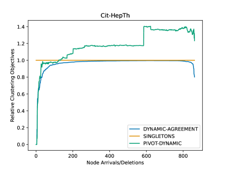
    Figure 2: Correlation clustering objective relative to singletons

    

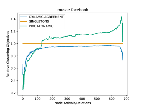
    Figure 3: Correlation clustering objective relative to singletons

    

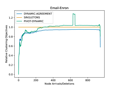
    Figure 4: Correlation clustering objective relative to singletons

References

Agrawal et al. ((2009))
R. Agrawal, A. Halverson, K. Kenthapadi, N. Mishra, and P. Tsaparas.
Generating labels from clicks.
In Proceedings of the 2nd ACM International Conference on Web
Search and Data Mining, pages 172–181, 2009.
Ailon et al. ((2008))
N. Ailon, M. Charikar, and A. Newman.
Aggregating inconsistent information: Ranking and clustering.
Journal of the ACM (JACM), 55(5), 2008.
Arasu et al. ((2009))
A. Arasu, C. Ré, and D. Suciu.
Large-scale deduplication with constraints using dedupalog.
In Proceedings of the 25th International Conference on Data
Engineering, pages 952–963, 2009.
Assadi and Wang ((2022))
S. Assadi and C. Wang.
Sublinear time and space algorithms for correlation clustering via
sparse-dense decompositions.
In Proceedings of the 13th Innovations in Theoretical Computer
Science Conference (ITCS), pages 10:1–10:20, 2022.
Bansal et al. ((2004))
N. Bansal, A. Blum, and S. Chawla.
Correlation clustering.
Machine learning, 56(1):89–113, 2004.
Bateni et al. ((2023))
M. Bateni, H. Esfandiari, H. Fichtenberger, M. Henzinger, R. Jayaram,
V. Mirrokni, and A. Wiese.
Optimal fully dynamic k-center clustering for adaptive and oblivious
adversaries.
In Proceedings of the 2023 Annual ACM-SIAM Symposium on
Discrete Algorithms (SODA), pages 2677–2727. SIAM, 2023.
Behnezhad et al. ((2019))
S. Behnezhad, M. Derakhshan, M. Hajiaghayi, C. Stein, and M. Sudan.
Fully dynamic maximal independent set with polylogarithmic update
time.
In D. Zuckerman, editor, 60th IEEE Annual Symposium on
Foundations of Computer Science, FOCS 2019, Baltimore, Maryland, USA,
November 9-12, 2019, pages 382–405. IEEE Computer Society, 2019.
doi: 10.1109/FOCS.2019.00032.
URL https://doi.org/10.1109/FOCS.2019.00032.
Behnezhad et al. ((2022))
S. Behnezhad, M. Charikar, W. Ma, and L. Tan.
Almost 3-approximate correlation clustering in constant rounds.
In 63rd IEEE Annual Symposium on Foundations of Computer
Science, FOCS 2022, Denver, CO, USA, October 31 - November 3, 2022, pages
720–731. IEEE, 2022.
doi: 10.1109/FOCS54457.2022.00074.
URL https://doi.org/10.1109/FOCS54457.2022.00074.
Behnezhad et al. ((2023a))
S. Behnezhad, M. Charikar, W. Ma, and L. Tan.
Single-pass streaming algorithms for correlation clustering.
In N. Bansal and V. Nagarajan, editors, Proceedings of the 2023
ACM-SIAM Symposium on Discrete Algorithms, SODA 2023, Florence, Italy,
January 22-25, 2023, pages 819–849. SIAM, 2023a.
doi: 10.1137/1.9781611977554.ch33.
URL https://doi.org/10.1137/1.9781611977554.ch33.
Behnezhad et al. ((2023b))
S. Behnezhad, M. Charikar, W. Ma, and L. Tan.
Single-pass streaming algorithms for correlation clustering.
In Proceedings of the 34th Annual ACM-SIAM Symposium on
Discrete Algorithms (SODA), pages 819–849, 2023b.
Bonchi et al. ((2013))
F. Bonchi, A. Gionis, and A. Ukkonen.
Overlapping correlation clustering.
Knowledge and information systems, 35(1):1–32, 2013.
Cao et al. ((2024))
N. Cao, V. Cohen-Addad, E. Lee, S. Li, A. Newman, and L. Vogl.
Understanding the cluster linear program for correlation clustering.
In B. Mohar, I. Shinkar, and R. O’Donnell, editors, Proceedings
of the 56th Annual ACM Symposium on Theory of Computing, STOC 2024,
Vancouver, BC, Canada, June 24-28, 2024, pages 1605–1616. ACM, 2024.
doi: 10.1145/3618260.3649749.
URL https://doi.org/10.1145/3618260.3649749.
Chakrabarti et al. ((2008))
D. Chakrabarti, R. Kumar, and K. Punera.
A graph-theoretic approach to webpage segmentation.
In Proceedings of the 17th International World Wide Web
Conference (WWW), pages 377–386, 2008.
Chawla et al. ((2015))
S. Chawla, K. Makarychev, T. Schramm, and G. Yaroslavtsev.
Near optimal lp rounding algorithm for correlation clustering on
complete and complete k-partite graphs.
In Proceedings of the 47th Annual ACM Symposium on Theory of
Computing (STOC), pages 219–228, 2015.
Chen et al. ((2012))
Y. Chen, S. Sanghavi, and H. Xu.
Clustering sparse graphs.
In Proceedings of the 25th Annual Conference on Neural
Information Processing Systems (NeurIPS), pages 2204–2212, 2012.
Cohen-Addad et al. ((2019))
V. Cohen-Addad, N. Hjuler, N. Parotsidis, D. Saulpic, and C. Schwiegelshohn.
Fully dynamic consistent facility location.
In Proceedings of the 33rd Annual Conference on Neural
Information Processing Systems (NeurIPS), 2019.
Cohen-Addad et al. ((2021))
V. Cohen-Addad, S. Lattanzi, S. Mitrovic, A. Norouzi-Fard, N. Parotsidis,
and J. Tarnawski.
Correlation clustering in constant many parallel rounds.
In Proceedings of the 38th International Conference on Machine
Learning (ICML), volume 139, pages 2069–2078, 2021.
Cohen-Addad et al. ((2022a))
V. Cohen-Addad, S. Lattanzi, A. Maggiori, and N. Parotsidis.
Online and consistent correlation clustering.
In Proceedings of the 39th International Conference on Machine
Learning (ICML), pages 4157–4179, 2022a.
Cohen-Addad et al. ((2022b))
V. Cohen-Addad, E. Lee, and A. Newman.
Correlation clustering with sherali-adams.
In 63rd IEEE Annual Symposium on Foundations of Computer
Science, FOCS 2022, Denver, CO, USA, October 31 - November 3, 2022, pages
651–661. IEEE, 2022b.
doi: 10.1109/FOCS54457.2022.00068.
URL https://doi.org/10.1109/FOCS54457.2022.00068.
Cohen-Addad et al. ((2023))
V. Cohen-Addad, E. Lee, S. Li, and A. Newman.
Handling correlated rounding error via preclustering: A
1.73-approximation for correlation clustering.
In 64th IEEE Annual Symposium on Foundations of Computer
Science, FOCS 2023, Santa Cruz, CA, USA, November 6-9, 2023, pages
1082–1104. IEEE, 2023.
doi: 10.1109/FOCS57990.2023.00065.
URL https://doi.org/10.1109/FOCS57990.2023.00065.
Cohen-Addad et al. ((2024))
V. Cohen-Addad, D. R. Lolck, M. Pilipczuk, M. Thorup, S. Yan, and H. Zhang.
Combinatorial correlation clustering.
In B. Mohar, I. Shinkar, and R. O’Donnell, editors, Proceedings
of the 56th Annual ACM Symposium on Theory of Computing, STOC 2024,
Vancouver, BC, Canada, June 24-28, 2024, pages 1617–1628. ACM, 2024.
doi: 10.1145/3618260.3649712.
URL https://doi.org/10.1145/3618260.3649712.
Demaine et al. ((2006))
E. D. Demaine, D. Emanuel, A. Fiat, and N. Immorlica.
Correlation clustering in general weighted graphs.
Theoretical Computer Science, 361(2-3):172–187, 2006.
Dua and Graff ((2017))
D. Dua and C. Graff.
UCI machine learning repository, 2017.
URL http://archive.ics.uci.edu/ml.
Epasto et al. ((2015))
A. Epasto, S. Lattanzi, and M. Sozio.
Efficient densest subgraph computation in evolving graphs.
In Proceedings of the 24th international conference on world
wide web, pages 300–310, 2015.
Fichtenberger et al. ((2021))
H. Fichtenberger, S. Lattanzi, A. Norouzi-Fard, and O. Svensson.
Consistent k-clustering for general metrics.
In Proceedings of the 32nd Annual ACM-SIAM Symposium on
Discrete Algorithms (SODA), pages 2660–2678. SIAM, 2021.
Guo et al. ((2021))
X. Guo, J. Kulkarni, S. Li, and J. Xian.
Consistent k-median: Simpler, better and robust.
In Proceedings of the 24th International Conference on
Artificial Intelligence and Statistics, pages 1135–1143, 2021.
Jaghargh et al. ((2019))
M. R. K. Jaghargh, A. Krause, S. Lattanzi, and S. Vassilvtiskii.
Consistent online optimization: Convex and submodular.
In Proceedings of the 22nd International Conference on
Artificial Intelligence and Statistics, pages 2241–2250, 2019.
Kalashnikov et al. ((2008))
D. V. Kalashnikov, Z. Chen, S. Mehrotra, and R. Nuray-Turan.
Web people search via connection analysis.
IEEE Transactions on Knowledge and Data Engineering,
20(11):1550–1565, 2008.
Lattanzi and Vassilvitskii ((2017))
S. Lattanzi and S. Vassilvitskii.
Consistent k-clustering.
In Proceedings of the 34th International Conference on Machine
Learning (ICML), pages 1975–1984, 2017.
Lattanzi et al. ((2021))
S. Lattanzi, B. Moseley, S. Vassilvitskii, Y. Wang, and R. Zhou.
Robust online correlation clustering.
In Proceedings of the 34th Annual Conference on Neural
Information Processing Systems (NeurIPS), 2021.
Leskovec and Krevl ((2014))
J. Leskovec and A. Krevl.
SNAP Datasets: Stanford large network dataset collection.
http://snap.stanford.edu/data, 2014.
Rodriguez-Lujan et al. ((2014))
I. Rodriguez-Lujan, J. Fonollosa, A. Vergara, M. Homer, and R. Huerta.
On the calibration of sensor arrays for pattern recognition using the
minimal number of experiments.
Chemometrics and Intelligent Laboratory Systems, 130:123–134, 2014.
Vergara et al. ((2012))
A. Vergara, S. Vembu, T. Ayhan, M. A. Ryan, M. L. Homer, and R. Huerta.
Chemical gas sensor drift compensation using classifier ensembles.
Sensors and Actuators B: Chemical, 166:320–329,
2012.