AdaRevD: Adaptive Patch Exiting Reversible Decoder
Pushes the Limit of Image Deblurring

Abstract

Despite the recent progress in enhancing the efficacy of image deblurring, the limited decoding capability constrains the upper limit of State-Of-The-Art (SOTA) methods. This paper proposes a pioneering work, Adaptive Patch Exiting Reversible Decoder (AdaRevD), to explore their insufficient decoding capability. By inheriting the weights of the well-trained encoder, we refactor a reversible decoder which scales up the single-decoder training to multi-decoder training while remaining GPU memory-friendly. Meanwhile, we show that our reversible structure gradually disentangles high-level degradation degree and low-level blur pattern (residual of the blur image and its sharp counterpart) from compact degradation representation. Besides, due to the spatially-variant motion blur kernels, different blur patches have various deblurring difficulties. We further introduce a classifier to learn the degradation degree of image patches, enabling them to exit at different sub-decoders for speedup. Experiments show that our AdaRevD pushes the limit of image deblurring, e.g., achieving 34.60 dB in PSNR on GoPro dataset.

1 Introduction

As a sub-task of image restoration, image deblurring aims at removing degraded blur artifacts to recover clean images. Generally, two types of backbone networks, i.e., multi-stage and one-stage architectures, consisting of multiple encoders and decoders, have been proposed for the image deblurring task. Encoders are used to learn a compact degradation representation from a blur image and decoders decode the degradation representation to blur patterns. The compact degradation representation can be treated as a mid-level feature, equipped with high-level degradation degree information and low-level blur pattern. See Fig. 8 and Sec. 4.3.1 for detailed analysis.

Multi-stage architectures [25, 42, 4] (see Fig. 1 (a)) decompose the feature extraction process into multiple sub-networks. Recent research explorations for image restoration [43, 36, 5] have shown the ability of one-stage architecture (see Fig. 1 (b)). Instead of focusing on the overall design of the model, more attention is paid to the core components design of the one-stage architecture, such as Res-Block [12] and Transformer-Block [34]. In fact, several one-stage architectures have delicately designed heavyweight encoders. MSDI-Net [20] introduces an extra degradation representation encoder to enhance the image deblurring performance. In UFPNet [10], the kernel prior module is pre-trained to estimate the spatially variant blur kernel information, which is then integrated into the encoder. Although the encoder is delicately designed to learn robust degradation representation, the size of the whole network is limited to what the GPU can accommodate. Thus, these networks have to design lightweight decoders to decode blur patterns from the degradation representation. Insufficient decoding capability constrains the model’s upper limit.

The performance of existing image deblurring networks reaches saturation when training is completed, signifying the performance pinnacle of the current network. Even with more training iterations, the performance remains unchanged, or even leads to a decrease in performance, as shown in Fig. 1 (d). But, constrained by the lightweight decoders, the deblurring results may not be optimal. This makes us wonder: Is it possible to inherit the weights of the well-trained encoder and refactor the decoder with high capacity, enabling us to map the learned degradation representation to the blur pattern more effectively and push the limits of image deblurring?

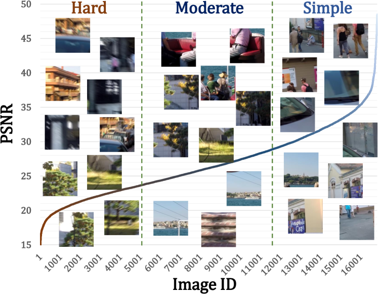
Figure 2: The ranked PSNR curve of the image patches from GoPro [25] train set and the visualization of the patches with various degradation degrees (e.g. hard, moderate and simple).

A straightforward solution is to refactor the original decoder with a heavyweight decoder, and retrain the network by only updating the decoder. Since the capability of the decoder is constrained by the GPU memory, a memory-saving learning paradigm is important, especially for large models. Besides, for a typical decoder, layers close to the encoder contain more high-level degradation information, while features close to the output are decoded blur patterns, indicating the pixel-level residual between blur and sharp images. Learning a direct mapping from a compact degradation representation to the pixel-level blur pattern like previous decoders may suffer from inferior performances during testing, since information unrelated to the target details may be gradually decoded and accumulated during the layer-by-layer propagation due to the UNet architecture.

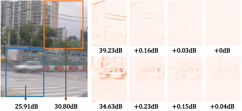
Figure 3: Visual comparison of the outputs from different sub-decoders. The first column is the difference between blur image and the first sub-decoder’s output. The rest of the columns are the residual between the current sub-decoder and the former one.

To solve the problems and push the limit of image deblurring model, we propose an Adaptive Patch Exiting Reversible Decoder (AdaRevD), as shown in Fig. 1(c). Concretely, our decoder is composed of $K$ sub-decoders, trained in a reversible manner [3], each of which takes the degradation representation as input and generates a sharp prediction. A sub-decoder consists of multi-level features, from high-level semantics to low-level blur patterns. This design enables a large model capacity while consuming only limited GPU memory. It progressively separates low-level and high-level information by disentangling features. It is the first attempt to train a memory-friendly decoder in a backward feature propagation manner without loss of information in the field of high-resolution image deblurring.

Additionally, as shown in Fig. 2 and Fig. 3, given the varying degrees of blur in image patches, the difficulty of restoring each patch varies. With gradually stacking more sub-decoders, the restoration performances of different patches may reach bottlenecks. Due to the obstacles brought by the deblurring network’s multi-scale feature property, no prior work attempts to design an exiting strategy for image deblurring. Thanks to our sub-decoder structures, we design an adaptive patch exiting strategy effortlessly. We employ a classifier to predict the degradation degree of each blur patch, allowing a patch to exit at a specific sub-decoder to achieve speedup.

The main contributions can be summarized as follows:

• We propose a first work to push the limit of State-Of-The-Art (SOTA) image deblurring networks by exploring their insufficient decoding capability.

• We propose a reversible deblurring decoder with a substantial capacity while remaining GPU memory-friendly. Meanwhile, it gradually disentangles high-level degradation degree and low-level task-related features, learning blur patterns while maintaining the overall semantics.

• We propose a simple classifier to get the degradation degree of the input image, enabling the patches to exit at various decoders for speedup.

• Extensive experiments show that our proposed AdaRevD can push the limit of image deblurring. It achieves SOTA results on image deblurring task, e.g., 34.60 dB in PSNR for GoPro dataset. The PSNR (dB) vs. GPU-memory (G) compared with others is shown in Fig. 1 (e).

2 Related Works

2.1 Deblurring Methods

Recently, many methods [25, 31, 18, 21, 44, 42, 7, 24, 33, 5, 37, 43, 10, 15] apply end-to-end trained deep neural network for image deblurring. In order to achieve better performance, most improvements are made around the model structure or the specific component. For the structure, many studies such as DeepDeblur [25], DMPHN [44] and MPRNet [42] prefer to use multi-stage architecture, which learns degradation pattern progressively. The diffusion-based work [37] trains a stochastic sampler that refines the output of a deterministic predictor. Per contra, the design of specific block with UNet shows its capacity of deblurring. NAFNet [5] applies LayerNorm (LN) [1] to stabilize the training process with a high initial learning rate. Uformer [36] and Stripformer [32] apply Local Self-Attention (SA) to capture long-range dependencies with low complexity. Restormer [43] models global context by Global Channel SA. DeepRFT [24] proposes Res-FFT-ReLU-Block for frequency selection. MRLPFNet [9] constructs Residual Low-Pass Filter Module based on DeepRFT [24] and Restormer [43]. However, few methods consider the varying levels of image degradation.

2.2 Reversible Architectures

In the process of gradient backpropagation, a lot of resources are used to store intermediate features. As the networks become deeper and wider for SOTA performance, GPU memory has been a bottleneck limiting the further development of the model. To solve this bottleneck, Reversible Residual Block (RevBlock) [11] lets each block’s activations be reestablished from the following ones. i-RevNet [13] builds a fully inverted network by providing an explicit inverse. Rev-ViT [23] extends reversible CNN block to reversible Transformer block, which promotes saving GPU memory and allows training ViT model with higher batch size. RevBiFPN [6] builds a fully reversible bidirectional feature pyramid network by BiFPN [30]. RevCol [3] proposes a reversible column-based foundation model design paradigm. In accordance with this paradigm, our AdaRevD is the inaugural endeavor to incorporate reversible columns as sub-decoders for image deblurring. This approach maintains a consistent consumption of GPU memory during training, akin to a single sub-decoder. Furthermore, the utilization of multiple sub-decoders facilitates the exit of the network’s forward propagation through the pertinent sub-decoder.

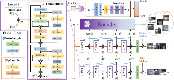
Figure 4: Architecture of AdaRevD. AdaRevD consists of three parts: a pre-trained encoder, several sub-decoders and a classifier. To push the limit of image deblurring networks, and map the learned degradation representation to the blur pattern more effectively, the pre-trained encoder is fixed during training. Each sub-decoder is composed of four Level modules, including a Fuseblock and a FourierBlock. SCA means Simple Channel Attention proposed in NAFNet [5]. The classifier predicts the degradation degree of each image patch, which allows the network to exit in the appropriate sub-decoder.

2.3 Adaptive Inference

Since the kernels are always spatially-variant for the blur image, different patches receive various degrees of degradation. Facing the deployment of neural networks under different conditions, many methods [41, 40, 39, 14, 38, 2, 22, 16, 35] are proposed to permit instant and adaptive accuracy-efficiency trade-offs at runtime. Slimmable networks [41] enable a single network executable at different widths which can instantly adjust the width in runtime. For image super-resolution, different image regions usually have various restoration difficulties [35]. AdaDSR [22] introduces a lightweight adapter module to predict the network depth map, which facilitates efficient adaptive inference with sparse convolution. ClassSR [16] classifies the repair difficulty of patches into three types: easy, medium, and difficult. Different types are restored by various networks. APE-SR [35] exits early in the intermediate ResBlocks by using a simple regressor to estimate the incremental prediction. Unlike the image super-resolution models which apply a sequence of ResBlocks [12] without down-sample and up-sample as the main body, deblurring models always tend to use UNet [28] model. However, The structure of UNet model is not conducive to exit in different stages. Thus, it is difficult to apply these adaptive patterns to deblurring model directly. In AdaRevD, we construct a multi-decoder architecture with a degradation degree classifier, enabling the possibility to exit in different sub-decoders.

3 Method

3.1 Main Backbone

Recently, deep learning based deblurring methods always employ a network composed of four parts: head, encoder, decoder and tail, which directly map a blur image to its paired sharp image. This architectural design has gained mainstream prominence in recent years [5]. The head part usually applies a $3\times 3$ convolutional layer, whose parameters are denoted as $\mathbf{\Theta}_{head}$ to extract shallow features $\mathbf{h}$ from blur image $\mathbf{B}$:

$$\mathbf{h}=\mathcal{H}(\mathbf{B},\mathbf{\Theta}_{head}).\vspace{-0.5em}$$ (1)

Then, the encoder, parameterized by $\mathbf{\Theta}_{enc}$, takes $\mathbf{h}$ as the input and generates $N$ hidden features $\mathbf{e}_{1}$, $\mathbf{e}_{2}$, …, $\mathbf{e}_{N}$:

$$\mathbf{e}_{1},\mathbf{e}_{2},...,\mathbf{e}_{N}=\mathcal{E}(\mathbf{h},\mathbf{\Theta}_{enc}).\vspace{-0.5em}$$ (2)

After that, the decoder, parameterized by $\mathbf{\Theta}_{dec}$, decodes the hidden features as the blur pattern feature $\mathbf{d}_{1}$:

$$\mathbf{d}_{1}=\mathcal{D}(\mathbf{e}_{1},\mathbf{e}_{2},...,\mathbf{e}_{N},\mathbf{\Theta}_{dec}).\vspace{-0.5em}$$ (3)

At last, the tail part, parameterized by $\mathbf{\Theta}_{tail}$, takes the degradation feature to obtain the blur pattern $\mathbf{t}$ with a $3\times 3$ convolutional layer and obtain the restored sharp image $\hat{\mathbf{S}}$:

$$\mathbf{t}=\mathcal{T}(\mathbf{d}_{1},\mathbf{\Theta}_{tail})$$ (4)

$$\hat{\mathbf{S}}={\mathbf{B}}+\mathbf{t}.\vspace{-0.5em}$$ (5)

In our AdaRevD, we construct a multi-decoder structure. The intermediate feature from Level $i$ of $j$th sub-decoder is denoted as $\mathbf{d}_{i}^{j}$. Thus, Eq. 3 is rewritten as:

$$\mathbf{d}_{1}^{1},...,\mathbf{d}_{N-1}^{1} =\mathcal{D}^{1}(\mathbf{e}_{1},...,\mathbf{e}_{N},\mathbf{\Theta}_{dec}^{1}),$$ (6)

$$\mathbf{d}_{1}^{k},...,\mathbf{d}_{N-1}^{k} =\mathcal{D}^{1}(\mathbf{d}_{1}^{k-1},...,\mathbf{d}_{N-1}^{k-1},\mathbf{e}_{N},\mathbf{\Theta}_{dec}^{k}).\vspace{-0.5em}$$ (7)

Finally, the restored sharp image from $j$th decoder is:

$$\hat{\mathbf{S}}^{j}=\mathbf{B}+\mathcal{T}^{j}(\mathbf{d}_{{1}}^{j},\mathbf{\Theta}_{tail}^{j}).\vspace{-0.5em}$$ (8)

The overview of AdaRevD is shown in Fig. 4. Different from RevCol [3] , which separates the encoder into multiple reversible sub-encoders, AdaRevD builds a reversible model which contains multiple reversible sub-decoders. For practical speedup, we design an adaptive patch-exiting method on top of the reversible structures to determine whether to early exit in various sub-decoders by a classifier.

There are two training phases in AdaRevD: decoder training and classifier training. In decoder training, AdaRevD optimizes the decoder based on the well trained encoder from UFPNet [10] and keeps the encoder frozen during training for lower memory consumption. In the classifier training phase, only the classifier will be optimized. Thanks to the reversible architecture, AdaRevD can enhance the size of a single-stage model, thereby equipping it with a larger capacity, all while maintaining low memory requirements. Thanks to our adaptive classifier, AdaRevD enables the patch to exit at the optimal layer. For sub-decoders, we propose a FourierBlock for large-scale sensing capability purposes. From Level-1 to Level-4, the number of blocks are $[1,1,1,1]$ (each sub-decoder).

3.2 Reversible Decoder

Forward and Inverse Structure

RevCol [3] builds a reversible column architecture composed of multiple sub-networks (columns) in the encoder for classification-related tasks. But, image deblurring models [10, 5] are usually designed with very heavy encoders. Thus, fewer benefits can be gained from reversible architectures. Instead, we propose reversible decoders which take reversible columns as sub-decoders to save the GPU memory consumption during training. It is worth noting that the reversible decoder facilitates the utilization of early exit when representations are presented in a hierarchical multi-scale manner. Formally, the forward and inverse computations are:

$$\small\text{Forward: }\mathbf{d}_{i}^{j}=\begin{cases}\mathcal{L}_{i}^{j}(\mathbf{d}_{i+1}^{j},\mathbf{d}_{i-1}^{j-1})+\alpha\mathbf{d}_{i}^{j-1}~{}~{}~{}~{}~{}&i>1\\ \mathcal{L}_{i}^{j}(\mathbf{d}_{i+1}^{j})+\alpha\mathbf{d}_{i}^{j-1}~{}~{}~{}~{}~{}&i=1\end{cases}\vspace{-0.5em}$$ (9)

$$\small\text{Inverse: }\mathbf{d}_{i}^{j-1}=\begin{cases}\alpha^{-1}(\mathbf{d}_{i}^{j}-\mathcal{L}_{i}^{j}(\mathbf{d}_{i+1}^{j},\mathbf{d}_{i-1}^{j-1}))~{}&i>1\\ \alpha^{-1}(\mathbf{d}_{i}^{j}-\mathcal{L}_{i}^{j}(\mathbf{d}_{i+1}^{j}))~{}&i=1\end{cases}\vspace{-0.5em}$$ (10)

where $\mathcal{L}_{i}^{j}$ is the $i$th Level module of $j$th decoder , $\mathbf{d}_{i}^{j}$ is the output feature of the $i$th Level in the $j$th decoder, $\alpha$ is the learnable scaling parameter.

Level Module

The Level modules in reversible decoders are composed of two blocks: FuseBlock and FourierBlock. Because reversible architecture can help us save the training memory, heavier modules can be used to replace the NAFBlock [5] for further improvement of deblurring. In AdaRevD, we apply a Fuseblock to fuse the feature maps from the current and previous sub-decoder and a FourierBlock [24] to decode better blur pattern.

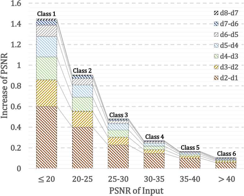
Figure 5: The increment for degraded patches belonging to each degradation degree class in different sub-decoders. The patches are generated from GoPro [25] train set. d$(i)$-d$(i-1)$ means the average increment PSNR for the patches in the $i$th sub-decoder.

3.3 Adaptive Classifier

In order to establish a multi-exit deblur model, we design a multi-decoder structure which predicts sharp images in each sub-decoder. Generally, the performance of the model usually increases when the model goes deeper. However, the blur kernels are always spatially-variant, which means the recoverability of image patches varies. Fig. 3 and Fig. 5 indicate that the incremental capacity of each sub-decoder varies with different degraded patches. There is no need to cost overmany sub-decoders for the patches whose PSNRs are already high, e.g., higher than 40 dB. For GoPro [25] dataset, we group the patches to 6 degradation degrees ($\tilde{c}$) via the PSNR between the blur patch and the sharp patch: ($\leq$ 20 dB, $\tilde{c}=1$), ($\leq$ 25 dB, $\tilde{c}=2$), ($\leq$ 30 dB, $\tilde{c}=3$), ($\leq$ 35 dB, $\tilde{c}=4$), ($\leq$ 40 dB, $\tilde{c}=5$) and ($>$ 40 dB, $\tilde{c}=6$). Then, an additional classifier is introduced to predict the degradation degree of the blur patch:

$$\hat{{c}} =\mathtt{Classifier}(\mathbf{e}_{4}).$$ (11)

The classifier takes $\mathbf{e}_{4}$ as the input and predicts the degradation degree classification $\hat{{c}}$ of the input patch. As indicated in Fig. 4, the classifier contains a DownSample layer, an NAFBlock, a LayerNorm layer and an MLP (GAP-Linear-GELU-Linear) block. $\mathtt{GAP}$ means global average pooling.

To avoid consuming computing resources on simple patches, we define the early-exit signal ${E}_{c}$, indicating which sub-decoder to exit when processing a patch belonging to the $c$th class. ${E}_{c}$ is defined as:

$$E_{c}=\left\{\begin{array}[]{cl}j-1,{}{}{}&\text{if}~{}~{}~{}{\exists}~{}\mathbf{O}_{c}^{j}<\tau,\\ J,{}{}{}&\text{otherwise},\end{array}\right.\vspace{-0.5em}$$ (12)

where $J$ means the total sub-decoder number, $\tau$ is a pre-defined threshold, and $\mathbf{O}_{c}^{j}$ is collected during the training process, calculated as:

$$\mathbf{O}_{c}^{j}=\frac{1}{|\Omega_{c}|}\sum_{\mathbf{P}\in\Omega_{c}}\mathtt{PSNR}(\hat{\mathbf{P}}^{j},\mathbf{P})-\mathtt{PSNR}(\hat{\mathbf{P}}^{j-1},\mathbf{P}),\vspace{-0.5em}$$ (13)

where $\mathbf{P}$ is a sharp patch and $\Omega_{c}$ means the set of sharp patches whose corresponding blur patches belong to the $c$th class. $|\Omega_{c}|$ is the cardinality of $\Omega_{c}$. $\hat{\mathbf{P}}^{j}$ means the prediction from the $j$th sub-decoder. With the incremental prediction $\mathbf{O}_{c}^{j}$ and the degradation degree classification $\hat{\mathbf{C}}$ of the input patch, AdaRevD is able to let the patch exit in the $(j-1)$th sub-decoder when $\mathbf{O}_{c}^{j}$ is smaller than the threshold $\tau$.

(a) Blur

(b) MPRNet [42]

(c) Restormer [43]

(d) DeepRFT+[24]

(e) NAFNet64 [5]

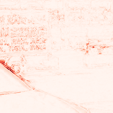
(f) UFPNet[10]

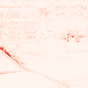
(g) Ours

(h) Sharp

Figure 6: Examples on the GoPro test dataset. The first row shows blur image, predicted images of different methods, and ground-truth sharp image. The second row shows the residual of the blur image / predicted sharp images and the ground-truth sharp image.

3.4 Loss Function

For decoder training phase, the loss is defined as:

$$\ell_{m}=\ell_{1}+0.01\ell_{fr}\vspace{-0.5em}$$ (14)

where $\ell_{1}=\frac{1}{N}\sum_{j=1}^{K}||{\hat{\mathbf{S}}^{j}}-{\mathbf{S}}||_{1}$ and $\ell_{fr}=\frac{1}{K}\sum_{j=1}^{K}||\mathcal{F}({\hat{\mathbf{S}}^{j}})-\mathcal{F}({\mathbf{S}})||_{1}$. $\mathcal{F}(\cdot)$ represents 2D Fast Fourier Transform. The loss is uniformly applied to each sub-decoder with the same weight.

For classifier-training phase, Cross Entropy Loss is used to measure the difference between $\hat{{c}}$ and ground-truth degradation degree classification $\tilde{c}$:

$$\ell_{c}=\mathtt{CrossEntropy}(\tilde{c},\hat{{c}})\vspace{-0.5em}$$ (15)

4 Experiment

4.1 Experimental Setup

Dataset

We evaluate our method on the four datasets: GoPro [25] / HIDE [29] / RealBlur-R / RealBlur-J [27]. GoPro dataset is also used for the experiments in Sec. 4.3. More details will be shown in the supplementary material.

Model Configuration

We build 3 reversible decoder models based on the trained encoder from NAFNet [5] and UFPNet (default) [10]: RevD-S (2 sub-decoders), RevD-B (4 sub-decoders) and RevD-L (8 sub-decoders). Because of the various distributions of different datasets, the class number varies. The patches from GoPro [25] and RealBlur-J [27] are divided into 6 classes. Besides, there are 8 classes for RealBlur-R [27]. With the degradation degree classifier, AdaRevD-B and AdaRevD-L apply adaptive patch exiting based on various incremental predictions of different sub-decoders from the train set. The threshold $\tau$ is configured to 0.05 for the early-exit signal ${E}_{c}$. More details will be shown in the supplementary material.

Table 1: Comparison on GoPro [25], HIDE [29] and RealBlur [27] datasets for setting $\mathcal{A}$.

	GoPro	HIDE	RealBlur-R	RealBlur-J
Method	PSNR SSIM	PSNR SSIM	PSNR SSIM	PSNR SSIM
DeepDeblur [25]	29.08 0.914	25.73 0.874	32.51 0.841	27.87 0.827
SRN [31]	30.26 0.934	28.36 0.915	35.66 0.947	28.56 0.867
DMPHN [44]	31.20 0.940	29.09 0.924	35.70 0.948	28.42 0.860
DBGAN [45]	31.10 0.942	28.94 0.915	33.78 0.909	24.93 0.745
MT-RNN [26]	31.15 0.945	29.15 0.918	35.79 0.951	28.44 0.862
MPRNet [42]	32.66 0.959	30.96 0.939	35.99 0.952	28.70 0.873
HINet [4]	32.71 0.959	30.32 0.932	-	-
MIMO-UNet+ [7]	32.45 0.957	29.99 0.930	35.54 0.947	27.63 0.837
Whang [37]	33.23 0.963	-	-	-
Uformer [36]	33.06 0.967	30.90 0.953	36.19 0.956	29.09 0.886
NAFNet64 [5]	33.69 0.967	31.32 0.943	35.84 0.952	27.94 0.854
Stripformer [32]	33.08 0.962	31.03 0.940	-	-
Restormer [43]	32.92 0.961	31.22 0.942	36.19 0.957	28.96 0.879
DeepRFT+ [24]	33.52 0.965	31.66 0.946	36.11 0.955	28.90 0.881
FFTformer [15]	34.21 0.968	31.62 0.946	-	-
UFPNet [10]	34.06 0.968	31.74 0.947	36.25 0.953	29.87 0.884
MRLPFNet [9]	34.01 0.968	31.63 0.947	-	-
RevD-S(UFPNet)	34.35 0.970	32.08 0.950	36.56 0.957	30.09 0.892
RevD-B(NAFNet)	34.10 0.969	31.86 0.948	36.04 0.952	28.46 0.863
RevD-B(UFPNet)	34.51 0.971	32.27 0.952	36.58 0.957	30.12 0.893
AdaRevD-B	34.50 0.971	32.26 0.952	36.56 0.957	30.12 0.894
RevD-L(NAFNet)	34.18 0.970	31.93 0.948	36.03 0.952	28.46 0.863
RevD-L(UFPNet)	34.64 0.972	32.37 0.953	36.60 0.958	30.14 0.895
AdaRevD-L	34.60 0.972	32.35 0.953	36.53 0.957	30.12 0.894

Table 2: Comparison on RealBlur [27] for setting $\mathcal{B}$.

	RealBlur-R	RealBlur-J	Average	Memory
Method	PSNR SSIM	PSNR SSIM	PSNR SSIM	(MB)
DeblurGAN-v2 [19]	36.44 0.935	29.69 0.870	33.07 0.903	-
SRN [31]	38.65 0.965	31.38 0.909	35.02 0.937	-
MPRNet [42]	39.31 0.972	31.76 0.922	35.54 0.947	6,294
MAXIM [33]	39.45 0.962	32.84 0.935	36.15 0.949	-
Stripformer [32]	39.84 0.974	32.48 0.929	36.16 0.952	3,449
DeepRFT+ [24]	40.01 0.973	32.63 0.933	36.32 0.953	3,569
FFTformer [15]	40.11 0.975	32.62 0.933	36.37 0.954	19,800
UFPNet [10]	40.61 0.974	33.35 0.934	36.98 0.954	8,164
MRLPFNet [9]	40.92 0.975	33.19 0.936	37.06 0.956	-
RevD-B	41.10 0.978	33.84 0.943	37.47 0.961	3,386
AdaRevD-B	41.09 0.978	33.84 0.943	37.47 0.961	-
RevD-L	41.22 0.979	33.99 0.944	37.61 0.962	5,087
AdaRevD-L	41.19 0.979	33.96 0.944	37.58 0.962	-

Implementation Details and Evaluation Metric

We adopt the training strategy from NAFNet [5] unless otherwise specified. I.e., the network training hyperparameters (and the default values) are data augmentation (horizontal and vertical flips), optimizer Adam ($\beta_{1}=0.9$, $\beta_{2}=0.9$, weight decay 1$\times$10^-3), initial learning rate (1$\times$10^-3). The learning rate is steadily decreased to 1$\times$10^-7. RevD is trained with patch size 256$\times$256 and batch size 16 for 200K iterations with ema decay 0.999. For AdaRevD, an additional classifier is trained based on the pre-trained encoder with patch size 384$\times$384 and batch size 16 for 10K iterations. Due to the spatially-variant kernel and statistics distribution shifts between training and testing [8], we utilize a step of 352 sliding window strategy with the window size of 384$\times$384, and an overlap size of 32 for testing.

Performances in terms of PSNR and SSIM over all testing sets are calculated using official algorithms. Besides, GPU memory is calculated by training a single patch size 256$\times$256 image with NVIDIA GeForce RTX 3090 GPU.

4.2 Main Results

Setting $\mathcal{A.}$

Our models are trained on 2,103 image pairs from GoPro [25], and compared with other SOTA methods through the test set of GoPro [25] , HIDE [29] and RealBlur [27]. As shown in Table 1, AdaRevD outperforms the other models in both PSNR and SSIM on the GoPro and HIDE test set. Besides, AdaRevD-B obtains robust results on other datasets. For example, AdaRevD-B achieves 36.56 / 30.12 dB on RealBlur-R / J test set, 0.31 / 0.25 dB higher than UFPNet [10]. Figure 6 shows the visual comparison on GoPro test set. Our approach extends the capabilities of the well-trained encoder by enhancing its capacity. In comparison to other SOTA methods, ours effectively minimizes a greater amount of the blur pattern.

Setting $\mathcal{B.}$

Our models are trained and tested on RealBlur-J / RealBlur-R  [27] respectively. As seen in Table 2, AdaRevD-B / L achieves 33.84 / 33.96 dB on RealBlur-J test set, 0.49 / 0.61 dB higher than UFPNet [10]. Figure 7 shows the visual comparison on RealBlur-J test set. In comparison with alternative approaches, our method excels in producing cleaner image restorations. Specifically, when applied to RealBlur-R, AdaRevD-L achieves a superior outcome (41.19 dB) compared to UFPNet (40.61 dB).

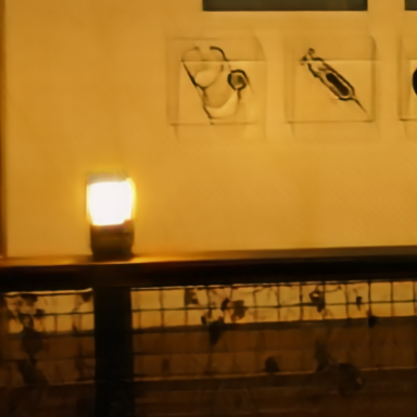
(a) DeepRFT+ [24]

(b) Stripformer [32]

(c) UFPNet [10]

(d) Ours

Figure 7: Examples on the RealBlur-J test dataset.

4.3 Analysis and Discussions

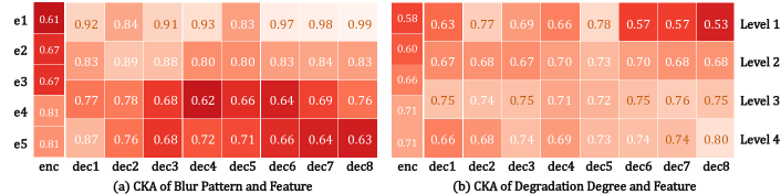
Figure 8: CKA similarities [17] of features and blur pattern / degradation degree for different levels and decoders. The blur pattern is obtained by subtracting the blur image from the ground-truth sharp image. The degradation degree comes from the feature after the NAFBlock in the classifier.

4.3.1 Effect of Reversible Image Deblurring

Memory Consumption

In AdaRevD, we propose to enhance the size of a single-stage model with the reversible sub-decoders. As indicated in Table 3, the cost of training memory is more friendly for reversible architecture when the size of the model is increasing. The memory consumption of a non-reversible architecture increases at a much faster rate than that of a reversible architecture as the number of sub-decoders rises.

FourierBlock

As shown in Table 4, compared with the original NAFBlock [5], FourierConv (RFFT2d-1$\times$1Conv-GELU-1$\times$1Conv-IRFFT2d) can significantly boost the model’s performance from 34.15 dB to 34.51 dB.

Retrain on SOTA Methods

Since our AdaRevD retrains on the encoder of SOTA methods, we also train original SOTA methods with more iterations to see what the results are. As shown in Table 5, if we allow the well-trained model to undergo additional iterations using the same training strategy, the improvement is marginal for NAFNet [5]. We also perform experiments to investigate the impact of freezing the encoder, and the results are reported in the Table 5. For UFPNet [10], keeping both encoder and decoder training for more iterations would even cause a decrease from 34.09 dB (freezing encoder) to 33.71 dB. To conserve additional GPU memory, AdaRevD investigates the construction of a multi-decoder architecture by leveraging a frozen encoder from from other SOTA methods.

Table 3: Performance of different sub-decoders. Dec-Idx is the sub-decoder number. Non-Rev means reversible mode is not used.

	Dec-Idx	1	2	3	4	5	6	7	8
RevD-S	PSNR	34.142	34.348	-	-	-	-	-	-
RevD-B	(dB)	34.074	34.313	34.459	34.515	-	-	-	-
RevD-L		34.020	34.287	34.376	34.481	34.577	34.620	34.635	34.640
Reversible	Memory	1,980	2,537	2,960	3,386	3,810	4,233	4,660	5,087
Non-Rev	(MB)	1,980	3,260	4,548	5,834	7,111	8,398	9,676	10,960

Table 4: Ablation studies. Num-Dec is sub-decoder’s number. $N$* means using a decoder with $N$ blocks for each level.

FuseBlock	FourierBlock		Num-Dec	Memory	PSNR
	NAFBlock	Fourier		(MB)	(dB)
$\times$	✓	$\times$	4	1,864	34.03
✓	✓	$\times$	4	1,974	34.15
$\times$	✓	✓	4	3,258	34.24
✓	✓	✓	2*	3,124	34.15
✓	✓	✓	4	3,386	34.51
✓	✓	✓	4*	5,387	34.49
✓	✓	✓	8	5,087	34.64

Disentanglement of Degradation Representation and Blur Pattern

We use Centered Kernel Alignment (CKA) similarity metric [17] to measure the similarity between learned features in RevD-L and blur pattern (residual between the blur image and its sharp counterpart), as well as the similarity between learned features and degradation degree (output feature of NAFBlock in Classifier), shown as the $2$nd $\sim$ $9$th columns in Fig. 8(a) and Fig. 8(b). Besides, we also compute the similarity between encoder features and the blur pattern / degradation degree, shown in the first columns. The encoder features (enc, $\mathbf{e}_{1}\sim\mathbf{e}_{5}$) gradually learn mid-level degradation representation which is mixed with the information of low-level blur pattern and high-level degradation degree.

For features of Level 1$\sim$Level 4 in 8 sub-decoders, we observe two intriguing phenomenons: (1) One sub-decoder (dec1) cannot decode the accurate blur pattern from degradation representations (see the $2$nd column in Fig. 8(a)). This may be due to the reason that encoder features in an UNet architecture inevitably bring information unrelated to the target details to decoder features via operations such as skip connections. Details related to the input blur image itself are likely to be superimposed on the decoder features. Thus, the target blur pattern (residual between the blur and sharp images) cannot be decoded precisely. (2) reversible sub-decoders enable the ability to gradually disentangle low-level blur pattern and high-level degradation degree (see the $2$nd to the last column in Fig. 8). If we observe the $2$nd to the last column in Fig. 8 row-by-row, it is obvious that more accurate low-level blur patterns are learned from Level modules connected to the output (e.g., Level 1 in Fig. 8(a)), and more high-level degradation degree knowledge is gathered from Level modules connected to the encoder (e.g., Level 4 in Fig. 8(b)).

Table 5: Comparison for continued training on SOTA methods. For UFPNet, since we freeze the kernel prior model, the training memory reduces from 8,164 MB (in Table 2) to 4,311 MB.

Model	NAFNet		UFPNet
Encoder trainable	✓	$\times$	✓	$\times$
Memory (MB)	3,394	1,160	4,311	1,617
PSNR (dB)	33.75	33.70	33.71	34.09

Table 6: Ablation for classifier. Reg and Cls means regressor and classifier respectively. Reg($\mathbf{d}_{4}^{k-1}$) indicates that the regressor takes $\mathbf{d}_{4}^{k-1}$ as input and output the incremental prediction for the $k$th sub-decoder. $\tau$ is the threshold for the regressor and the early-exit signal ($E_{c}$ in Eq. 12). The numbers for ${E}_{1}\sim{E}_{6}$ mean the specific sub-decoder to exit for a patch. Acc is the accuracy of the classifier. L1 is the L1 distance between the regressor’s output and the real increment of each sub-decoder. D-Rate means the utilization rate of the sub-decoders.

	$\tau$	${E}_{1}$	${E}_{2}$	${E}_{3}$	${E}_{4}$	${E}_{5}$	${E}_{6}$	Acc / L1	PSNR	D-Rate
RevD-B	-	4	4	4	4	4	4	-	34.515	100.0%
	-	3	3	3	3	3	3	-	34.459	75.0%
Reg($\mathbf{d}_{4}^{k-1}$)	0.05	-	-	-	-	-	-	0.071	34.497	82.5%
	0.10	-	-	-	-	-	-		34.457	65.9%
Cls($\mathbf{e}_{5}$)	0.05	4	4	3	2	1	1	84.43%	34.502	85.8%
	0.10	4	3	2	2	1	1		34.437	62.1%
Cls($\mathbf{e}_{4}$)	0.05	4	4	3	2	1	1	89.84%	34.501	84.3%
	0.10	4	3	2	2	1	1		34.436	60.6%

4.3.2 Effect of Adaptive Patch Exiting

Patch-exiting has been proposed in super-resolution tasks, whose modules usually learn features with the same scale [35]. Thus, in image deblurring, no prior work has been attempted to design a patch-exiting method. Different from ClassSR [16] and APE-SR [35], AdaRevD builds an adaptive patch exiting model based on multiple sub-decoders and a simple classifier. ClassSR [16] has to train three different models to solve various types of low-resolution patches, which raises the training burden. AdaRevD employs multiple reversible sub-decoders to address diverse blur patches, resulting in significant GPU memory savings and providing flexibility for patch exiting. APE-SR [35] introduces a regressor to estimate the incremental prediction, while restoration models always tend to perform better on the train set than the test set. Different from APE-SR [35], we conduct experiments which use a regressor to predict the increment directly, while the the regressor seems not perform well on the test set. As can be seen in Table 6, the L1 distance of the regressor is 0.071 dB, while the improvement in the latter sub-decoders shown in Table 3 would be smaller than 0.071 dB. In addition, the regressor method has to estimate the incremental prediction in each sub-decoder while the classifier only needs to predict the degradation degree once. Table 6 indicates that the classifier using $\mathbf{e}_{4}$ as input achieves higher accuracy (89.84%) than $\mathbf{e}_{5}$ (84.43%). As shown in Table 6, AdaRevD maintains performance with a minimal drop (0.014 dB) while utilizing fewer computing resources (84.3%).

5 Conclusion

In this work, we propose an adaptive patch exiting architecture with multiple reversible sub-decoders to push the limit of SOTA deblurring networks (e.g. NAFNet and UFPNet). Reversible sub-decoders help exploring the well trained model’s insufficient decoding capability while maintaining low training memory. Experiments indicate that the reversible structure is able to decode the better blur pattern from degradation representations. Since blur image patches always have different degradation degrees due to the spatially-variant motion blur kernel, we introduce a classifier to predict the degradation degree of the blur patch. Therefore, AdaRevD is able to let the patches exit in the appropriate sub-decoder by the degradation degree with almost no loss of performance. Extensive experiments and visualizations on various image deblurring datasets demonstrate the superiority of our method.

6 Acknowledgement

This work was supported by the National Natural Science Foundation of China (Grant No. 62101191, 61975056), Shanghai Natural Science Foundation (Grant No. 21ZR1420800), and the Science and Technology Commission of Shanghai Municipality (Grant No. 22DZ2229004).

Supplementary Material

Table 7: Summary of four public datasets.

Dataset	Types	Train	Test
GoPro [25]	synthetic	2,103	1,111
HIDE [29]	synthetic	-	2,025
RealBlur-R [27]	real-world	3,758	980
RealBlur-J [27]	real-world	3,758	980

Table 8: Confusion Matrix of the Classifier on GoPro testset.

	$\leq$ 20 dB	$\leq$ 25 dB	$\leq$ 30 dB	$\leq$ 35 dB	$\leq$ 40 dB	$>$ 40 dB	total
$\leq$ 20 dB	394	61	0	0	0	0	455
$\leq$ 25 dB	38	2998	164	0	0	0	3200
$\leq$ 30 dB	0	141	3148	206	0	0	3495
$\leq$ 35 dB	0	0	101	1248	154	0	1503
$\leq$ 40 dB	0	0	0	22	192	3	217
$>$ 40 dB	0	0	0	0	13	5	18
total	432	3200	3413	1476	359	8	8888

Table 9: The comparison involves the computational complexity of MACs (G) and the number of parameters (M), when the input size is 256 $\times$ 256. PSNR (dB) is calculated on GoPro test set.

Method	MIMO-UNet++ [7]	DeepRFT+ [24]	Restormer [43]	NAFNet64 [5]	UFPNet [10]	RevD-B(NAFNet)	RevD-B(UFPNet)	RevD-L(UFPNet)
MACs (G)	617	187	141	64	243	168	347	460
Params (M)	16.1	19.5	26.1	65.0	80.3	131.0	142.5	210.8
PSNR (dB)	32.68	33.52	32.92	33.69	34.06	34.10	34.51	34.64

7 Details of Experiment

Dataset

As shown in Sec. 4.1 in the main paper, we evaluate our method on the four datasets shown in Table 7 and report two groups of results:

• $\mathcal{A.}$ train on GoPro, test on GoPro [25] / HIDE [29] / RealBlur-R / RealBlur-J [27];

• $\mathcal{B.}$ train and test on RealBlur-J / RealBlur-R respectively;

Table 10: Improvement of diffent sub-decoders in RevD-B on GoPro dataset. The value in the $c$th row and the $j$th column is $\mathbf{O}_{c}^{j}$. The first $\mathbf{O}_{c}^{j-1}$ that $\mathbf{O}_{c}^{j}$ smaller than $\tau=0.05$ is highlighted in the table.

	TrainSet				TestSet
Degree	dec1	dec2	dec3	dec4	dec1	dec2	dec3	dec4
$\leq$20	11.134	0.642	0.351	0.178	10.275	0.653	0.383	0.170
20-25	10.959	0.406	0.211	0.100	9.622	0.355	0.208	0.093
25-30	9.184	0.214	0.105	0.047	8.097	0.191	0.100	0.045
30-35	6.215	0.121	0.050	0.021	5.397	0.103	0.050	0.021
35-40	3.468	0.079	0.024	0.011	2.859	0.073	0.014	0.010
$>$40	2.380	0.047	0.016	0.009	1.510	0.022	0.006	0.004

Table 11: Improvement of diffent sub-decoders in RevD-B on RealBlur-J dataset.

	TrainSet				TestSet
Degree	dec1	dec2	dec3	dec4	dec1	dec2	dec3	dec4
$\leq$20	11.855	0.758	0.441	0.201	5.223	0.093	0.089	0.041
20-25	11.236	0.563	0.336	0.139	4.842	0.138	0.092	0.041
25-30	10.041	0.390	0.214	0.080	4.138	0.107	0.066	0.024
30-35	8.406	0.249	0.115	0.042	3.461	0.067	0.036	0.010
35-40	7.101	0.168	0.064	0.030	2.537	0.073	0.034	0.007
$>$40	5.525	0.126	0.044	0.028	1.380	-0.030	0.000	0.000

Table 12: Improvement of diffent sub-decoders in RevD-B on RealBlur-R dataset.

	TrainSet				TestSet
Degree	dec1	dec2	dec3	dec4	dec1	dec2	dec3	dec4
$\leq$20	12.401	0.863	0.308	0.098	5.541	0.152	0.063	0.029
20-25	12.356	0.781	0.272	0.081	5.305	0.182	0.061	0.022
25-30	12.268	0.702	0.215	0.060	5.657	0.155	0.056	0.017
30-35	11.593	0.588	0.178	0.0513	4.233	0.139	0.039	0.012
35-40	9.681	0.390	0.115	0.042	3.431	0.133	0.037	0.016
40-45	7.423	0.245	0.0778	0.032	3.043	0.111	0.028	0.012
45-50	5.210	0.136	0.042	0.021	2.005	0.042	0.012	0.008
$>$50	3.227	0.074	0.018	0.009	1.102	0.014	0.006	0.006

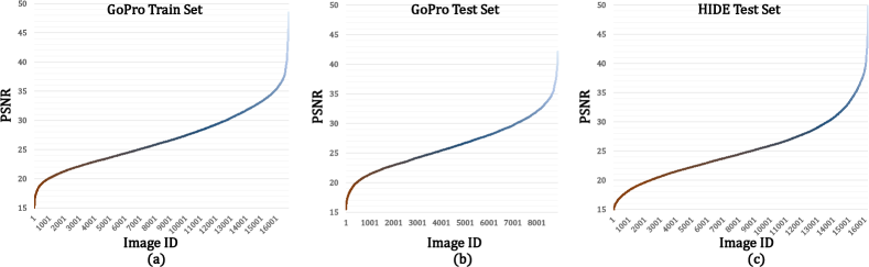
Figure 9: Distribution of GoPro [25] and HIDE [29] Dataset. (a) The ranked PSNR curve of the image patches from GoPro train set; (b) The ranked PSNR curve of the image patches from GoPro test set; (c) The ranked PSNR curve of the image patches from HIDE test set.

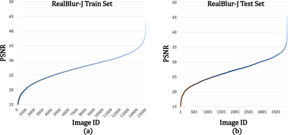
Figure 10: Distribution of RealBlur-J [27] Dataset. (a) The ranked PSNR curve of the image patches from RealBlur-J train set; (b) The ranked PSNR curve of the image patches from RealBlur-J test set.

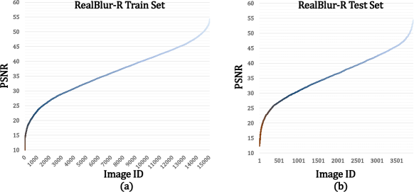
Figure 11: Distribution of RealBlur-R [27] Dataset. (a) The ranked PSNR curve of the image patches from RealBlur-R train set; (b) The ranked PSNR curve of the image patches from RealBlur-R test set.

Dataset Distribution

Figs. 9 - 11 shows the distribution of the blur patches from different dataset. As indicated in Fig. 9 and Fig. 10, the degraded patches from GoPro, HIDE and RealBlur-J dataset are almost all fall within the range of [15 dB, 45 dB]. Thus, we group the patches to 6 degradation degrees: ($\leq$ 20 dB, $\tilde{c}=1$), ($\leq$ 25 dB, $\tilde{c}=2$), ($\leq$ 30 dB, $\tilde{c}=3$), ($\leq$ 35 dB, $\tilde{c}=4$), ($\leq$ 40 dB, $\tilde{c}=5$) and ($>$ 40 dB, $\tilde{c}=6$) for the classifier training. Different from other dataset, the degraded patches from RealBlur-R are almost all fall in the range of [15 dB, 55 dB] (shown in Fig. 11). Thus, we group the patches from RealBlur-R to 8 degradation degrees: ($\leq$ 20 dB, $\tilde{c}=1$), ($\leq$ 25 dB, $\tilde{c}=2$), ($\leq$ 30 dB, $\tilde{c}=3$), ($\leq$ 35 dB, $\tilde{c}=4$), ($\leq$ 40 dB, $\tilde{c}=5$), ($\leq$ 45 dB, $\tilde{c}=6$), ($\leq$ 50 dB, $\tilde{c}=7$) and ($>$ 50 dB, $\tilde{c}=8$) for the classifier training.

Clustering Criteria

We split the image patches into different classes according to PSNR, which is a direct and efficient measure of degradation degree. We conduct experiments: ① In paper, we apply a step ($\gamma$) of 5 dB to cluster the blur patches into 6 degradation degrees from 15 dB to 45 dB. Here we change $\gamma$ within the range of $[3,4,5,6,10]$, and obtain almost the same PSNRs (34.50 dB). Classification accuracies and utilization rates of the sub-decoders (D-rates) are (83.7%, 87.2%), (87.0%, 86.0%), (89.8%, 84.3%), (91.4%, 87.7%), and (94.6%, 84.8%) respectively. First, although the larger step acquires better classification accuracy, AdaRevD-B ($4$ sub-decoders) has a big tolerance for accuracy corresponding to a small $\gamma$ (e.g., $9$ classes when $\gamma=3$). Second, it is observed that almost all the misclassified patches are classified to the adjacent degradation degree, shown in Table 8 ($\gamma=5$). Only a few patches would exit at earlier sub-decoder (slightly reduce PSNR of the whole image), while a few exit at later sub-decoder (slightly increase PSNR), which have certain complementary effects on the final PSNR. ② Following ClassSR [16], we separate PSNRs into 6 classes with the same numbers of blur patches, the PSNR is also the same (34.50 dB), even with lower classification accuracy (85.1%). Thus, AdaRevD does not demand a very high classification accuracy, and it is acceptable that a small number of patches are classified to adjacent degradation degree.

Evaluation Metric

The computational complexity of MACs (G) and the number of parameters (M) are reported in Table 9. Table 9 illustrates that our method can further explore the well-trained NAFNet’s [5] insufficient decoding capability (33.69 dB) to a higher level (34.10 dB), which is similar to UFPNet [10] (34.06 dB 243 G), but with fewer MACs (168 G).

Early-exit Signal

In AdaRevD, early-exit signal $E_{c}$ is determined by $\mathbf{O}_{c}^{j}$ and $\tau$. The $\mathbf{O}_{c}^{j}$ of RevD-B on GoPro, RealBlur-J and RealBlur-R datasets are summarized in Tables 10, 11 and 12. Furthermore, the $\mathbf{O}_{c}^{j}$ of RevD-L on these three datasets are shown in Tables 13, 14 and 15. The first $\mathbf{O}_{c}^{j-1}$ where its next $\mathbf{O}_{c}^{j}$ is smaller than $\tau=0.05$ (the patch exit in the ($(j-1)$th sub-decoder) is highlighted in the tables.

As illustrated in these tables, blur patches with varying degradation degrees exhibit distinct improvements in PSNR within the same sub-decoder. The higher the PSNR, the less restoration the patch undergoes in the identical sub-decoder. As more sub-decoders are progressively stacked, the model’s capacity to recover images reaches saturation. Tables 10 and 13 demonstrate that the $E_{c}$ remains consistent between the training set and test set when $\tau=0.05$. Moreover, the performance of the various sud-decoders on the train and test set in the tables indicate that selecting the early-exit signal $E_{c}$ based on the train set ensures effective recovery of patches from the test set. In essence, opting for $E_{c}$ from the train set is rational, as the sub-decoder saturation observed in the train set aligns with the saturation observed in the test set.

8 Viasulizations

The visual results for GoPro [25], HIDE [29], RealBlur-R [27] and RealBlur-J [27] are presented in Figs. 12, 13, 14 and 15, respectively. The visualizations depicted in Fig. 12 and Fig. 13 illustrate AdaRevD’s capability to restore sharper images. We also show the visualization results on the RealBlur [27] dataset in Fig. 14 and Fig. 15. It can be observed that our model yields more visually pleasant outputs than other methods on both synthetic and real-world motion deblurring. This is evident when compared to other SOTA methods, such as DeepRFT [24] and UFPNet [10].

Table 13: Improvement of diffent sub-decoders in RevD-L on GoPro dataset.

	TrainSet								TestSet
Degree	dec1	dec2	dec3	dec4	dec5	dec6	dec7	dec8	dec1	dec2	dec3	dec4	dec5	dec6	dec7	dec8
$\leq$20	11.068	0.601	0.257	0.222	0.198	0.109	0.047	0.014	10.201	0.610	0.252	0.269	0.198	0.107	0.048	0.015
20-25	10.903	0.400	0.154	0.135	0.118	0.064	0.026	0.007	9.569	0.345	0.129	0.153	0.122	0.055	0.021	0.007
25-30	9.141	0.227	0.076	0.070	0.060	0.031	0.012	0.003	8.053	0.206	0.065	0.073	0.064	0.030	0.009	0.003
30-35	6.176	0.145	0.037	0.035	0.029	0.015	0.007	0.002	5.362	0.125	0.030	0.041	0.031	0.015	0.005	0.002
35-40	3.437	0.101	0.019	0.018	0.014	0.007	0.004	0.001	2.798	0.116	0.012	0.023	0.016	0.010	0.003	0.001
$>$40	2.365	0.057	0.016	0.010	0.007	0.007	0.008	0.002	1.470	0.067	0.013	0.018	0.014	0.006	0.003	0.001

Table 14: Improvement of diffent sub-decoders in RevD-L on RealBlur-J dataset.

	TrainSet								TestSet
Degree	dec1	dec2	dec3	dec4	dec5	dec6	dec7	dec8	dec1	dec2	dec3	dec4	dec5	dec6	dec7	dec8
$\leq$20	11.718	0.788	0.429	0.227	0.221	0.131	0.101	0.006	5.131	0.074	0.065	0.052	0.056	0.032	0.022	0.002
20-25	11.113	0.606	0.330	0.190	0.161	0.082	0.066	0.004	4.813	0.125	0.092	0.050	0.056	0.033	0.024	0.002
25-30	9.956	0.419	0.218	0.133	0.096	0.045	0.039	0.003	4.119	0.089	0.067	0.045	0.037	0.019	0.014	0.001
30-35	8.348	0.263	0.129	0.082	0.050	0.022	0.025	0.002	3.486	0.066	0.038	0.028	0.021	0.009	0.010	0.001
35-40	7.040	0.186	0.091	0.048	0.029	0.0159	0.019	0.002	2.444	0.052	0.050	0.032	0.013	0.004	0.006	0.000
$>$40	5.444	0.158	0.081	0.039	0.022	0.014	0.018	0.001	1.462	-0.021	-0.018	0.026	-0.021	0.007	0.003	-0.003

Table 15: Improvement of diffent sub-decoders in RevD-L on RealBlur-R dataset.

	TrainSet								TestSet
Degree	dec1	dec2	dec3	dec4	dec5	dec6	dec7	dec8	dec1	dec2	dec3	dec4	dec5	dec6	dec7	dec8
$\leq$20	12.037	1.174	0.357	0.105	0.188	0.117	0.029	0.000	5.524	0.178	0.062	0.033	0.062	0.032	0.010	0.000
20-25	11.988	1.102	0.314	0.098	0.174	0.098	0.024	0.000	5.252	0.227	0.062	0.037	0.064	0.023	0.007	0.000
25-30	11.895	1.030	0.259	0.079	0.132	0.070	0.019	0.000	5.611	0.214	0.062	0.036	0.046	0.021	0.006	0.000
30-35	11.260	0.891	0.215	0.060	0.094	0.055	0.017	0.000	4.190	0.190	0.041	0.023	0.032	0.016	0.005	0.000
35-40	9.419	0.640	0.136	0.035	0.055	0.038	0.013	0.000	3.372	0.189	0.037	0.019	0.026	0.017	0.006	0.000
40-45	7.243	0.424	0.085	0.022	0.030	0.027	0.009	0.000	3.016	0.141	0.031	0.016	0.018	0.016	0.004	0.000
45-50	5.093	0.259	0.044	0.013	0.014	0.015	0.005	0.000	1.991	0.058	0.020	0.007	0.006	0.008	0.003	0.000
$>$50	3.139	0.183	0.020	0.008	0.006	0.007	0.003	0.000	1.128	-0.014	0.010	0.007	0.003	0.008	0.002	0.000

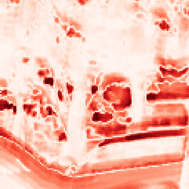
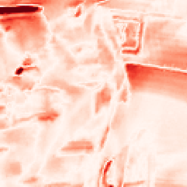
(a) Blur

(b) DeepRFT+[24]

(c) NAFNet64 [5]

(d) UFPNet[10]

(e) AdaRevD-B

(f) AdaRevD-L

(g) Sharp

Figure 12: Examples on the GoPro test dataset. The odd rows show blur image, predicted images of different methods, and ground-truth sharp image. The even rows show the residual of the blur image / predicted sharp images and the ground-truth sharp image.

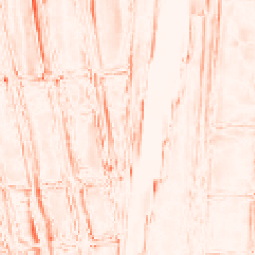
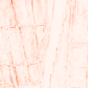
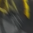
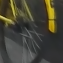
(a) Blur

(b) DeepRFT+[24]

(c) NAFNet64 [5]

(d) UFPNet[10]

(e) AdaRevD-B

(f) AdaRevD-L

(g) Sharp

Figure 13: Examples on the HIDE test dataset.

(a) Blur

(b) DeepRFT+ [24]

(c) Stripformer [32]

(d) UFPNet [10]

(e) AdaRevD-B

(f) AdaRevD-L

(g) Sharp

Figure 14: Examples on the RealBlur-J test dataset.

(a) Blur

(b) DeepRFT+ [24]

(c) Stripformer [32]

(d) UFPNet [10]

(e) AdaRevD-B

(f) AdaRevD-L

(g) Sharp

Figure 15: Examples on the RealBlur-R test dataset.

References

- Ba et al. [2016] Lei Jimmy Ba, Jamie Ryan Kiros, and Geoffrey E. Hinton. Layer normalization. CoRR, abs/1607.06450, 2016.
- Cai et al. [2020] Han Cai, Chuang Gan, Tianzhe Wang, Zhekai Zhang, and Song Han. Once for all: Train one network and specialize it for efficient deployment. In Proc. ICLR, 2020.
- Cai et al. [2023] Yuxuan Cai, Yizhuang Zhou, Qi Han, Jianjian Sun, Xiangwen Kong, Jun Li, and Xiangyu Zhang. Reversible column networks. In Proc. ICLR, 2023.
- Chen et al. [2021] Liangyu Chen, Xin Lu, Jie Zhang, Xiaojie Chu, and Chengpeng Chen. Hinet: Half instance normalization network for image restoration. In Proc. CVPR Workshop, 2021.
- Chen et al. [2022] Liangyu Chen, Xiaojie Chu, Xiangyu Zhang, and Jian Sun. Simple baselines for image restoration. In Proc. ECCV, 2022.
- Chiley et al. [2023] Vitaliy Chiley, Vithursan Thangarasa, Abhay Gupta, Anshul Samar, Joel Hestness, and Dennis DeCoste. Revbifpn: The fully reversible bidirectional feature pyramid network. In Proc. MLSys, 2023.
- Cho et al. [2021] Sung-Jin Cho, Seo-Won Ji, Jun-Pyo Hong, Seung-Won Jung, and Sung-Jea Ko. Rethinking coarse-to-fine approach in single image deblurring. In Proc. ICCV, 2021.
- Chu et al. [2022] Xiaojie Chu, Liangyu Chen, Chengpeng Chen, and Xin Lu. Improving image restoration by revisiting global information aggregation. In Proc. ECCV, 2022.
- Dong et al. [2023] Jiangxin Dong, Jinshan Pan, Zhongbao Yang, and Jinhui Tang. Multi-scale residual low-pass filter network for image deblurring. In Proc. ICCV, 2023.
- Fang et al. [2023] Zhenxuan Fang, Fangfang Wu, Weisheng Dong, Xin Li, Jinjian Wu, and Guangming Shi. Self-supervised non-uniform kernel estimation with flow-based motion prior for blind image deblurring. In Proc. CVPR, 2023.
- Gomez et al. [2017] Aidan N Gomez, Mengye Ren, Raquel Urtasun, and Roger B Grosse. The reversible residual network: Backpropagation without storing activations. In Proc. NeurIPS, 2017.
- He et al. [2016] Kaiming He, Xiangyu Zhang, Shaoqing Ren, and Jian Sun. Deep residual learning for image recognition. In Proc. CVPR, 2016.
- Jacobsen et al. [2018] Jörn-Henrik Jacobsen, Arnold WM Smeulders, and Edouard Oyallon. i-revnet: Deep invertible networks. In Proc. ICLR, 2018.
- Jin et al. [2020] Qing Jin, Linjie Yang, and Zhenyu Liao. Adabits: Neural network quantization with adaptive bit-widths. In Proc. CVPR, 2020.
- Kong et al. [2023] Lingshun Kong, Jiangxin Dong, Jianjun Ge, Mingqiang Li, and Jinshan Pan. Efficient frequency domain-based transformers for high-quality image deblurring. In Proc. CVPR, 2023.
- Kong et al. [2021] Xiangtao Kong, Hengyuan Zhao, Yu Qiao, and Chao Dong. Classsr: A general framework to accelerate super-resolution networks by data characteristic. In Proc. CVPR, 2021.
- Kornblith et al. [2019] Simon Kornblith, Mohammad Norouzi, Honglak Lee, and Geoffrey Hinton. Similarity of neural network representations revisited. In Proc. ICML, 2019.
- Kupyn et al. [2018] Orest Kupyn, Volodymyr Budzan, Mykola Mykhailych, Dmytro Mishkin, and Jiri Matas. Deblurgan: Blind motion deblurring using conditional adversarial networks. In Proc. CVPR, 2018.
- Kupyn et al. [2019] Orest Kupyn, Tetiana Martyniuk, Junru Wu, and Zhangyang Wang. Deblurgan-v2: Deblurring (orders-of-magnitude) faster and better. In Proc. ICCV, 2019.
- Li et al. [2022] Dasong Li, Yi Zhang, Ka Chun Cheung, Xiaogang Wang, Hongwei Qin, and Hongsheng Li. Learning degradation representations for image deblurring. In Proc. ECCV, 2022.
- Lin et al. [2019] Jen-Chun Lin, Wen-Li Wei, Tyng-Luh Liu, C.-C. Jay Kuo, and Hong-Yuan Mark Liao. Tell me where it is still blurry: Adversarial blurred region mining and refining. In Proc. ACM MM, 2019.
- Liu et al. [2020] Ming Liu, Zhilu Zhang, Liya Hou, Wangmeng Zuo, and Lei Zhang. Deep adaptive inference networks for single image super-resolution. In Proc. ECCV, 2020.
- Mangalam et al. [2022] Karttikeya Mangalam, Haoqi Fan, Yanghao Li, Chao-Yuan Wu, Bo Xiong, Christoph Feichtenhofer, and Jitendra Malik. Reversible vision transformers. In Proc. CVPR, 2022.
- Mao et al. [2023] Xintian Mao, Yiming Liu, Fengze Liu, Qingli Li, Wei Shen, and Yan Wang. Intriguing findings of frequency selection for image deblurring. In Proc. AAAI, 2023.
- Nah et al. [2017] Seungjun Nah, Tae Hyun Kim, and Kyoung Mu Lee. Deep multi-scale convolutional neural network for dynamic scene deblurring. In Proc. CVPR, 2017.
- Park et al. [2020] Dongwon Park, Dong Un Kang, Jisoo Kim, and Se Young Chun. Multi-temporal recurrent neural networks for progressive non-uniform single image deblurring with incremental temporal training. In Proc. ECCV, 2020.
- Rim et al. [2020] Jaesung Rim, Haeyun Lee, Jucheol Won, and Sunghyun Cho. Real-world blur dataset for learning and benchmarking deblurring algorithms. In Proc. ECCV, 2020.
- Ronneberger et al. [2015] Olaf Ronneberger, Philipp Fischer, and Thomas Brox. U-net: Convolutional networks for biomedical image segmentation. In Proc. MICCAI, 2015.
- Shen et al. [2019] Ziyi Shen, Wenguan Wang, Xiankai Lu, Jianbing Shen, Haibin Ling, Tingfa Xu, and Ling Shao. Human-aware motion deblurring. In Proc. ICCV, 2019.
- Tan et al. [2020] Mingxing Tan, Ruoming Pang, and Quoc V Le. Efficientdet: Scalable and efficient object detection. In Proc. CVPR, 2020.
- Tao et al. [2018] Xin Tao, Hongyun Gao, Xiaoyong Shen, Jue Wang, and Jiaya Jia. Scale-recurrent network for deep image deblurring. In Proc. CVPR, 2018.
- Tsai et al. [2022] Fu-Jen Tsai, Yan-Tsung Peng, Yen-Yu Lin, Chung-Chi Tsai, and Chia-Wen Lin. Stripformer: Strip transformer for fast image deblurring. In ECCV, 2022.
- Tu et al. [2022] Zhengzhong Tu, Hossein Talebi, Han Zhang, Feng Yang, Peyman Milanfar, Alan Bovik, and Yinxiao Li. Maxim: Multi-axis mlp for image processing. In Proc. CVPR, 2022.
- Vaswani et al. [2017] Ashish Vaswani, Noam Shazeer, Niki Parmar, Jakob Uszkoreit, Llion Jones, Aidan N Gomez, Łukasz Kaiser, and Illia Polosukhin. Attention is all you need. 2017.
- Wang et al. [2022a] Shizun Wang, Jiaming Liu, Kaixin Chen, Xiaoqi Li, Ming Lu, and Yandong Guo. Adaptive patch exiting for scalable single image super-resolution. In Proc. ECCV, 2022a.
- Wang et al. [2022b] Zhendong Wang, Xiaodong Cun, Jianmin Bao, and Jianzhuang Liu. Uformer: A general u-shaped transformer for image restoration. In Proc. CVPR, 2022b.
- Whang et al. [2022] Jay Whang, Mauricio Delbracio, Hossein Talebi, Chitwan Saharia, Alexandros G. Dimakis, and Peyman Milanfar. Deblurring via stochastic refinement. In Proc. CVPR, 2022.
- Yang et al. [2020] Taojiannan Yang, Sijie Zhu, Chen Chen, Shen Yan, Mi Zhang, and Andrew Willis. Mutualnet: Adaptive convnet via mutual learning from network width and resolution. In Proc. ECCV, 2020.
- Yu and Huang [2019a] Jiahui Yu and Thomas Huang. Autoslim: Towards one-shot architecture search for channel numbers. arXiv preprint arXiv:1903.11728, 2019a.
- Yu and Huang [2019b] Jiahui Yu and Thomas S Huang. Universally slimmable networks and improved training techniques. In Proc. ICCV, 2019b.
- Yu et al. [2018] Jiahui Yu, Linjie Yang, Ning Xu, Jianchao Yang, and Thomas Huang. Slimmable neural networks. In Proc. ICLR, 2018.
- Zamir et al. [2021] Syed Waqas Zamir, Aditya Arora, Salman H. Khan, Munawar Hayat, Fahad Shahbaz Khan, Ming-Hsuan Yang, and Ling Shao. Multi-stage progressive image restoration. In Proc. CVPR, 2021.
- Zamir et al. [2022] Syed Waqas Zamir, Aditya Arora, Salman H. Khan, Munawar Hayat, Fahad Shahbaz Khan, and Ming-Hsuan Yang. Restormer: Efficient transformer for high-resolution image restoration. In Proc. CVPR, 2022.
- Zhang et al. [2019] Hongguang Zhang, Yuchao Dai, Hongdong Li, and Piotr Koniusz. Deep stacked hierarchical multi-patch network for image deblurring. In Proc. CVPR, 2019.
- Zhang et al. [2020] Kaihao Zhang, Wenhan Luo, Yiran Zhong, Lin Ma, Björn Stenger, Wei Liu, and Hongdong Li. Deblurring by realistic blurring. In Proc. CVPR, 2020.