Jacobian-Enhanced Neural Networks

Abstract

Jacobian-Enhanced Neural Networks (JENN) are densely connected multi-layer perceptrons, whose training process is modified to predict partial derivatives accurately. Their main benefit is better accuracy with fewer training points compared to standard neural networks. These attributes are particularly desirable in the field of computer-aided design, where there is often the need to replace computationally expensive, physics-based models with fast running approximations, known as surrogate models or meta-models. Since a surrogate emulates the original model accurately in real time, it yields a computational speed benefit that can be used to carry out orders of magnitude more function calls quickly. However, in the special case of gradient-enhanced methods, there is the additional value proposition that partial derivatives are accurate, which is a critical property for one important use-case: surrogate-based optimization. This work derives the complete theory and exemplifies its superiority over standard neural nets for surrogate-based optimization.

Nomenclature

$L$	number of layers in neural network
$a$	activation output, $a=g(z)$
$b$	bias (parameter to be learned)
$g$	activation function
$m$	number of training examples
$n$	number of nodes in a layer
$n_{x}$	number of nodes in input layer, $n_{x}=n^{[0]}$
$n_{y}$	number of nodes in output layer, $n_{y}=n^{[L]}$
$w$	weight (parameter to be learned)
$x$	training data input
$y$	training data output
$\hat{y}$	predicted output
$z$	linear activation input
Hyperparameters
$\alpha$	learning rate
$\beta$	hyperparameter to priorities training data values
$\gamma$	hyperparameter to priorities training data partials
$\lambda$	hyperparameter used for regularization
Mathematical Symbols and Operators
$\mathcal{J}$	cost function
$\mathcal{L}$	loss function
$()_{j}\prime$	first derivative, $\partial()/\partial x_{j}$
$()_{j}\prime\prime$	second derivative, $\partial^{2}()/\partial x_{j}^{2}$
Superscripts/Subscripts
$i$	$i^{\text{th}}$ node in current layer, $1\leq i\leq n^{[l]}$
$j$	$j^{\text{th}}$ input, $x_{j}$, $1\leq j\leq n_{x}$
$k$	$k^{\text{th}}$ output, $y_{k}$, $1\leq k\leq n_{y}$
$l$	$l^{\text{th}}$ layer of neural network, $1\leq l\leq L$
$r$	$r^{\text{th}}$ node of previous layer, $1\leq r\leq n^{[l-1]}$
$s$	$s^{\text{th}}$ node of current layer, $1\leq s\leq n^{[l]}$
$t$	$t^{\text{th}}$ training example, $1\leq t\leq m$

I Introduction

Jacobian-Enhanced Neural Networks (JENN) are fully connected multi-layer perceptrons, whose training process is modified to predict partial derivatives accurately. This is accomplished by minimizing a modified version of the Least Squares Estimator (LSE) that accounts for Jacobian prediction error, where a Jacobian extends the concept of a gradient for vector functions with more than one output. The main benefit of jacobian-enhancement (synonymous to gradient-enhancement) is better accuracy with fewer training points compared to standard fully connected neural nets. This paper develops the theory behind JENN and quantifies its benefits for the intended use-case. It complements previous work in the following ways. First, it provides a concise but complete derivation, including equations in vectorized form (see appendix), without relying on automatic differentiation. Second, it provides a deep-learning formulation that can handle any number of inputs, hidden layers, or outputs. Finally, through judicious use of hyperparameters, it enables weighting; i.e. a process by which individual sample points can be prioritized differently in situations that call for it. The latter, in particular, gives rise to the concept of polishing (described in the application section) which offers an additional tuning mechanism to further improve Surrogate-Based Optimization (SBO) in gradient-descent applications.

I-A Intended Use-Case

JENN is intended for the field of computer aided design, where there is often a need to replace computationally expensive, physics-based models with fast running approximations, commonly referred to as surrogate models or meta-models. Since a surrogate emulates the original model accurately in fractions of second, it yields a speed benefit that can be used to carry out orders of magnitude more function calls quickly. This allows designers to explore a broader tradespace, and more readily quantify the impact of various parameters in order to better understand the performance of the system under design. While this is true of any surrogate modeling approach, JENN has an additional benefit that most surrogate modeling approaches lack: the ability to predict partial derivatives with improved accuracy. This is a critical property for one important use-case: surrogate-based optimization. The field of engineering is rich in design applications of such a use-case with entire book chapters dedicated to it [1, 2, 3, 4], review papers [5, 6, 7, 8], and countless examples to be found, particularly in the field of aerospace engineering [9, 10, 11, 12].

I-B Limitations

First and foremost, gradient-enhanced methods require factors and responses to be smooth and continuous. Second, the value proposition of a surrogate is that the computational expense of generating training data to fit the model is much less than the computational expense of directly performing the analysis with the original model itself, which is not always true, especially when computing partials. Gradient-enhanced methods are therefore only beneficial if the cost of obtaining partials is not excessive in the first place (e.g. adjoint methods [13] in computational fluid dynamics), or if the need for accuracy outweighs the cost of computing the partials. One should therefore carefully weigh the benefit of gradient-enhanced methods relative to the needs of their application.

I-C Supporting Software

An open-source Python library that implements the theory can be found at https://pypi.org/project/jenn/. There exist many excellent deep learning frameworks, such as TensorFlow [14] and PyTorch [15], which are more performant and versatile than JENN, as well as many all-purpose machine learning libraries, such as scikit-learn [16]. However, gradient-enhancement is not inherently part of those popular frameworks, let alone the availability of prepared functions to predict partials after training is complete, which requires non-trivial effort to be implemented in those tools. The present library seeks to close that gap. It is intended for engineers with limited time, who have a need to predict partials accurately, and who are seeking a minimal-effort Application Programming Interface (API) with low-barrier to entry.

II Previous Work

A cursory literature research reveals that the field of gradient-enhanced regression is predominantly focused on Gaussian processes. Dedicated book chapters can be found about gradient-enhanced Kriging models [2], salient open-source libraries have been almost exclusively devoted to gradient-enhanced Bayesian methods  [17], and even review papers about gradient-enhanced meta-models only mention neural networks in passing [18]. However, early work by Sellar and Batill [19] can be found in the late 1990’s, which uses gradient-enhanced neural network approximations in the context of Concurrent Subspace Optimization (CSSO), a type of optimization architecture in the field of multi-disciplinary design optimization. They conclude that gradient-enhanced neural networks are more accurate and require significantly less training data than their non-enhanced counterparts, which seems to be the general consensus in all work surveyed for this paper.

Follow-on research by that Liu and Batill [20] provides the mathematical derivation of the equations for neural net gradient-enhancement, but the formulation is not general; it is limited to shallow neural networks with only two layers, which is of limited utility. This shortcoming is overcome by Giannakoglou et al. [10] in the late 2000’s who developed a deep neural-network formulation with gradient-enhancement and use it for aerodynamic design applications. All necessary equations to reproduce their algorithm are provided, but their formulation is limited to only one output and the vectorized form is missing for computer programming.

Recent work by Bouhlel et al. [11] in 2020 takes a different approach, relying instead on established deep-learning frameworks to delegate back-propagation to third-party, automatic-differentiation tools. Bouhlel et al. successfully apply gradient-enhanced neural networks to aerodynamic use-cases and re-affirm the previous conclusion that such techniques improve accuracy and reduce the amount of training data needed, provided the cost of obtaining the gradient is not prohibitive in the first place. While deep learning frameworks have obvious advantages (e.g. parallel computing), there is complementary research value in developing the equations for back-propagation, which is a special case of automatic differentiation for scalar functions. Stand-alone equations are reproducible without third-party tools and convey deeper insight into the mechanics behind an algorithm, which others can build upon.

The works surveyed so far have focused on prediction accuracy, but Hoffman et al. [21] take a different approach by focusing on robustness instead. They introduce the concept of Jacobian regularization for classification, where the key idea is to ensure robustness of models against input perturbations due to adversarial attacks; for example, a purposefully modified input image to avoid detection. However, robustness is outside the scope of the present work, which is to predict design partials accurately given high quality inputs.

Finally, the most recent work on gradient-enhanced neural nets focuses on gradient-enhanced Physics-Informed Neural Networks [22] (PINN). This novel research uses the residuals (and its partials) of Partial Differential Equations (PDE), governing some physical system of interest, as the loss function for training neural nets (instead of using the classic least squares estimator). However, PINN is outside the scope of the present work, which is to develop a general purpose algorithm to fit any smooth function, regardless of what it represents, even if it is not physics-informed.

III Mathematical Derivation

Jacobian-Enhanced Neural Networks (JENN) follow the same steps as standard Neural Networks (NN), shown in Fig. 1, except that the cost function used during parameter update is modified to account for partial derivatives, with the consequence that back propagation must be modified accordingly. This section provides the mathematical derivation for Jacobian-enhancement.

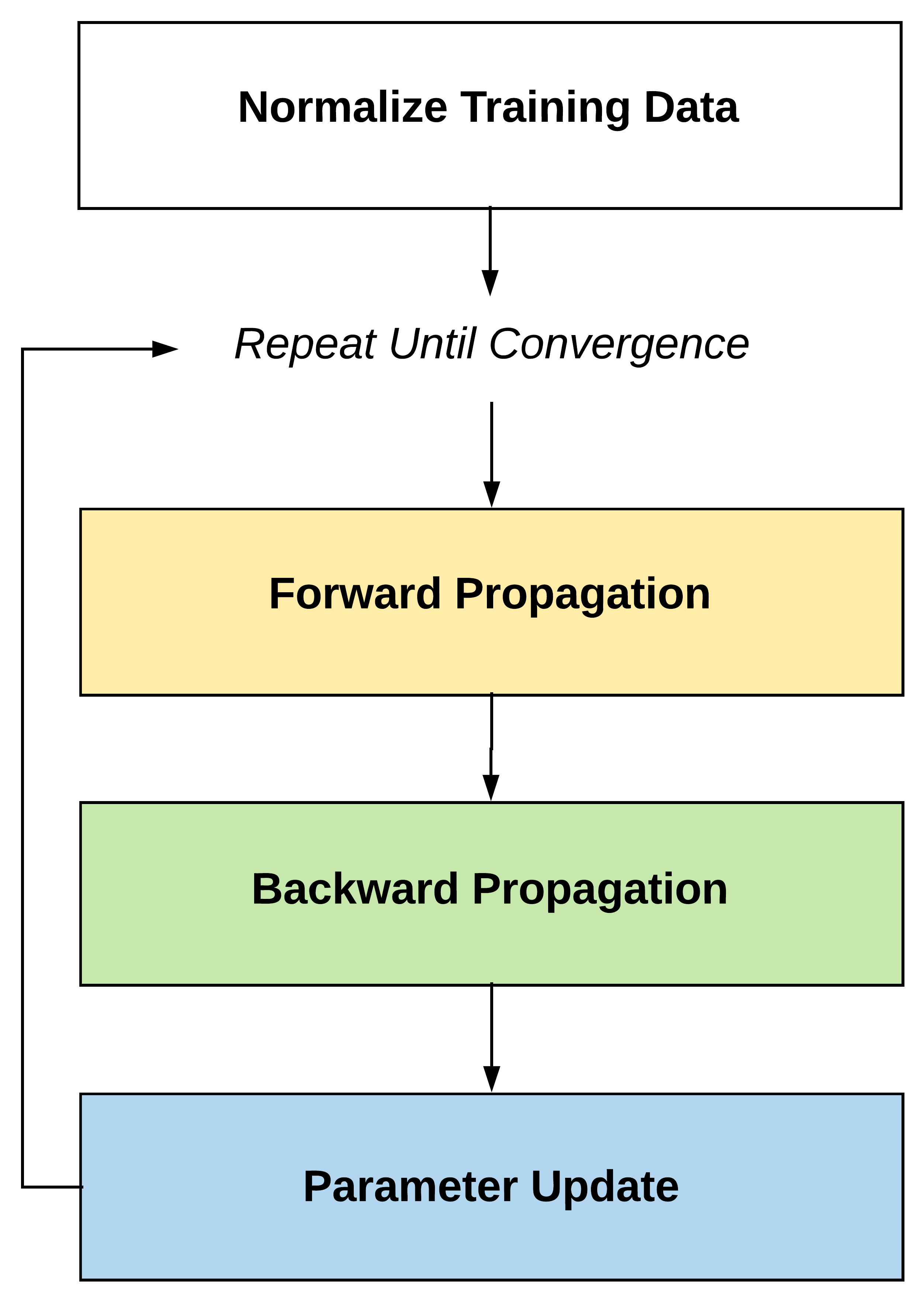
Figure 1: summary of neural net training process

III-A Notation

For clarity, let us adopt a similar notation to the one used by Andrew Ng [23] where superscript $l$ denotes the layer number, $t$ is the training example, and subscript $i$ indicates the node number in a layer. For instance, the activation of the $i^{\text{th}}$ node in layer $l$ evaluated at example $t$ would be denoted:

$$a_{i}^{[l](t)}=g\left(z_{i}^{[l](t)}\right)\quad\begin{cases}\forall~{}i\in\{1,\dots,n^{[l]}\}\\ \forall~{}l\in\{1,\dots,L\}\\ \forall~{}t\in\{1,\dots,m\}\end{cases}$$

To avoid clutter in the derivation to follow, it will be understood that subscripts $s$ and $r$ refer to quantities associated with the current and previous layer, respectively, evaluated at example $t$ without the need for superscripts. Concretely:

$$a_{s} \equiv a_{i=s}^{[l](t)}\quad z_{s} \equiv z_{i=s}^{[l](t)}~{} \forall~{}s\in\{1,\dots,n^{[l]}\}$$ (1a)

$$a_{r} \equiv a_{i=r}^{[l-1](t)}\quad z_{r} \equiv z_{i=r}^{[l-1](t)}~{} \forall~{}r\in\{1,\dots,n^{[l-1]}\}$$ (1b)

Derivatives with respect to input $x_{j}$ are denoted by the prime symbol and subscript $j$. For example:

$$a_{s_{j}}^{\prime} \equiv\left(\dfrac{\partial a_{s}}{\partial x_{j}}\right)\qquad z_{s_{j}}^{\prime} \equiv\left(\dfrac{\partial z_{s}^{[l]}}{\partial x_{j}}\right)$$

In turn, vector quantities will be defined in bold font. For instance, the input and output layers associated with example $t$ would be given by:

$$\boldsymbol{a}^{[1](t)}=\boldsymbol{x}^{(t)}=\left[\begin{matrix}x_{1}^{(t)}\\ \vdots\\ x_{n_{x}}^{(t)}\end{matrix}\right]\quad\boldsymbol{y}^{(t)}=\left[\begin{matrix}{y}_{1}^{(t)}\\ \vdots\\ {y}_{n_{y}}^{(t)}\end{matrix}\right]=\boldsymbol{a}^{[L](t)}$$

III-B Normalize Training Data

Normalizing the training data can greatly improve performance when either inputs or outputs differ by orders of magnitude. A simple way to improve numerical conditioning is to subtract the mean $\mu$ and divide by the standard deviation $\sigma$ of the data. The normalized data then becomes:

$$\boldsymbol{x}^{(t)} :=\frac{\boldsymbol{x}^{(t)}-\boldsymbol{\mu}_{x}}{\boldsymbol{\sigma}_{x}}~{}\in~{}\mathbb{R}^{n_{x}}$$ (2a)

$$\boldsymbol{y}^{(t)} :=\frac{\boldsymbol{y}^{(t)}-\boldsymbol{\mu}_{y}}{\boldsymbol{\sigma}_{y}}~{}\in~{}\mathbb{R}^{n_{y}}$$ (2b)

$${y}_{k_{j}}^{\prime(t)} :=\left(\frac{\partial y_{k}}{\partial x_{j}}\right)^{(t)}\times\frac{\sigma_{x_{j}}}{{\sigma}_{y_{k}}}~{}\in~{}\mathbb{R}$$ (2c)

This approach works well, except when all values are very close such that the denominator vanishes as standard deviation goes to zero. In that case, alternative normalization methods (or none) should be considered.

III-C Forward Propagation

Predictions are obtained by propagating information forward throughout the neural network in a recursive manner, starting with the input layer and ending with the output layer. For each layer (excluding input layer), activations are computed as:

$$a_{s}=g(z_{s}) z_{s}=w_{sr}a_{r}+b_{s}$$ (3a)

$$a_{s_{j}}^{\prime}=g^{\prime}(z_{s})z_{s_{j}}^{\prime} z_{s_{j}}^{\prime}=w_{sr}a_{r_{j}}^{\prime}$$ (3b)

where $\left\{w_{sr},b_{s}\right\}$ are neural network parameters to be learned. For the hidden layers ($1<l<L$), the activation function is taken to be the hyperbolic tangent:

$$g(z) =\frac{e^{z}-e^{-z}}{e^{z}+e^{-z}}$$ (4a)

$$g^{\prime}(z) \equiv\frac{\partial g}{\partial z}=1-g(z)^{2}$$ (4b)

$$g^{\prime\prime}(z) \equiv\frac{\partial^{2}g}{\partial z^{2}}=-2g(z)g(z)^{\prime}$$ (4c)

For the output layer ($l=L$), the activation function is linear:

$$g(z)=z\quad\Rightarrow\quad g^{\prime}(z)=1\quad\Rightarrow\quad g^{\prime\prime}(z)=0$$ (5)

III-D Parameter Update

The neural network parameters are learned by solving the following, unconstrained optimization problem:

$$\theta^{*}=\arg\underset{\theta}{\min}~{}\mathcal{J(\theta)}\quad\forall\quad\theta\in\left\{w_{sr},b_{s}\right\}$$ (6)

where it should be understood that $\left\{w_{sr},b_{s}\right\}$ is short hand for all parameters of the neural network. The cost function $\mathcal{J}$ is given by the following expression, where $\lambda$ is a hyper-parameter to be tuned which controls regularization:

$$\mathcal{J(\theta)} =\frac{1}{m}\sum_{t=1}^{m}\mathcal{L}^{(t)}+\frac{\lambda}{2m}\sum_{l=2}^{L}\sum_{s=1}^{n^{[l]}}\sum_{r=1}^{n^{[l-1]}}w_{sr}^{2}$$ (7)

Parameters are updated iteratively using gradient-descent:

$$\theta :=\theta-\alpha\frac{\partial\mathcal{J}}{\partial\theta}$$ (8)

where the hyper-parameter $\alpha$ is the learning rate. In practice, some improved version of gradient-descent would be used instead, such as ADAM [24], but the former is easier to explain without loss of generality. The loss function $\mathcal{L}$ is taken to be a modified version of the Least rquares Estimator (LSE), augmented with an extra term to account for partial derivatives:

$$\mathcal{L}^{(t)}=\frac{1}{2} \sum_{s=1}^{n_{y}}\beta_{s}^{(t)}\left(a_{s}^{[L](t)}-y_{s}^{(t)}\right)^{2}\dots$$

$$\dots+\frac{1}{2}\sum_{s=1}^{n_{y}}\sum_{j=1}^{n_{x}}\gamma_{s_{j}}^{(t)}\left(a_{s_{j}}^{\prime[L](t)}-y_{s_{j}}^{\prime(t)}\right)^{2}$$ (9)

Note that two more hyper-parameters have been introduced: $\beta^{(t)}$ and $\gamma^{(t)}$. They act as weights that can be used to prioritize subsets of the training data in situations that call for it. By default, $\beta_{s}^{(t)}=\gamma_{s_{j}}^{(t)}=1$, meaning that all data is prioritized equally, which is the common use-case. However, in some situations, there may be an incentive to prioritize certain examples over others, as will be shown in the results section. This formulation offers the flexibility to do so.

III-E Backward Propagation

Forward propagation seeks to compute the gradient of the predicted outputs $\hat{\boldsymbol{y}}$ with respect to (abbreviated w.s.t.) the inputs $\boldsymbol{x}$. By contrast, back-propagation computes the gradient of the cost function $\mathcal{J}$ with respect to the neural net parameters $\theta$:

$$\frac{\partial\mathcal{J}}{\partial\theta} =\frac{1}{m}\sum_{t=1}^{m}\frac{\partial\mathcal{L}}{\partial\theta}^{(t)}+\frac{\lambda}{2m}\sum_{l=2}^{L}\sum_{s=1}^{n^{[l]}}\sum_{r=1}^{n^{[l-1]}}\frac{\partial}{\partial\theta}\left(w_{sr}^{2}\right)$$ (10)

III-E1 Loss Function Derivatives w.s.t. Neural Net Parameters

In a first step, assume the quantities ${\partial\mathcal{L}}/{\partial a_{s}}$ and ${\partial\mathcal{L}}/{\partial a^{\prime}_{s_{j}}}$ are known and consider the gradient of the loss function $\mathcal{L}$ with respect to the parameters $\theta$ from layer $l$. Applying the chain rule to Eq. III-D yields:

$$\frac{\partial\mathcal{L}}{\partial\theta}=\frac{\partial\mathcal{L}}{\partial a_{s}}\frac{\partial a_{s}}{\partial z_{s}}\frac{\partial z_{s}}{\partial\theta}+\sum_{j=1}^{n_{x}}\frac{\partial\mathcal{L}}{\partial a^{\prime}_{s_{j}}}\left(\frac{\partial a^{\prime}_{s_{j}}}{\partial z_{s}}\frac{\partial z_{s}}{\partial\theta}+\frac{\partial a^{\prime}_{s_{j}}}{\partial z^{\prime}_{s_{j}}}\frac{\partial z^{\prime}_{s_{j}}}{\partial\theta}\right)$$ (11)

where the superscript $t$ has been dropped for notational convenience, with the understanding that all equations to follow apply to example $t$. The various partial derivatives in Eq. 11 follow from Eq. 3:

$$\frac{\partial a_{s}}{\partial z_{s}}=g^{\prime}(z_{s})\quad \frac{\partial a_{s_{j}}^{\prime}}{\partial z_{s}}=g^{\prime\prime}(z_{s})z_{s_{j}}^{\prime}\quad \frac{\partial a_{s_{j}}^{\prime}}{\partial z_{s_{j}}^{\prime}}=g^{\prime}(z_{s})$$ (12)

$$\theta=w_{sr}:\quad \frac{\partial z_{s}}{\partial\theta}=a_{r}\quad \frac{\partial z^{\prime}_{s_{j}}}{\partial\theta}=a_{r_{j}}^{\prime}$$ (13)

$$\theta=b_{s}:\quad \frac{\partial z_{s}}{\partial\theta}=1\quad \frac{\partial z^{\prime}_{s_{j}}}{\partial\theta}=0$$ (14)

rubstituting these expressions into Eq. 11 yields:

$$\frac{\partial\mathcal{L}}{\partial w_{sr}} =\frac{\partial\mathcal{L}}{\partial a_{s}}g^{\prime}(z_{s})a_{r}~{}\dots$$

$$\dots+\sum_{j=1}^{n_{x}}\frac{\partial\mathcal{L}}{\partial a^{\prime}_{s_{j}}}\Bigl{(}g^{\prime\prime}(z_{s})z_{s_{j}}^{\prime}a_{r}+g^{\prime}(z_{s})a_{r_{j}}^{\prime}\Bigr{)}$$ (15a)

$$\frac{\partial\mathcal{L}}{\partial b_{s}} =\frac{\partial\mathcal{L}}{\partial a_{s}}g^{\prime}(z_{s})+\sum_{j=1}^{n_{x}}\frac{\partial\mathcal{L}}{\partial a^{\prime}_{s_{j}}}g^{\prime\prime}(z_{s})z_{s_{j}}^{\prime}$$ (15b)

III-E2 Loss Function Derivatives w.s.t. to Neural Net Activations

All quantities in Eq. 15 are known, except for ${\partial\mathcal{L}}/{\partial a_{s}}$ and ${\partial\mathcal{L}}/{\partial a_{s_{j}}^{\prime}}$ which must be obtained recursively by propagating information backwards from one layer to the next, starting with the output layer $L$. From Eq. III-D, it follows that:

$$\frac{\partial\mathcal{L}}{\partial a_{s}}^{[L]} =\beta_{s}\left(a_{s}-y_{s}\right)$$ (16a)

$$\frac{\partial\mathcal{L}}{\partial a_{s_{j}}^{\prime}}^{[L]} =\gamma_{s_{j}}\left(a_{s_{j}}^{\prime}-y_{s}^{\prime}\right)$$ (16b)

The derivatives for the next layer are obtained through the chain rule. According to Eq. III-D, the loss function $\mathcal{L}$ depends on $n^{[l]}$ activations $a_{s}$ and $n_{x}\times n^{[l]}$ associated partials $a_{s_{j}}^{\prime}$, which are themselves functions of $a_{r}$ and $a_{r_{j}}^{\prime}$. Hence, according to the chain rule, current layer derivatives w.s.t. to previous layer activations are:

$$\frac{\partial\mathcal{L}}{\partial a_{r}}^{[l]} =\sum_{s=1}^{n^{[l]}}\left[\frac{\partial\mathcal{L}}{\partial a_{s}}\frac{\partial a_{s}}{\partial a_{r}}+\sum_{j=1}^{n_{x}}\frac{\partial\mathcal{L}}{\partial a_{r_{j}}^{\prime}}\frac{\partial a_{r_{j}}^{\prime}}{\partial a_{r}}\right]\quad \forall~{}l=L,\dots,2$$ (17a)

$$\frac{\partial\mathcal{L}}{\partial a^{\prime}_{r_{j}}}^{[l]} =\sum_{s=1}^{n^{[l]}}\left[\frac{\partial\mathcal{L}}{\partial a_{s}}\frac{\partial a_{s}}{\partial a^{\prime}_{r_{j}}}+\sum_{j=1}^{n_{x}}\frac{\partial\mathcal{L}}{\partial a_{s_{j}}^{\prime}}\frac{\partial a_{s_{j}}^{\prime}}{\partial a^{\prime}_{r_{j}}}\right]\quad \forall~{}l=L,\dots,2$$ (17b)

Further applying the chain rule to the intermediate quantities and using Eq. 3, one finds that:

$$\frac{\partial a_{s}}{\partial a_{r}} =\frac{\partial a_{s}}{\partial z_{s}}\frac{\partial z_{s}}{\partial a_{r}}+\frac{\partial a_{s}}{\partial z_{s_{j}}^{\prime}}\cancelto{0}{\frac{\partial z_{s_{j}}^{\prime}}{\partial a_{r}}}=g^{\prime}(z_{s})w_{sr}$$ (18a)

$$\frac{\partial a_{s}}{\partial a^{\prime}_{r_{j}}} =\cancelto{0}{\frac{\partial a_{s}}{\partial z_{s}}}\frac{\partial z_{s}}{a^{\prime}_{r_{j}}}+\cancelto{0}{\frac{\partial a_{s}}{\partial z_{s_{j}}^{\prime}}}\frac{\partial z_{s_{j}}^{\prime}}{a^{\prime}_{r_{j}}}=0$$ (18b)

$$\frac{\partial a_{s_{j}}^{\prime}}{\partial a_{r}} =\frac{\partial a_{s_{j}}^{\prime}}{\partial z_{s}}\frac{\partial z_{s}}{\partial a_{r}}+\frac{\partial a_{s_{j}}^{\prime}}{\partial z_{s_{j}}^{\prime}}\cancelto{0}{\frac{\partial z_{s_{j}}^{\prime}}{\partial a_{r}}}=g^{\prime\prime}(z_{s})z_{s_{j}}^{\prime}w_{sr}$$ (18c)

$$\frac{\partial a_{s_{j}}^{\prime}}{\partial a^{\prime}_{r_{j}}} =\frac{\partial a_{s_{j}}^{\prime}}{\partial z_{s}}\cancelto{0}{\frac{\partial z_{s}}{\partial a^{\prime}_{r_{j}}}}+\frac{\partial a_{s_{j}}^{\prime}}{\partial z_{s_{j}}^{\prime}}\frac{\partial z_{s_{j}}^{\prime}}{\partial a^{\prime}_{r_{j}}}=g^{\prime}(z_{s})w_{sr}$$ (18d)

All necessary equations to compute the derivatives of the loss function w.s.t. parameters in any layer are now known. Derivatives are obtained by working our way back recursively across layers, repeatedly applying Eq. 17 after passing the solution in the current layer to the preceding layer as follows:

$$\frac{\partial\mathcal{L}}{\partial a_{s}}^{[l-1]} =\frac{\partial\mathcal{L}}{\partial a_{r}}^{[l]}$$ (19a)

$$\frac{\partial\mathcal{L}}{\partial a^{\prime}_{s_{j}}}^{[l-1]} =\frac{\partial\mathcal{L}}{\partial a^{\prime}_{r_{j}}}^{[l]}$$ (19b)

III-E3 Cost Function Derivatives w.s.t. Parameters

Putting it all together, the derivative of the cost function w.s.t. neural parameters are obtained by substituting Eq. 15 into Eq. 10, where the subscripts $s$ and $r$ are referenced to layer $l$:

$$\frac{\partial\mathcal{J}}{\partial w_{sr}} =\frac{1}{m}\sum_{t=1}^{m}\frac{\partial\mathcal{L}^{(t)}}{\partial w_{sr}}+\lambda w_{sr} \quad\forall~{}1<l\leq L$$ (20a)

$$\frac{\partial\mathcal{J}}{\partial b_{s}} =\frac{1}{m}\sum_{t=1}^{m}\frac{\partial\mathcal{L}^{(t)}}{\partial b_{s}} \quad\forall~{}1<l\leq L$$ (20b)

IV Verification and Validation

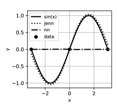
(a) $y=sin(x)$

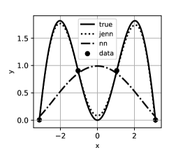
(b) $y=xsin(x)$

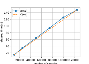
(c) Runtime

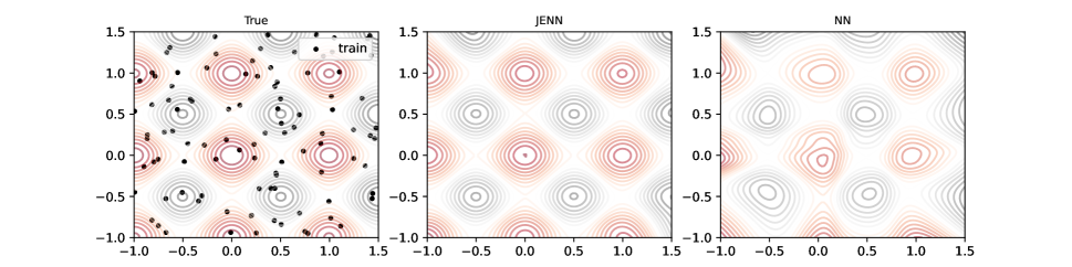
(d) $y=\sum_{i=1}^{2}\left(x_{i}^{2}-10\cos(2\pi x_{i})+10\right)$

Figure 2: Validation results

The theory developed in the previous section was implemented into an installable Python library for which a link was provided earlier. This section shows validation results for selected test functions in Fig. 2, where training data is shown as dots. These validation results compare JENN against a standard Neural Net (NN), defined as the equivalent neural network without gradient-enhancement.

All else being equal, it can clearly be seen that JENN outperforms NN in all cases, re-affirming the general concensus that gradient-enhancement achieves better accuracy with less data, so long as the computational cost of obtaining the Jacobian is not prohibitive in the first place. In Figs. 2a and 2b, where there are only three and four training samples respectively, NN fails to even capture the correct trend whereas JENN predicts the response almost perfectly. In Fig. 2d, where there are 100 samples, NN correctly captures the trend but contour lines are distorted, implying more samples would be needed to improve prediction. By contrast, under the same conditions, JENN predicts the Rastrigin function [25] almost perfectly.

Finally, it was also verified that runtime scales as $\mathcal{O}(n)$, as shown in Fig. 2c. This plot was obtained using the Rastrigin function to generate progressively larger datasets, train a new model, and record runtime on a MacBook Pro (2021).

V Example Application: Surrogate-Based Optimization

Surrogate-based optimization is the process of using a fast-running approximation, such as a neural networks, to optimize some slow-running function of interest, rather than directly using the function itself. This use-case typically arises when the response of interest takes too long to evaluate relative to the time scale of the application. For example, in real-time optimal control, one may wish to consider a neural network to make quick predictions of complicated physics when updating the trajectory[26]. The purpose of this section is to quantify the benefit of JENN relative to regular neural networks for gradient-based optimization. This will be accomplished by solving the following optimization problem:

Minimize: $$\quad\hat{y}=f(x_{1},x_{2})$$ (21)

With Respect To: $$\quad x_{1}\in\mathbb{R},x_{2}\in\mathbb{R}$$ (22)

Subject To: $$\quad-2\leq x_{1}\leq 2$$ (23)

$$\quad-2\leq x_{2}\leq 2$$ (24)

where $\hat{y}$ is a surrogate-model approximation to the Rosenbrock [27] function, which is used as an optimization benchmark because it exhibits a shallow valley with near-zero slope, which creates a significant challenge for surrogate-based optimization:

$$y=(1-x_{1})^{2}+100(x_{2}-x_{1}^{2})^{2}$$ (25)

Results are shown in Fig.3b, where optimization histories are shown for the true response and three surrogate-model approximations: NN, JENN, and JENN (polished). Training data is not shown to avoid clutter, but was generated by sampling the true response on a $9\times 9$ regular grid plus 100 latin hypercube points. The neural network training histories are also included in Fig. 3a, in order to verify that both neural networks converged to the same degree.

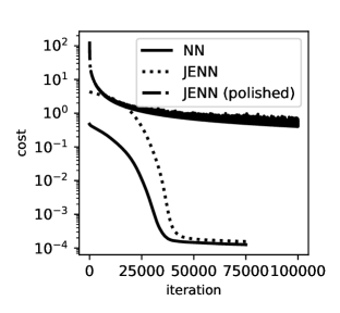
(a) Training history

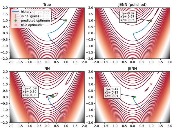
(b) Optimization history

Figure 3: Surrogate-based optimization results

V-A Results Without Polishing

Under perfect conditions, one would expect the optimization history to follow the same path for all models, but this is not observed: neither JENN nor NN reach the true location of this optimum situated at $(1,1)$. Carefully studying the contour lines of NN in the region where the Rosenbrock function flattens out, one can observe subtle undulations, within the noise of surrogate prediction error, which create artificial local minima that trap the optimizer. These effects are less pronounced for JENN, but the optimizer gets trapped nonetheless.

In hindsight, this finding is not surprising because neural networks learn by minimizing prediction error (recall Eq. III-D). Hence, by construction, there is more reward during training for accurately predicting regions of large change, where prediction error implies a large penalty, than there is for accurately predicting flat regions in the vicinity of a zero optimum, where prediction error penalties are negligible. This situation is at odds with the needs of gradient-based optimization which requires extreme accuracy near the optimum; accuracy elsewhere is desirable but less critical, provided slopes correctly point in the direction of improvement.

For a broad set of engineering problems, the results attained by these baseline models may be sufficiently accurate. However, there are situations where optimization accuracy is desirable if not critical, such as airfoil design where it is imperative that the final airfoil is free of undulations and non-smooth contours. An imperative research question therefore arises: how can these competing needs be reconciled?

V-B Results With Polishing

This situation can be ameliorated through “polishing.” Given a trained model, this approach consists of train it further after magnifying regions of interest. This is accomplished by judiciously setting $\gamma$ to prioritize specific training points belonging to that subspace. For example, flat regions could be magnified by allocating more importance to small slopes during training, using a radial basis functions centered on $\partial y/\partial x=0$ such as:

$$\gamma^{(t)}=1+\eta\cdot e^{-\left(\epsilon\frac{\partial y_{k}}{\partial x_{j}}^{(t)}\right)^{2}}~{}\forall~{}t,k,j$$ (26)

where $\eta$ and $\epsilon$ are hyperparameters that control the radius of influence of a point. They were set to $\eta=1000$ and $\epsilon=0.1$ in the results shown. Far away from any point $x^{(t)}$ where $\partial y/\partial x^{(t)}=0$, the weights are $\gamma^{(t)}\approx 1$ whereas near those points $\gamma^{(t)}\approx 1001$. This has the desired effect of disproportionately emphasizing regions of small slope ${\partial y_{k}}/{\partial x_{j}}$ during training by up to a factor of 1000 at the expense of de-emphasizing other regions, which is why it is necessary to start from an already trained model.

Final results are shown in Fig. 3b for the Rosenbrock test case, where it can be seen that JENN (polished) now recovers the true optimum almost exactly. Overall, this section demonstrates that jacobian-enhancement offer a quantifiable benefit over standard neural nets for SBO applications.

VI Noisy Partials

We now consider the effect of noisy partials. As mentioned in the introduction, many practical design applications rely on legacy software suites, such as missile DATCOM [28] during early design phases, for which analytical or automatically differentiated partials are not available. In this case, the only recourse for computing derivatives is finite difference. However, despite their attractive simplicity, it has been shown that finite difference methods are not as accurate as their counterparts [29]. It is therefore natural to wonder: how accurate must partials be in order to take advantage of JENN in design applications where finite difference is unavoidable?

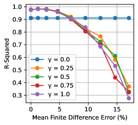
Figure 4: Predictive quality as a function of noisy partials

The answer to this question is shown by example in Fig. 4 using the Rastrigin function as a testbed once again, where $\gamma=0$ corresponds to baseline results for a standard neural network (gradient-enhancement off). Training data partial derivatives were obtained using finite difference with progressively increasing steps sizes. The corresponding mean finite difference error shown was computed against true analytical partials. It can clearly be seen that beyond seven percent error, the benefit of gradient-enhancement vanishes. In fact, beyond that threshold, partials are too inaccurate to provide useful information: accounting for erroneous partials is worse than not accounting for partials at all. These results are welcome, as they demonstrate that the usefulness of gradient-enhanced methods is not restricted to perfectly accurate partials; even noisy partials can be useful (within a reasonable threshold).

Finally, these results further show that there is no benefit to setting $\gamma$ to values other than zero or one; it does not mitigate the effect of noisy partials. For most applications, the hyperparameter $\gamma$ should therefore be treated as a binary scalar to turn gradient-enhancement on ($\gamma=1$) or off ($\gamma=0$); except in special situations which call for distribution (rather than a scalar) such as polishing, as previously illustrated, or incomplete partials. The latter is likely to be a common scenario where partials are not available for all inputs, in which case $\gamma$ can be used to turn gradient-enhancement on/off depending on whether a partial is missing or not (i.e. resulting in a tensor of zeros and ones).

VII Conclusion

In summary, this research developed a jacobian-enhanced, deep-learning formulation for dense multi-layer perceptrons and successfully validated the implementation against selected canonical test functions. It was shown that validation results support the general consensus that gradient-enhanced methods require less training data and achieve better accuracy than their non-gradient-enhanced counterparts, provided the cost of obtaining training data partials is not prohibitive in the first place. It was further shown that JENN outperforms standard neural networks in the context of surrogate-based optimization. However, it was observed that a learning procedure which minimizes any version of the least squares estimator is at odds with the needs of gradient descent in the vicinity of the optimum, where slopes are close to zero. It was further shown that this shortcoming can be overcome through polishing, which can be used to prioritize salient regions of interest through judicious use of hyperparameters. This unique feature enabled by the present formulation provides an additional knob for tuning optimized solution accuracy in situations that call for it. The ideas and findings of this paper have been published as an open-source library to allow readers to validate the results, and hopefully assist them in their surrogate modeling efforts.

VIII Key Equations in Vectorized Form

This section provides vectorized equations to facilitate re-implementation or as a companion guide to the JENN library.

VIII-A Data Structures

Using capital letters, notation can be extended to matrix notation to account for all $m$ training examples, starting with training data inputs and outputs:

$$\boldsymbol{X} =\left[\begin{matrix}x_{1}^{(1)}&\dots&x_{1}^{(m)}\\ \vdots&\ddots&\vdots\\ x_{n_{x}}^{(1)}&\dots&x_{n_{x}}^{(m)}\\ \end{matrix}\right]\in\mathbb{R}^{n_{x}\times m}$$ (27)

$$\boldsymbol{Y} =\left[\begin{matrix}y_{1}^{(1)}&\dots&y_{1}^{(m)}\\ \vdots&\ddots&\vdots\\ y_{n_{y}}^{(1)}&\dots&y_{n_{y}}^{(m)}\\ \end{matrix}\right]\in\mathbb{R}^{n_{y}\times m}$$ (28)

The associated Jacobians are formatted as:

$$\boldsymbol{J}=\left[\begin{matrix}{\left[\begin{matrix}\dfrac{\partial y_{1}}{\partial x_{1}}^{(1)}&\dots&\dfrac{\partial y_{1}}{\partial x_{1}}^{(m)}\\ \vdots&\ddots&\vdots\\ \dfrac{\partial y_{1}}{\partial x_{n_{x}}}^{(1)}&\dots&\dfrac{\partial y_{1}}{\partial x_{n_{x}}}^{(m)}\\ \end{matrix}\right]}\\ \vdots\\ {\left[\begin{matrix}\dfrac{\partial y_{n_{y}}}{\partial x_{1}}^{(1)}&\dots&\dfrac{\partial y_{n_{y}}}{\partial x_{1}}^{(m)}\\ \vdots&\ddots&\vdots\\ \dfrac{\partial y_{n_{y}}}{\partial x_{n_{x}}}^{(1)}&\dots&\dfrac{\partial y_{n_{y}}}{\partial x_{n_{x}}}^{(m)}\\ \end{matrix}\right]}\end{matrix}\right]\in\mathbb{R}^{n_{y}\times n_{x}\times m}$$ (29)

Note that the hyperparameters $\beta,\gamma$ can either be scalars or real arrays of the same shape as ${\bf Y}$ and ${\bf J}$, respectively. The shape of the neural network parameters to be learned (i.e. weights and biases) is independent of the number of training examples. They depend only on layer sizes and are denoted as:

$${\bf W}^{[l]} =\left[\begin{matrix}w_{11}^{[l]}&\dots&w_{1n^{[l-1]}}^{[l]}\\ \vdots&\ddots&\vdots\\ w_{n^{[l]}1}^{[l]}&\dots&w_{n^{[l]}n^{[l-1]}}^{[l]}\end{matrix}\right]~{}\in\mathbb{R}^{n^{[l]}\times n^{[l-1]}}$$ (30)

$$\boldsymbol{b}^{[l]} =\left[\begin{matrix}b_{1}^{[l]}\\ \vdots\\ b_{n^{[l]}}^{[l]}\end{matrix}\right]~{}\in\mathbb{R}^{n^{[l]}\times 1}\quad\forall\quad 1<l\leq L$$ (31)

However, hidden layer activations do depend on the number of examples and are stored as:

$${\bf A}^{[l]} =\left[\begin{matrix}a_{1}^{(1)}&\dots&a_{1}^{(m)~{}}\\ \vdots&\ddots&\vdots\\ a_{n^{[l]}}^{(1)}&\dots&a_{n^{[l]}}^{(m)~{}}\end{matrix}\right]~{}\in\mathbb{R}^{n^{[l]}\times m}$$ (32)

$${\bf Z}^{[l]} =\left[\begin{matrix}z_{1}^{(1)}&\dots&z_{1}^{(m)~{}}\\ \vdots&\ddots&\vdots\\ z_{n^{[l]}}^{(1)}&\dots&z_{n^{[l]}}^{(m)~{}}\end{matrix}\right]~{}\in\mathbb{R}^{n^{[l]}\times m}$$ (33)

The associated hidden layer derivatives w.r.t. inputs are stored as:

$${\bf A}^{\prime[l]} =\left[\begin{matrix}{\left[\begin{matrix}\dfrac{\partial a_{1}}{\partial x_{1}}^{(1)}&\dots&\dfrac{\partial a_{1}}{\partial x_{1}}^{(m)}\\ \vdots&\ddots&\vdots\\ \dfrac{\partial a_{1}}{\partial x_{n_{x}}}^{(1)}&\dots&\dfrac{\partial a_{1}}{\partial x_{n_{x}}}^{(m)}\\ \end{matrix}\right]}\\ \vdots\\ {\left[\begin{matrix}\dfrac{\partial a_{n^{[l]}}}{\partial x_{1}}^{(1)}&\dots&\dfrac{\partial a_{n^{[l]}}}{\partial x_{1}}^{(m)}\\ \vdots&\ddots&\vdots\\ \dfrac{\partial a_{n^{[l]}}}{\partial x_{n_{x}}}^{(1)}&\dots&\dfrac{\partial a_{n^{[l]}}}{\partial x_{n_{x}}}^{(m)}\\ \end{matrix}\right]}\end{matrix}\right]\in\mathbb{R}^{n^{[l]}\times n_{x}\times m}$$ (34)

$${\bf Z}^{\prime[l]} =\left[\begin{matrix}{\left[\begin{matrix}\dfrac{\partial z_{1}}{\partial x_{1}}^{(1)}&\dots&\dfrac{\partial z_{1}}{\partial x_{1}}^{(m)}\\ \vdots&\ddots&\vdots\\ \dfrac{\partial z_{1}}{\partial x_{n_{x}}}^{(1)}&\dots&\dfrac{\partial z_{1}}{\partial x_{n_{x}}}^{(m)}\\ \end{matrix}\right]}\\ \vdots\\ {\left[\begin{matrix}\dfrac{\partial z_{n^{[l]}}}{\partial x_{1}}^{(1)}&\dots&\dfrac{\partial z_{n^{[l]}}}{\partial x_{1}}^{(m)}\\ \vdots&\ddots&\vdots\\ \dfrac{\partial z_{n^{[l]}}}{\partial x_{n_{x}}}^{(1)}&\dots&\dfrac{\partial z_{n^{[l]}}}{\partial x_{n_{x}}}^{(m)}\\ \end{matrix}\right]}\end{matrix}\right]\in\mathbb{R}^{n^{[l]}\times n_{x}\times m}$$ (35)

It follows that hidden layer derivatives w.r.t. a specific input $x_{j}$ are formatted as:

$${\bf A}_{j}^{\prime[l]} =\left[\begin{matrix}\dfrac{\partial a_{1}}{\partial x_{j}}^{(1)}&\dots&\dfrac{\partial a_{1}}{\partial x_{j}}^{(m)}\\ \vdots&\ddots&\vdots\\ \dfrac{\partial a_{n^{[l]}}}{\partial x_{j}}^{(1)}&\dots&\dfrac{\partial a_{n^{[l]}}}{\partial x_{j}}^{(m)}\\ \end{matrix}\right]~{}\in\mathbb{R}^{n^{[l]}\times m}$$ (36)

$${\bf Z}_{j}^{\prime[l]} =\left[\begin{matrix}\dfrac{\partial z_{1}}{\partial x_{j}}^{(1)}&\dots&\dfrac{\partial z_{1}}{\partial x_{j}}^{(m)}\\ \vdots&\ddots&\vdots\\ \dfrac{\partial z_{n^{[l]}}}{\partial x_{j}}^{(1)}&\dots&\dfrac{\partial z_{n^{[l]}}}{\partial x_{j}}^{(m)}\\ \end{matrix}\right]~{}\in\mathbb{R}^{n^{[l]}\times m}$$ (37)

Finally, the back propagation derivatives w.r.t. parameters are:

$$\dfrac{\partial\mathcal{J}}{\partial{\bf W}^{[l]}} =\left[\begin{matrix}\dfrac{\partial\mathcal{J}}{\partial w_{11}}&\dots&\dfrac{\partial\mathcal{J}}{\partial w_{1n^{[l-1]}}}\\ \vdots&\vdots&\vdots\\ \dfrac{\partial\mathcal{J}}{\partial w_{n^{[l]}1}}&\dots&\dfrac{\partial\mathcal{J}}{\partial w_{n^{[l]}n^{[l-1]}}}\end{matrix}\right]~{}\in\mathbb{R}^{n^{[l]}\times n^{[l-1]}}$$ (38a)

$$\dfrac{\partial\mathcal{J}}{\partial\boldsymbol{b}^{[l]}} =\left[\begin{matrix}\dfrac{\partial\mathcal{J}}{\partial b_{1}}\\ \vdots\\ \dfrac{\partial\mathcal{J}}{\partial b_{n^{[l]}}}\end{matrix}\right]~{}\in\mathbb{R}^{n^{[l]}\times 1}\quad\forall\quad l\in(1,L]$$ (38b)

VIII-B Forward Propagation (Eq. 3)

$${\bf Z}^{[l]} ={\bf W}^{[l]}\odot{\bf A}^{[l-1]}+\boldsymbol{b}^{[l]} \quad\forall~{}1<l\leq L$$ (39a)

$${\bf Z}^{{}^{\prime}[l]} ={\bf W}^{[l]}\odot{\bf A}_{j}^{{}^{\prime}[l-1]}+\boldsymbol{b}^{[l]} \quad\forall~{}1\leq j\leq n_{x}$$ (39b)

$${\bf A}^{[l]} =g\left({\bf Z}^{[l]}\right) \quad\forall~{}1<l\leq L$$ (40a)

$${\bf A}_{j}^{{}^{\prime}[l]} =g\left({\bf Z}^{[l]}\right)\odot{\bf Z}_{j}^{{}^{\prime}[l]} \quad\forall~{}1\leq j\leq n_{x}$$ (40b)

VIII-C Parameter Update (Eq. 8)

$${\bf W}^{[l]} :={\bf W}^{[l]}-\alpha\frac{\partial\mathcal{J}}{\partial{\bf W}^{[l]}}$$ (41a)

$$\boldsymbol{b}^{[l]} :=\boldsymbol{b}^{[l]}-\alpha\frac{\partial\mathcal{J}}{\partial\boldsymbol{b}^{[l]}} \quad\forall~{}1<l\leq L$$ (41b)

VIII-D Backward Propagation (Eqs. 15–16, 17, 20)

The loss function partials w.r.t. last layer activations are:

$$\frac{\partial\mathcal{L}}{\partial{\bf A}^{[L]}} =\beta\odot\left({\bf A}^{[L]}-{\bf Y}\right)$$ (42a)

$$\frac{\partial\mathcal{L}}{\partial{\bf A}^{\prime[L]}} =\gamma\odot\left({\bf A}^{\prime[L]}-{\bf Y^{\prime}}\right)$$ (42b)

The loss function partials w.r.t. hidden layer activations are:

$$\frac{\partial\mathcal{L}}{\partial{\bf A}^{[l-1]}} ={\bf W}^{\top[l]}\cdot\left(g^{\prime}\left({\bf Z}^{[l]}\right)\odot\frac{\partial\mathcal{L}}{\partial{\bf A}^{[l]}}\right)\dots$$ (43a)

$$\dots +\sum_{j=1}^{n_{x}}{\bf W}^{\top[l]}\cdot\left(g^{\prime\prime}\left({\bf Z}^{[l]}\right)\odot{\bf Z}_{j}^{\prime[l]}\odot\frac{\partial\mathcal{L}}{\partial{\bf A}_{j}^{\prime[l]}}\right)$$

$$\frac{\partial\mathcal{L}}{\partial{\bf A_{j}}^{\prime[l-1]}} =\sum_{j=1}^{n_{x}}{\bf W}^{\top[l]}\cdot\left(g^{\prime}\left({\bf Z}^{[l]}\right)\odot\frac{\partial\mathcal{L}}{\partial{\bf A}_{j}^{\prime[l]}}\right)$$ (43b)

The loss function partials w.r.t. neural net parameters are:

$$\frac{\partial\mathcal{L}}{\partial{\bf W}^{[l]}} =\frac{\partial\mathcal{L}}{\partial{\bf A}^{[l]}}\odot g^{\prime}\left({\bf Z}^{[l]}\right)\odot{\bf A}^{[l-1]}+\sum_{j=1}^{n_{x}}\frac{\partial\mathcal{L}}{\partial{\bf A}_{j}^{\prime[l]}}\odot\bigg{[}\dots$$

$$\dots g^{\prime\prime}\left({\bf Z}^{[l]}\right)\odot{\bf Z}_{j}^{\prime[l]}\odot{\bf A}^{\prime[l-1]}+g^{\prime}\left({\bf Z}^{[l]}\right){\bf A}_{j}^{\prime[l-1]}\bigg{]}$$ (44a)

$$\frac{\partial\mathcal{L}}{\partial{\bf b}_{[l]}} =\frac{\partial\mathcal{L}}{\partial{\bf A}^{[l]}}\odot g^{\prime}\left({\bf Z}^{[l]}\right)+\sum_{j=1}^{n_{x}}\frac{\partial\mathcal{L}}{\partial{\bf A}_{j}^{\prime[l]}}\odot g^{\prime\prime}\left({\bf Z}^{[l]}\right)\odot{\bf Z}_{j}^{\prime[l]}$$ (44b)

Finally, the cost function partials w.r.t. neural net parameters are:

$$\frac{\partial\mathcal{J}}{\partial{\bf W}^{[l]}} =\frac{1}{m}S\left(\frac{\partial\mathcal{L}}{\partial{\bf W}^{[l]}}\right)+\frac{\lambda}{m}{\bf W}^{[l]}$$ (45a)

$$\frac{\partial\mathcal{J}}{\partial\boldsymbol{b}^{[l]}} =\frac{1}{m}S\left(\frac{\partial\mathcal{L}}{\partial{\bf W}^{[l]}}\right)$$ (45b)

where S is used to denote the vectorized summation along the last axis of an array. Any other summation shown above implies that it could not be vectorized and required a loop. This only happened when summing over partials. Hence, the number of loops needed equals the number of inputs $n_{x}$, which is usually negligible compared to the size of the training data $m$. The latter is the critical dimension to be vectorized.

References

- [1] A. J. Keane and P. B. Nair, “Computational Approaches for Aerospace Design Computational.” John Wiley & Sons Ltd, The Atrium, Southern Gate, Chichester, West Sussex PO19 8SQ, England: Wiley, 2005, ch. 5, 7, pp. 211–270, 301–326.
- [2] A. I. J. Forrester, A. Sobester, and A. J. Keane, Engineering Design via Surrogate Modelling - A Practical Guide. Wiley, 2008.
- [3] E. Iuliano, Adaptive Sampling Strategies for Surrogate-Based Aerodynamic Optimization. Cham: Springer International Publishing, 2016, pp. 25–46. [Online]. Available: https://doi.org/10.1007/978-3-319-21506-8_2
- [4] J. R. R. A. Martins and A. Ning, Engineering Design Optimization. Cambridge University Press, 2021, ch. 10, pp. 373–422.
- [5] N. V. Queipo, R. T. Haftka, W. Shyy, T. Goel, R. Vaidyanathan, and P. K. Tucher, “Surrogate-based analysis and optimization,” Progress in Aerospace Sciences, vol. 41, pp. 1–28, 2005.
- [6] A. Haridy, “Review on surrogate-based global optimization with biomedical applications,” Biomedical Journal of Scientific & Technical Research, vol. 53, no. 3, pp. 44 786–44 792, 2023.
- [7] L. Bliek, “A survey on sustainable surrogate-based optimisation,” Sustainability, vol. 14, no. 7, 2022. [Online]. Available: https://www.mdpi.com/2071-1050/14/7/3867
- [8] Review of Metamodeling Techniques in Support of Engineering Design Optimization, ser. International Design Engineering Technical Conferences and Computers and Information in Engineering Conference, vol. Volume 1: 32nd Design Automation Conference, Parts A and B, 09 2006. [Online]. Available: https://doi.org/10.1115/DETC2006-99412
- [9] T. D. Robinson, M. S. Eldred, K. E. Willcox, and R. Haimes, “Surrogate-based optimization using multifidelity models with variable parameterization and corrected space mapping,” AIAA Journal, vol. 46, no. 11, pp. 2814–2822, 2008. [Online]. Available: https://doi.org/10.2514/1.36043
- [10] K. Giannakoglou, D. Papadimitriou, and I. Kampolis, “Aerodynamic shape design using evolutionary algorithms and new gradient-assisted metamodels,” Computer Methods in Applied Mechanics and Engineering, vol. 195, no. 44, pp. 6312–6329, 2006. [Online]. Available: https://www.sciencedirect.com/science/article/pii/S0045782506000338
- [11] M. A. Bouhlel, S. He, and J. R. R. A. Martins, “Scalable gradient–enhanced artificial neural networks for airfoil shape design in the subsonic and transonic regimes,” Structural and Multidisciplinary Optimization, vol. 61, no. 4, pp. 1363–1376, 2020. [Online]. Available: https://doi.org/10.1007/s00158-020-02488-5
- [12] J. R. Nagawkar, L. T. Leifsson, and P. He, Aerodynamic Shape Optimization Using Gradient-Enhanced Multifidelity Neural Networks. [Online]. Available: https://arc.aiaa.org/doi/abs/10.2514/6.2022-2350
- [13] A. Jameson, “Aerodynamic design via control theory,” Journal of Scientific Computing, vol. 3, no. 3, pp. 233–260, 1988. [Online]. Available: https://doi.org/10.1007/BF01061285
- [14] M. Abadi, A. Agarwal, P. Barham, E. Brevdo, Z. Chen, C. Citro, G. S. Corrado, A. Davis, J. Dean, M. Devin, S. Ghemawat, I. Goodfellow, A. Harp, G. Irving, M. Isard, Y. Jia, R. Jozefowicz, L. Kaiser, M. Kudlur, J. Levenberg, D. Mané, R. Monga, S. Moore, D. Murray, C. Olah, M. Schuster, J. Shlens, B. Steiner, I. Sutskever, K. Talwar, P. Tucker, V. Vanhoucke, V. Vasudevan, F. Viégas, O. Vinyals, P. Warden, M. Wattenberg, M. Wicke, Y. Yu, and X. Zheng, “TensorFlow: Large-scale machine learning on heterogeneous systems,” 2015, software available from tensorflow.org. [Online]. Available: https://www.tensorflow.org/
- [15] A. Paszke, S. Gross, F. Massa, A. Lerer, J. Bradbury, G. Chanan, T. Killeen, Z. Lin, N. Gimelshein, L. Antiga, A. Desmaison, A. Köpf, E. Yang, Z. DeVito, M. Raison, A. Tejani, S. Chilamkurthy, B. Steiner, L. Fang, J. Bai, and S. Chintala, PyTorch: an imperative style, high-performance deep learning library. Red Hook, NY, USA: Curran Associates Inc., 2019.
- [16] F. Pedregosa, G. Varoquaux, A. Gramfort, V. Michel, B. Thirion, O. Grisel, M. Blondel, P. Prettenhofer, R. Weiss, V. Dubourg, J. Vanderplas, A. Passos, D. Cournapeau, M. Brucher, M. Perrot, and E. Duchesnay, “Scikit-learn: Machine learning in Python,” Journal of Machine Learning Research, vol. 12, pp. 2825–2830, 2011.
- [17] P. Saves, R. Lafage, N. Bartoli, Y. Diouane, J. Bussemaker, T. Lefebvre, J. T. Hwang, J. Morlier, and J. R. R. A. Martins, “SMT 2.0: A surrogate modeling toolbox with a focus on hierarchical and mixed variables gaussian processes,” Advances in Engineering Sofware, vol. 188, p. 103571, 2024.
- [18] L. Laurent, R. Le Riche, B. Soulier, and P.-A. Boucard, “An overview of gradient-enhanced metamodels with applications,” Archives of Computational Methods in Engineering, vol. 26, no. 1, pp. 61–106, 2019. [Online]. Available: https://doi.org/10.1007/s11831-017-9226-3
- [19] R. Sellar and S. Batill, Concurrent Subspace Optimization using gradient-enhanced neural network approximations. [Online]. Available: https://arc.aiaa.org/doi/abs/10.2514/6.1996-4019
- [20] W. Liu and S. Batill, Gradient-enhanced neural network response surface approximations. [Online]. Available: https://arc.aiaa.org/doi/abs/10.2514/6.2000-4923
- [21] J. Hoffman, D. A. Roberts, and S. Yaida, “Robust learning with jacobian regularization,” 2019.
- [22] J. Yu, L. Lu, X. Meng, and G. E. Karniadakis, “Gradient-enhanced physics-informed neural networks for forward and inverse pde problems,” Computer Methods in Applied Mechanics and Engineering, vol. 393, p. 114823, 2022. [Online]. Available: https://www.sciencedirect.com/science/article/pii/S0045782522001438
- [23] A. Ng, “Deep learning specialization: Neural networks and deep learning,” https://www.coursera.org/specializations/deep-learning, 2017, accessed October 2017.
- [24] D. P. Kingma and J. Ba, “Adam: A method for stochastic optimization,” 2017.
- [25] L. A. Rastrigin, “Systems of extremal control,” Nauka, 1974.
- [26] C. Sánchez-Sánchez and D. Izzo, “Real-time optimal control via deep neural networks: Study on landing problems,” Journal of Guidance, Control, and Dynamics, vol. 41, no. 5, pp. 1122–1135, 2018. [Online]. Available: https://doi.org/10.2514/1.G002357
- [27] H. H. Rosenbrock, “An Automatic Method for Finding the Greatest or Least Value of a Function,” The Computer Journal, vol. 3, no. 3, pp. 175–184, 01 1960. [Online]. Available: https://doi.org/10.1093/comjnl/3.3.175
- [28] C. Rosema, J. Doyle, and W. B. Blake, “Missile data compendium (datcom): user manual,” 2014, Air Force Research Laboratories, Technical Report AFRL-RQ-WP-TR-2014-0281.
- [29] J. R. R. A. Martins and J. T. Hwang, “Review and unification of methods for computing derivatives of multidisciplinary computational models,” AIAA Journal, vol. 51, no. 11, pp. 2582–2599, 2013. [Online]. Available: https://doi.org/10.2514/1.J052184