Distribution of Hooks in Self-Conjugate Partitions

Abstract.

We confirm the speculation that the distribution of $t$-hooks among unrestricted integer partitions essentially descends to self-conjugate partitions. Namely, we prove that the number of hooks of length $t$ among the size $n$ self-conjugate partitions is asymptotically normally distributed with mean $\mu_{t}(n)$ and variance $\sigma_{t}(n)^{2}$

$$\mu_{t}(n)\sim\frac{\sqrt{6n}}{\pi}+\frac{3}{\pi^{2}}-\frac{t}{2}\ \ \ {\text{\rm and}}\ \ \ \sigma_{t}^{2}(n)\sim\frac{\left(\pi^{2}-6\right)\sqrt{6n}}{\pi^{3}}.$$

1. Introduction and Statement of results

A partition of a non-negative integer $n$ is a non-increasing sequence of positive integers $\left(\lambda_{1},\dots,\lambda_{\ell}\right)$ whose terms sum to $n$. We write $\lambda\vdash n$ to denote that $\lambda$ is a partition of $n$. Partitions play an important role in many areas of mathematics, including combinatorics, geometry, mathematical physics, number theory and representation theory. Here we study the combinatorial statistics of partition hook numbers.

For a partition $\lambda$, integers $j,k\geq 1$ and any cell $\left(j,k\right)$ in the Young diagram of $\lambda$, the corresponding hook number $h(j,k)$ is the length of the hook $H(j,k)$ formed with the cell $\left(j,k\right)$ as its upper corner. In terms of the conjugate partition $\lambda^{\prime}=\left(\lambda_{1}^{\prime},\dots,\lambda_{r}^{\prime}\right)$, we may write $h(j,k)=\left(\lambda_{j}-j\right)+\left(\lambda_{k}^{\prime}-k\right)+1$. Below, we see an example demonstrating the computation of hook numbers.

$$\ytableau 7&6431\\ 5421\\ 21$$

Figure 1. Hook numbers for the partition $\lambda=\left(5,4,2\right)$.

Hook numbers play a significant role in the representation theory of the symmetric group, where the partitions of $n$ capture the irreducible representations of $S_{n}.$ Indeed, if $\mathcal{H}(\lambda)$ is the multiset of hook lengths in $\lambda$ and $\rho_{\lambda}$ is the irreducible representation of $S_{n}$ associated with $\lambda$, then the Frame–Thrall–Robinson hook length formula gives the dimension

$$\mathrm{dim}\left(\rho_{\lambda}\right)=\dfrac{n!}{\prod_{h\in\mathcal{H}(\lambda)}h}.$$

Furthermore, hook numbers are prominent in mathematical physics and number theory, For example, we highlight the work of Nekrasov and Okounkov [13] and Westbury [16], who recognized the deep properties of hook numbers through their extraordinary $q$-series identity

$$\sum_{\lambda}q^{|\lambda|}\prod_{h\in\mathcal{H}(\lambda)}\left(1-\dfrac{z}{h^{2}}\right)=\prod_{n\geq 1}\left(1-q^{n}\right)^{z-1}.$$ (1.1)

Using this formula and its generalizations due to Han [12], many connections have been drawn between hook numbers and modular forms, which have led to many interesting results, including theorems about cranks for Ramanujan’s partition congruences [9] and class numbers of imaginary quadratic fields [15].

Establishing combinatorial statistics for partitions is an important and growing field in partition theory (see for instance [2, 4, 6, 10, 11]). Here we consider the statistics of hook numbers. Recently, Griffin, Tsai and the second author [10] studied the counting function

$$N_{t}(\lambda):=\#\{h\in\mathcal{H}(\lambda):h=t\}.$$

If we let $N_{t}(n)$ be the random variable which takes the value $N_{t}(\lambda)$ for $\lambda$ a random partition of $n$, then [10] proved the following theorem.

Theorem 1.1 ([10, Theorem 1.1]).

For $t\geq 1$ an integer, the function $N_{t}(n)$ has an asymptotically normal distribution as $n\to\infty$ with mean asymptotic to $\frac{\sqrt{6n}}{\pi}-\frac{t}{2}$ and variance asymptotic to $\frac{\left(\pi^{2}-6\right)\sqrt{6n}}{2\pi^{3}}$.

It is natural to ask whether the same phenomenon holds for the restricted partition families. In this paper, we show that this is essentially the case for self-conjugate partitions. To make this precise, for integers $t\geq 1$ we study the arithmetic statistics of $N_{t}(\lambda)$ considered as a random variable restricted to the class $\mathcal{SC}$ of self-conjugate partitions. Such a study requires the two-variable generating function which simultaneously tracks the size and hook counts of self-conjugate partitions; that is, we require an explicit formula for

$$F_{t}(T;q):=\sum_{\lambda\in{\mathcal{S}C}}T^{N_{t}(\lambda)}q^{|\lambda|}=:\sum_{n\geq 0}\mathrm{sc}_{t}(n;T)q^{n}.$$ (1.2)

By means of the Littlewood bijection for $t$-core partitions, Amdeberhan, Andrews and two of the authors [1] derived such a formula in order to address conjectures of the first author and collaborators [3, 7] on the arithmetic of hook counts in self-conjugate partitions. In this way we obtain the following direct analog of Theorem 1.1.

Theorem 1.2.

Let $t\geq 1$ be an integer, and consider the random variable $\widehat{N}_{t}(n)$ giving the distribution of $N_{t}$ on the set ${\mathcal{S}C}(n)$ of self-conjugate partitions of $n$. Then as $n\to\infty$, $\widehat{N}_{t}(n)$ is asymptotically normally distributed with mean $\mu_{t}(n)\sim\frac{\sqrt{6n}}{\pi}-\frac{t}{2}+\frac{3}{\pi^{2}}$ and variance $\sigma_{t}(n)^{2}\sim\frac{(\pi^{2}-6)\sqrt{6n}}{\pi^{3}}+\frac{3t}{\pi^{2}}-\frac{t^{2}}{4}-\frac{279}{16\pi^{4}}$.

Remark 1.3.

It is interesting to note that, in comparison to Theorem 1.1, the main term of the mean is the same, but the main term of the variance is doubled in the self-conjugate case.

Example 1.4.

In the case of $t=2$, Theorem 1.2 says that as $n\to\infty$ the number of 2-hooks in a random self-conjugate partition is asymptotically normal with mean $\mu_{2}(n)\sim\frac{\sqrt{6n}}{\pi}-1+\frac{3}{\pi^{2}}$ and variance $\sigma_{2}(n)^{2}\sim\frac{(\pi^{2}-6)\sqrt{6n}}{\pi^{3}}+\frac{3}{\pi^{2}}-1+\frac{279}{16\pi^{4}}$. The convergence of this distribution in the case $t=2$ is demonstrated below.

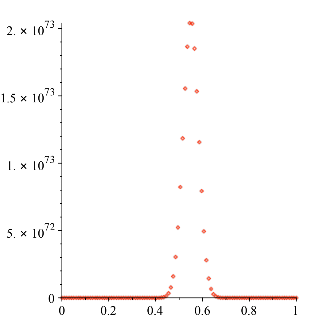
Figure 2. Renormalized plot of the coefficients of $\mathrm{sc}_{2}(5000;T)$.

Table 1 shows the convergence of the measured means $\mu_{2}(n)$ to the asymptotic $\mu(n):=\frac{\sqrt{6n}}{\pi}$:

$n$	$\mu_{2}(n)$	$\mu(n)$	$\mu_{2}(n)/\mu(n)$
100	9.17483	7.79697	1.17672
500	18.76417	17.43455	1.07626
1000	25.97841	24.65618	1.05363
5000	56.44511	55.13289	1.0238

Table 1. Data showing the asymptotic $\mu_{2}(n)\sim\mu(n)$ as $n\to\infty$.

The paper is organized as follows. In Section 2 we collect preliminary definitions and asymptotic lemmas we will need, which will be derived from the Euler–Maclaurin summation formula. In Section 3 we apply various asymptotic lemmas and the saddle point method in order to obtain required asymptotics for the polynomials $\mathrm{sc}_{t}(n;T)$ for ranges of $T$ as $n\to\infty$. Finally, in Section 4 we filter these asymptotics through the method of moments in order to prove Theorem 1.2.

2. Nuts and Bolts

2.1. Generating functions

Here, we state the formula of [1] for the generating function $F_{t}(T;q)$. In order to state this formula, we need the notation

$$\left(a;q\right)_{n}:=\prod_{j=0}^{n-1}\left(1-aq^{j}\right),\ \ \ n\in\mathbb{N}_{0}\cup\{\infty\}.$$

With this notation, we state their result.

Theorem 2.1 ([1, Theorem 1.1]).

Let $t\geq 1$ be an integer. Then the following are true:

1. If $t$ is even, then we have

   $$F_{t}(T;q)=\left(-q;q^{2}\right)_{\infty}\cdot\left(\left(1-T^{2}\right)q^{2t};q^{2t}\right)_{\infty}^{\frac{t}{2}}.$$

2. If $t$ is odd, we have

   $$F_{t}(T;q)=\left(-q;q^{2}\right)_{\infty}\cdot H^{*}(T;q^{t})\cdot\left(\left(1-T^{2}\right)q^{2t};q^{2t}\right)_{\infty}^{\frac{t-1}{2}},$$

   where $H^{*}(T;q)$ is defined by

   $$H^{*}(T;q):=\dfrac{1}{2T}\left[C_{T}^{+}\left(\sqrt{1-T^{2}};-q\right)_{\infty}+C_{T}^{-}\left(-\sqrt{1-T^{2}};-q\right)_{\infty}\right],$$ (2.1)

   where for convenience we define the constants

   $$C_{T}^{\pm}:=1\pm\sqrt{\dfrac{1-T}{1+T}}.$$

We note that $H^{*}$ can also be represented in terms of $q$-hypergeometric series [1, Equation 3.1] as

$$H^{*}(T;q)=\left(1-\dfrac{1}{T}\right)\sum_{n\geq 0}\dfrac{(T^{2}-1)^{n}q^{2n^{2}+n}}{\left(q^{2};q^{2}\right)_{n}\left(-q;q^{2}\right)_{n+1}}+\dfrac{1}{T}\sum_{n\geq 0}\dfrac{(T^{2}-1)^{n}q^{2n^{2}-n}}{\left(q^{2};q^{2}\right)_{n}\left(-q;q^{2}\right)_{n}}.$$ (2.2)

We primarily use the representation in terms of products because it is more convenient for much of our asymptotic analysis, although there are certain kinds of calculations which are easier in the $q$-hypergeometric form.

2.2. The dilogarithm function

We recall the dilogarithm function $\mathrm{Li}_{2}\left(z\right)$, which is given by

$$\mathrm{Li}_{2}(z):=\sum_{k\geq 1}\dfrac{z^{k}}{k^{2}}$$

for $|z|<1$ and elsewhere by the standard analytic continuation having a branch cut on the line $(1,\infty)$. Dilogarithm functions appear frequently when computing asymptotic expansions of infinite products of the general shape $\left(a;q\right)_{\infty}$. For our calculations, we will need the elementary identity [18, pg. 9]

$$\mathrm{Li}_{2}\left(z\right)+\mathrm{Li}_{2}\left(-z\right)=\dfrac{\mathrm{Li}_{2}\left(z^{2}\right)}{2},$$ (2.3)

as well as the derivative [18, pg. 5]

$$\dfrac{d}{dz}\mathrm{Li}_{2}\left(z\right)=-\dfrac{\log(1-z)}{z}$$ (2.4)

and the so-called distribution property [18, pg. 9]

$$\mathrm{Li}_{2}\left(x\right)=n\sum_{z^{n}=x}\mathrm{Li}_{2}\left(z\right).$$ (2.5)

2.3. Euler–Maclaurin summation formulas

As infinite products are often unwieldy to deal with directly, a common technique when analyzing $\left(a;q\right)_{\infty}$ asymptotically is to first take a logarithm and subsequently use techniques for infinite sums. In particular, we will make use of an asymptotic variation of the Euler–Maclaurin summation formula [5, 17]. To state this result, we will say that a function $f(z)$ satisfies the asymptotic $f(z)\sim\sum_{n\geq n_{0}}c_{n}z^{n}$ as $z\to 0$ if $f(z)-\sum_{n=n_{0}}^{N-1+n_{0}}c_{n}z^{n}=O_{N}\left(z^{N}\right)$ for each $N\geq 1$.

Lemma 2.2 ([5, Theorem 1.2]).

Suppose that $0\leq\theta<\frac{\pi}{2}$ and let

$$D_{\theta}:=\{re^{i\alpha}:r\geq 0\mbox{ and }|\alpha|\leq\theta\}.$$

Suppose $f(z)$ is holomorphic in a domain containing $D_{\theta}$, and that $f$ and all its derivatives are of sufficient decay as $|z|\to\infty$ (i.e. decays at least as quickly as $|z|^{-1-\varepsilon}$ for some $\varepsilon>0$). Suppose also that $f$ has the asymptotic expansion $f(z)\sim\sum_{n\geq 0}c_{n}z^{n}$ near $z=0$. Then for any $0<a\leq 1$, we have as $z\to 0$ that

$$\sum_{m\geq 0}f\left((m+a)z\right)\sim\dfrac{1}{z}\int_{0}^{\infty}f(x)dx-\sum_{n\geq 0}c_{n}\dfrac{B_{n+1}(a)}{n+1}z^{n},$$

where $B_{n}(x)$ are the Bernoulli polynomials.

We will apply Euler–Maclaurin summation many times throughout the paper, and in particular we will be interested in using not only a function $f$ as above, but several of its derivatives as well. In order to do this most efficiently, we derive the following corollary.

Corollary 2.3.

Suppose that $0\leq\theta<\frac{\pi}{2}$ and let $f:{\mathbb{C}}\rightarrow{\mathbb{C}}$ be holomorphic in a domain containing $D_{\theta}$, so that in particular $f$ is holomorphic at the origin, and assume that $f$ and all of its derivatives are of sufficient decay as $|z|\to\infty$. Then for $a\in\mathbb{R}$ and $j\in\mathbb{N}_{0}$, we have

$$\dfrac{d^{j}}{dw^{j}}\sum_{m\geq 0}f((m+a)w)=\frac{(-1)^{j}j!}{w^{j+1}}I_{f}+O\left(1\right).$$

Proof.

Since our decay assumptions justify the limit interchange below, we have

$$\dfrac{d^{j}}{dw^{j}}\sum_{m\geq 0}f\left((m+a)w\right)=\sum_{m\geq 0}\left(m+a\right)^{j}f^{(j)}\left((m+a)w\right) =\dfrac{1}{w^{j}}\sum_{m\geq 0}g\left((m+a)w\right),$$

where we let $g(w):=w^{j}f^{(j)}(w)$. It is then easy to show using integration by parts that $I_{g}=(-1)^{j}j!\cdot I_{f}$, and since $f^{(j)}(w)$ is holomorphic at $w=0$, we have $g(w)=O(w^{j})$ which establishes the error term by the expansion in Lemma 2.2. ∎

2.4. Asymptotic lemmas

In this subsection, we carry out a number of asymptotic estimates for $q$-series. We begin with some elementary applications of Euler–Maclaurin summation as presented above.

Lemma 2.4.

Let $0\leq\theta<\frac{\pi}{2}$ and $D_{\theta}$ be as in Lemma 2.2, and let $q=e^{-w}$, and let $X\in{\mathbb{C}}\backslash[1,\infty)$. Then we have for an integer $j\geq 0$ and $w\to 0$ in $D_{\theta}$ that

$$\dfrac{d^{j}}{dq^{j}}\mathrm{Log}\left(-q;q^{2}\right)_{\infty} =\dfrac{\pi^{2}j!}{24w^{j+1}}+O\left(1\right)$$ (2.6)

$$\dfrac{d^{j}}{dq^{j}}\mathrm{Log}\left(Xq;q\right)_{\infty} =-\dfrac{j!\cdot\mathrm{Li}_{2}\left(X\right)}{w^{j+1}}+O\left(1\right),$$ (2.7)

$$\dfrac{d^{j}}{dq^{j}}\mathrm{Log}\left(X;-q\right)_{\infty} =-\dfrac{j!\cdot\mathrm{Li}_{2}\left(X^{2}\right)}{4w^{j+1}}+O\left(1\right),$$ (2.8)

$$\dfrac{d}{dq}\mathrm{Log}\left(Xq;q\right)_{\infty} =-\dfrac{\mathrm{Li}_{2}\left(X\right)}{w}-\mathrm{Log}\left(1-X\right)+O(w),$$ (2.9)

$$\dfrac{d}{dq}\mathrm{Log}\left(X;-q\right)_{\infty} =-\dfrac{\mathrm{Li}_{2}\left(X^{2}\right)}{4w}+\dfrac{\mathrm{Log}\left(1-X\right)}{2}+O(w).$$ (2.10)

Proof.

We first observe that

$$\mathrm{Log}\left(-q;q^{2}\right)_{\infty}=\sum_{m\geq 0}\mathrm{Log}\left(1+q^{2m+1}\right)=\sum_{m\geq 0}f\left(\left(m+\frac{1}{2}\right)w\right),$$

where $f(w):=\mathrm{Log}\left(1+e^{-2w}\right)$. Using the fact that $\frac{d}{dq}=-e^{w}\frac{d}{dw}$, it is easy to show from Corollary 2.3 that for any $j\geq 0$, we have

$$\dfrac{d^{j}}{dq^{j}}\mathrm{Log}\left(-q;q^{2}\right)_{\infty}=\dfrac{j!\cdot I_{f}}{w^{j+1}}+O\left(w^{-j}\right)$$

as $w\to 0$ in $D_{\theta}$, and so (2.6) follows from the fact that $I_{f}=\frac{\pi^{2}}{24}$.

To prove (2.7), we first observe

$$\mathrm{Log}\left(Xq;q\right)_{\infty}=\sum_{m\geq 0}f_{X}\left(\left(m+1\right)w\right),$$

where $f_{X}\left(w\right):=\mathrm{Log}\left(1-Xe^{-w}\right).$ We observe that

$$I_{f_{X}}:=\int_{0}^{\infty}f_{X}(y)dy=-\mathrm{Li}_{2}\left(X\right),$$

the last identity being valid as long as $X\not\in[1,\infty)$. Applying (2.3) completes the proof of (2.7). Note also that (2.9) follows from Lemma 2.2 after computing the series expansion of $f_{X}(w)=\mathrm{Log}(1-X)+O(w)$.

To see (2.8), we begin by noting that

$$\mathrm{Log}\left(X;-q\right)_{\infty}=\mathrm{Log}\left(1-X\right)+\sum_{m\geq 0}g_{X}^{-}\left(\left(m+1\right)w\right)+\sum_{m\geq 0}g_{X}^{+}\left(\left(m+\dfrac{1}{2}\right)w\right),$$

where $g_{X}^{\pm}(w):=\mathrm{Log}\left(1\pm Xe^{-2w}\right).$ Now, we have the integral evaluations, valid for $X\not\in[1,\infty)$,

$$I_{g_{X}^{\pm}}:=\int_{0}^{\infty}\mathrm{Log}\left(1\pm Xe^{-2y}\right)dy=-\dfrac{\mathrm{Li}_{2}\left(\mp X\right)}{2},$$

and since the constant term of the Taylor expansion of $g_{X}^{\pm}(w)$ for all given $X$ is $\mathrm{Log}\left(1\pm X\right)$, and so by Lemma 2.2 we obtain

$$\mathrm{Log}\left(X;-q\right)_{\infty}=-\dfrac{\left(\mathrm{Li}_{2}\left(X\right)+\mathrm{Li}_{2}\left(-X\right)\right)}{2w}+\dfrac{\mathrm{Log}\left(1-X\right)}{2}+O\left(w\right).$$

We can then derive (2.8) and (2.10) from (2.3) and Lemma 2.2 and Corollary 2.3. ∎

The previous lemma is a fairly standard application of Euler–Maclaurin summation; the fact that these generating functions are simple infinite products makes the method work very cleanly. For our setting, however, we are required to compute asymptotics for $H^{*}(T;q)$, which is a sum of two distinct infinite products. Since the logarithm of a sum is not especially well-behaved, the computation becomes more intricate. For this reason, we isolate these computations into the following lemma.

Lemma 2.5.

Let $0\leq\theta<\frac{\pi}{2}$ and $D_{\theta}$ be as in Lemma 2.2, and let $q=e^{-w}$, and let $T>0$. Then we have as $w\to 0$ in $D_{\theta}$ that

$$\mathrm{Log}\left(H^{*}(T;q^{t})\right) =-\dfrac{\mathrm{Li}_{2}\left(1-T^{2}\right)}{4tw}+\mathrm{Log}\left(\alpha_{T}^{+}\right)+O(w),$$ (2.11)

$$\dfrac{d}{dq}\mathrm{Log}\left(H^{*}(T;q^{t})\right) =\left(\dfrac{\mathrm{Log}(T^{2})\alpha_{T}^{-}}{2\sqrt{1-T^{2}}\alpha_{T}^{+}}\right)\dfrac{1}{tw}+O(1),$$ (2.12)

$$\dfrac{d^{2}}{dq^{2}}\mathrm{Log}\left(H^{*}(T;q^{t})\right) =O\left(w^{-2}\right),$$ (2.13)

$$\dfrac{d^{3}}{dq^{3}}\mathrm{Log}\left(H^{*}(T;q^{t})\right) =O\left(w^{-3}\right),$$ (2.14)

where we define the constants

$$\alpha_{T}^{\pm} :=C_{T}^{+}\sqrt{1-\sqrt{1-T^{2}}}\pm C_{T}^{-}\sqrt{1+\sqrt{1-T^{2}}}.$$

Proof.

Recall that

$$H^{*}(T;q):=C_{T}^{-}\left(-\sqrt{1-T^{2}};-q\right)_{\infty}+C_{T}^{+}\left(\sqrt{1-T^{2}};-q\right)_{\infty}.$$

We set $X=\sqrt{1-T^{2}}$ for this proof; observe that for $T>0$, $X\not\in[1,\infty)$, we obtain from (2.9) in Lemma 2.4 that, as $w\to 0$ in $D_{\theta}$, we have

$$\mathrm{Log}\left(\pm X;-q\right)_{\infty}=-\dfrac{\mathrm{Li}_{2}\left(X^{2}\right)}{4w}+\dfrac{\mathrm{Log}\left(1\mp X\right)}{2}+O\left(w\right).$$ (2.15)

We now must move to understand the asymptotics of the derivatives of $\mathrm{Log}\left(H^{*}\left(T;q^{t}\right)\right)$, for which we will require derivatives of $H^{*}\left(T;q^{t}\right)$. As a convenient shorthand, we let $F_{X}:=\left(X;-q\right)_{\infty}$ and $G_{X}:=\sum\limits_{n\geq 1}\frac{(-1)^{n}nXq^{n-1}}{(-1)^{n}Xq^{n}-1}$ for the rest of the proof. Observe that Lemma 2.4 already gives enough for (2.11). It is then straightforward to show that

$$F_{X}^{\prime}=\sum_{n\geq 0}\dfrac{d}{dq}\left(1-X\left(-q\right)^{n}\right)\prod_{\begin{subarray}{c}j\geq 0\\ j\not=n\end{subarray}}\left(1-X\left(-q\right)^{j}\right)=F_{X}G_{X},$$

and so also we have

$$F_{X}^{\prime\prime}=F_{X}\left(G_{X}^{2}+G_{X}^{\prime}\right)\ \ \ \text{and}\ \ \ F_{X}^{\prime\prime\prime}=F_{X}\left(G_{X}^{3}+3G_{X}G_{X}^{\prime}+G_{X}^{\prime\prime}\right).$$

Now, if we set $H:=H^{*}(T;q)$, we have $\frac{d}{dq}\mathrm{Log}\left(H\right)=\frac{H^{\prime}}{H}$ and

$$\dfrac{d^{2}}{dq^{2}}\mathrm{Log}\left(H\right)=\dfrac{HH^{\prime\prime}-\left(H^{\prime}\right)^{2}}{H^{2}},\ \ \ \dfrac{d^{3}}{dq^{3}}\mathrm{Log}\left(H\right)=\dfrac{H^{2}H^{\prime\prime\prime}+2\left(H^{\prime}\right)^{3}-3HH^{\prime}H^{\prime\prime}}{H^{3}}.$$ (2.16)

In the previous notation, we have $H=C_{T}^{+}F_{X}+C_{T}^{-}F_{-X}$ with $X=\sqrt{1-T^{2}}$, and so we have

$$H^{\prime} =C_{T}^{+}F_{X}^{\prime}+C_{T}^{-}F_{-X}^{\prime}=C_{T}^{+}F_{X}G_{X}+C_{T}^{-}F_{-X}G_{-X},$$

$$H^{\prime\prime} =C_{T}^{+}F_{X}^{\prime\prime}+C_{T}^{-}F_{-X}^{\prime\prime}=C_{T}^{+}F_{X}\left(G_{X}^{2}+G_{X}^{\prime}\right)+C_{T}^{-}F_{-X}\left(G_{-X}^{2}+G_{-X}^{\prime}\right),$$

$$H^{\prime\prime\prime} =C_{T}^{+}F_{X}\left(G_{X}^{3}+3G_{X}G_{X}^{\prime}+G_{X}^{\prime\prime}\right)+C_{T}^{-}F_{-X}\left(G_{-X}^{3}+3G_{-X}G_{-X}^{\prime}+G_{-X}^{\prime\prime}\right).$$

We now compute asymptotics for the various derivatives of $H$. We observe that

$$G_{\pm X}=\dfrac{\pm X}{q}\left[\sum_{n\geq 0}f_{\pm X}^{+}\left(\left(n+\frac{1}{2}\right)w\right)-\sum_{n\geq 0}f_{\pm X}^{-}\left(\left(n+1\right)w\right)\right],\ \ \text{where}~{}f_{X}^{\pm}\left(w\right):=\dfrac{e^{-2w}}{1\pm Xe^{-2w}}.$$

Thus, for $w\to 0$ in $D_{\theta}$, we have by Corollary 2.3 that

$$G_{\pm X} =\dfrac{1}{w}\left(\int_{0}^{\infty}f_{\pm X}^{+}(t)dt-\int_{0}^{\infty}f_{\pm X}^{-}(t)dt\right)+O(1)=\pm\dfrac{\mathrm{Log}\left(1-X^{2}\right)}{2Xw}+O(1)$$

and additionally

$$G_{\pm X}^{\prime}=\mp\dfrac{\mathrm{Log}\left(1-X^{2}\right)}{2Xw^{2}}+O\left(1\right),\ \ \ \ G_{\pm X}^{\prime\prime}=\pm\dfrac{\mathrm{Log}\left(1-X^{2}\right)}{Xw^{3}}+O\left(1\right).$$

Therefore, for $q=e^{-w}$ and $w\to 0$ in any region $D_{\theta}$, we have

$$G_{\pm X}^{2}+G_{\pm X}^{\prime} =O\left(w^{-2}\right)$$

and likewise

$$G_{\pm X}^{3}+3G_{\pm X}G_{\pm X}^{\prime}+G_{\pm X}^{\prime\prime} =O(w^{-3}).$$

We therefore obtain the asymptotics

$$H =F_{X}\left(\alpha_{T}^{+}+O(w)\right),$$

$$H^{\prime} =F_{X}\left(\dfrac{\mathrm{Log}\left(T^{2}\right)}{2Xw}\alpha_{T}^{-}+O(1)\right),$$

$$H^{\prime\prime} =F_{X}\left(\dfrac{\mathrm{Log}\left(T^{2}\right)}{2Xw^{2}}\left(\dfrac{\mathrm{Log}(T^{2})}{2X}\alpha_{T}^{+}-\alpha_{T}^{-}\right)+O(1)\right),$$

$$H^{\prime\prime\prime} =F_{X}\cdot O(w^{-3}).$$

After the substitution $q\mapsto q^{t}$ in $H$ and after accounting for the chain rule, we obtain from these asymptotics and (2.16) the desired asymptotic identities. ∎

3. Asymptotics for $\mathrm{sc}(n;T)$

In this section, we apply the saddle point method to compute asymptotics for the polynomial values $sc_{t}(n;T)$ as $n\to\infty$ for $T$ in certain ranges. This asymptotic behavior, we will see, determines the distributions in Theorem 1.2.

Proposition 3.1.

Let $t$ be a positive integer, $\eta\in(0,1]$, and $\eta\leq T\leq\eta^{-1}$. If

$$b_{t}(T):=\begin{cases}\frac{1}{2}\sqrt{\frac{\pi^{2}}{6}-\mathrm{Li}_{2}(1-T^{2})}&\text{if }2|t,\\[7.22743pt] \frac{1}{2}\sqrt{\frac{\pi^{2}}{6}-\left(\frac{t-1}{t}\right)\mathrm{Li}_{2}(1-T^{2})}&\text{if }2\centernot|t,\end{cases}$$

then

$$sc_{t}(n;T)=\sqrt{\frac{b_{t}(T)}{4\pi n^{3/2}}}e^{b_{t}(T)(2\sqrt{n}-\frac{1}{\sqrt{n}})}\left(1+O_{\eta}\left(n^{-\frac{1}{7}}\right)\right)$$

as $n\to\infty$.

Proof.

The proof will follow from the saddle point method. We have from Cauchy’s theorem that

$$sc_{t}(n;T)=\frac{1}{2\pi}\int_{-\pi}^{\pi}(z_{0}e^{ix})^{-n}F_{t}(T;z_{0}e^{ix})dx=\frac{1}{2\pi}\int_{-\pi}^{\pi}e^{f_{t}(T;z_{0}e^{ix})}dx,$$ (3.1)

where $f_{t}(T,z):=\mathrm{Log}(z^{-n}F_{t}(T;z))$ for $0<|z|<1$. In order to apply the saddle point method, we must determine $z_{0}=e^{-\alpha}$ for $\alpha>0$ such that $f_{t}^{\prime}(T;z_{0})=0$. Now, from Theorem 2.1, $f_{t}(T;z)$ is given by

$$\begin{cases}-n\mathrm{Log}(z)+\mathrm{Log}\left(-z;z^{2}\right)_{\infty}+\dfrac{t}{2}\ \mathrm{Log}\left(\left(1-T^{2}\right)z^{2t};z^{2t}\right)_{\infty}&\text{if }2|t,\\[7.22743pt] -n\mathrm{Log}(z)+\mathrm{Log}\left(-z;z^{2}\right)_{\infty}+\dfrac{t-1}{2}\ \mathrm{Log}\left(\left(1-T^{2}\right)z^{2t};z^{2t}\right)_{\infty}+\mathrm{Log}\left(H^{*}(T;z^{t})\right)&\text{if }2\centernot|t.\end{cases}$$

We then have for $z=e^{-\alpha}$ from (2.6), (2.7) and (2.12) that

$$e^{-\alpha}f_{t}^{\prime}(T;e^{-\alpha})=\begin{cases}-n-\dfrac{\pi^{2}}{24\alpha^{2}}-\dfrac{\mathrm{Li}\left(1-T^{2}\right)}{4\alpha^{2}}+O(1)&\text{if }2|t,\\[7.22743pt] -n-\dfrac{\pi^{2}}{24\alpha^{2}}+\dfrac{(t-1)}{t}\dfrac{\mathrm{Li}_{2}\left(1-T^{2}\right)}{4\alpha^{2}}+O(\alpha^{-1})&\text{if }2\centernot|t.\end{cases}$$

Thus, the saddle point $z_{0}=e^{-\alpha}$ is given by

$$\alpha=b_{t}(T)n^{-\frac{1}{2}}+O_{\eta}(n^{-\frac{3}{2}}).$$ (3.2)

We now estimate $f_{t}(T;z_{0}),f^{\prime\prime}_{t}(T;z_{0})$, and $f^{\prime\prime\prime}_{t}(T;z_{0})$. Putting $z_{0}=e^{-\alpha}$ in $f_{t}(T;z_{0})$, we get using (2.6), (2.8) and (2.11) that in both cases, we have at the saddle point

$$f_{t}(T;z_{0})=2b_{t}(T)\sqrt{n}+O_{\eta}\left(n^{-\frac{1}{2}}\right).$$ (3.3)

We now consider $f_{t}^{\prime\prime}$ and $f_{t}^{\prime\prime\prime}$. By comparing the contents of Lemma 2.4 with Lemma 2.5, particularly (2.13) and (2.14), we see that the terms coming from $H^{*}(T;z^{t})$ can only contribute to the error term, as they are smaller by an order of $O\left(n^{-\frac{1}{2}}\right)$, and therefore we may ignore these terms. Now, again using Lemma 2.4 we obtain

$$f_{t}^{\prime\prime}(T;z_{0})=e^{2b_{t}(T)n^{-1/2}+O_{\eta}(n^{-3/2})}\left(\dfrac{2n^{3/2}}{b_{t}(T)}+O_{\eta}(n)\right)$$ (3.4)

and

$$f_{t}^{\prime\prime\prime}(T;z_{0})=O_{\eta}(n^{2}).$$ (3.5)

In order to complete the proof, we now let $sc_{t}(n;T)=I+II$, where

$$I:=\frac{1}{2\pi}\int_{|x|\leq n^{-5/7}}e^{f_{t}(T;z_{o}e^{ix})}dx~{}~{}~{}~{}~{}\text{ and }~{}~{}~{}~{}~{}II:=\frac{1}{2\pi}\int_{|x|>n^{-5/7}}e^{f_{t}(T;z_{o}e^{ix})}dx.$$

To estimate $I$, we use the Taylor expansion of $f_{t}(T;z)$ centered at the saddle point $z_{0}=e^{-\alpha}$, given by

$$f_{t}(T;z)=f_{t}(T;z_{0})+\frac{f^{\prime\prime}_{t}(T;z_{0})(z-z_{0})^{2}}{2}+O_{\eta}\left(f^{\prime\prime\prime}_{t}(T;z_{0})\right)\cdot(z-z_{0})^{3}.$$

Since $|x|\leq n^{-5/7}$, the estimate (3.2) implies

$$z-z_{0}=z_{0}e^{ix}-z_{0}=e^{-\alpha}(ix+O(x^{2})) =\left(1+O_{\eta}(n^{-1/2})\right)\left(ix+O_{\eta}(n^{-10/7})\right)$$

$$=ix+O_{\eta}(n^{-17/14}).$$

Hence, combining with (3.5) we get

$$f_{t}(T;z)=f_{t}(T;z_{0})-\frac{f^{\prime\prime}_{t}(T;z_{0})}{2}x^{2}+O_{\eta}(n^{-1/7}).$$ (3.6)

Combining (3.3), (3.4), (3.5), and (3.6) with classical integral evaluations, we obtain the asymptotic for $I$, namely

$$I =\frac{e^{f_{t}(T;z_{0})}}{2\pi}\left[\int_{-\infty}^{\infty}e^{-\frac{f^{\prime\prime}_{t}(T;z_{0})x^{2}}{2}}dx-2\int_{n^{-5/7}}^{\infty}e^{-\frac{f^{\prime\prime}_{t}(T;z_{0})x^{2}}{2}}dx\right](1+O_{\eta}(n^{-1/7}))$$

$$=\sqrt{\frac{b_{t}(T)}{4\pi n^{3/2}}}e^{b_{t}(T)(2\sqrt{n}-\frac{1}{\sqrt{n}})}(1+O_{\eta}(n^{-1/7})).$$ (3.7)

To estimate the second integral $II$, we need a uniform estimate of $F_{t}(T;z)$ when $z$ is away from the saddle point. More precisely, we estimate the $\frac{F_{t}(T;z_{0}e^{ix})}{F_{t}(T;z_{0})}$ using

$$e^{f_{t}(T;z_{0}e^{-ix})}=e^{f_{t}(T;z_{0})}\dfrac{F_{t}(T;z_{0}e^{ix})}{F_{t}(T;z_{0})}.$$

We set $z=z_{0}e^{ix}$, and we first consider the case of $t$ even. Since $T>0$, we have

$$\left|\frac{F_{t}(T;z)}{F_{t}(T;z_{0})}\right|^{2} \leq\prod_{m\geq 1}Max\left\{1,\left|\frac{1+(T^{2}-1)z^{2m}}{1+(T^{2}-1)z_{0}^{2m}}\right|^{2}\right\}\left|\frac{1+z^{2m-1}}{1+z_{0}^{2m-1}}\right|^{2}$$

$$\leq\prod_{m\geq 1}E_{m}(z_{0},T,x)$$

$$\leq\prod_{\sqrt{n}\leq m\leq 2\sqrt{n}}E_{m}(z_{0},T,x),$$ (3.8)

where for convenience we define

$$E_{m}(z_{0},T,x):=\max\left\{1,\left(1+\frac{2(1-T^{2})z_{o}^{2m}(1-\cos(2xm))}{(1-z_{0}^{2m})^{2}}\right)\right\}\left(1+\frac{2z_{0}^{2m-1}(\cos(2xm)-1)}{(1+z_{0}^{2m-1})^{2}}\right).$$

Since $z_{0}^{\sqrt{n}}\to e^{-b_{t}(T)}$, we know that $z_{0}^{m}$ is bounded below for $\sqrt{n}\leq m\leq 2\sqrt{n}$. Consequently, the same is true for $2z_{0}^{2m}/(1-z_{0}^{2m})^{2}$ and $2z_{0}^{2m-1}/(1+z_{0}^{2m-1})^{2}$. We consider two case (i.e. $T>1$ and $T\leq 1$) to estimate (3). If $T>1$ and $\sqrt{n}\leq m\leq 2\sqrt{n}$ then by (3.2) we have that $2z_{0}^{2m-1}/(1+z_{0}^{2m-1})^{2}\leq A_{\eta}$, for some $\eta>0$. This implies that

$$\left|\frac{F_{t}(T;z)}{F_{t}(T;z_{0})}\right|^{2}\leq\prod_{\sqrt{n}\leq m\leq 2\sqrt{n}}(1-A_{\eta}(1-\cos((2m-1)x))).$$ (3.9)

A short computation also shows that (3.9) still holds for $T\leq 1$ by choosing a suitable $A_{\eta}$.

We divide the range of $x$ into two parts $n^{-5/7}\leq|x|\leq\frac{\pi}{2\sqrt{n}}$ and $\frac{\pi}{2\sqrt{n}}\leq|x|\leq\pi$. For the first part, we use the inequality $1-\cos((2m-1)x)\geq\frac{2}{\pi^{2}}((2m-1)x)^{2}$ to estimate (3.9), to get

$$\left|\frac{F_{t}(T;z)}{F_{t}(T;z_{0})}\right|^{2} \leq\prod_{\sqrt{n}\leq m\leq 2\sqrt{n}}\left(1-\frac{2}{\pi^{2}}A_{\eta}((2m-1)x\right)^{2}\leq\left(1-A_{\eta}x^{2}n\right)^{\sqrt{n}+O(1)}$$

$$\leq e^{-A_{\eta}x^{2}n^{3/2}}\leq e^{-A_{\eta}n^{1/14}}.$$ (3.10)

For the second part, we count the $m\in[\sqrt{n},2\sqrt{n}]$ for which there is an $r\in{\mathbb{Z}}$ with $-n^{-1/12}+2r\pi\leq xm\leq n^{-1/12}+2r\pi$. The total number of such $m$ is $\gg n^{1/2}+O(n^{5/12})$. Hence, we obtain

$$\left|\frac{F_{t}(T;z)}{F_{t}(T;z_{0})}\right|^{2} \leq(1-A_{\eta}(1-\cos(n^{-1/12})))^{n^{1/2}+O(n^{5/12})}$$

$$=\left(1-A_{\eta}n^{-1/6}+O(n^{-1/3})\right)^{n^{1/2}+O(n^{5/12})}\ll n^{-A_{\eta}n^{1/14}}.$$ (3.11)

By combining (3) and (3), we get the upper bound for the integral $II$, namely

$$II\ll\frac{1}{2\pi}\int_{|x|>n^{-5/7}}e^{f_{t}(T;z_{0})}\frac{F_{t}(T;z_{0}e^{ix})}{F_{t}(T;z_{0})}dx\ll_{\eta}e^{-\frac{b_{t}(T)}{\sqrt{n}}-A_{\eta}n^{1/14}}.$$ (3.12)

Since $sc_{t}(n;T)=I+II$, the proposition for $t$ even follows using (3) and (3.12).

It now remains to perform the same calculation for the case $t$ odd. Observe that for the first two terms appearing in $F_{t}(T;z)$ for $t$ odd the calculations are exactly analogous, and therefore we have

$$\left|\dfrac{F_{t}(T;z)}{F_{t}(T;z_{0})}\right|^{2}\ll e^{-A_{\eta}n^{1/14}}\cdot\left|\dfrac{H^{*}(T;z^{t})}{H^{*}(T;z_{0}^{t})}\right|^{2}.$$ (3.13)

As before, we bound in the region $z=z_{0}e^{ix}$ for $n^{-5/7}\leq|x|\leq\pi$.

It is now necessary to bound the quotient of $H^{*}$ functions above. We will derive such bounds using a slightly unusual application of Lemma 2.2. Recall from the proof of Lemma 2.4 that for $X\in{\mathbb{C}}\backslash[1,\infty)$ and $z=e^{-w}$, we have as $w\to 0$ in $D_{\theta}$ that

$$\mathrm{Log}\left(X;-z\right)_{\infty}=\mathrm{Log}\left(1-X\right)+\sum_{m\geq 0}g_{X}^{-}\left((m+1)w\right)+\sum_{m\geq 0}g_{X}^{+}\left(\left(m+\dfrac{1}{2}\right)w\right),$$

where $g_{X}^{\pm}(w):=\mathrm{Log}\left(1\pm Xe^{-2w}\right)$. The argument of Lemma 2.2 is then used to give good bounds for $H^{*}(T;z)$ for a small arc near $z=1$ after setting $X=\pm\sqrt{1-T^{2}}$. We now observe that we can also obtain good asymptotics for $H^{*}$ near any root of unity $\zeta_{k}^{h}:=e^{\frac{2\pi ih}{k}}$ by shifting $e^{-w}\mapsto e^{-w+\frac{2\pi ih}{k}}$. Following the same elementary series arguments as in previous lemmas, we can write for $z=e^{-w+\frac{2\pi ih}{k}}$ that

$$\mathrm{Log}\left(X;-z\right)_{\infty}=\mathrm{Log}\left(1-X\right) +\sum_{n\geq 0}\mathrm{Log}\left(1+X\zeta_{k}^{-h(2n+1)}e^{-(2n+1)w}\right)$$

$$+\sum_{n\geq 0}\mathrm{Log}\left(1-X\zeta_{k}^{-h(2n+2)}e^{-(2n+2)w}\right).$$

After separating the occurrences of each $k$th root of unity,

$$\mathrm{Log}\left(X;-z\right)_{\infty}=\mathrm{Log}\left(1-X\right) +\sum_{j=0}^{k-1}\sum_{m\geq 0}g^{-}_{X,\frac{h}{k},j}\left(\left(m+\frac{j+1}{k}\right)kw\right)$$

$$+\sum_{j=0}^{k-1}\sum_{m\geq 0}g^{+}_{X,\frac{h}{k},j}\left(\left(m+\frac{j+1}{k}\right)kw\right),$$

where we define

$$g^{\pm}_{X,\frac{h}{k},j}(w):=\mathrm{Log}\left(1\pm X\zeta_{k}^{-2(j+1)h}e^{-2w}\right).$$

Now, for each $g^{\pm}_{X,\frac{h}{k},j}$ function, we have the integral

$$\int_{0}^{\infty}g^{\pm}_{X,\frac{h}{k},j}(x)dx=-\mathrm{Li}_{2}\left(X\zeta_{k}^{-2(j+1)h}\right),$$

and therefore we have as $z\to\zeta_{k}^{h}$ by Lemma 2.2 that

$$\mathrm{Log}\left(X;-z\right)_{\infty}=-\dfrac{1}{2kw}\sum_{j=0}^{k-1}\mathrm{Li}_{2}\left(X\zeta_{k}^{-2(j+1)h}\right)-\dfrac{1}{2kw}\sum_{j=0}^{k-1}\mathrm{Li}_{2}\left(-X\zeta_{k}^{-2(j+1)h}\right)+O(1).$$

For odd values of $k$, note that $\zeta_{k}^{-2(j+1)h}$ runs through each $k$th root of unity as $j$ runs from 0 to $k-1$. Therefore, by application of (2.5) we have for odd values of $k$ that

$$\sum_{j=0}^{k-1}\mathrm{Li}_{2}\left(X\zeta_{k}^{-2(j+1)h}\right)=\dfrac{1}{k}\mathrm{Li}_{2}\left(X^{k}\right),\ \ \ \sum_{j=0}^{k-1}\mathrm{Li}_{2}\left(-X\zeta_{k}^{2(j+1)h}\right)=\dfrac{1}{k}\mathrm{Li}_{2}\left(-X^{k}\right).$$

Then by application of (2.3), we finally obtain

$$\mathrm{Log}\left(X;-z\right)_{\infty}=-\dfrac{\mathrm{Li}_{2}\left(X^{k}\right)+\mathrm{Li}_{2}\left(-X^{k}\right)}{2k^{2}w}+O(1)=-\dfrac{\mathrm{Li}_{2}\left(X^{2k}\right)}{4k^{2}w}+O(1).$$

Applying this calculation to the definition of $H^{*}(T;z)$ given in (2.1) and the definition of $C_{T}^{\pm}$, we see that as $z\to\zeta_{k}^{h}$ for any root of unity with odd order, we have

$$H^{*}(T;z) =-\dfrac{C_{T}^{+}}{2T}\left(\dfrac{\mathrm{Li}_{2}\left((1-T^{2})^{k}\right)}{4k^{2}w}\right)-\dfrac{C_{T}^{-}}{2T}\left(\dfrac{\mathrm{Li}_{2}\left((1-T^{2})^{k}\right)}{4k^{2}w}\right)+O(1)$$

$$=-\dfrac{\mathrm{Li}_{2}\left((1-T^{2})^{k}\right)}{4k^{2}Tw}+O(1).$$

Because the odd order roots of unity are dense on the unit disk and because the regions $D_{\theta}$ are open intervals on the disk of radius $|z|=e^{-\alpha_{0}}$, we see that

$$\max\limits_{\begin{subarray}{c}k\geq 1\\ k\text{ odd}\end{subarray}}\left[-\dfrac{\mathrm{Li}_{2}\left(\left(1-T^{2}\right)^{k}\right)}{4k^{2}T}\right]\dfrac{1}{w}+O(1)$$

gives an asymptotic upper bound on the size of $H^{*}(T;z)$ on the whole disk of radius $|z|$. For $\eta\leq T\leq\eta^{-1}$ the function $\left(1-T^{2}\right)^{k}$ is decreasing as a function of $k$ (since $k$ is odd), and by (2.4) we see that $\mathrm{Li}_{2}\left(x\right)$ is an increasing function of $x$ on $(-\infty,1)$, and therefore $\mathrm{Li}_{2}\left((1-T^{2})^{k}\right)$ is a decreasing function of $T$ on $\eta\leq T\leq\eta^{-1}$. Because $\mathrm{Li}_{2}\left(x\right)\to-\infty$ as $x\to 1^{-}$, both numerator and denominator are optimized at $k=1$, and so

$$\max\limits_{\begin{subarray}{c}k\geq 1\\ k\text{ odd}\end{subarray}}\left[-\dfrac{\mathrm{Li}_{2}\left(\left(1-T^{2}\right)^{k}\right)}{4k^{2}T}\right]=-\dfrac{\mathrm{Li}_{2}\left(1-T^{2}\right)}{4T},$$

Because we have shown that the maximal order of $H^{*}(T;z)$ is achieved in the region near $z=1$, it follows that

$$\left|\dfrac{H^{*}(T;z^{t})}{H^{*}(T;z_{0}^{t})}\right|^{2}\ll 1,$$

and then by (3.13) the desired result is complete for $t$ odd.

∎

4. Proof of Theorem 1.2

4.1. Finding Mean and Variance

Before beginning the proof of Theorem 1.2, it is important to know the mean and variance of the distributions we consider. In particular, we show the following:

Proposition 4.1.

The random variable $\widehat{N}_{t}(n)$ on the space $\mathcal{SC}(n)$ has mean $\mu_{t}(n)\sim\frac{\sqrt{6n}}{\pi}-\frac{t}{2}+\frac{3}{\pi^{2}}$ and variance $\sigma_{t}(n)^{2}\sim\frac{(\pi^{2}-6)\sqrt{6n}}{\pi^{3}}+\frac{3t}{\pi^{2}}-\frac{t^{2}}{4}-\frac{279}{16\pi^{4}}$ as $n\to\infty$.

The proof of Theorem 1.2 itself will imply Proposition 4.1. For convenience, we give a sketch here of another method for calculating these values which is applicable and straightforward (i.e. requires no guesswork or a priori knowledge of the solution) even if the overall distribution is unknown.

Sketch of proof for Proposition 4.1.

We use the standard notation $\mathbb{E}\left(\mathrm{sc}_{t}\left(n,\bullet\right)\right)$ and $\mathbb{V}\left(\mathrm{sc}_{t}\left(n,\bullet\right)\right)$ to denote the mean and variance of $\mathrm{sc}_{t}\left(n,m\right)$ as $m$ varies. Recall that

$$\sum_{n\geq 0}sc(n)\mathbb{E}\left(sc_{t}(n,\bullet)\right)q^{n}=\dfrac{\partial F_{t}(T;q)}{\partial T}\bigg{|}_{T=1}$$

and likewise, using the identity $\mathbb{V}(X)=\mathbb{E}(X^{2})-\mathbb{E}(X)^{2}$ for any random variable $X$, we have

$$\sum_{n\geq 0}sc(n)\mathbb{V}\left(sc_{t}(n,\bullet)\right)q^{n}=\left[\left(T\dfrac{\partial}{\partial T}\right)^{2}F_{t}(T;q)-\left(T\dfrac{\partial}{\partial T}F_{t}(T;q)\right)^{2}\right]\bigg{|}_{T=1}$$

Therefore, the asymptotic growth of $\mathbb{E}\left(sc_{t}(n,\bullet)\right)$ and $\mathbb{V}\left(sc_{t}(n,\bullet)\right)$ as $n\to\infty$ can be calculated from the growth of $sc(n)$ as well as the growth of the Fourier coefficients of $T$-derivatives of $F_{t}(T;q)$. Although there are a variety of cases to consider in our application, the basic idea is the same in all cases. One can compute directly formulas for $\frac{\partial^{j}F_{t}(T;q)}{\partial T^{j}}\big{|}_{T=1}$ as a $q$-series using elementary methods. These representations all take the form

$$\dfrac{\partial^{j}F_{t}(T;q)}{\partial T^{j}}\bigg{|}_{T=1}=R_{j,t}(q)\left(-q;q^{2}\right)_{\infty}$$

for some rational functions $R_{j,t}(q)$. One can then derive asymptotic expansions (for $q=e^{-w}$ and $w\to 0$ in relevant regions, see Lemma 2.4) for

$$\left(-q;q^{2}\right)_{\infty}\sim\exp\left(\frac{\pi^{2}}{24w}+O(w)\right)$$

using Lemma 2.2 and for $R_{j,t}(q)$ using Laurent expansions. After verifying certain “minor arc” conditions, which will be automatic because $\left(-q;q^{2}\right)_{\infty}$ is modular (see for instance [5]), the desired formulas follow from a standard application of Wright’s circle method (see for example [14, Proposition 1.8]). ∎

4.2. Proof of Theorem 1.2

We recall the method of moments, as formulated in the following classical theorem of Curtiss.

Theorem 4.2.

Let $\{X_{n}\}$ be a sequence of real random variables, and define the corresponding moment generating function

$$M_{X_{n}}(r):=\int_{-\infty}^{\infty}e^{rx}dF_{n}(x),$$

where $F_{n}(x)$ is the cumulative distribution function associated with $X_{n}$. If the sequence $\{M_{X_{n}}(r)\}$ converges pointwise on a neighborhood of $r=0$, then $\{X_{n}\}$ converges in distribution.

The proof of Theorem 1.2 follows from Theorem 4.2 along with the theory of normal distributions. In particular, let $sc_{t}(n,m)$ be the number of self-conjugate partitions of $n$ having exactly $m$ hooks of length $t$ (i.e. the coefficient on $T^{m}$ in $\mathrm{sc}_{t}(n;T)$), and consider the $r$th power moments

$$M_{t}\left(\widehat{N}_{t}(n);r\right):=\dfrac{1}{sc(n)}\sum_{m\geq 0}sc_{t}(n,m)e^{\frac{\left(m-\mu_{t}(n)\right)r}{\sigma_{t}(n)}}.$$

By Theorem 4.2 and the theory of normal distributions, we need only prove that

$$\lim\limits_{n\to\infty}M\left(\widehat{N}_{t}(n);r\right)=e^{\frac{r^{2}}{2}}.$$

It is straightforward to see by the definition of the generating function $F_{t}(T;q)$ that

$$M\left(\widehat{N}_{t}(n);r\right)=\dfrac{F_{t}\left(1;e^{\frac{r}{\sigma_{t}(n)}}\right)}{sc(n)}e^{-\frac{\mu_{t}(n)}{\sigma_{t}(n)}}.$$

By Proposition 3.1 with the evaluations $T=1$ and $T=e^{\frac{r}{\sigma_{t}(n)}}$, we see that

$$M\left(\widehat{N}_{t}(n);r\right) =\sqrt{\dfrac{b_{t}\left(e^{\frac{r}{\sigma_{t}(n)}}\right)}{b_{t}(1)}}e^{\left(2\sqrt{n}-\frac{1}{\sqrt{n}}\right)\left(b_{t}\left(e^{\frac{r}{\sigma_{t}(n)}}\right)-b_{t}(1)\right)-\frac{\mu_{t}(n)}{\sigma_{t}(n)}}\left(1+O_{\eta}\left(n^{-\frac{1}{7}}\right)\right).$$

Since $e^{\frac{r}{\sigma_{t}(n)}}>0$ and approaches 1 as $n\to\infty$, we can remove the dependence on $\eta$ from the implied constant. By a direct calculation of the dilogarithm function, we see that $b_{t}(1)=\frac{\pi}{2\sqrt{6}}$ and

$$b_{t}\left(e^{\frac{r}{\sigma_{t}(n)}}\right)=\begin{cases}\dfrac{\pi}{2\sqrt{6}}+\dfrac{\sqrt{\frac{3}{2}}x}{\pi}+\dfrac{\sqrt{\frac{3}{2}}\left(\pi^{2}-6\right)x^{2}}{2\pi^{3}}+O(x^{3})&2|t,\\ \dfrac{\pi}{2\sqrt{6}}+\dfrac{\sqrt{\frac{3}{2}}(t-1)x}{\pi t}+\dfrac{\sqrt{\frac{3}{2}}(t-1)\left(\left(\pi^{2}-6\right)t+6\right)x^{2}}{2\pi^{3}t^{2}}+O(x^{3})&2\centernot|t.\end{cases}$$

Therefore, we conclude quickly from the construction of $\mu_{t}(n)$ and $\sigma_{t}(n)$ that

$$M\left(\widehat{N}_{t}(n);r\right)=e^{\frac{r^{2}}{2}+o_{r}(1)}\left(1+O_{r}\left(n^{-\frac{1}{7}}\right)\right).$$

By taking $n\to\infty$, Theorem 1.2 follows.

References

• [1] T. Amdeberhan, G.E. Andrews, K. Ono, and A. Singh, Hook Lengths in Self-Conjugate Partitions. Proceedings of the American Mathematical Society, To appear.
• [2] A. Ayyer and S. Sinha, The size of $t$-cores and hook lengths of random cells in random partitions. Ann. Appl. Probab., 33 (1): 85–106, 2023.
• [3] C. Ballantine, H. Burson, W. Craig, A. Folsom, and B. Wen, Hook length biases and general linear partition inequalities. Res. Math. Sci. 10, 41 (2023).
• [4] K. Bringmann, W. Craig, J. Males, and K. Ono, Distributions on partitions arising from Hilbert schemes and hook lengths. Forum of Mathematics, Sigma, 10:e49, 2022.
• [5] K. Bringmann, C. Jennings-Shaffer, and K. Mahlburg, On a Tauberian Theorem of Ingham and Euler–Maclaurin summation. Ramanujan J. 61, 55–86 (2023).
• [6] K. Bringmann and K. Mahlburg, Asymptotic inequalities for positive crank and rank moments. Trans. Am. Math. Soc. 366 (2) (2014) 1073–1094.
• [7] W. Craig, M. L. Dawsey, and G.-N. Han, Inequalities and asymptotics for hook numbers in restricted partitions. Preprint, arXiv:2311.15013.
• [8] J. Curtiss, A note on the theory of moment generating functions. Ann. Math. Statist. 13 (1942), 430–433.
• [9] F. Garvan, D. Kim, and D. Stanton, Cranks and $t$-cores. Invent. math. 101 1, 1–18 (1990).
• [10] M. Griffin, K. Ono, and W.-L. Tsai, Distributions of Hook Lengths in Integer Partitions. Proceedings of the American Mathematical Society, Series B, In Press.
• [11] M. Griffin, K. Ono, L. Rolen and W-L. Tsai, Limiting Betti distributions of Hilbert schemes on $n$ points. Canadian Mathematical Bulletin, 66 (1), 243–258.
• [12] G.-H.  Han, The Nekrasov-Okounkov hook length formula: refinement, elementary proof, extension and applications. Annales de l’Institut Fourier, Volume 60 (2010) no. 1, 1–29.
• [13] N. A. Nekrasov and A. Okounkov, Seiberg-Witten theory and random partitions. In: The unity of mathematics, Prog. Math., Birkhäuser Boston, 2006, vol. 244, 525–596.
• [14] H.T. Ngo and R. Rhoades, Integer partitions, probabilities and quantum modular forms. Res. Math. Sci. 4, 17 (2017).
• [15] K. Ono and L. Sze, 4-core partitions and class numbers. Acta Arith. 65 (1997), 249–272.
• [16] B. W. Westbury, Universal characters from the Macdonald identities, Adv. Math. 202 (2006), 50-63.
• [17] D. Zagier, The Mellin transfom and related analytic techniques. Appendix to E. Zeidler, Quantum Field Theory I: Basics in Mathematics and Physics. A Bridge Between Mathematicians and Physicists, Springer-Verlag, Berlin-Heidelberg-New York (2006), 305–323.
• [18] D. Zagier, The Dilogarithm Function. In: Cartier, P., Moussa, P., Julia, B., Vanhove, P. (eds) Frontiers in Number Theory, Physics, and Geometry II. Springer, Berlin, Heidelberg.