Relational event models with global covariates

Abstract

Traditional inference in relational event models from dynamic network data involves only dyadic and node-specific variables, as anything that is global, i.e. constant across dyads, drops out of the partial likelihood. We address this with the use of nested case-control sampling on a time-shifted version of the event process. This leads to a partial likelihood of a degenerate logistic additive model, enabling efficient estimation of global and non-global covariate effects. The method’s effectiveness is demonstrated through a simulation study. An application to bike sharing data reveals significant influences of global covariates like weather and time of day on bike-sharing dynamics.

Keywords: Relational Event Model; Generalized Additive Model; Partial Likelihood; Risk Set Sampling; Dynamic Network, Marked Point Process.

1 Introduction

A number of real-world phenomena across a variety of fields can be understood as a sequence of instantaneous interactions between a set of entities over time, also referred to as relational events. This situation can be conceptualized via a dynamic network and the interest is in investigating the dynamics and driving factors of link formation. The Relational Event Model (REM) provides an effective framework for posing these questions (Bianchi et al., 2023). As such, they have been used for modelling networks evolving over time in a number of applications where time-stamped interactions are available, such as radio communications (Butts, 2008), email communications (Perry and Wolfe, 2013), interactions of users with online learning platforms (Vu et al., 2015), invasions of countries by alien species (Juozaitienė et al., 2023), patent citations (Filippi-Mazzola and Wit, 2024) and financial transactions (Bianchi and Lomi, 2023).

Since the original formulation of the REM (Butts, 2008), the models have been extended in various directions. In their fundamental form, interactions are represented as the occurrence of a relational event between two entities at a specific point in time. These have been extended to the case of signed, weighted (Brandes et al., 2009) and polyadic, i.e., one-to-many, relations (Perry and Wolfe, 2013; Lerner and Lomi, 2023). Covariates can be either exogenous, i.e., representing intrinsic attributes or characteristics of the entity or interaction, or endogenous, i.e., with values that depend on the evolution of the network. The effects of potential drivers, originally included in the model as fixed effects, have been extended to random (Uzaheta et al., 2023), non-linear and time-varying effects (Juozaitienė and Wit, 2024; Boschi et al., 2023).

Whatever its formulation, the covariates included in REMs have either been node-specific or dyadic. Global covariates, i.e., covariates that are time-dependent but constant for all interacting pairs, may also play a role in describing the dynamics of events. For example, the weather or time of day may affect the rate of interactions. As REM inference typically involves the partial likelihood, such global effects, including the baseline hazard, turn out to be non-identifiable. Although the cumulative baseline hazard can be estimated a posteriori (Breslow, 1972; Kalbfleisch and Prentice, 1973; Juozaitienė and Wit, 2022), it does not provide a way to deal with general global covariates. Kreiss et al. (2023) suggest using a two-step profile likelihood approach, but this tends to be computationally challenging.

In order to address this challenge, this paper introduces a time-shifted version of the original event process. This leads to a partial likelihood in which the contribution from global covariates does not cancel out anymore, as the observations in the risk set will have received different shifts and will therefore be evaluated at different time points. Standard inference using this time-shifted partial likelihood such as those currently used for REMs will naturally apply also in this case.

For small to medium dynamic networks these methods are effective. Nevertheless, partial likelihood inference becomes computationally challenging for REMs involving a few hundred interacting entities. Indeed, the risk set, which appears in the denominator of the partial likelihood, scales quadratically with respect to the number of nodes. To this end, Vu et al. (2015) proposed a nested case-control sampled partial likelihood, originally formulated in the context of survival analysis (Borgan et al., 1995), leading to significant computational gains. Moreover, if only one non-event is sampled for each event, the partial likelihood can be reformulated as that of a degenerate logistic regression model, allowing the inclusion of non-linear smooth additive terms and the use of existing efficient techniques for statistical inference (Wood, 2017; Boschi et al., 2023; Filippi-Mazzola and Wit, 2024). The result is a computationally efficient inferential approach for REMs involving a potentially large number of entities, whose rate of interaction depends smoothly, but not necessarily linearly, on node-specific, dyadic or global covariates.

In section 2 we give a description of REMs using multivariate counting processes and extend the existing model formulation with the inclusion of global covariates. Section 3 presents the proposed time-shifted event process for statistical inference under a partial likelihood framework. It derives the degenerate logistic additive logistic regression model that results from the use of nested case-control sampling. Section 4 evaluates the proposed methodology via a simulation study, while section 5 illustrates its applicability on a study of bike sharing in Washington D.C. in July 2023. Code associated with this paper can be found here.

2 Relational event model with global covariates

A relational event is intended as a directed interaction between a sender $s$ and a receiver $r$ ($s\rightarrow r$), occurring at a specific point in time. Formally, it can be described by a triplet

$$(t,s,r)\in[0,T]\times\mathcal{S}\times\mathcal{C},$$

where $\mathcal{S}$ is the set of senders, $\mathcal{C}$ the set of receivers and $[0,T]$ the time interval. We will denote the sequence of the $n$ events happening in $[0,T]$ as

$$\mathcal{E}=\{(t_{k},s_{k},r_{k})\ |\ t_{k}\in[0,T],s_{k}\in\mathcal{S},r_{k}\in\mathcal{C},k=1,...,n\},$$

where $\{t_{k}\}_{k=1}^{n}$ are the ordered and distinct event times at which the corresponding interaction ($s_{k}\rightarrow r_{k}$) occurs. The set of triplets $\mathcal{E}$ can be considered as a realization of a marked point process

$$M=\{\left(t_{k},(s_{k},r_{k})\right)\ |\ k\geq 1\}.$$ (1)

with mark space $\mathcal{S}\times\mathcal{C}$.

Associated with this marked point process, there is a multivariate counting process $\mathbf{N}=\{N_{sr}\}_{(s,r)\in\mathcal{S}\times\mathcal{C}}$ that counts the number of occurrences of interaction $(s,r)$ in $[0,t]$,

$$N_{sr}(t)=\sum_{k\geq 1}\mathbb{I}(t_{k}\leq t,\ s_{k}=s,\ r_{k}=r).$$ (2)

The assumption that the time points $t_{k}$ are distinct guarantees that no two components jump at the same time. Furthermore, we assume that each component $N_{sr}$ has finite expectation, satisfies the Markov property and that no events occur at time 0. Since any adapted, non-negative and non-decreasing process with finite expectation is a sub-martingale, by the Doob-Meyer decomposition theorem, there exist an $\mathcal{H}_{t}$-predictable process $\Lambda_{sr}$ such that

$$N_{sr}(t)=M_{sr}(t)+\Lambda_{sr}(t),$$

where $\mathcal{H}_{t}$ is the history of the process up to time $t$, $M_{sr}(t)$ is an $\mathcal{H}_{t}$-martingale and the predictable part $\Lambda_{sr}(t)$ is given by

$$\Lambda_{sr}(t)=\int_{0}^{t}\lambda_{sr}(u)du,$$

under the condition of the waiting times distribution being absolutely continuous. The intensity process $\lambda_{sr}(t)$ represents the rate of event $(s,r)$ occurring at time $t$.

REMs describe the dependence of the intensity process on covariates of interest via a semi-parametric Cox model (Cox, 1972). Whereas existing approaches specify the parametric part of the model via node-specific or dyadic variables, the aim of this paper is to include global covariates, i.e., covariates that describe system-wide characteristics that are time-dependent but constant across all interacting pairs. We extend the existing formulation of the REM intensity process as follows,

$$\lambda_{sr}(t)=Y_{sr}(t)\lambda_{0}\text{exp}\left\{\sum_{l=1}^{q}f_{l}\biggl{(}\mathbf{x}^{(l)}_{sr}(t)\biggr{)}+g_{0}(t)+\sum_{h=1}^{w}g_{h}\biggl{(}\mathbf{x}^{(h)}(t)\biggr{)}\right\}.$$ (3)

Here $Y_{sr}(t)$ is an $\mathcal{H}_{t}$-measurable indicator taking value 1 if the pair $(s,r)$ is at risk of occurring at time $t$, and 0 otherwise, and the effect of covariates is split between the $q$ non-global covariates $\mathbf{x}^{(l)}_{sr}$, which enter the model via $q$ arbitrary, possibly non-linear, smooth functions $f_{l}$, and $w$ global covariates $\mathbf{x}^{(h)}$ with their associated functions $g_{h}$. Any residual time-dependence not accounted for by the global and non-global covariates effects, is modelled through an arbitrary non-negative global time effect $g_{0}$. Combined with the constant $\lambda_{0}$, the function $\lambda_{0}e^{g_{0}(t)}$ plays a role similar to that of the baseline hazard, used in event history modelling. However, there is a difference, as the traditional baseline hazard aggregates all global effect terms $g$ into one time-dependent function. To distinguish the two, we later refer to this component of our model as the global time effect. The processes associated to the risk set $\mathcal{R}(t)=\{(s,r)\in\mathcal{S}\times\mathcal{C}\ |\ Y_{sr}(t)=1\}$ and all the covariates are assumed to be left-continuous and adapted to $\mathcal{H}_{t}$.

3 Inference

In this section we present an extension of existing inferential partial likelihood techniques, that allow for the estimation of the global effects $\{g_{h}\}$ and the global time effect $g_{0}$ in (3). We construct a time-shifted version of the original event process (1). Although the partial likelihood in this time shifted-process allows for consistent estimation of the global effects, it can be computationally demanding. For this reason, we apply nested case-control sampling on this newly defined process and construct the resulting partial likelihood. We conclude this section by showing that, in the case of only one non-event sampled for each event, the resulting partial likelihood is that of a degenerate logistic model. This opens up the possibility for flexible and efficient inferential techniques used in additive logistic modelling.

3.1 Time-shifted event process

We construct a new event process $M^{e}$ from the original marked point process (1) by shifting the marks $(s,r)\in\mathcal{S}\times\mathcal{C}$ by independent positive shifts. More precisely, we consider a collection of random shift variables $\mathbf{H}=\{H_{sr}\}_{(s,r)\in\mathcal{S}\times\mathcal{C}}$, independent of $M$ such that the random variables $H_{sr}$ have non-negative support. Subsequently, we define the shifted marked point process associated with $M$ as

$$M^{e}=\{\left(t_{j}+H_{s_{j}r_{j}},(s_{j},r_{j})\right)~{}|~{}(t_{j},s_{j},r_{j})\in M\}.$$

Related to this marked point process, there exist a multivariate counting process $\mathbf{N^{e}}=\{N_{sr}^{e}\}_{(s,r)\in\mathcal{S}\times\mathcal{C}}$, with the following properties,

$$N_{sr}^{e}(t)=\begin{cases}0,&t\in[0,H_{sr})\\ N_{sr}(t-H_{sr}),&t\in[H_{sr},H_{sr}+T]\\ N_{sr}(T),&t\in(H_{sr}+T,T^{e}],\end{cases}$$ (4)

where $T^{e}=T+\max_{(s,r)\in\mathcal{S}\times\mathcal{C}}H_{sr}$. This represents a submartingale, which allows a new Doob-Meyer decomposition, whereby the cumulative hazard $\Lambda_{sr}^{e}(t)=\int_{0}^{t}\lambda_{sr}^{e}(u)~{}du$ is adapted to a new filtration $\mathcal{F}_{t}$. Intuitively, at time $t$, $\mathcal{F}_{t}$ contains information on $\mathbf{H}$ and the evolution of $\mathbf{N}$, through the $\sigma$-algebras $\mathcal{H}_{t-H_{sr}}$ for all the different pairs $(s,r)$. Conditional on the shift process, say $H_{sr}=h_{sr}$ for all $(s,r)\in\mathcal{S}\times\mathcal{C}$, the hazard of a pair $(s,r)$ occurring at time $t$ for this shifted process is the same as the hazard of the original event process evaluated at time $t-h_{sr}$,

$$\lambda_{sr}^{e}(t)=\mathbb{I}(h_{sr}\leq t\leq h_{sr}+T)\lambda_{sr}(t-h_{sr}).$$ (5)

Using (5) and the independence assumption between $\mathbf{H}$ and $M$, we have that the probability of the interaction $(s,r)$ occurring at a shifted time $t$, given $\mathcal{F}_{t-}$ and that an event happened at that time, follows a multinomial distribution over the elements of $\mathcal{R}^{e}(t)$, with probabilities that only depend on the intensity process of the original event process $\mathbf{N}$, namely

$$P\left((s,r)\mbox{ happens in }M^{e}\mbox{ at }t~{}|~{}\mbox{event at }t;\mathbf{f},\mathbf{g}\right)=\frac{\lambda_{sr}(t-h_{sr})}{\displaystyle\sum_{(s^{*},r^{*})\in\mathcal{R}^{e}(t)}\lambda_{s^{*}r^{*}}(t-h_{s^{*}r^{*}})},$$ (6)

where the dependence on $\mathbf{f}=(f_{1},\dots,f_{q})$ and $\mathbf{g}=(g_{0},g_{1},\dots,g_{w})$ is through the definition of $\lambda_{sr}$ in (3). If we then consider a realization of $n$ events of the process $M^{e}$,

$$(t_{1}^{e},s_{1}^{e},r_{1}^{e}),\dots,(t_{n}^{e},s_{n}^{e},r_{n}^{e}),$$

under the conditional independence assumption, the partial likelihood becomes

$$\mathcal{L}^{P}(\lambda_{0},\mathbf{f},\mathbf{g})=\prod_{j=1}^{n}\frac{\lambda_{s_{j}^{e}r_{j}^{e}}(t_{j}^{e}-h_{s_{j}^{e}r_{j}^{e}})}{\displaystyle\sum_{(s^{*},r^{*})\in\mathcal{R}^{e}(t_{j}^{e})}\lambda_{s^{*}r^{*}}(t_{j}^{e}-h_{s^{*}r^{*}})},$$ (7)

where the risk set $\mathcal{R}^{e}(t)=\{(s,r)\in\mathcal{S}\times\mathcal{C}\ |\ Y_{sr}(t-h_{sr})=1\}$. Crucially, this partial likelihood is informative in terms of the effects of all covariates, including those that are only time dependent, as the intensities of each event and all the other interactions in the risk set are now all a.s. evaluated at different time points.

3.2 Nested case-control sampling on the shifted event process

Similarly to the traditional partial likelihood, our proposed time-shifted version in (7) presents computational challenges already for networks of a moderate size. Indeed, the denominator involves the sum over all pairs at risk of interacting at a particular point in time and therefore scales quadratically with the number of nodes. We address this challenge with the use of nested case-control sampling, whereby a number of non-events are uniformly sampled from the risk set at a specific event time (Borgan et al., 1995).

We will focus on the case where, at a general shifted event time $t$ corresponding to an event $(s,r)$, a single non-event $(s^{*},r^{*})\neq(s,r)$ is sampled at random from the risk set $\mathcal{R}^{e}(t)$ at that time. The marked point process is then extended to

$$\{(t_{j}^{e},(s_{j}^{e},r_{j}^{e},\tilde{\mathcal{R}}_{j}^{e}))\ |\ j\geq 1\},$$ (8)

where $\tilde{\mathcal{R}}_{j}^{e}$ denotes the sampled risk set containing the non-event sampled from $\mathcal{R}^{e}(T_{j}^{e})$ and the event $(s_{j}^{e},r_{j}^{e})$ occurred at time $T_{j}^{e}$. This process is no longer adapted to $\{\mathcal{F}_{t}\}_{t\geq 0}$ due to the additional variability originating from the risk set sampling. We therefore work with an augmented filtration generated by both the process and the sampling, namely $\{\mathcal{G}_{t}\}_{t\geq 0}$ with $\mathcal{G}_{t}=\mathcal{F}_{t}\vee\sigma\big{(}\tilde{\mathcal{R}}_{j}^{e}\ ;\ T_{j}^{e}\leq t\big{)}$. With the independent sampling assumption, the intensity processes $\bm{\lambda}^{e}$ of $\mathbf{N}^{e}$ in (4) remain the same also with respect to this augmented filtration.

Associated with (8), we consider the multivariate counting process of components

$$N_{sr,R}(t)=\sum_{t^{e}_{j}\leq t}\mathbb{I}\left(s_{j}^{e}=s,r_{j}^{e}=r,\tilde{\mathcal{R}}_{j}^{e}=R\right),$$

which counts the observed number of interactions $(s,r)$ in $[0,t]$ with corresponding sampled risk set $R$ made of $(s,r)$ and the sampled non-event $(s^{*},r^{*})$. The $\mathcal{G}_{t}$-intensity process is then obtained by multiplying that of $\mathbf{N}^{e}$ with the uniform sampling distribution for the non-event, that is

$$\lambda_{sr,R}(t)=\lambda_{sr}^{e}(t)\dfrac{\mathbb{I}(R\subset\mathcal{R}^{(e)}(t),(s,r)\in R,|R|=2)}{n^{e}(t)-1},$$ (9)

with $n^{e}(t)=|\mathcal{R}^{(e)}(t)|$. From this, it follows that the probability of $(s,r)$ occurring at time $t$, conditioned on $\mathcal{G}_{t-}$ and that either the event $(s,r)$ or non-event $(s^{*},r^{*})$ can happen at time $t$, is given by

$$P\left((s,r)|R;\mathbf{f},\mathbf{g}\right) =\frac{\lambda_{sr,R}(t)}{\lambda_{sr,R}(t)+\lambda_{s^{*}r^{*},R}(t)}.$$ (10)

Consider the $n$ events from (8) and denote these with $(t_{j}^{e},(s_{j}^{e},r_{j}^{e},R_{j}^{e}))$ for $j=1,\dots,n$. Since the elements in $R_{j}^{e}$ are equally likely, the uniform probability in (9) evaluated at each of these events cancels out in (10), leading to a sampled partial likelihood that depends only on the intensity processes of $\mathbf{N}$, namely

$$\mathcal{L}^{PS}(\lambda_{0},\mathbf{f},\mathbf{g})=\prod_{j=1}^{n}\frac{\lambda_{s_{j}^{e}r_{j}^{e}}(t_{j}^{e}-h_{s_{j}^{e}r_{j}^{e}})}{\lambda_{s_{j}^{e}r_{j}^{e}}(t_{j}^{e}-h_{s_{j}^{e}r_{j}^{e}})+\lambda_{s_{j}^{e*}r_{j}^{e*}}(t_{j}^{e}-h_{s_{j}^{e*}r_{j}^{e*}})}.$$

Note that depending on the shift distribution and the evolution of the risk set of the original process, it could happen that, at some shifted event times, the risk set of the shifted process is only composed of the actual event. In this case it is not possible to sample a non-event, rendering this observation uninformative in the sampled partial likelihood above. For all other observations, considering the $k\in\{1,\dots,n\}$ such that $t_{k}=t_{j}^{e}-h_{s_{j}^{e}r_{j}^{e}}$ and $(s_{j}^{e},r_{j}^{e})=(s_{k},r_{k})$, which exists by construction of the shifted process, and similarly $t_{k}^{*}=t_{j}^{e}-h_{s_{j}^{e*}r_{j}^{e*}}$ and $(s_{k}^{*},r_{k}^{*})$ for the non-event, we can rewrite the sampled partial likelihood more conveniently as

$$\mathcal{L}^{PS}(\lambda_{0},\mathbf{f},\mathbf{g})=\prod_{k=1}^{n}\frac{\lambda_{s_{k}r_{k}}(t_{k})}{\lambda_{s_{k}r_{k}}(t_{k})+\lambda_{s_{k}^{*}r_{k}^{*}}(t_{k}^{*})}.$$ (11)

3.3 Degenerate logistic additive modelling

By substituting (3) in the sampled partial likelihood (11) and dividing both numerator and denominator by $\lambda_{s_{k}^{*}r_{k}^{*}}(t_{k}^{*})$ we obtain the likelihood of a degenerate logistic regression model,

$$\mathcal{L}^{PS}(\mathbf{f},\mathbf{g})=\prod_{k=1}^{n}\frac{\exp\{\bm{\Delta_{k}}(\mathbf{f};\mathbf{x}_{s_{k}r_{k}})+\bm{\Delta_{k}}(\mathbf{g};\mathbf{x}_{k})\big{\}}}{\exp\{\bm{\Delta_{k}}(\mathbf{f};\mathbf{x}_{s_{k}r_{k}})+\bm{\Delta_{k}}(\mathbf{g};\mathbf{x}_{k})\big{\}}+1},$$ (12)

where

$$\bm{\Delta_{k}}(\mathbf{f};\mathbf{x}_{s_{k}r_{k}}) =\sum_{l=1}^{q}\big{[}f_{l}\big{(}\mathbf{x}^{(l)}_{s_{k}r_{k}}(t_{k})\big{)}-f_{l}\big{(}\mathbf{x}^{(l)}_{s_{k}^{*}r_{k}^{*}}(t_{k}^{*})\big{)}\big{]},$$

$$\bm{\Delta_{k}}(\mathbf{g};\mathbf{x}_{k}) =\sum_{h=0}^{w}\big{[}g_{h}\big{(}\mathbf{x}^{(h)}(t_{k})\big{)}-g_{h}\big{(}\mathbf{x}^{(h)}(t_{k}^{*})\big{)}\big{]}$$

are the differences between the functions evaluated at the event and at the corresponding non-event, respectively, and $x^{(0)}(t)=t$. The expression (12) can indeed be recognized as the likelihood of $n$ independent Bernoulli variables $Y_{k}=1$ with probability of success $\pi_{k}$ given by

$$\text{logit}(\pi_{k})=\bm{\Delta_{k}}(\mathbf{f};\mathbf{x}_{s_{k}r_{k}})+\bm{\Delta_{k}}(\mathbf{g};\mathbf{x}).$$ (13)

When the model includes linear functionals of arbitrary smooth functions, $\bm{\Delta_{k}}(\mathbf{f};\mathbf{x}_{s_{k}r_{k}})$ and $\bm{\Delta_{k}}(\mathbf{g};\mathbf{x}_{k})$, the expression (12) is the likelihood of a degenerate logistic additive model. This means that efficient implementations from the generalised additive modelling literature (Hastie and Tibshirani, 1990; Wood, 2017) can now be used to fit flexible smooth effects for all covariates, including the global ones.

Two points are worth mentioning. Firstly, the degeneracy resulting from the likelihood only being composed of successes does not pose a problem for the estimation, since no intercept is included in the model. Secondly, the linear functionals involve the difference of functions at different covariate values from two different time points. Within a generalized additive modelling fitting, this effectively results in the difference of the basis functions evaluated at these two different points as being the covariates with respect to which the resulting over-parametrized generalized linear model is fitted subject to a penalization that enforces smoothness (Wood, 2017, Section 6.1).

Maximization of the partial likelihood (11) leads to estimated smooth effects for all covariates in the model, namely estimates of $\{f_{l}\}_{l}$, $\{g_{h}\}_{h}$ and $g_{0}$ in (3). Figure 1 shows an example of one such estimate obtained for data in which the global time effect is $g_{0}(t)=t$.

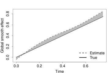
Figure 1: Example of an estimate obtained using the proposed approach (dashed curve) of a global time effect $g_{0}(t)=t$ (solid line). Grey area represents the divergence between the true and estimated effects, measured by the L2-norm of their difference.

The formulation of the model (13) means that the effects are identifiable only up to an additive constant, and thus that the intensity process (3) can only be recovered up to the multiplicative constant $\lambda_{0}$. In the generalized additive modelling implementations, this is handled using an appropriate re-parametrization by means of a centering constraint (Wood, 2017, Section 5.4.1), leading to estimates of smooth terms which are centered around zero. If one is interested in recovering the underlying speed of the event process, the constant $\lambda_{0}$ can be estimated by fitting a linear model to the values of the Breslow estimator at the event times. Indeed, after having accounted for all the estimated effects, the residual cumulative baseline hazard is a linear function of time passing through zero with slope equal to $\lambda_{0}$. In the special case when there is only one global time effect, one can use this estimate of $\lambda_{0}$ to appropriately rescale the plot of the smooth effect and effectively compare it to the true one.

3.4 Shift distribution and estimation uncertainty

The shift distribution in principle does not affect the estimation of the dyadic covariates $\mathbf{f}$, but it does affect the precision of the estimates the global covariates. Clearly, a zero shift would result in an infinite variance. In this section we investigate the relation between the shift distribution used, the variance of the global covariates and the resulting uncertainty around the estimated effects $\mathbf{g}$.

Each effect included as a smooth term in (3) is expressed as a linear combination of a particular set of basis functions $\{b_{j}\}_{j=1}^{B}$. For simplicity, we consider a single global covariate $x(t)$ and no dyadic effects,

$$\lambda_{sr}(t)=\lambda_{0}\exp\left\{\sum_{j=1}^{B}\theta_{j}b_{j}(x(t))\right\}.$$

In order to evaluate the variance of $\theta_{j}$, we consider one single observation of an event $(t,s,r)$ and its corresponding sampled non-event $(t^{*},s^{*},r^{*})$. The observed information, given as the second derivative of the log-likelihood $\log{\mathcal{L}^{PS}}$ with respect to $\theta_{j}$, is given by

$$-\frac{\partial^{2}\log{\mathcal{L}^{PS}}}{\partial\theta_{j}^{2}} =\big{(}b_{j}^{2}(x(t))\pi+b_{j}^{2}(x(t^{*}))(1-\pi)\big{)}-\big{(}b_{j}(x(t))\pi+b_{j}(x(t^{*}))(1-\pi)\big{)}^{2}$$

$$=\mathbb{V}B_{j},$$

where $\pi=\exp\{\sum_{j}\theta_{j}b_{j}(x(t))\}/(\exp\{\sum_{j}\theta_{j}b_{j}(x(t))\}+\exp\{\sum_{j}\theta_{j}b_{j}(x(t^{*}))\})$. The information about $\theta_{j}$ can be seen as the variance of a random variable $B_{j}$ taking value $b_{j}(x(t))$ with probability $\pi$ and $b_{j}(x(t^{*}))$ with probability $1-\pi$. This is directly related to the variability of the shifts, when we consider the definition of the non-event time with respect to the event time, namely $t^{*}=t+h_{sr}-h_{s^{*}r^{*}}$. Given the continuity of the basis functions, the information increases when the shift $\Delta h=\absolutevalue{h_{sr}-h_{s^{*}r^{*}}}$ increases. From this insight, we conclude that the shift distribution should be large. We will validate this empirically in the simulation study, as well as checking the robustness of the estimation when the average shift size increases.

4 Simulation study

In this section, we investigate the effectiveness of the proposed approach by means of a simulation study. In particular, we look closely at how the sample size (number of events), network size (number of nodes) and shift distribution (average shift) affect the performance of our method.

The choice of the variables used to model the intensity processes is made such that a variety of types — global and non-global, node-specific and dyadic, exogenous and endogenous, time dependent and not — are considered. In particular, letting $\mathcal{S}=\mathcal{C}=\{1,\dots,p\}$, we consider the following intensity process

$$\lambda_{sr}(t)=\begin{cases}\exp\{t+\beta_{1}x_{s}+\beta_{2}x_{sr}+\beta_{\text{rep}}x_{\text{rep},sr}(t)+\beta_{0}x(t)\},&\;s\neq r\\ 0,&\;s=r\end{cases}$$ (14)

where $g_{0}(t)=t$ is the global time effect, $x_{\text{rep},sr}(t)$ is a binary endogenous variable representing whether the pair $(s,r)$ occurred at least once up to time $t$ (repetition), $x_{s}$ is a sender-specific exogenous variable associated to the sender, with $x_{s}\sim N(5,1)$, for $s=1\ldots,p$, $x_{sr}$ is a dyadic exogenous covariate defined by $x_{sr}=|x_{s}-x_{r}|$, while $x(t)$ is a global covariate defined as a time-dependent piecewise constant function with some periodicity (exact definition can be found in the Supplementary Materials). The true regression coefficients are set to

$$\beta_{1}=0.5,\ \beta_{2}=-1,\ \beta_{\text{rep}}=1.5,\ \beta_{0}=-0.7.$$

To sample relational events according to the intensity processes $\lambda_{sr}$ defined above, we simulate the counting process $\mathbf{N}$ as an inhomogeneous Poisson process via the $\tau$-leap algorithm (Gillespie, 2001). A detailed description of how we use this algorithm can be found in the Supplementary Materials. Briefly, inter-arrival times between successive events are generated from an exponential distribution by assuming a constant rate in the corresponding infinitesimal time interval of length $\tau$. For each event time obtained in this way, we then use a multinomial distribution to sample the pair that is due to occur from the risk set. In the sampling, we do not allow self-loops and assume that all other pairs are constantly at risk of happening.

For the construction of the time-shifted event process, we consider exponentially distributed shifts with a mean proportional to the average simulated event time according a proportionality constant $\nu$. Estimation of the parameters via the partial likelihood (11) is performed using the gam function from the R package mgcv, using regression terms for each covariate and a thin plate regression spline of rank 10 for the global time effect $g_{0}$ (Wood, 2003). Mean-prediction error is used for the optimal choice of the smoothing parameter.

We fix the sample size to $n=3000$ events, the network size to $p=15$ nodes and the mean shift equal to the average simulated event ($\nu=1$). We then consider 3 settings where we vary one of these parameters in turn, while keeping the other two fixed. For each setting, we perform 100 simulations from the process and summarise the results in terms of estimation of the regression coefficients of the individual covariates $\beta$ and of the residual global time effect $g_{0}(t)$. For the latter, we calculate the $L2$-norm of the difference between the true and estimated effect over the observed time period.

Effect of number of events.

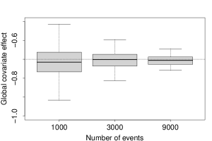
(a)

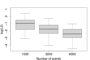
(b)

Figure 2: Results across 100 simulations with $p=15$, $\nu=1$ and $n\in\{1000,3000,9000\}$. As the number of events $n$ increases, (a) the global covariate effect $\beta_{0}$ is centered around the true value (dotted line) and its precision increases (b) the L2-norm (in log-scale) of the difference between the true and estimated global time effect $g_{0}(t)$ decreases.

Figure 2 shows the estimation results for increasing values of the number of events $n\in\{1000,3000,9000\}$ across 100 replications. Figure 2(a) shows a boxplot of the estimates of the regression coefficient of the global covariate $\beta_{0}$. The figure shows how the estimates are centered around the true value (dotted line) and the uncertainty around the estimates decreases as the number of events increases. Similar plots are obtained for the other covariates and are reported in the Supplementary Materials. A similar behavior is observed in Figure 2(b) for the residual global time effect $g_{0}(t)$. As $n$ increases, the estimated function approaches the true function, as shown by a decreasing L2-norm of the differences between the two functions.

Effect of number of nodes.

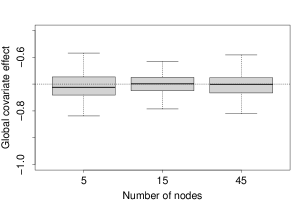
(a)

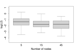
(b)

Figure 3: Results across 100 simulations with $n=3000$, $\nu=1$ and $p\in\{5,15,45\}$. An increasing number of nodes $p$ does not have a strong effect on either (a) estimation of the global covariate effect $\beta_{0}$ or (b) estimation of the global time effect $g_{0}(t)$.

Figure 3 shows the results for increasing values of the number of nodes $p\in\{5,15,45\}$ across 100 replications. Differently to the previous results, we find no strong effect of the number of nodes on either the estimates of the global covariate effect (Figure 3(a)) or of the global time effect (Figure 3(b)).

Effect of shift distribution

Figure 4 shows the results for increasing values of $\nu\in[0.001,1000]$, that is when generating the shifts using a shift distribution with an increasing mean. Across $100$ simulations, Figure 4(a) shows good results for intermediate values of $\nu$ but a higher uncertainty in the estimation of $\beta_{0}$ for the smallest and the largest average shift value. A similar behaviour is observed for the estimation of the global time effect (Figure 4(b)), with an estimation error that decreases the greater the shifts are on average, but that starts to deteriorate for too large shifts. The reason behind this behaviour at the two extremes is different in the two cases. For too small shifts, the behaviour is supported by the theoretical results investigated in Section 3.4 and is particularly accentuated by the temporal resolution used to define the piecewise constant global covariate $x(t)$. Indeed, for too small shifts, the event and non-event times are frequently so close to each other that $x(t)$ has the same values when evaluated at these two time points. This results in many structural zeros in the likelihood when considering the difference between the covariate of the event and of the non-event, which negatively impacts the ability of the method to effectively estimate $\beta_{0}$. On the other hand, when shifts are too large, it occurs very often (roughly for 80% of the observations in the simulation study) that the risk set in the shifted process at a certain event time is only composed of the pair occurring, making it impossible to sample a non-event and making a large percentage of the observations uninformative when it comes to estimation. Such a situation clearly results in a considerable reduction in the effective sample size, which negatively impacts the precision of the estimation procedure.

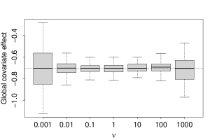
(a)

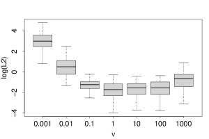
(b)

Figure 4: Results across 100 simulations with $n=3000$, $p=15$ and $\nu\in[0.001,1000]$. Too small or too large shifts have a negative effect both on (a) estimation of the global covariate effect $\beta_{0}$ and (b) estimation of the global time effect $g_{0}(t)$. No effect for intermediate values of $\nu\in[0.1,100]$.

5 Bike sharing in Washington D.C.

In this section, we use the proposed approach to model bike sharing data from Washington D.C. The aim is to investigate the effect that global factors, like temperature and precipitation, in addition to a number of node-specific and dyadic covariates of interest, have on the rate of bike shares during the time period considered.

The data are available at https://www.capitalbikeshare.com/system-data. It reports information about bike shares among more than 1300 locations in D.C in the period July 9th-31st, 2023. The locations are the nodes of the network, while an edge goes from a station $s$ to another station $r$ at time $t$ if a bike is taken from station $s$ at time $t$ and is then left at station $r$. We do not account for the duration of the ride, effectively assuming that the ride is instantaneous. In total, almost 350k events are recorded.

We propose the following model

$$\lambda_{sr}(t) =\lambda_{0}\exp\{g_{0}(t)+g_{\text{temp}}(x^{\text{(temp)}}(t))+g_{\text{prec}}(x^{\text{(prec)}}(t))+g_{\text{tod}}(x^{\text{(ToD)}}(t))$$

$$+x_{s}^{\text{(comp)}}\beta+x_{r}^{\text{(comp)}}\gamma$$ (15)

$$+f_{\text{dist}}(x_{sr}^{\text{(dist)}})+f_{\text{rep}}(x_{sr}^{\text{(rep)}}(t))+f_{\text{rec}}(x_{sr}^{\text{(rec)}}(t))\}.$$

which includes a variety of variables — both global and node/edge-specific — that we describe below:

• Global covariates. To investigate the role weather plays in the dynamics of bike shares, we include in the model a smooth effect of temperature $x^{\text{(temp)}}(t)$, measured in °C, and one for precipitation $x^{\text{(prec)}}(t)$, measured in mm and log-transformed to stabilize its variance. Weather information is taken from https://www.wunderground.com/. Since the data are available hourly, we consider these two functions as piecewise constant. In addition to the usual global time effect $g_{0}(t)$, we also account for another smooth temporal effect, involving time of day. In particular, the covariate $x^{\text{(ToD)}}(t)$ returns a numeric value between 0 and 24 according to the hour of day corresponding to time $t$.

• Node-level covariates. In order to assess the impact that competition between bike stations has on the rate, we include two variables $x_{s}^{\text{(comp)}}$ and $x_{r}^{\text{(comp)}}$, which are defined as the distance between station $s$ (or $r$, respectively) and its closest bike station, measured in biking minutes. High values for these covariates indicate that station $s$ (or similarly $r$) have less competition within the geographical area they are located in.

• Dyadic covariates. We model a smooth effect for the distance between stations $x_{sr}^{\text{(dist)}}$, measured in biking minutes and log-transformed. The distances are obtained from Open Street Maps using the R package osrm. Additionally, we account for two network effects: a reciprocity effect, related to the tendency of observing a bike share going through a particular bike route given that one was previously observed in the opposite direction, and a repetition effect, related to the propensity of observing a bike share on a specific route, given that another one previously occurred along the same route. We do this by defining smooth effects of the following two endogenous covariates

  $$x_{sr}^{\text{(rep)}}(t) =\exp\{-\delta_{sr}^{\text{(rep)}}(t)/2m_{\text{rep}}\},~{}~{}\delta_{sr}^{\text{(rep)}}(t)=\min_{t_{k}<t;s_{k}=s;r_{k}=r}t-t_{k}$$

  $$x_{sr}^{\text{(rec)}}(t) =\exp\{-\delta_{sr}^{\text{(rec)}}(t)/2m_{\text{rec}}\},~{}~{}\delta_{sr}^{\text{(rec)}}(t)=\min_{t_{k}<t;s_{k}=r;r_{k}=s}t-t_{k}$$

  where $\delta_{sr}^{\text{(rep)}}$ and $\delta_{sr}^{\text{(rec)}}$ are the elapsed times since the same previous event or the reciprocal event to $(s,r)$, respectively, occurred. The values $m_{\text{rep}}$ and $m_{\text{rec}}$ are the medians of $\delta_{sr}^{\text{(rep)}}$ and $\delta_{sr}^{\text{(rec)}}$, respectively. The exponential transformation guards against the case of elapsed times being infinity, when the relevant event was never observed in the past, while the median makes sure that $\delta$ quantities that are not infinity do not end up being mapped to 0. The resulting variables have values between 0 and 1; the closer to zero, the further apart in time the previous same or reciprocal event is from the current event under consideration, while events repeated or reciprocated closer in time correspond to values for these variables close to 1.

For the construction of the time-shifted event process, we consider exponentially distributed shifts with a mean equal to the average event time ($\nu=1$). Estimation of the parameters via the partial likelihood (11) is performed using the gam function from the R package mgcv. All smooth effects are handled using thin plate regression splines of rank 10, with the exception of repetition and reciprocity, for which we consider rank 20, and the time-of-day, for which we use cyclic penalized cubic regression splines constructed over 10 evenly spaced knots (Wood, 2017).

(a)

(b)

(c)

	Coef.	S.E.	$p$-value
sender comp. $\beta$	-0.2145	0.0103	$<0.0001$
receiver comp. $\gamma$	-0.1885	0.0101	$<0.0001$

(d)

Figure 5: Effects of global and node-level covariates on bike sharing rate: (a) The warmer it is the higher the rate of bike sharing, unless it is too hot. (b) Precipitation disincentivizes bike sharing. (c) Daylight and working hours have a higher propensity to bike sharing, with an increase at the beginning (4am-9am) and at the end (6pm) of the working day. (d) Both competition parameters are negative: even though other stations are close by, this does not increase the bike share intensity, on the contrary.

Figure 5 plots the estimated smooth effects associated to the global covariates. As expected, Figure 5(a) shows how the occurrence of bike routes generally increases as the temperature increases, but starts decreasing when the temperature becomes too high. Similarly, Figure 5(b) shows how precipitation discourages bike sharing. In addition to weather, time of day plays an important role in describing the tendency to rent a bike, with daylight and working hours being associated to a higher rate of bike sharing. Indeed, Figure 5(c) shows how the intensity of bike shares between stations decreases at night (between midnight and 4am, and after 7 pm) and increases during the day, particularly between 4 and 9 am, which is most likely when people get to work, and around 6 pm, which is when they return from work.

(a)

(b)

Figure 6: Effects of 2 dyadic covariates on bike sharing rate: (a) Bike shares have a daily repeating pattern, describing the tendency to go along the same route every day. (b) The further apart two bike stations are, the less likely is a bike share between them.

Figure 6 plots the estimated smooth effects associated to two dyadic covariates, repetition and distance. The other dyadic effect, reciprocity, as well as the global time effect, are included in the Supplementary Materials. Figure 6(a) shows a daily repeating pattern, with a considerable increase at 24 hours, describing the tendency to go along the same bike route on a daily basis. Interestingly, even though repetition is defined as an endogenous effect, it actually ends up capturing a daily “exogenous” pattern. As for distance (Figure 6(b)), there is generally a decreasing trend as distance increases, which is to be expected, though we do not detect any decreasing effect for very short distances, where we might have expected people to not use bikes.

In connection with the geographical location of bike stations, Figure 5(d) reports the regression coefficients associated to the two node-level covariates describing the sender’s and receiver’s competition effects, respectively. As the variables are defined as distances between a sender/receiver station and its closest station, the negative estimates suggest a “negative competition” scenario. This could be explained by the lack of a sufficient number of stations for the actual volume of bike shares in the area. Despite the close vicinity of other bike sender or receiver stations, the traffic is actually higher than for those stations that do no have other stations nearby.

6 Conclusions

Relational event models provide an ideal framework for analysing sequences of time-stamped interactions in a variety of applied settings. Existing inferential techniques only allow to investigate how node- or edge-specific covariates are able to explain the underlying dynamics of interactions. In this paper, we propose an extension of relational event models with the inclusion of global covariates, that is covariates that are time-dependent but constant across interacting pairs. As the contribution of these covariates would normally drop out of the partial likelihood, we propose a time-shifted version of the original event process, from which we are able to recover the effect of all kinds of variables, including global ones.

In order to scale the inferential approach to large dynamic networks, we propose the use of nested case-control sampling. In the specific case of one non-event sampled from the risk set at each event time, we show how the partial likelihood is that of a degenerate logistic additive model, for which efficient implementations are available that allow the inclusion of fixed, time-varying and random effects.

A simulation study shows the effectiveness of the proposed approach in recovering both global and non-global effects and sheds light into the role played by sample size, network size and the shift distribution on the performance of the approach. Finally, we show the applicability of the proposed methodology on the modelling of bike sharing data from Washington D.C., where global covariates, such as weather conditions and time of the day, are found to play an important role in describing the rate of bike sharing between two stations.

Code availability.

All the code for the simulation and empirical analysis of bike sharing data can be found at the GitHub repository page.

References

- Bianchi et al. (2023) Bianchi, F., E. Filippi-Mazzola, A. Lomi, and E. C. Wit (2023). Relational event modeling. Annual Review of Statistics and Its Application.
- Bianchi and Lomi (2023) Bianchi, F. and A. Lomi (2023). From ties to events in the analysis of interorganizational exchange relations. Organizational Research Methods 26(3), 524–565.
- Borgan et al. (1995) Borgan, Ø., L. Goldstein, and B. Langholz (1995). Methods for the analysis of sampled cohort data in the cox proportional hazards model. The Annals of Statistics 23(5), 1749–1778.
- Boschi et al. (2023) Boschi, M., R. Juozaitienė, and E. C. Wit (2023). Smooth alien species invasion model with random and time-varying effects. arXiv:2304.00654 [stat.AP].
- Brandes et al. (2009) Brandes, U., J. Lerner, and T. A. B. Snijders (2009). Networks evolving step by step: Statistical analysis of dyadic event data. 2009 International Conference on Advances in Social Network Analysis and Mining, 200–205.
- Breslow (1972) Breslow, N. E. (1972). Contribution to discussion of paper by dr cox. Journal of the Royal Statistical Society, Series B 34, 216–217.
- Butts (2008) Butts, C. T. (2008). A relational event framework for social action. Sociological Methodology 38(1), 155–200.
- Cox (1972) Cox, D. R. (1972). Regression models and life-tables. Journal of the Royal Statistical Society. Series B (Methodological) 34(2), 187–220.
- Filippi-Mazzola and Wit (2024) Filippi-Mazzola, E. and E. C. Wit (2024, 05). A stochastic gradient relational event additive model for modelling US patent citations from 1976 to 2022. Journal of the Royal Statistical Society Series C: Applied Statistics.
- Gillespie (2001) Gillespie, D. T. (2001). Approximate accelerated stochastic simulation of chemically reacting systems. The Journal of Chemical Physics 115(4), 1716–1733.
- Hastie and Tibshirani (1990) Hastie, T. and R. Tibshirani (1990). Generalized additive models. Chapman & Hall/CRC.
- Juozaitienė et al. (2023) Juozaitienė, R., H. Seebens, G. Latombe, F. Essl, and E. C. Wit (2023). Analysing ecological dynamics with relational event models: The case of biological invasions. Diversity and Distributions 29(10), 1208–1225.
- Juozaitienė and Wit (2022) Juozaitienė, R. and E. C. Wit (2022). Non-parametric estimation of reciprocity and triadic effects in relational event networks. Social Networks 68, 296–305.
- Juozaitienė and Wit (2024) Juozaitienė, R. and E. C. Wit (2024). Nodal heterogeneity can induce ghost triadic effects in relational event models. Psychometrika 89(1), 151–171.
- Kalbfleisch and Prentice (1973) Kalbfleisch, J. D. and R. L. Prentice (1973). Marginal likelihoods based on cox’s regression and life model. Biometrika 60(2), 267–278.
- Kreiss et al. (2023) Kreiss, A., E. Mammen, and W. Polonik (2023). Testing for global covariate effects in dynamic interaction event networks. Journal of Business & Economic Statistics 0(0), 1–12.
- Lerner and Lomi (2023) Lerner, J. and A. Lomi (2023). Relational hyperevent models for polyadic interaction networks. Journal of the Royal Statistical Society Series A: Statistics in Society 186(3), 577–600.
- Perry and Wolfe (2013) Perry, P. O. and P. J. Wolfe (2013). Point process modelling for directed interaction networks. Journal of the Royal Statistical Society. Series B (Statistical Methodology) 75(5), 821––849.
- Uzaheta et al. (2023) Uzaheta, A., V. Amati, and C. Stadtfeld (2023). Random effects in dynamic network actor models. Network Science 11(2), 249–266.
- Vu et al. (2015) Vu, D., P. Pattison, and G. Robins (2015). Relational event models for social learning in moocs. Social Networks 43, 121–135.
- Wood (2003) Wood, S. N. (2003). Thin plate regression splines. Journal of the Royal Statistical Society Series B: Statistical Methodology 65(1), 95–114.
- Wood (2017) Wood, S. N. (2017). Generalized additive models: an introduction with R (Second edition ed.). CRC Press/Taylor & Francis Group.