Towards Unified AI Models for MU-MIMO Communications: A Tensor Equivariance Framework

Abstract

In this paper, we propose a unified framework based on equivariance for the design of artificial intelligence (AI)-assisted technologies in multi-user multiple-input-multiple-output (MU-MIMO) systems. We first provide definitions of multidimensional equivariance, high-order equivariance, and multidimensional invariance (referred to collectively as tensor equivariance). On this basis, by investigating the design of precoding and user scheduling, which are key techniques in MU-MIMO systems, we delve deeper into revealing tensor equivariance of the mappings from channel information to optimal precoding tensors, precoding auxiliary tensors, and scheduling indicators, respectively. To model mappings with tensor equivariance, we propose a series of plug-and-play tensor equivariant neural network (TENN) modules, where the computation involving intricate parameter sharing patterns is transformed into concise tensor operations. Building upon TENN modules, we propose the unified tensor equivariance framework that can be applicable to various communication tasks, based on which we easily accomplish the design of corresponding AI-assisted precoding and user scheduling schemes. Simulation results demonstrate that the constructed precoding and user scheduling methods achieve near-optimal performance while exhibiting significantly lower computational complexity and generalization to inputs with varying sizes across multiple dimensions. This validates the superiority of TENN modules and the unified framework.

I Introduction

The multiple-input-multiple-output (MIMO) technology [1], which serves users using multiple antennas, has become a key technology in wireless communication systems due to its enormous potential for increasing system capacity [2]. Leveraging MIMO technology, the base stations (BSs) in multi-user MIMO (MU-MIMO) systems possess enhanced transmission performance to simultaneously serve multiple users. In such systems, resource allocation schemes such as user scheduling and precoding techniques play a critical role in improving throughput. On the one hand, user scheduling aims to select users from the pool of all users for simultaneous transmission in certain resource elements, with the goal of improving transmission quality. On the other hand, precoding further enhances the potential capacity gains by suppressing user interference. Since the evolution of MU-MIMO technology, numerous excellent scheduling and precoding algorithms have been proposed, such as greedy-based scheduling schemes [3] and weighted minimum mean square error (WMMSE) precoding [4, 5, 6], which play a crucial role in future research.

While conventional transmission schemes in MU-MIMO systems can achieve outstanding performance [4, 3], even approaching the performance limits [7, 8], they usually require iterative computations and high computational complexity. Such issues become increasingly severe in the face of the growing scale of wireless communication systems [9], posing significant obstacles to their application in practical systems. In contrast, artificial intelligence (AI) models possess the potential to accelerate iterative convergence and approximate high-dimensional mappings with lower computational complexity [10, 11], leading to extensive research into AI-assisted transmission schemes [12].

Most AI-assisted transmission schemes treat inputs as structured data, such as image data or vector data, and process them using corresponding neural networks (NNs) [13, 14, 15, 16, 17, 18]. Specifically, building on the optimal closed-form solution derived from WMMSE precoding [4, 19], the authors in [13] utilize fully connected (FC) layers to directly compute key features in optimal solution forms, while similar schemes are proposed with convolutional NN (CNN) in [14] and [15], as channel information can be regarded as image data. Based on CNN, AI-assisted schemes utilizing optimal solution structures have been extended to multiple precoding optimization criteria [16]. With the imperfect channel state information (CSI), [17] and [18] investigated the robust WMMSE precoding algorithms with CNNs. Unlike FC and CNN networks, deep unfolding networks integrate learnable parameters into iterative algorithms to expedite algorithmic convergence [20, 21, 22]. For instance, [20] introduced a matrix-inverse-free deep unfolding network for WMMSE precoding. A similar approach is explored in [21], demonstrating superior performance compared to CNNs. Such approach is further extended to WMMSE precoding design under imperfect CSI conditions [22]. Apart from precoding, there are also some AI-assisted methods for other resource allocation schemes [23, 24, 25]. In [23], FC networks are utilized to extract optimal power allocation schemes from CSI for maximizing sum-rate. Besides, a user scheduling strategy aided by FC networks is proposed in [24], which assigns the most suitable single user for each resource block. Based on edge cloud computing and deep reinforcement learning, the user scheduling strategy in [25] are developed for millimeter-wave vehicular networks. Additionally, there are studies providing deep insights to empower AI-assisted transmission technology [26, 27]. The work in [26] elucidates the shortcomings of AI in solving non-convex problems and presents a framework to address this issue. The authors of [27] investigated the asymptotic spectral representation of linear convolutional layers, offering guidance on the excellent performance of CNNs.

The aforementioned studies typically do not focus on permutation equivariance (abbreviated as equivariance) [28], which entails that permutation of input elements in a model also results in the corresponding permutation of output elements. Such property is inherent to MU-MIMO systems and endows AI-assisted transmission technologies with the potential advantages like parameter sharing [29]. Benefiting from its modeling of graph topology, graph NN (GNN) possess the capability to exploit this property, thus being employed in the design of transmission schemes and demonstrating outstanding performance [30]. In [31], the significance of topological information for transmission within an interference management framework is investigated. The GNNs used for wireless resource management is proposed in [32], which develops equivariance and thereby achieves generalization across varying numbers of users. In addition, the authors in [33] model the link network between BS antennas and terminals as a bipartite graph, thereby achieving generalization across varying numbers of users and BS antennas. Similarly, GNNs with different iteration mechanisms are proposed for precoding design in [34] and [35]. By crafting refined strategies for updating node features, a GNN satisfying equivariance across multiple node types is devised for hybrid precoding in [36]. The proposed methodology demonstrates exceptional performance and scalability, paving the way for GNN-assisted transmission design. Furthermore, aiming to maximize the number of served users, a GNN-based joint user scheduling and precoding method is investigated in [37].

Existing efforts in developing inherent properties in wireless communication systems are limited to GNN, requiring intricate node modeling and the construction of node update strategy during the design process. Therefore, with the increasing trend of incorporating multiple device types in communication systems [38], the design of schemes based on this approach may become increasingly complicated. Furthermore, although existing work has made outstanding contributions in developing equivariance in communication systems [36, 39, 40], there is little effort on investigating concise and unified frameworks to develop diverse equivariances such as multidimensional equivariance [41], higher-order equivariance [42], and invariance [43] in such systems.

In this paper, we focus on the development of these properties and proposed a unified framework for exploiting them in MU-MIMO systems. The major contributions of our work are summarized as follows:

• We establish the new concept, tensor equivariance (TE), which can be utilized for capturing properties such as multidimensional equivariance, high-order equivariance, and invariance. Using the design of precoding and user scheduling as an example, we prove the inherent TE within the mappings from CSI to optimal precoding tensors, precoding auxiliary tensors, and scheduling indicators. Similar process can be extended to other techniques of wireless communication system.

• We propose the TE framework to fully and efficiently exploit TE. Such a framework comprises stages such as input tensor construction, exploration of TE, and output layer construction, facilitating the effortless design of NNs for exploiting TE. By utilizing such framework, we easily accomplish the design of corresponding AI-assisted precoding and user scheduling schemes.

• TE framework is unified, capable of addressing various tasks beyond precoding and user scheduling. The framework comprises multiple TENN modules, which are plug-and-play and can be reconfigured for different task within MU-MIMO systems. Compared to conventional NN modules, these offer advantages such as low complexity, parameter sharing, and generalizability to inputs with varying sizes across multiple dimensions.

This paper is structured as follows: In Section II, we put forward TE in MU-MIMO systems. Section III proposes plug-and-play TENN modules. Section IV investigates the unified TE framework. Section V reports the simulation results, and the paper is concluded in Section VI.

Notation: $(\cdot)^{-1},(\cdot)^{T},(\cdot)^{H}$ denote the inverse, transpose, and the transpose-conjugate operations, respectively. $x$, ${\bf x}$, ${\bf X}$, and ${\bm{\mathsfit{X}}}$ respectively denote a scalar, column vector, matrix, and tensor. $\real(\cdot)$ and $\Im(\cdot)$ represent the real and imaginary part of a complex scalars, vector or matrix. $j=\sqrt{-1}$ denote imaginary unit. $\in$ denotes belonging to a set. $\mathcal{A}\backslash\mathcal{B}$ means objects that belong to set $\mathcal{A}$ but not to $\mathcal{B}$. $|\mathcal{A}|$ represents the cardinality of set $\mathcal{A}$. ${\bf I}_{K}$ denotes $K\times K$ identity matrix. ${\bf 1}$ denotes the suitable-shape tensor with all elements being ones. $\left\|\cdot\right\|_{2}$ denotes $l_{2}$-norm. ${\rm det}({\bf A})$ represents the determinant of matrix ${\bf A}$. ${\rm blkdiag}\{{\bf A}_{1},...,{\bf A}_{K}\}$ represents a block diagonal matrix composed of ${\bf A}_{1},...,{\bf A}_{K}$. We use ${\bm{\mathsfit{X}}}_{[m_{1},...,m_{N}]}$ to denote the indexing of elements in tensor ${\bm{\mathsfit{X}}}\in\mathbb{R}^{M_{1}\times\cdots\times M_{N}}$. $[{\bm{\mathsfit{A}}}_{1},...,{\bm{\mathsfit{A}}}_{K}]_{S}$ denotes the tensor formed by stacking ${\bm{\mathsfit{A}}}_{1},...,{\bm{\mathsfit{A}}}_{K}$ along the $S$-th dimension. $[\cdot]_{0}$ denotes the concatenation of tensors along a new dimension, i.e., ${\bm{\mathsfit{A}}}_{[n,:,\cdots]}={\bm{\mathsfit{B}}}_{n},\ \forall n$ when ${\bm{\mathsfit{A}}}=[{\bm{\mathsfit{B}}}_{1},...,{\bm{\mathsfit{B}}}_{N}]_{0}$. We define the product of tensor ${\bm{\mathsfit{X}}}\in\mathbb{R}^{M_{1}\times\cdots\times M_{N}\times D_{X}}$ and matrix ${\bf Y}\in\mathbb{R}^{D_{X}\times D_{Y}}$ as $({\bm{\mathsfit{X}}}\times{\bf Y})_{[m_{1},...,m_{N},:]}={\bm{\mathsfit{X}}}_{[m_{1},...,m_{N},:]}{\bf Y}$. The Hadamard product of tensor ${\bm{\mathsfit{X}}}\in\mathbb{R}^{M_{1}\times\cdots\times M_{N}\times D_{X}}$ and matrix ${\bf Y}\in\mathbb{R}^{M_{N}\times D_{X}}$ is defined as $({\bm{\mathsfit{X}}}\odot{\bf Y})_{[m_{1},...,m_{N-1},:,:]}={\bm{\mathsfit{X}}}_{[m_{1},...,m_{N-1},:,:]}\odot{\bf Y}$. The Kronecker product of tensor and matrix is defined as $({\bm{\mathsfit{X}}}\otimes_{n}{\bf Y})_{[m_{1},...,m_{n-1},:,:,m_{n+2},...,m_{N}]}={\bm{\mathsfit{X}}}_{[m_{1},...,m_{n-1},:,:,m_{n+2},...,m_{N}]}\otimes{\bf Y}$.

II Tensor Equivariance in MU-MIMO systems

In this section, we first introduce the concept of TE, and subsequently prove TE inherent in the design of precoding and user scheduling in MU-MIMO systems.

II-A Tensor Equivariance

We collectively term the equivariance to tensors, including multidimensional equivariance, high-order equivariance, and invariance, as TE. Below, we will provide their specific definitions.

The permutation $\pi_{N}$ denotes a shuffling operation on the index $[1,...,N]$ of a length-$N$ vector under a specific pattern (or referred to as bijection from the the indices set ${\mathcal{N}}=\{1,2,...,N\}$ to ${\mathcal{N}}$), with the operator $\circ$ denoting its operation, and $\pi_{N}(n)$ represents the result of mapping $\pi_{N}$ on index $n$. For example, if $\pi_{3}\circ[x_{1},x_{2},x_{3}]=[x_{2},x_{3},x_{1}]$, then $\pi_{3}(1)=2$, $\pi_{3}(2)=3$, and $\pi_{3}(3)=1$ [28]. For tensor, we further extend the symbol $\circ$ to $\circ_{m}$, representing the permutation of dimension $m$ in the tensor by $\pi$. For instance, if $\pi_{3}\circ_{2}{\bm{\mathsfit{X}}}={\bm{\mathsfit{X}}}^{\prime}$, then ${\bm{\mathsfit{X}}}^{\prime}_{[:,1,:]}={\bm{\mathsfit{X}}}_{[:,2,:]}$, ${\bm{\mathsfit{X}}}^{\prime}_{[:,2,:]}={\bm{\mathsfit{X}}}_{[:,3,:]}$, and ${\bm{\mathsfit{X}}}^{\prime}_{[:,3,:]}={\bm{\mathsfit{X}}}_{[:,1,:]}$. We define the set of all permutations for $[1,...,N]$ as ${\mathbb{S}}_{N}$, which is also referred to as the symmetric group [44, 45]. Then, we have $\pi_{N}\in{\mathbb{S}}_{N}$ and $|{\mathbb{S}}_{N}|=N!$.

The mapping $f:\mathbb{R}^{M_{1}\times\cdots\times M_{N}\times D_{X}}\to\mathbb{R}^{M_{1}\times\cdots\times M_{N}\times D_{Y}}$ exhibits multidimensional ($N$-dimensional) equivariance when it satisfies

$$f({\pi_{M_{n}}}\!\circ_{n}\!{\bm{\mathsfit{X}}})={\pi_{M_{n}}}\!\circ_{n}\!f({\bm{\mathsfit{X}}}),\ \forall{\pi_{M_{n}}}\in{\mathbb{S}}_{M_{n}},\forall n\in\mathcal{N}.$$ (1)

where $\mathcal{N}\in\{1,...,N\}$. This indicates that upon permuting a certain dimension in $\mathcal{N}$ of the input, the order of items in the corresponding dimension of the output will also be permuted accordingly [11, 46], which aligns with those described in [41, 47].

We refer the mapping $f:\mathbb{R}^{\scriptsize{\overbrace{M\times\cdots\times M}^{p}}\times D_{X}}\to\mathbb{R}^{\scriptsize{\overbrace{M\times\cdots\times M}^{q}}\times D_{Y}}$ exhibits high-order ($p$-$q$-order) equivariance when it satisfies

$$f({\pi_{M}}\!\circ_{[1,...,p]}\!{\bm{\mathsfit{X}}})={\pi_{M}}\!\circ_{[1,...,q]}\!f({\bm{\mathsfit{X}}}),\ \forall{\pi_{M}}\in{\mathbb{S}}_{M},$$ (2)

where $\pi_{M}\circ_{[1,...,p]}$ represents performing the same permutation $\pi_{M}$ on the dimensions $1,...,p$, respectively. The above equation expresses the equivariance of the mapping $f$ with respect to identical permutations across multiple dimensions, which originates from the descriptions in [48, 42].

The mapping $f:\mathbb{R}^{M_{1}\times\cdots\times M_{N}\times D_{X}}\to\mathbb{R}^{D_{Y}}$ exhibits multidimensional ($N$-dimensional) invariance when it satisfies [43]

$$f({\pi_{M_{n}}}\!\circ_{n}\!{\bm{\mathsfit{X}}})=f({\bm{\mathsfit{X}}}),\ \forall{\pi}_{M_{n}}\in{\mathbb{S}}_{M_{n}},\ \forall n\in\mathcal{N}.$$ (3)

The above equation illustrates that permuting the indices of the input across the dimensions contained in $\mathcal{N}$ does not affect the output of $f$. The properties described above are derived from the invariance in [28].

Next, we will exemplify the design of precoding and user scheduling schemes to reveal the TE commonly present in the design of MU-MIMO systems.

II-B Tensor Equivariance in Precoding Design

Consider an MU-MIMO system where a BS equipped with $N_{\rm T}$ antennas transmits signals to $K$ users equipped with $N_{\rm R}$ antennas. The optimization problem of sum-rate maximization can be formulated as [19]:

$$\begin{split}&\max_{{\bm{\mathsfit{W}}}}\ \sum_{k=1}^{K}R_{k}({\bm{\mathsfit{H}}},{\bm{\mathsfit{W}}},\sigma^{2})\ \ {\rm s.t.}\ \sum_{k=1}^{K}{\rm Tr}\left({\bf W}_{k}{\bf W}^{H}_{k}\right)\leq P_{\rm T},\end{split}$$ (4)

where ${\bm{\mathsfit{H}}}=[{\bf H}_{1},...,{\bf H}_{K}]_{0}\in\mathbb{C}^{K\times N_{\rm R}\times N_{\rm T}}$, ${\bm{\mathsfit{W}}}=[{\bf W}_{1},...,{\bf W}_{K}]_{0}\in\mathbb{C}^{K\times N_{\rm R}\times N_{\rm T}}$, ${\bf H}_{k}\in{\mathbb{C}}^{N_{\rm R}\times N_{\rm T}}$ denotes the channel from the BS to the $k$-th user, ${\bf W}_{k}\in{\mathbb{C}}^{N_{\rm R}\times N_{\rm T}}$ denotes the precoding matrix of the $k$-th user, $P_{\rm T}$ represents the fixed transmit power, $\sigma^{2}$ is the noise power, $R_{k}({\bm{\mathsfit{H}}},{\bm{\mathsfit{W}}},\sigma^{2})=\log{\rm det}\left({\bf I}_{k}+{\bf W}_{k}{\bf H}^{H}_{k}{\bm{\Omega}}^{-1}_{k}{\bf H}_{k}{\bf W}^{H}_{k}\right)$ is the rate, and ${\bm{\Omega}}_{k}=\sigma^{2}{\bf I}+\sum_{i=1,i\neq k}^{K}{\bf H}_{k}{\bf W}^{H}_{i}{\bf W}_{i}{\bf H}^{H}_{k}\in{\mathbb{C}}^{N_{\rm R}\times N_{\rm R}}$ is the effective Interference-plus-noise covariance matrix. It can be concluded that (4) is a problem for ${\bm{\mathsfit{W}}}$ based on available CSI ${\bm{\mathsfit{H}}}$ and $\sigma^{2}$.

To simplify subsequent expressions, we define $\langle{\bm{\mathsfit{W}}},\{{\bm{\mathsfit{H}}},\sigma^{2}\}\rangle_{\rm P}$ as a pairing of precoding and CSI for problem (4). Furthermore, the objective function achieved by ${\bm{\mathsfit{W}}}$ and $\{{\bm{\mathsfit{H}}},\sigma^{2}\}$ in problem (4) is denoted as ‘the objective function of $\langle{\bm{\mathsfit{W}}},\{{\bm{\mathsfit{H}}},\sigma^{2}\}\rangle_{\rm P}$’. On this basis, the property of optimization problem (4) is as follows.

Proposition 1.

The objective function of $\langle{\bm{\mathsfit{W}}},\{{\bm{\mathsfit{H}}},\sigma^{2}\}\rangle_{\rm P}$ is equal to those of $\langle\pi_{K}\circ_{1}{\bm{\mathsfit{W}}},\{\pi_{K}\circ_{1}{\bm{\mathsfit{H}}},\sigma^{2}\}\rangle_{\rm P}$, $\langle\pi_{N_{\rm R}}\circ_{2}{\bm{\mathsfit{W}}},\{\pi_{N_{\rm R}}\circ_{2}{\bm{\mathsfit{H}}},\sigma^{2}\}\rangle_{\rm P}$, and $\langle\pi_{{N_{\rm T}}}\circ_{3}{\bm{\mathsfit{W}}},\{\pi_{{N_{\rm T}}}\circ_{3}{\bm{\mathsfit{H}}},\sigma^{2}\}\rangle_{\rm P}$, for all $\pi_{K}\in{\mathbb{S}}_{K}$, $\pi_{N_{\rm R}}\in{\mathbb{S}}_{N_{\rm R}}$, and $\pi_{{N_{\rm T}}}\in{\mathbb{S}}_{N_{\rm T}}$. Specifically, if $\langle{\bm{\mathsfit{W}}}^{\star},\{{\bm{\mathsfit{H}}},\sigma^{2}\}\rangle_{\rm P}$ achieves the optimal objective function, then $\langle\pi_{K}\circ_{1}{\bm{\mathsfit{W}}}^{\star},\{\pi_{K}\circ_{1}{\bm{\mathsfit{H}}},\sigma^{2}\}\rangle_{\rm P}$, $\langle\pi_{N_{\rm R}}\circ_{2}{\bm{\mathsfit{W}}}^{\star},\{\pi_{N_{\rm R}}\circ_{2}{\bm{\mathsfit{H}}},\sigma^{2}\}\rangle_{\rm P}$, and $\langle\pi_{{N_{\rm T}}}\circ_{3}{\bm{\mathsfit{W}}}^{\star},\{\pi_{{N_{\rm T}}}\circ_{3}{\bm{\mathsfit{H}}},\sigma^{2}\}\rangle_{\rm P}$ can also achieve their optimal objective functions.

Proof.

See Appendix A.

More clearly, we define $G_{\rm P}(\cdot)$ as a mapping from CSI to one of the optimal precoding schemes for (4), i.e., $G_{\rm P}({\bm{\mathsfit{H}}},\sigma^{2})={\bm{\mathsfit{W}}}^{\star}$. Then, based on Proposition 1, the following equations hold when problem (4) has a unique optimal solution.

$$G_{\rm P}({\pi_{K}}\!\circ_{1}\!{\bm{\mathsfit{H}}},\sigma^{2})={\pi_{K}}\!\circ_{1}\!{\bm{\mathsfit{W}}}^{\star},\ \forall{\pi}_{K}\in{\mathbb{S}}_{K},$$ (5a)

$$G_{\rm P}({\pi_{N_{\rm R}}}\!\circ_{2}\!{\bm{\mathsfit{H}}},\sigma^{2})={\pi_{N_{\rm R}}}\!\circ_{2}\!{\bm{\mathsfit{W}}}^{\star},\ \forall{\pi}_{N_{\rm R}}\in{\mathbb{S}}_{N_{\rm R}},$$ (5b)

$$G_{\rm P}({\pi_{N_{\rm T}}}\!\circ_{3}\!{\bm{\mathsfit{H}}},\sigma^{2})={\pi_{N_{\rm T}}}\!\circ_{3}\!{\bm{\mathsfit{W}}}^{\star},\ \forall{\pi}_{N_{\rm T}}\in{\mathbb{S}}_{N_{\rm T}}.$$ (5c)

If the optimization problem has multiple optimal solutions, it can be proven that the optimization problem for the permuted CSI also has the same number of optimal solutions, and they correspond one-to-one in the manner described by the equations above. In this case, $G_{\rm P}(\cdot)$ can be regarded as a mapping for one of the optimal solutions of the optimization problem.

For problem (4), iterative algorithms based on optimal closed-form expressions can achieve outstanding performance and have garnered considerable attention [4, 19]. Consequently, we further analyze the equivariance inherent in the design of precoding schemes based on optimal closed-form expressions. The well-known solution to problem (4) can be obtained through the following expression [4, 5, 6]

$$\begin{split}{\bf W}\!=\!\gamma{\tilde{\bf W}},{\tilde{\bf W}}\!=\!{\bf H}^{H}{\bf A}^{H}{\bf U}\left(\mu{\bf I}_{MK}\!+\!{\bf A}{\bf H}{\bf H}^{H}{\bf A}^{H}{\bf U}\right)^{-1},\\ \gamma=\sqrt{{P_{\rm T}}/{{\rm Tr}({\tilde{\bf W}}{\tilde{\bf W}}^{H})}},\ \mu={{\rm Tr}\left({\bf U}{\bf A}{\bf A}^{H}\right)}\sigma^{2}/{P_{\rm T}},\end{split}$$ (6)

where

$${\bf W}=[{\bf W}_{1},...,{\bf W}_{K}]^{T}\in{\mathbb{C}}^{N_{\rm T}\times KN_{\rm R}},$$ (7)

$${\bf U}={\rm blkdiag}\{{\bf U}_{1},...,{\bf U}_{K}\}\in{\mathbb{C}}^{KN_{\rm R}\times KN_{\rm R}},$$ (8)

$${\bf A}={\rm blkdiag}\{{\bf A}_{1},...,{\bf A}_{K}\}\in{\mathbb{C}}^{KN_{\rm R}\times KN_{\rm R}},$$ (9)

$${\bf H}=[{\bf H}^{T}_{1},...,{\bf H}^{T}_{K}]^{T}\in{\mathbb{C}}^{KN_{\rm R}\times N_{\rm T}},$$ (10)

where ${\bf U}_{k}\in{\mathbb{C}}^{N_{\rm R}\times N_{\rm R}}$ and the Hermitian matrix ${\bf A}_{k}\in{\mathbb{C}}^{N_{\rm R}\times N_{\rm R}}$ are auxiliary tensors that require iterative computations with relatively high computational complexity to obtain based on $\{{\bm{\mathsfit{H}}},\sigma^{2}\}$ [4]. To simplify the expression, we represent the aforementioned closed-form computation as ${\bm{\mathsfit{W}}}={\rm CFP}\left({\bm{\mathsfit{H}}},{\bm{\mathsfit{A}}},{\bm{\mathsfit{U}}},\sigma^{2}\right)$, where ${\bm{\mathsfit{A}}}=[{\bf A}_{1},...,{\bf A}_{K}]_{0}\in\mathbb{C}^{K\times N_{\rm R}\times N_{\rm R}}$ and ${\bm{\mathsfit{U}}}=[{\bf U}_{1},...,{\bf U}_{K}]_{0}\in\mathbb{C}^{K\times N_{\rm R}\times N_{\rm R}}$.

We define $\langle\{{\bm{\mathsfit{A}}},{\bm{\mathsfit{U}}}\},\{{\bm{\mathsfit{H}}},\sigma^{2}\}\rangle_{\rm CFP}$ as a pairing of auxiliary tensors and CSI for the closed-form expression to problem (4). The objective function achieved by ${\bm{\mathsfit{W}}}={\rm CFP}\left({\bm{\mathsfit{H}}},{\bm{\mathsfit{A}}},{\bm{\mathsfit{U}}},\sigma^{2}\right)$ and $\{{\bm{\mathsfit{H}}},\sigma^{2}\}$ in problem (4) is denoted by “the objective function of $\langle\{{\bm{\mathsfit{A}}},{\bm{\mathsfit{U}}}\},\{{\bm{\mathsfit{H}}},\sigma^{2}\}\rangle_{\rm CFP}$”.

Proposition 2.

The objective function of $\langle\{{\bm{\mathsfit{A}}},{\bm{\mathsfit{U}}}\},\{{\bm{\mathsfit{H}}},\sigma^{2}\}\rangle_{\rm CFP}$ is equal to those of $\langle\{\pi_{K}\circ_{1}\!{\bm{\mathsfit{A}}},\pi_{K}\circ_{1}\!{\bm{\mathsfit{U}}}\},\{\pi_{K}\circ_{1}\!{\bm{\mathsfit{H}}},\sigma^{2}\}\rangle_{\rm CFP}$, $\langle\{\pi_{N_{\rm R}}\circ_{[2,3]}\!{\bm{\mathsfit{A}}},\pi_{N_{\rm R}}\circ_{[2,3]}\!{\bm{\mathsfit{U}}}\},\{\pi_{N_{\rm R}}\circ_{2}\!{\bm{\mathsfit{H}}},\sigma^{2}\}\rangle_{\rm CFP}$, and $\langle\{{\bm{\mathsfit{A}}},{\bm{\mathsfit{U}}}\},\{\pi_{N_{\rm T}}\circ_{3}\!{\bm{\mathsfit{H}}},\sigma^{2}\}\rangle_{\rm CFP}$, for all $\pi_{K}\in{\mathbb{S}}_{K}$, $\pi_{N_{\rm R}}\in{\mathbb{S}}_{N_{\rm R}}$, and $\pi_{{N_{\rm T}}}\in{\mathbb{S}}_{N_{\rm T}}$. Specifically, if $\langle\{{\bm{\mathsfit{A}}},{\bm{\mathsfit{U}}}\},\{{\bm{\mathsfit{H}}},\sigma^{2}\}\rangle_{\rm CFP}$ achieves the optimal objective function, then $\langle\{\pi_{K}\circ_{1}\!{\bm{\mathsfit{A}}}^{\star},\pi_{K}\circ_{1}\!{\bm{\mathsfit{U}}}^{\star}\},\{\pi_{K}\circ_{1}\!{\bm{\mathsfit{H}}},\sigma^{2}\}\rangle_{\rm CFP}$, $\langle\{\pi_{N_{\rm R}}\circ_{[2,3]}\!{\bm{\mathsfit{A}}}^{\star},\pi_{N_{\rm R}}\circ_{[2,3]}\!{\bm{\mathsfit{U}}}^{\star}\},\{\pi_{N_{\rm R}}\circ_{2}\!{\bm{\mathsfit{H}}},\sigma^{2}\}\rangle_{\rm CFP}$, and $\langle\{{\bm{\mathsfit{A}}}^{\star},{\bm{\mathsfit{U}}}^{\star}\},\{\pi_{N_{\rm T}}\circ_{3}\!{\bm{\mathsfit{H}}},\sigma^{2}\}\rangle_{\rm CFP}$ can also achieve their optimal objective functions.

Proof.

See Appendix B.

Similar to Proposition 1, we define $G_{\rm CFP}(\cdot)$ as a mapping from available CSI to one pair of the optimal auxiliary tensors for the closed-form expression (6) of problem (4), i.e., $G_{\rm CFP}({\bm{\mathsfit{H}}},\sigma^{2})={\bm{\mathsfit{A}}}^{\star},{\bm{\mathsfit{U}}}^{\star}$. When problem (4)’s closed-form (6) has only one pair of optimal auxiliary tensors, for all ${\pi}_{K}$, ${\pi}_{N_{\rm R}}$, and ${\pi}_{N_{\rm T}}$ belonging to ${\mathbb{S}}_{K}$, ${\mathbb{S}}_{N_{\rm R}}$, and ${\mathbb{S}}_{N_{\rm T}}$, respectively, the following equations hold based on Proposition 2.

$$G_{\rm CFP}({\pi_{K}}\!\circ_{1}\!{\bm{\mathsfit{H}}},\sigma^{2})=\pi_{K}\circ_{1}{\bm{\mathsfit{A}}}^{\star},\pi_{K}\circ_{1}{\bm{\mathsfit{U}}}^{\star},$$ (11a)

$$G_{\rm CFP}({\pi_{N_{\rm R}}}\!\circ_{2}\!{\bm{\mathsfit{H}}},\sigma^{2})=\pi_{N_{\rm R}}\circ_{[2,3]}{\bm{\mathsfit{A}}}^{\star},\pi_{N_{\rm R}}\circ_{[2,3]}{\bm{\mathsfit{U}}}^{\star},$$ (11b)

$$G_{\rm CFP}({\pi_{N_{\rm T}}}\!\circ_{3}\!{\bm{\mathsfit{H}}},\sigma^{2})={\bm{\mathsfit{A}}}^{\star},{\bm{\mathsfit{U}}}^{\star}.$$ (11c)

Furthermore, in the special scenario where users are equipped with single antennas, the closed-form expression in (6) will degenerate to the closed-form expression in [19]. Except for the aspects related to the permutation of receive antennas, the remaining content in Proposition 2 remains valid for the closed-form expression in [19].

II-C Tensor Equivariance in User Scheduling Design

In this subsection, we consider the design of downlink user scheduling for the system in Section II-B, where $K$ users are selected from ${\tilde{K}}$ candidate users for downlink transmission, and the $K$ users utilize a certain precoding scheme ${\bm{\mathsfit{W}}}=G_{\rm CP}({\bm{\mathsfit{H}}},\sigma^{2})$ for the downlink transmission. Without loss of generality, we assume that $G_{\rm CP}(\cdot)$ possesses the properties described by (5a)-(5c). The user scheduling problem for sum-rate maximization is given by

$$\begin{split}&\max_{{\bm{\eta}}}\ R_{\rm US}({\tilde{\bm{\mathsfit{H}}}},{\bm{\eta}},\sigma^{2})\\ &\qquad{\rm s.t.}\ \eta_{{\tilde{k}}}\in\{0,1\},\ {\tilde{k}}\in{\tilde{\mathcal{K}}},\\ &\qquad\quad\ \textstyle{\sum_{{\tilde{k}}\in{\tilde{\mathcal{K}}}}\eta_{\tilde{k}}=K},\end{split}$$ (12)

where

$$R_{\rm US}({\tilde{\bm{\mathsfit{H}}}},{\bm{\eta}},\sigma^{2})=\sum_{k\in{\mathcal{K}}}R_{k}({\bm{\mathsfit{H}}},G_{\rm CP}({\bm{\mathsfit{H}}},\sigma^{2}),\sigma^{2}),$$ (13)

$${\mathcal{K}}\!=\!\{{k}|\eta_{k}\!=\!1,{k}\!\in\!{{\tilde{\mathcal{K}}}}\},\ {\tilde{\bm{\mathsfit{H}}}}=[{\bf H}_{k}]_{0,k\in{\tilde{\mathcal{K}}}}\in\mathbb{C}^{{\tilde{K}}\times N_{\rm R}\times N_{\rm T}},$$ (14)

$\eta_{{\tilde{k}}}$ is the scheduling indicator for user ${\tilde{k}}$, and ${\bm{\eta}}=[\eta_{1},...,\eta_{\tilde{K}}]^{T}\in\mathbb{C}^{{\tilde{K}}\times 1}$. (12) is a problem for ${\bm{\eta}}$ based on ${\tilde{{\bm{\mathsfit{H}}}}}$ and $\sigma^{2}$.

Similar to Section II-B, we define $\langle{\bm{\eta}},\{{\tilde{{\bm{\mathsfit{H}}}}},\sigma^{2}\}\rangle_{\rm US}$ for problem (12), and the property of this problem is as follows.

Proposition 3.

The objective function of $\langle{\bm{\eta}},\{{\tilde{{\bm{\mathsfit{H}}}}},\sigma^{2}\}\rangle_{\rm US}$ is equal to those of $\langle\pi_{{\tilde{K}}}\circ_{1}{\bm{\eta}},\{\pi_{{\tilde{K}}}\circ_{1}{\tilde{{\bm{\mathsfit{H}}}}},\sigma^{2}\}\rangle_{\rm US}$, $\langle{\bm{\eta}},\{\pi_{N_{\rm R}}\circ_{2}{\tilde{{\bm{\mathsfit{H}}}}},\sigma^{2}\}\rangle_{\rm US}$, and $\langle{\bm{\eta}},\{\pi_{{N_{\rm T}}}\circ_{3}{\tilde{{\bm{\mathsfit{H}}}}},\sigma^{2}\}\rangle_{\rm US}$, for all $\pi_{\tilde{K}}\in{\mathbb{S}}_{\tilde{K}}$, $\pi_{N_{\rm R}}\in{\mathbb{S}}_{N_{\rm R}}$, and $\pi_{{N_{\rm T}}}\in{\mathbb{S}}_{N_{\rm T}}$. Furthermore, if $\langle{\bm{\eta}}^{\star},\{{\tilde{{\bm{\mathsfit{H}}}}},\sigma^{2}\}\rangle_{\rm US}$ achieves the optimal objective function, then $\langle\pi_{{\tilde{K}}}\circ_{1}{\bm{\eta}}^{\star},\{\pi_{{\tilde{K}}}\circ_{1}{\tilde{{\bm{\mathsfit{H}}}}},\sigma^{2}\}\rangle_{\rm US}$, $\langle{\bm{\eta}}^{\star},\{\pi_{N_{\rm R}}\circ_{2}{\tilde{{\bm{\mathsfit{H}}}}},\sigma^{2}\}\rangle_{\rm US}$, and $\langle{\bm{\eta}}^{\star},\{\pi_{{N_{\rm T}}}\circ_{3}{\tilde{{\bm{\mathsfit{H}}}}},\sigma^{2}\}\rangle_{\rm US}$ can also achieve their optimal objective functions.

Proof.

See Appendix C.

We define $G_{\rm US}(\cdot)$ as a mapping from available CSI to one of the optimal binary selection variables for (12), i.e., $G_{\rm US}({\tilde{{\bm{\mathsfit{H}}}}},\sigma^{2})={\bm{\eta}}^{\star}$. Then, based on Proposition 3, the following equations hold when problem (12) has a unique optimal solution.

$$G_{\rm US}({\pi_{\tilde{K}}}\!\circ_{1}\!{\tilde{{\bm{\mathsfit{H}}}}},\sigma^{2})={\pi_{\tilde{K}}}\!\circ_{1}\!{\bm{\eta}}^{\star},\ \forall{\pi}_{\tilde{K}}\in{\mathbb{S}}_{\tilde{K}},$$ (15a)

$$G_{\rm US}({\pi_{N_{\rm R}}}\!\circ_{2}\!{\tilde{{\bm{\mathsfit{H}}}}},\sigma^{2})={\bm{\eta}}^{\star},\ \forall{\pi}_{N_{\rm R}}\in{\mathbb{S}}_{N_{\rm R}},$$ (15b)

$$G_{\rm US}({\pi_{N_{\rm T}}}\!\circ_{3}\!{\tilde{{\bm{\mathsfit{H}}}}},\sigma^{2})={\bm{\eta}}^{\star},\ \forall{\pi}_{N_{\rm T}}\in{\mathbb{S}}_{N_{\rm T}}.$$ (15c)

III Tensor Equivariance NN Modules

In the previous section, we revealed the multidimensional equivariance (such as (5a)-(5c)), high-order equivariance (such as (11b)), and invariance (such as (11c), (15b), and (15c)) in the mappings required for MU-MIMO systems. In this section, we develop plug-and-play TENN modules that satisfy these properties, thereby laying the groundwork for constructing NNs for approximating mappings in MU-MIMO systems.

III-A Multi-Dimensional Equivariant Module

In this subsection, we investigate function satisfying multidimensional equivariance to approximate the mapping like those in (5a)-(5c). The conventional FC layer processing involves flattening the features, multiplying them with a weight matrix, and adding bias. The operation ${\rm FC}(\cdot):\mathbb{R}^{M_{1}\times\cdots\times M_{N}\times D_{\rm I}}\rightarrow\mathbb{R}^{M_{1}\times\cdots\times M_{N}\times D_{\rm O}}$ can be represented as follows

$${\bm{\mathsfit{Y}}}={\rm FC}({\bm{\mathsfit{X}}})={\rm vec}^{-1}\left({\bf W}{\rm vec}({\bm{\mathsfit{X}}})+{\bf b}\right),$$ (16)

where ${\bm{\mathsfit{X}}}\in\mathbb{R}^{M_{1}\times\cdots\times M_{N}\times D_{\rm I}}$ denotes the input, ${\bm{\mathsfit{Y}}}\in\mathbb{R}^{M_{1}\times\cdots\times M_{N}\times D_{\rm O}}$ represents the output, ${\bf W}\in\mathbb{R}^{{\bar{M}}D_{\rm I}\times{\bar{M}}D_{\rm O}}$ denotes the weight, ${\bf b}\in\mathbb{R}^{{\bar{M}}D_{\rm O}\times 1}$ denotes the bias, and ${\bar{M}}=\Pi^{N}_{n=1}M_{n}$. We refer $D_{\rm I}$ and $D_{\rm O}$ as the feature lengths.

To simplify subsequent expressions, we define ${\bar{\bm{\mathsfit{X}}}}_{\mathcal{P}}$ to represent the result of averaging ${\bm{\mathsfit{X}}}$ along the dimensions in ${\mathcal{P}}$ and then repeating it to the original dimensions. Note that ${\bar{\bm{\mathsfit{X}}}}_{\varnothing}={\bm{\mathsfit{X}}}$. As an example, when $N=3$, Fig. 1 illustrates the acquisition of all ${\bar{\bm{\mathsfit{X}}}}_{\mathcal{P}},\ {\mathcal{P}}\subseteq\{1,2,3\}$.

Proposition 4.

Any FC layer ${\bm{\mathsfit{Y}}}={\rm FC}({\bm{\mathsfit{X}}})$ satisfying multidimensional equivariance across dimensions $M_{1},M_{2},...,M_{N}$ can be represented as

$${\rm FC}_{\rm PE}({\bm{\mathsfit{X}}})=\sum_{{\mathcal{P}}\subseteq{\mathcal{N}}}\left({\bar{\bm{\mathsfit{X}}}}_{\mathcal{P}}\times\!{\bf W}_{{\mathcal{P}}}\right)+{\bf 1}\!\otimes_{N}\!{\bf b}^{T}_{\rm PE},$$ (17)

where ${\bf W}_{{\mathcal{P}}}\in\mathbb{R}^{D_{\rm I}\times D_{\rm O}},\ \forall{\mathcal{P}}\subseteq{\mathcal{N}}$ and ${\bf b}_{\rm PE}\in\mathbb{R}^{D_{\rm O}\times 1}$ are learnable parameters.

Proof.

See Appendix D.

Proposition 4 indicates that when equivariance is satisfied across $N$ dimensions, the processing of the FC layer degenerates into linear combination of the means of the input tensor at all dimension combinations in ${\mathcal{N}}$. By defining ${\rm FFC}(\cdot)$ as the learnable FC layer that applied to the last dimension, i.e., ${\rm FFC}({\bm{\mathsfit{X}}})={\bm{\mathsfit{X}}}\times{\bf W}+{\bf 1}\!\otimes_{N}\!{\bf b}$, the layer in (17) can be achieved by ${\rm FC}_{\rm PE}({\bm{\mathsfit{X}}})={\rm FFC}([{\bar{\bm{\mathsfit{X}}}}_{\mathcal{P}}]_{N+1,{\mathcal{P}}\subseteq{\mathcal{N}}})$.

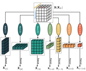
Figure 1: In the case of $N=3$, the acquisition for all ${\bar{\bm{\mathsfit{X}}}}_{\mathcal{P}},\ {\mathcal{P}}\subseteq{\mathcal{N}}$.

Furthermore, we analyze the changes in computational complexity and the number of parameters brought about by this degeneration. In (16), for ${\rm FC}(\cdot)$, the number of multiplications is $\mathcal{O}({\bar{M}}^{2}D_{\rm I}D_{\rm O})$, and the number of parameters is $\mathcal{O}({\bar{M}}^{2}D_{\rm I}D_{\rm O})$. For ${\rm FC}_{\rm PE}(\cdot)$, since the power set of ${\mathcal{N}}$ consists of $2^{N}$ elements, the computational complexity and the number of parameters are ${\mathcal{O}}(2^{N}{\bar{M}}D_{\rm I}D_{\rm O})$ and ${\mathcal{O}}(2^{N}D_{\rm I}D_{\rm O})$, respectively. Given ${\bar{M}}=\Pi^{N}_{n=1}M_{n}$, it holds that ${\bar{M}}\gg 2^{N}$ when $M_{n}>2,n\in{\mathcal{N}}$, which means ${\rm FC}_{\rm PE}(\cdot)$ significantly reduces the complexity. Note that the computational complexity of ${\rm FC}(\cdot)$ is determined by ${\bar{M}}^{2}$, while that of ${\rm FC}_{\rm PE}(\cdot)$ is only determined by ${\bar{M}}$. Furthermore, the number of parameters in ${\rm FC}(\cdot)$ is dependent on ${\bar{M}}$, while that of ${\rm FC}_{\rm PE}(\cdot)$ is solely determined by $N$. Additionally, the computational complexity of the multiplication operation between a $2^{N}$ tensor in (17) and matrices becomes high when $N$ is large. To prioritize performance over excessive loss, when constructing the network, selecting a specific part of matrices from the $2^{N}$ matrices ${\bf W}_{{\mathcal{P}}}$ and setting the remaining ones to zero matrices can reduce the complexity.

III-B High-Order Equivariant Module

In this subsection, we construct functions satisfying high-order equivariance. Taking the $1$-$2$-order equivariance in (11b) as an example, we try to find functions $f:\mathbb{R}^{M\times D_{\rm I}}\to\mathbb{R}^{M\times M\times D_{\rm O}}$ satisfying

$$f({\pi_{M}}\circ{\bf X})=\pi_{M}\circ_{[1,2]}f({\bf X}),\ \forall{\pi}_{M}\in{\mathbb{S}}_{M},$$ (18)

where ${\bf X}\in\mathbb{R}^{M\times D_{\rm I}}$ is the input. Similar to (16), we define the FC layer ${\bm{\mathsfit{Y}}}={\rm FC}({\bf X})={\rm vec}^{-1}\left({\bf W}{\rm vec}({\bf X})+{\bf b}\right)$, where ${\bf W}\in\mathbb{R}^{MD_{\rm I}\times M^{2}D_{\rm O}}$ denotes the weight, ${\bf b}\in\mathbb{R}^{M^{2}D_{\rm O}\times 1}$ denotes the bias.

Proposition 5.

Any FC layer ${\bm{\mathsfit{Y}}}={\rm FC}({\bm{\mathsfit{X}}})$ satisfying the $1$-$2$-order equivariance (18) can be represented as

$${\rm FC}_{\rm HOE}({\bf X})=\sum_{i=1}^{5}\left({{\bm{\mathsfit{X}}}}_{i}\times\!{\bf W}_{i}\right)+{\bf 1}\!\otimes_{2}\!{\bf b}^{T}_{\rm HOE},$$ (19)

where ${\bf W}_{i}\in\mathbb{R}^{D_{\rm I}\times D_{\rm O}}$ is the learnable matrix for ${{\bm{\mathsfit{X}}}}_{i}$, and ${\bf b}_{\rm PE}\in\mathbb{R}^{D_{\rm O}\times 1}$ denotes the bias. The expression of ${{\bm{\mathsfit{X}}}}_{i}$ is given by

$${\bm{\mathsfit{X}}}_{1}=({\bf 1}_{1\times 1\times D_{\rm I}}\otimes_{1}{\bf I}_{M})\odot{\bf X},$$ (20)

$${\bm{\mathsfit{X}}}_{2}={\bf 1}_{M\times M\times D_{\rm I}}\odot{\bf X},$$ (21)

$${\bm{\mathsfit{X}}}_{3}=({\bf 1}_{M\times M\times D_{\rm I}}\odot{\bf X})^{T(1,2)},$$ (22)

$${\bm{\mathsfit{X}}}_{4}=({\bf 1}_{1\times 1\times D_{\rm I}}\otimes_{1}{\bf I}_{M})\odot{\bar{\bf X}}_{\{1\}},$$ (23)

$${\bm{\mathsfit{X}}}_{5}={\bf 1}_{M\times M\times D_{\rm I}}\odot{\bar{\bf X}}_{\{1\}},$$ (24)

where $T(1,2)$ represents the transpose of the tensor over the first two dimensions.

The proposition can be demonstrated similarly to Proposition 4 based on [48] and [49]. The computational complexity and parameter count of ${\rm FC}(\cdot)$ are ${\mathcal{O}}(M^{3}D_{\rm I}^{2}D_{\rm O})$ and ${\mathcal{O}}(M^{3}D_{\rm I}^{2}D_{\rm O})$, respectively, while those of ${\rm FC}_{\rm HOE}(\cdot)$ are ${\mathcal{O}}(M^{2}D_{\rm I}^{2}D_{\rm O})$ and ${\mathcal{O}}(D_{\rm I}D_{\rm O})$, respectively. When applied to tensors, one can only do the operation for certain two dimensions and regard the other dimensions as batch dimensions. For example, when we apply ${\rm FC}_{\rm HOE}(\cdot)$ to the last two dimensions of ${\bm{\mathsfit{X}}}\in\mathbb{R}^{M_{1}\times\cdots\times M_{N}\times D_{\rm I}}$, for all $m_{1}\in\{1,...,M_{1}\}$,…, $m_{N-1}\in\{1,...,M_{N-1}\}$, execute the following same operation

$${{\bm{\mathsfit{Y}}}}_{[m_{1},...,m_{N-1},:]}={\rm FC}_{\rm HOE}({\bm{\mathsfit{X}}}_{[m_{1},...,m_{N-1},:,:]})\in\mathbb{R}^{M_{N}\times M_{N}\times D_{\rm O}}.$$ (25)

The above operation can be executed in parallel through batch computation. Besides, the weights of equivariant modules that satisfy arbitrary orders of equivariance exhibit more intricate patterns, which can be found in [48].

III-C Multi-Dimensional Invariant Module

In this subsection, we develop functions satisfying multidimensional invariance for the mappings like those in (15b) and (15c). The simplest invariant functions include summation, averaging, and maximum operations, i.e., $f_{1}({\bm{\mathsfit{X}}})={\rm Sum}_{\mathcal{N}_{\rm I}}({\bm{\mathsfit{X}}})$, $f_{2}({\bm{\mathsfit{X}}})={\rm Mean}_{\mathcal{N}_{\rm I}}({\bm{\mathsfit{X}}})$, $f_{3}({\bm{\mathsfit{X}}})={\rm Max}_{\mathcal{N}_{\rm I}}({\bm{\mathsfit{X}}})$, where the subscript $\mathcal{N}_{\rm I}$ denotes operations performed across dimensions in $\mathcal{N}_{\rm I}$. Nevertheless, the above invariant functions are all non-parametric and exhibit poor performance. To this end, we introduce the function PMA in [43] for constructing parameterized multidimensional invariant functions. Its expression is as follows

$${\rm PMA}({\bf X})={\rm MAB}({\bf S},{\rm FFC}({\bf X}))\in\mathbb{R}^{J\times D_{\rm O}},$$ (26)

where ${\bf X}\in\mathbb{R}^{M\times D_{\rm I}}$ is the input matrix, and ${\bf S}\in\mathbb{R}^{J\times D_{\rm I}}$ is a learnable parameter matrix, $M$ denotes the number of input items, and $D_{\rm O}$ represents the output feature length. $J$ controls the dimension of the output matrix. Without loss of generality, we all subsequently set $J=1$. The expression of ${\rm MAB}(\cdot)$ is given by

$${\rm MAB}({\bf X}^{\prime},{\bf Y}^{\prime})={\bf M}^{\prime}+{\rm ReLU}\left({\rm FFC}({\bf M}^{\prime})\right),$$ (27)

$${\bf M}^{\prime}={\rm LN}({\bf X}^{\prime}+{\rm MultiHead}({\bf X}^{\prime},{\bf Y}^{\prime},{\bf Y}^{\prime})).$$ (28)

${\rm MultiHead}(\cdot)$ denotes the multi-head attention module [50], whose expression can be written as ${\rm MultiHead}({\bf Q},{\bf K},{\bf V})=[{\rm head}_{1},...,{\rm head}_{N_{\rm H}}]{\bf W}^{O}$, where

$${\rm head}_{i}={\rm Attention}({\bf Q}{\bf W}^{Q}_{i},{\bf K}{\bf W}^{K}_{i},{\bf V}{\bf W}^{V}_{i}),$$ (29)

where ${\bf W}^{Q},{\bf W}^{K},{\bf W}^{V}\in{\mathbb{R}}^{D_{\rm I}\times\frac{D_{\rm O}}{N_{\rm H}}}$ and ${\bf W}^{O}\in{\mathbb{R}}^{D_{\rm O}\times{D_{\rm O}}}$ are learnable weights; $N_{\rm H}$ is the number of heads. The ${\rm Attention}(\cdot)$ function is given by

$${\rm Attention}({\bar{\bf Q}},{\bar{\bf K}},{\bar{\bf V}})\!=\!{\rm Softmax}\!\left(\!{{\bar{\bf Q}}{\bar{\bf K}}^{T}}\!/\!{\sqrt{{D_{\rm I}}/{N_{\rm H}}}}\right)\!{\bar{\bf V}},$$ (30)

where ${\rm Softmax}$ is performed at the second dimension. In summary, the process of ${\rm PMA}(\cdot)$ are given by (26)-(30).

It is easy to prove that the parameterized invariant function ${\rm PMA}:\mathbb{R}^{M\times D_{\rm I}}\to\mathbb{R}^{1\times D_{\rm O}}$ satisfies the invariance. Similar to ${\rm FC}_{\rm HOE}(\cdot)$, ${\rm PMA}(\cdot)$ can be applied to a single dimension of a tensor with batch computation. Applying ${\rm PMA}(\cdot)$ separately to multiple dimensions can achieve multidimensional invariance. The computational complexity of ${\rm PMA}(\cdot)$ mainly resides in (27)-(30), denoted as ${\mathcal{O}}({\bar{M}}D_{\rm O}(D_{\rm I}+D_{\rm O}))$, with the number of parameters ${\mathcal{O}}(D_{\rm O}(D_{\rm I}+D_{\rm O}))$.

III-D Advantages of TENN Modules

The TENN modules designed in Sections III-A-III-C satisfy TE that aligns with mappings mentioned in Section II. Considering conventional NNs can approximate almost any mapping [10], a natural question arises: Why should we exploit TE for NN design? Based on the analysis in Sections III-A-III-C, we provide several reasons as follows:

• Parameter sharing: The TENN modules lead to specific parameter sharing patterns [41, 29], greatly reducing the number of parameter. Furthermore, the parameter count is independent of input size, which provides advantages for scenarios that involve a large number of items [51].

• Lower complexity: The reduction in the number of parameters further leads to a decrease in computational complexity [41]. As the input size increases, the rate of complexity growth is relatively slow.

• Flexible input size: Since the parameters of equivariant networks are independent of the number of inputs, the network can work in scenarios with different input sizes without any modification [28, 48].

• Widespread presence: It is easily demonstrated that the design of modulation [52], soft demodulation [40], detection [39], channel estimation [53] (or other parameter estimation), and other aspects also involve TE. Moreover, the dimensionality of these properties grows with the increases of device types in the system, such as access points, reconfigurable intelligent surfaces, and unmanned aerial vehicles.

IV Tensor Equivariance Framework
for NN Design

In this section, by leveraging the plug-and-play TENN modules, we first present the TE framework for NN design. Based on this framework, we construct NNs for solving optimization problems outlined in Section II, as exemplified.

IV-A Unified TE Framework

Firstly, we present the following proposition to establish the foundation for stacking equivariant layers, thus achieving different TE in certain dimensions.

Proposition 6.

The high-order equivariant layers and multidimensional invariant layers retain their properties when stacked with high-dimensional equivariant layers in front of them.

As this proposition can be readily proven [43], its proof is omitted here. Building upon this proposition, we propose the following design framework.

1. Find TE: Similar to Section II-B, by comparing the dimensions of available and required tensors, seeking equivariance in the process of solving optimization problems.

2. Construct ${\bm{\mathsfit{X}}}$ and ${\bm{\mathsfit{Y}}}$: Given the properties to be satisfied in each dimension, available tensors are manipulated through operations such as repetition and concatenation to construct the input ${\bm{\mathsfit{X}}}$ of the network. Similarly, the desired output ${\bm{\mathsfit{Y}}}$ is constructed for the required tensors.

3. Bulid equivariant network: Based on the TE required by the mapping from ${\bm{\mathsfit{X}}}$ to ${\bm{\mathsfit{Y}}}$, select modules from those proposed in Section II, and then stack them to form the equivariant NN.

4. Design the output layer: The schemes in wireless communication system are usually constrained by various limitations, such as the transmit power. Therefore, it is necessary to design the output layer of the network to ensure that the outputs satisfy the constraints.

It is noteworthy that most of the existing techniques applicable to the design of AI-assisted communication schemes remain relevant within this framework. For instance, the technique of finding low-dimensional variables in [18], the approach for non-convex optimization problems presented in [26], and the residual connection for deep NNs in [54].

IV-B TENN Design for Precoding

Compared to the precoding tensor ${\bm{\mathsfit{W}}}$, the auxiliary tensors ${\bm{\mathsfit{A}}}^{\star},{\bm{\mathsfit{U}}}^{\star}$ in the optimal closed-form expression have smaller size, and incorporating such expression as the model-driven component can reduce the difficulty of NN training. Therefore, in this section, we consider designing NN to approximate the mapping from ${\bm{\mathsfit{H}}},\sigma^{2}$ to ${\bm{\mathsfit{A}}}^{\star},{\bm{\mathsfit{U}}}^{\star}$.

IV-B1 Find TE

According to Section II-B, the mapping satisfys the equivariance in (11a)-(11c).

IV-B2 Construct The Input and Output

We construct the input and output of the TENN as follows

$${\bm{\mathsfit{X}}}\!=\![\real({\bm{\mathsfit{H}}}),\Im({\bm{\mathsfit{H}}}),\sigma^{2}{\bf 1}]_{4}\!\in\!\mathbb{R}^{K\times N_{\rm R}\times N_{\rm T}\times D_{X}},$$ (31)

$${\bm{\mathsfit{Y}}}\!=\![\real({\bm{\mathsfit{A}}}^{\star}),\!\Im({\bm{\mathsfit{A}}}^{\star}),\!\real({\bm{\mathsfit{U}}}^{\star}),\Im({\bm{\mathsfit{U}}}^{\star})]_{4}\!\in\!\mathbb{R}^{K\times N_{\rm R}\times N_{\rm R}\times D_{Y}},$$ (32)

where $D_{X}=3$ and $D_{Y}=4$. The mapping $G(\cdot)$ from ${\bm{\mathsfit{X}}}$ to ${\bm{\mathsfit{Y}}}$ satisfies the following properties

$$G({\pi_{K}}\!\circ_{1}\!{\bm{\mathsfit{X}}})=\pi_{K}\circ_{1}{\bm{\mathsfit{Y}}},\ \forall{\pi}_{K}\in{\mathbb{S}}_{K},$$ (33)

$$G({\pi_{N_{\rm R}}}\!\circ_{2}{\bm{\mathsfit{X}}})=\pi_{N_{\rm R}}\circ_{[2,3]}{\bm{\mathsfit{Y}}},\ \forall{\pi}_{N_{\rm R}}\in{\mathbb{S}}_{N_{\rm R}},$$ (34)

$$G({\pi_{N_{\rm T}}}\!\circ_{3}{\bm{\mathsfit{X}}})={\bm{\mathsfit{Y}}},\ \forall{\pi}_{N_{\rm T}}\in{\mathbb{S}}_{N_{\rm T}}.$$ (35)

IV-B3 Bulid Equivariant Network

The constructed network is illustrated in Fig. 2. We first use the ${\rm FFC}_{1}(\cdot)$ to elevate the feature length of ${\bm{\mathsfit{X}}}$ from $D_{X}$ to the hidden layer feature length $D_{\rm H}$. Since the desired function $G(\cdot)$ exhibits equivariance in the first three dimensions of ${\bm{\mathsfit{X}}}$, we employ $L$ multidimensional ($N=3$) equivariant module ${\rm FC}_{\rm PE}(\cdot)$ from Section III-A to perform the interaction between features of ${\bm{\mathsfit{X}}}$. Furthermore, considering the invariance of $G(\cdot)$ in (35), we employ the module ${\rm PMA}(\cdot)$ from Section III-C, which satisfies the invariance, on the third dimension. Additionally, to satisfy the high-order equivariance in (34), we apply the high-order equivariant module ${\rm FC}_{\rm HOE}(\cdot)$ from Section III-B on the second dimension. $D_{\rm I}$ and $D_{\rm O}$ of all mentioned equivariant modules are equal to $D_{\rm H}$. Finally, we employ ${\rm FFC}_{2}(\cdot)$ to reduce the feature length from $D_{\rm H}$ to $D_{\rm Y}$. Between modules, we incorporate ReLU for element-wise nonlinearity, and adopt layer normalization (LN) to expedite training and improve performance [55]. We refer to this network used for precoding as ‘TEPN’.

Figure 2: The architecture of TEPN.

IV-B4 Design The Output Layer

${\bm{\mathsfit{A}}}$ and ${\bm{\mathsfit{U}}}$ are key variables in the closed-form precoding expression, with constraints not explicitly shown. Therefore, the operations at the output layer are as follows

$${\bm{\mathsfit{A}}}={\bm{\mathsfit{Y}}}_{[:,:,:,1]}+j{\bm{\mathsfit{Y}}}_{[:,:,:,2]},\ {\bm{\mathsfit{U}}}={\bm{\mathsfit{Y}}}_{[:,:,:,3]}+j{\bm{\mathsfit{Y}}}_{[:,:,:,4]}.$$ (36)

By combining the decomposition of tensors into matrices and the concatenation of matrices into tensors, we can compute the final precoding scheme ${\hat{\bm{\mathsfit{W}}}}$ from ${\bm{\mathsfit{A}}}$ and ${\bm{\mathsfit{U}}}$ using (6).

Given the optimization problem (4) for precoding, we employ unsupervised learning, with the negative loss function chosen as the objective function of problem (4), i.e.,

$${\rm Loss}=-\frac{1}{N_{\rm sp}}\sum_{n=1}^{N_{\rm sp}}\sum_{k=1}^{K}R_{k}({\bm{\mathsfit{H}}}[n],{\hat{\bm{\mathsfit{W}}}}[n],\sigma^{2}[n]),$$ (37)

where the subscript $[n]$ denotes the $n$-th sample in the dataset, and $N_{\rm sp}$ represents the number of samples.

IV-C TENN Design for User Scheduling

IV-C1 Find TE

According to Section II-B, the design of the user scheduling scheme targets to find the mapping from ${\tilde{{\bm{\mathsfit{H}}}}},\sigma^{2}$ to ${\bm{\eta}}^{\star}$, which satisfys the equivariance in (15a)-(15c).

IV-C2 Construct The Input and Output

We construct the input and output as follows

$${\bm{\mathsfit{X}}}=[\real({\tilde{{\bm{\mathsfit{H}}}}}),\Im({\tilde{{\bm{\mathsfit{H}}}}}),\sigma^{2}{\bf 1}]_{4}\in\mathbb{R}^{{\tilde{K}}\times N_{\rm R}\times N_{\rm T}\times D_{X}},$$ (38)

$${\bf y}={\bm{\eta}}^{\star}\in\mathbb{R}^{{\tilde{K}}\times D_{Y}},$$ (39)

where $D_{X}=3$ and $D_{Y}=1$. The mapping $G(\cdot)$ from ${\bm{\mathsfit{X}}}$ to ${\bf y}$ satisfies the following properties

$$G({\pi_{{\tilde{K}}}}\!\circ_{1}\!{\bm{\mathsfit{X}}})=\pi_{{\tilde{K}}}\circ_{1}{\bf y},\ \forall{\pi}_{{\tilde{K}}}\in{\mathbb{S}}_{{\tilde{K}}},$$ (40)

$$G({\pi_{N_{\rm R}}}\!\circ_{2}{\bm{\mathsfit{X}}})={\bf y},\ \forall{\pi}_{N_{\rm R}}\in{\mathbb{S}}_{N_{\rm R}},$$ (41)

$$G({\pi_{N_{\rm T}}}\!\circ_{3}{\bm{\mathsfit{X}}})={\bf y},\ \forall{\pi}_{N_{\rm T}}\in{\mathbb{S}}_{N_{\rm T}}.$$ (42)

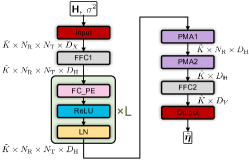
Figure 3: The architecture of TEUSN.

IV-C3 Bulid Equivariant Network

The constructed network is illustrated in Fig. 3. The overall structure is similar to TEPN. The difference lies in replacing ${\rm FC}_{\rm HOE}(\cdot)$ with another ${\rm PMA}(\cdot)$ to satisfy invariance in the second and third dimensions of ${\bm{\mathsfit{X}}}$. We refer to this network used for user scheduling as ‘TEUSN’.

IV-C4 Design The Output Layer

In problem (12), ${\bm{\eta}}$ is constrained as a binary variable with all elements summing up to $K$. To address this, we first employ ${\rm Softmax}(\cdot)$ to transform the output ${\bm{\mathsfit{Y}}}$ into probabilities between 0 and 1, i.e., ${\bm{\eta}}^{\rm pro}={\rm Softmax}({\bf y})$. Subsequently, the largest $K$ elements are set to 1, while the rest are set to 0, which is further denoted by ${\hat{\bm{\eta}}}$.

We employ supervised learning, utilizing the following binary cross-entropy loss for training

$${\rm Loss}=\!-\!\frac{1}{N_{\rm sp}{\tilde{K}}}\sum_{n=1}^{N_{\rm sp}}\sum_{k=1}^{\tilde{K}}{\rm BCE}(\eta^{\rm pro}_{k}[n],\eta^{\star}_{k}[n]),$$ (43)

where ${\bm{\eta}}^{\star}$ is the target result, and ${\rm BCE}(a,b)=a\log(b)+(1-a)\log(1-b)$.

V Numerical Results

In this section, we employ the Monte Carlo method to assess the performance of the proposed methods. We consider a massive MIMO system and utilize QuaDRiGa channel simulator to generate all channel data [56]. The configuration details of the channel model are as follows: The BS is equipped with uniform planar array (UPA) comprising $N_{\rm Tv}=2$ dual-polarized antennas in each column and $N_{\rm Th}$ dual-polarized antennas in each row with the number of antennas $N_{\rm T}=2N_{\rm Tv}N_{\rm Th}$. UEs are equipped with uniform linear array comprising $N_{\rm Rv}=1$ antennas in each column and $N_{\rm Rh}$ antennas in each row with the number of antennas $N_{\rm R}=N_{\rm Rv}N_{\rm Rh}$. In this section, parameters $N_{\rm Th}$ and $N_{\rm Rh}$ are adjusted to accommodate the desired antenna quantity configuration. Both the BS and UEs employ antenna type ‘3gpp-3d’, the center frequency is set at 3.5 GHz, and the scenario is ‘3GPP_38.901_UMa_NLOS’ [57]. Shadow fading and path loss are not considered. The cell radius is 500 meters, with users distributed within a 120-degree sector facing the UPA (3-sector cell). For the convenience of comparison, we consider the normalized channel satisfying $\sum_{k=1}^{K}{\rm Tr}\{{\bf H}_{k}{\bf H}^{H}_{k}\}=KN_{\rm R}N_{\rm T}$ and ${\rm SNR}=P_{\rm T}/{\sigma^{2}}$ [58]. Under the same channel model configuration, all channel realizations are independently generated, implying diversity in the channel environments and terminal locations.

V-A Training Details

For the network TEPN constructed for precoding in Section IV-B, its channel dataset size is $[60000,K,N_{\rm R},N_{\rm T},2]$, with $55000$ channels used for training and $5000$ channels used for testing, and the channels are stored as real and imaginary parts. Similarly, for the network TEUSN constructed for user scheduling in Section IV-C, its channel dataset size is $[60000,{\tilde{K}},N_{\rm R},N_{\rm T},2]$. Besides the label (${\bm{\eta}}^{\star}$) dataset size is $[60000,{\tilde{K}},1]$, where ${\bm{\eta}}^{\star}$ is generated by well-performing conventional scheduling algorithms, as will be discussed in subsequent sections. We employ the same training strategy for TEPN and TEUSN. The number of iterations and batch size are set to be $2\times 10^{5}$ and 2000. We utilize the Adam optimizer with a learning rate of $5\times 10^{-4}$ for the first half of training and $5\times 10^{-5}$ for the latter half [59]. It should be noted that the networks are trained to work in full SNR ranges, and the training data is not used for performance evaluation.

V-B Performance of Precoding Schemes

This section compares the following methods:

• ‘ZF’ and ‘MMSE’: Conventional closed-form linear precoding methods [60].

• ‘WMMSE-RandInt’ and ‘WMMSE-MMSEInit’: Conventional algorithms for iterative solving of the sum-rate maximization precoding problem [4]. WMMSE-RandInt and WMMSE-MMSEInit apply random tensor and MMSE precoding as initial values, respectively. We set the maximum number of iterations to 300 and define the stopping criterion as a reduction in the sum-rate per single iteration being less than $10^{-4}$.

• ‘GNN’: The AI-aided approach utilizing GNN for computation of precoding tensors from CSI [36], where the number of hidden layers is $4$ and the number of hidden layer neurons is $D_{G}=128$.

• ‘TECFP’: The precoding scheme based TEPN in Section IV-B with $L=3$ and $D_{\rm H}=8$.

TABLE I: Computational Complexity of Precoding Schemes

Methods	Complexity Order	Multiplications
ZF	${\mathcal{O}}(N_{\rm T}K^{2}N_{\rm R}^{2})$	$6.1\times 10^{4}$
MMSE	${\mathcal{O}}(N_{\rm T}K^{2}N_{\rm R}^{2})$	$6.1\times 10^{4}$
WMMSE-RandInt	${\mathcal{O}}(T_{\rm P1}N_{\rm T}K^{2}N_{\rm R}^{2})$	$3.0\times 10^{7}$
WMMSE-MMSEInit	${\mathcal{O}}(T_{\rm P2}N_{\rm T}K^{2}N_{\rm R}^{2})$	$3.1\times 10^{7}$
GNN	${\mathcal{O}}(N_{\rm T}KN_{\rm R}D_{G}^{2})$	$1.4\times 10^{8}$
TECFP	${\mathcal{O}}(N_{\rm T}KN_{\rm R}D_{\rm H}^{2}+N_{\rm T}K^{2}N_{\rm R}^{2})$	$1.0\times 10^{6}$

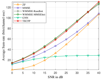
(a) $N_{\rm T}=24$, $K=6$.

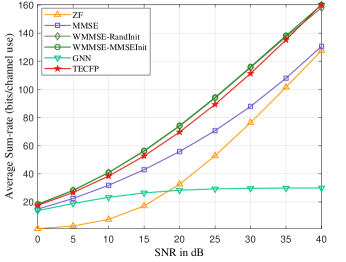
(b) $N_{\rm T}=32$, $K=8$.

Figure 4: Sum rate vs SNR, $N_{\rm R}=2$.

Table I contrasts the computational complexities of several methods in typical scenarios, where “multiplications” refers to the count of real multiplications, with complex multiplications calculated as three times the real ones. It is noteworthy that in the table, $T_{\rm P1}\approx T_{\rm P2}>D_{\rm G}\gg N_{\rm T}>K\approx D_{\rm H}>N_{\rm R}$. Among the considered methods, the complexity of ZF and MMSE precoding, as closed-form linear precoding methods, is the lowest. Although the computational complexity per single iteration of WMMSE precoding shares the same order as MMSE, achieving optimal performance typically requires multiple iterations, introducing high complexity. Additionally, since MMSE and WMMSE still necessitate matrix inversion, their complexity includes second-order terms with respect to $K$ and $N_{\rm R}$. GNN also exhibit parameter-sharing properties, thus their complexity is solely related to the first order of the channel dimensions. However, due to the high dimensionality of the precoding tensor, the approximation for precoding computations requires a substantial number of neurons $D_{G}$, thus introducing substantial complexity. TECFP leverages TE in mappings from CSI to low-dimensional auxiliary tensors, while enjoying the advantage of complexity being solely related to the first order of the channel size and requiring fewer neurons, thereby significantly reducing complexity. The required number of multiplications also validate the aforementioned analysis.

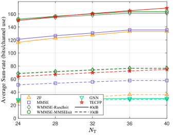
(a) Generalization for different $N_{\rm T}$.

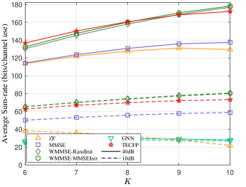
(b) Generalization for different $K$.

Figure 5: Performance generalization of the network trained under scenario $N_{\rm T}=32$, $K=8$, and $N_{\rm R}=2$.

The comparison of sum-rate for each precoding scheme in scenarios $N_{\rm T}=32,K=8,N_{\rm R}=2$ and $N_{\rm T}=24,K=6,N_{\rm R}=2$ is illustrated in Fig. 4. It can be observed that the overall sum-rate performance of precoding schemes with lower computational complexity, such as ZF and MMSE, is significantly lower than that of WMMSE, validating the superior performance of WMMSE. Despite GNN employing a large number of parameters and computational complexity, their performance remains poor. This is attributed to the necessity of matrix inversion for high-dimensional matrices during the computation of precoding matrices, a task that proves exceedingly challenging for deep NNs [35]. In contrast, our proposed method further exploits the closed-form expression of equivariant properties, enabling the approximation of WMMSE performance while maintaining low computational complexity. Fig. 5 demonstrates the generalization capability of the proposed approach. We train our network in scenario $N_{\rm T}=32,K=8,N_{\rm R}=2$ and directly apply it to various different scenarios. It can be observed that the proposed method exhibits consistently outstanding performance, highlighting its robust practical utility.

TABLE II: Computational Complexity of User Scheduing Schemes

Methods	Complexity Order	Multiplications
MMSE-Rand	${\mathcal{O}}(N_{\rm T}K^{2}N_{\rm R}^{2})$	$6.1\times 10^{4}$
MMSE-Greedy	${\mathcal{O}}(K{\tilde{K}}(N_{\rm T}K^{2}N_{\rm R}^{2}))$	$1.8\times 10^{6}$
MMSE-TEUS	${\mathcal{O}}(N_{\rm T}{\tilde{K}}N_{\rm R}D_{{\rm H}1}^{2}+N_{\rm T}K^{2}N_{\rm R}^{2})$	$1.4\times 10^{6}$
WMMSE-Rand	${\mathcal{O}}(T_{P2}N_{\rm T}K^{2}N_{\rm R}^{2})$	$3.1\times 10^{7}$
WMMSE-Greedy	${\mathcal{O}}(K{\tilde{K}}(T_{P2}N_{\rm T}K^{2}N_{\rm R}^{2}))$	$6.4\times 10^{8}$
WMMSE-TEUS	${\mathcal{O}}(N_{\rm T}{\tilde{K}}N_{\rm R}D_{{\rm H}2}^{2}+T_{P2}N_{\rm T}K^{2}N_{\rm R}^{2})$	$5.8\times 10^{7}$
TECFP-TEUS	${\mathcal{O}}(N_{\rm T}{\tilde{K}}N_{\rm R}D_{{\rm H}2}^{2}+N_{\rm T}K^{2}N_{\rm R}^{2})$	$2.8\times 10^{7}$

V-C Performance of User Scheduling Schemes

Based on precoding schemes MMSE, WMMSE (MMSEInit), and TECFP as a foundation, we compare several user scheduling strategies as follows:

• ‘Rand’: Select $K$ users randomly from ${\tilde{K}}$ users.

• ‘Greedy’: Select users one by one from ${\tilde{K}}$ users based on the criterion of maximizing the sum-rate after precoding for the selected users until reaching $K$ users [3].

• ‘TEUS’: The scheduling strategy based on TEUSN trained with the result of greedy scheduling strategy as the label in Section IV-C.

The scheduling strategies vary among different precoding schemes. It is worth noting that the results of greedy user scheduling vary across different precoding schemes. The number of hidden layers and nodes in the TEUS used for MMSE and WMMSE are respectively denoted as $L=3$, $D_{{\rm H}}=8$ and $L=4$, $D_{{\rm H}}=32$.

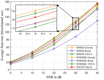
Figure 6: Sum rate vs SNR, $N_{\rm T}=32$, ${\tilde{K}}=12$, $K=8$, $N_{\rm R}=2$.

We compare the computational complexity of several scheduling and precoding combination schemes in Table II. It can be observed that although the greedy scheduling algorithm is designed to select the near-optimal users, it introduces a high computational complexity. The proposed method, TEUS, significantly reduces the overall computational complexity of scheduling and precoding. Specifically, the multiplication count of MMSE-TEUS is approximately 78% of MMSE-Greedy, and that of WMMSE-TEUS is around 9% of WMMSE-Greedy. Furthermore, if the proposed precoding and scheduling schemes are used simultaneously, i.e., employing TECFP-TEUS, the computational complexity will be even lower, potentially below that of WMMSE-Rand, which uses the random scheduling strategy.

Fig. 6 compares the sum-rate performance of various precoding and scheduling combination schemes under scenario $N_{\rm T}=32$, ${\tilde{K}}=12$, $K=8$, $N_{\rm R}=2$. It can be observed that the performance of MMSE-TEUS and WMMSE-TEUS is close to that of MMSE-Greedy and WMMSE-Greedy, respectively. This indicates that the proposed TEUS can achieve outstanding performance at lower computational complexity. Although there is some difference in computational complexity between TECFP-TEUS and WMMSE-Greedy, the former’s computational complexity is even lower, potentially as low as 5% of the latter’s. Furthermore, TECFP-TEUS achieves performance superior to WMMSE-Rand across the entire signal-to-noise ratio range at a lower complexity. Furthermore, in Fig. 7, we compare the generalization ability of the proposed method across different scenarios. We train the TEUS network under scenario $N_{\rm T}=32$, ${\tilde{K}}=12$, $K=8$, $N_{\rm R}=2$ and conduct performance testing under various $N_{\rm T}$ and ${\tilde{K}}$ scenarios. It is evident that, as the scenario changes, the performance trends of MMSE-TEUS, WMMSE-TEUS, and TECFP-TEUS are similar to those of the conventional algorithms MMSE-Greedy and WMMSE-Greedy. This implies that these proposed schemes possess outstanding capability to be directly extended for application in different scenarios.

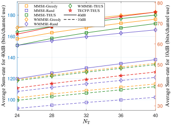
(a) Generalization for different $N_{\rm T}$.

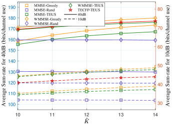
(b) Generalization for different ${\tilde{K}}$.

Figure 7: Performance generalization of the network trained under scenario $N_{\rm T}=32$, $K=8$, and $N_{\rm R}=2$.

VI Conclusion

In this paper, we proposed the unified TE framework, leveraging equivariance in MU-MIMO systems. Firstly, we defined the concept of TE, which encompasses definitions of multiple equivariance properties. On this basis, we put forward the TE framework, which is capable of designing NNs with TE for MU-MIMO systems. In this framework, the various modules are plug-and-play, allowing them to be stacked to accommodate different properties and applicable for various wireless communication tasks. Taking precoding and user scheduling problems as examples, we effortlessly designed corresponding AI-assisted schemes using this framework. The corresponding simulation results validates the superiority of the proposed modules and the unified TE framework.

Appendix A Proof of Proposition 1

We demonstrate partial conclusions in the proposition as follows

$$\sum_{k=1}^{K}R_{k}({\bm{\mathsfit{H}}},{\bm{\mathsfit{W}}},\sigma^{2}) =\sum_{k=1}^{K}R_{k}(\pi_{K}\circ_{1}{\bm{\mathsfit{H}}},\pi_{K}\circ_{1}{\bm{\mathsfit{W}}},\sigma^{2}),$$ (44)

$$=\sum_{k=1}^{K}R_{k}({\pi_{N_{\rm R}}}\!\circ_{2}\!{\bm{\mathsfit{H}}},{\pi_{N_{\rm R}}}\!\circ_{2}\!{\bm{\mathsfit{W}}},\sigma^{2}),$$ (45)

$$=\sum_{k=1}^{K}R_{k}({\pi_{N_{\rm T}}}\!\circ_{3}\!{\bm{\mathsfit{H}}},{\pi_{N_{\rm T}}}\!\circ_{3}\!{\bm{\mathsfit{W}}},\sigma^{2}).$$ (46)

Then, the remaining conclusions in the proposition can be obtained through proof by contradiction.

We first consider the proof of (44). For convenience, we use $\pi$ to denote $\pi_{K}$, and the sum-rate expression considering its influence is as follows

$$\begin{split}&R_{k}(\pi\circ_{1}{\bm{\mathsfit{H}}},\pi\circ_{1}{\bm{\mathsfit{W}}},\sigma^{2})\\ &=\log{\rm det}\left({\bf I}+{\bf W}_{\pi(k)}{\bf H}^{H}_{\pi(k)}({\bm{\Omega}}^{\prime}_{k})^{-1}{\bf H}_{\pi(k)}{\bf W}^{H}_{\pi(k)}\right),\end{split}$$ (47)

where ${\bm{\Omega}}^{\prime}_{k}=\sigma^{2}{\bf I}+\sum_{i=1,i\neq{\pi(k)}}^{K}{\bf H}_{\pi(k)}{\bf W}^{H}_{i}{\bf W}_{i}{\bf H}^{H}_{\pi(k)}={\bm{\Omega}}_{\pi(k)}$. Thus, we have

$$R_{k}(\pi\circ_{1}{\bm{\mathsfit{H}}},\pi\circ_{1}{\bm{\mathsfit{W}}},\sigma^{2})$$

$$=\log{\rm det}\left({\bf I}+{\bf W}_{\pi(k)}{\bf H}^{H}_{\pi(k)}{\bm{\Omega}}^{-1}_{\pi(k)}{\bf H}_{\pi(k)}{\bf W}^{H}_{\pi(k)}\right)$$ (48)

$$=R_{\pi(k)}({\bm{\mathsfit{H}}},{\bm{\mathsfit{W}}},\sigma^{2}).$$

Substituting this expression into (44) yields its validity.

Subsequently, we consider the proof of (45) and use $\pi$ to denote $\pi_{N_{\rm R}}$. We define the permutation matrix ${\bm{\Pi}}$ to represent the permutation of $\pi$ at the second dimension of ${\bm{\mathsfit{H}}}$ and ${\bm{\mathsfit{W}}}$. In matrix ${\bm{\Pi}}$, each row contains only one element equal to 1, with all other elements being 0, and all elements 1 are located in distinct columns. Note that ${\bm{\Pi}}{\bm{\Pi}}^{T}={\bf I}$. For $\pi\circ_{2}{\bm{\mathsfit{H}}}$ and $\pi\circ_{2}{\bm{\mathsfit{W}}}$, the corresponding channel and precoder of the $k$-th user can be expressed as ${\bf H}^{\prime}_{k}={\bm{\Pi}}{\bf H}_{k}$ and ${\bf W}^{\prime}_{k}={\bm{\Pi}}{\bf W}_{k}$. On this basis, we have

$$\begin{split}&R_{k}(\pi\circ_{2}{\bm{\mathsfit{H}}},\pi\circ_{2}{\bm{\mathsfit{W}}},\sigma^{2})\\ &=\log{\rm det}\left({\bf I}+{\bf W}^{\prime}_{k}({\bf H}^{\prime}_{k})^{H}({\bm{\Omega}}^{\prime}_{k})^{-1}{\bf H}^{\prime}_{k}({\bf W}^{\prime}_{k})^{H}\right)\\ &=\log{\rm det}\left({\bf I}+{\bm{\Pi}}{\bf W}_{k}{\bf H}^{H}_{k}{\bm{\Pi}}^{T}({\bm{\Omega}}^{\prime}_{k})^{-1}{\bm{\Pi}}{\bf H}_{k}{\bf W}_{k}^{H}{\bm{\Pi}}^{H}\right),\end{split}$$ (49)

where ${\bm{\Omega}}^{\prime}_{k}=\sigma^{2}{\bf I}+\sum_{i=1,i\neq k}^{K}{\bm{\Pi}}{\bf H}_{k}{\bf W}^{H}_{i}{\bm{\Pi}}^{T}{\bm{\Pi}}{\bf W}_{i}{\bf H}^{H}_{k}{\bm{\Pi}}^{T}$. According to Sylvester determinant identity that $\det({\bf I}+{\bf A}{\bf B})=\det({\bf I}+{\bf B}{\bf A})$, it can be derived that

$$\begin{split}&R_{k}(\pi\circ_{2}{\bm{\mathsfit{H}}},\pi\circ_{2}{\bm{\mathsfit{W}}},\sigma^{2})\\ &=\log{\rm det}\left({\bf I}+{\bf W}_{k}{\bf H}^{H}_{k}{\bm{\Pi}}^{T}({\bm{\Omega}}^{\prime}_{k})^{-1}{\bm{\Pi}}{\bf H}_{k}{\bf W}_{k}^{H}\right).\end{split}$$ (50)

According to Woodbury matrix identity, we have $({\bm{\Omega}}^{\prime}_{k})^{-1}={\bm{\Pi}}({\bm{\Omega}}_{k})^{-1}{\bm{\Pi}}^{T}$. Substituting this expression into (50) yields

$$R_{k}(\pi\circ_{2}{\bm{\mathsfit{H}}},\pi\circ_{2}{\bm{\mathsfit{W}}},\sigma^{2})=R_{k}({\bm{\mathsfit{H}}},{\bm{\mathsfit{W}}},\sigma^{2}).$$ (51)

Therefore, (45) holds.

Finally, we consider the proof of (46). We use $\pi$ to denote $\pi_{N_{\rm T}}$ and utilize ${\bm{\Pi}}$ to represent its permutation. Similar to the last paragraph, we define ${\bf H}^{\prime}_{k}={\bf H}_{k}{\bm{\Pi}}^{T}$ and ${\bf W}^{\prime}_{k}={\bf W}_{k}{\bm{\Pi}}^{T}$. Then, we have

$$\begin{split}&R_{k}(\pi\circ_{3}{\bm{\mathsfit{H}}},\pi\circ_{3}{\bm{\mathsfit{W}}},\sigma^{2})\\ &=\log{\rm det}\left({\bf I}+{\bf W}^{\prime}_{k}({\bf H}^{\prime}_{k})^{H}({\bm{\Omega}}^{\prime}_{k})^{-1}{\bf H}^{\prime}_{k}({\bf W}^{\prime}_{k})^{H}\right)\\ &=\log{\rm det}\left({\bf I}+{\bf W}_{k}{\bf H}^{H}_{k}({\bm{\Omega}}^{\prime}_{k})^{-1}{\bf H}_{k}{\bf W}_{k}^{H}\right),\end{split}$$ (52)

where ${\bm{\Omega}}^{\prime}_{k}\!=\!\sigma^{2}{\bf I}+\sum_{i=1,i\neq k}^{K}{\bf H}_{k}{\bm{\Pi}}^{T}{\bm{\Pi}}{\bf W}^{H}_{i}{\bf W}_{i}{\bm{\Pi}}^{T}{\bm{\Pi}}{\bf H}^{H}_{k}={\bm{\Omega}}_{k}$. Substituting this expression into (52), it is easy to see that (46) holds.

Based on (44)-(46), Given a fixed $\sigma$, it is easy to prove that if ${\bm{\mathsfit{W}}}^{\star}$ is one of the optimal solutions for problem (4) based on ${\bm{\mathsfit{H}}}$, then $\pi_{K}\circ_{1}{\bm{\mathsfit{W}}}^{\star}$, $\pi_{N_{\rm R}}\circ_{2}{\bm{\mathsfit{W}}}^{\star}$, and $\pi_{N_{\rm T}}\circ_{3}{\bm{\mathsfit{W}}}^{\star}$ are also ones of the optimal solutions for problem (4) based on $\pi_{K}\circ_{1}{\bm{\mathsfit{H}}}$, $\pi_{N_{\rm R}}\circ_{2}{\bm{\mathsfit{H}}}$, and $\pi_{N_{\rm T}}\circ_{3}{\bm{\mathsfit{H}}}$, respectively. This completes the proof.

Appendix B Proof of Proposition 2

Based on Proposition 1, the validity of the following equation leads to the establishment of Proposition 2.

$$\pi_{K}\circ_{1}{\bm{\mathsfit{W}}}={\rm CFP}\left(\pi_{K}\!\circ_{1}\!{\bm{\mathsfit{H}}},\pi_{K}\!\circ_{1}\!{\bm{\mathsfit{A}}},\pi_{K}\!\circ_{1}\!{\bm{\mathsfit{U}}},\sigma^{2}\right),$$ (53)

$${\pi_{N_{\rm R}}}\!\circ_{2}\!{\bm{\mathsfit{W}}}\!=\!{\rm CFP}\left({\pi_{N_{\rm R}}}\!\circ_{2}\!{\bm{\mathsfit{H}}},{\pi_{N_{\rm R}}}\!\circ_{[2,3]}\!{\bm{\mathsfit{A}}},{\pi_{N_{\rm R}}}\!\circ_{[2,3]}\!{\bm{\mathsfit{U}}},\sigma^{2}\right),$$ (54)

$${\pi_{N_{\rm T}}}\!\circ_{3}\!{\bm{\mathsfit{W}}}\!=\!{\rm CFP}\left({\pi_{N_{\rm T}}}\!\circ_{3}\!{\bm{\mathsfit{H}}},{\bm{\mathsfit{A}}},{\bm{\mathsfit{U}}},\sigma^{2}\right),$$ (55)

where ${\bm{\mathsfit{W}}}={\rm CFP}\left({\bm{\mathsfit{H}}},{\bm{\mathsfit{A}}},{\bm{\mathsfit{U}}}\right)$. Next, we will separately prove these equations.

We first consider the proof of (53). We use $\pi$ to denote $\pi_{K}$ and define ${\bm{\mathsfit{W}}}^{\prime}={\rm CFP}\left(\pi_{K}\!\circ_{1}\!{\bm{\mathsfit{H}}},\pi_{K}\!\circ_{1}\!{\bm{\mathsfit{A}}},\pi_{K}\!\circ_{1}\!{\bm{\mathsfit{U}}}\right)$. According to (6) and Woodbury matrix identity, we have

$${\tilde{\bf W}}^{\prime}_{k}\!=\!{\bf U}_{\pi(k)}^{T}{\bf A}^{*}_{\pi(k)}{\bf H}^{*}_{\pi(k)}\left({\bm{\Upsilon}}+\mu^{\prime}{\bf I}_{N}\right)^{-1},$$ (56)

where ${\bm{\Upsilon}}=\sum_{k=1}^{K}{\bf H}^{H}_{k}{\bf A}^{H}_{k}{\bf U}_{k}{\bf A}_{k}{\bf H}_{k}$, $\mu^{\prime}={{\rm Tr}\left({\bf U}^{\prime}{\bf A}^{\prime}{\bf A}^{\prime H}\right)}={{\rm Tr}\left({\bf U}{\bf A}{\bf A}^{H}\right)}=\mu$, ${\bf U}^{\prime}={\rm blkdiag}\{{\bf U}_{\pi(1)},...,{\bf U}_{\pi(K)}\}$, and ${\bf A}^{\prime}={\rm blkdiag}\{{\bf A}_{\pi(1)},...,{\bf A}_{\pi(K)}\}$. Then, we can concludes ${\tilde{\bf W}}^{\prime}_{k}={\tilde{\bf W}}_{\pi(k)}$, which leads to ${\bm{\mathsfit{W}}}^{\prime}=\pi_{K}\circ_{1}{\bm{\mathsfit{W}}}$.

Subsequently, we consider the proof of (54). We use $\pi$ to denote $\pi_{N_{\rm R}}$. We define the permutation matrix ${\bm{\Pi}}$ to represent the permutation of $\pi$ at ${\bm{\mathsfit{H}}}$, ${\bm{\mathsfit{A}}}$, and ${\bm{\mathsfit{U}}}$. For $\pi\circ_{2}{\bm{\mathsfit{H}}}$, $\pi\circ_{[2,3]}{\bm{\mathsfit{A}}}$, and $\pi\circ_{[2,3]}{\bm{\mathsfit{U}}}$. The corresponding channel and auxiliary tensors of the $k$-th user can be expressed as ${\bf H}^{\prime}_{k}={\bm{\Pi}}{\bf H}_{k}$, ${\bf A}^{\prime}_{k}={\bm{\Pi}}{\bf A}_{k}{\bm{\Pi}}^{T}$, and ${\bf U}^{\prime}_{k}={\bm{\Pi}}{\bf U}_{k}{\bm{\Pi}}^{T}$. After permutation, the expression for the precoding matrix before scaling for the $k$-th user is given by ${\tilde{\bf W}}^{\prime}_{k}={\bm{\Pi}}{\bf U}_{k}^{T}{\bf A}^{*}_{k}{\bf H}^{*}_{k}\left({\bm{\Upsilon}}+\mu^{\prime}{\bf I}_{N}\right)^{-1}$, which leads to ${\bm{\mathsfit{W}}}^{\prime}={\bm{\Pi}}{\tilde{\bf W}}_{k}=\pi\circ_{2}{\bm{\mathsfit{W}}}$.

Finally, we consider the proof of (55). We use $\pi$ to denote $\pi_{N_{\rm T}}$ and utilize ${\bm{\Pi}}$ to represent its permutation. After permutation, the expression for the precoding matrix before scaling for the $k$-th user is given by

$$\textstyle{\tilde{\bf W}}^{\prime}_{k}$$

$$\textstyle={\bf U}_{k}^{T}{\bf A}^{*}_{k}{\bf H}^{*}_{k}{\bm{\Pi}}^{T}\left(\sum_{k=1}^{K}{\bm{\Pi}}{\bf H}^{H}_{k}{\bf A}^{H}_{k}{\bf U}_{k}{\bf A}_{k}{\bf H}_{k}{\bm{\Pi}}^{T}\!+\!\mu^{\prime}{\bf I}_{N}\right)^{-1}$$

$$\textstyle={\bf U}_{k}^{T}{\bf A}^{*}_{k}{\bf H}^{*}_{k}\left(\sum_{k=1}^{K}{\bf H}^{H}_{k}{\bf A}^{H}_{k}{\bf U}_{k}{\bf A}_{k}{\bf H}_{k}\!+\!\mu^{\prime}{\bf I}_{N}\right)^{-1}{\bm{\Pi}}^{T}.$$

$$\textstyle={\tilde{\bf W}}_{k}{\bm{\Pi}}^{T}.$$ (57)

This equation leads to ${\bm{\mathsfit{W}}}^{\prime}=\pi\circ_{3}{\bm{\mathsfit{W}}}$. This completes the proof.

Appendix C Proof of Proposition 3

Similar to Appendix A, the establishment of Proposition 3 can be proven by demonstrating the validity of the following equations

$$R_{\rm US}({\tilde{\bm{\mathsfit{H}}}},{\bm{\eta}},\sigma^{2})=R_{\rm US}({\pi_{\tilde{K}}}\!\circ_{1}\!{\tilde{\bm{\mathsfit{H}}}},{\pi_{\tilde{K}}}\!\circ_{1}\!{\bm{\eta}},\sigma^{2}),$$ (58)

$$R_{\rm US}({\tilde{\bm{\mathsfit{H}}}},{\bm{\eta}},\sigma^{2})=R_{\rm US}({\pi_{N_{\rm R}}}\!\circ_{2}\!{\tilde{\bm{\mathsfit{H}}}},{\bm{\eta}},\sigma^{2}),$$ (59)

$$R_{\rm US}({\tilde{\bm{\mathsfit{H}}}},{\bm{\eta}},\sigma^{2})=R_{\rm US}({\pi_{N_{\rm T}}}\!\circ_{3}\!{\tilde{\bm{\mathsfit{H}}}},{\bm{\eta}},\sigma^{2}).$$ (60)

For (58), we have

$$R_{\rm US}({\pi}\!\circ_{1}\!{\tilde{\bm{\mathsfit{H}}}},{\pi}\!\circ_{1}\!{\bm{\eta}},\sigma^{2})\!=\!\sum_{k^{\prime}\in{\mathcal{K}}^{\prime}}\!\!\!R_{k^{\prime}}({\bm{\mathsfit{H}}}^{\prime},G_{\rm CP}({\bm{\mathsfit{H}}}^{\prime},\sigma^{2}),\sigma^{2}),$$ (61)

where ${\mathcal{K}}^{\prime}\!=\!\{\pi(k)|\eta_{k}\!=\!1,{k}\!\in\!{{\tilde{\mathcal{K}}}}\}$ and ${\bm{\mathsfit{H}}}^{\prime}=[{\bf H}^{\prime}_{k^{\prime}}]_{0,k^{\prime}\in{\mathcal{K}}^{\prime}}\in\mathbb{C}^{K\times N_{\rm R}\times N_{\rm T}}$. It is easy to verify that ${\bf H}^{\prime}_{k^{\prime}}={\bf H}_{\pi^{-1}(k^{\prime})}$. With the definition of ${\mathcal{K}}^{\prime}$, we can conclude that ${\bm{\mathsfit{H}}}^{\prime}=\pi_{K}\circ_{1}{\bm{\mathsfit{H}}},\pi_{K}\in\mathbb{S}_{K}$. Substituting this equation into (61) yields the establishment of (58).

For (59) and (60), we have

$$R_{\rm US}({\pi_{N_{\rm R}}}\!\circ_{2}\!{\tilde{\bm{\mathsfit{H}}}},{\bm{\eta}},\sigma^{2})\!=\!\sum_{k\in{\mathcal{K}}}R_{k}({\bm{\mathsfit{H}}}^{\prime},G_{\rm CP}({\bm{\mathsfit{H}}}^{\prime},\sigma^{2}),\sigma^{2}),$$ (62)

where ${\bm{\mathsfit{H}}}^{\prime}={\pi_{N_{\rm R}}}\!\circ_{2}\!{\bm{\mathsfit{H}}}$. According to Appendix A, it is straightforward to show that (59) holds. Similarly, it can be proved that (60) also holds. This completes the proof.

Appendix D Proof of Proposition 4

We prove the validity of this proposition under the scenario of $D_{\rm I}=D_{\rm O}=1$, and this conclusion can be easily extended to the scenario of $D_{\rm I}>1$ and $D_{\rm O}>1$. Besides, we temporarily ignore the bias ${\bf b}$ and derive its pattern at the end. We reshape the weights to ${\bm{\mathsfit{W}}}\in\mathbb{R}^{M_{1}\times\cdots\times M_{N}\times M_{1}\times\cdots\times M_{N}}$ and use ${\bm{\mathsfit{W}}}_{[{\bf p},{\bf q}]}$ to represent ${\bm{\mathsfit{W}}}_{[p_{1},...,p_{N},q_{1},...,q_{N}]}$. According to [41], it can be derived that the weights satisfying multidimensional equivariance across dimensions in ${\mathcal{N}}=\{1,...,N\}$ exhibit the following pattern

$${\bm{\mathsfit{W}}}_{[{\bf p},{\bf q}]}\!=\!w_{{\mathcal{P}}}\quad{\rm s.t.}\ p_{i}\!=\!q_{i},\ i\in{{\mathcal{P}}},\ p_{i^{\prime}}\neq q_{i^{\prime}},\ i^{\prime}\in{\mathcal{N}}\backslash{{\mathcal{P}}},$$ (63)

where $w_{{\mathcal{P}}}$ is defined for each ${\mathcal{P}}\subseteq{\mathcal{N}}=\{1,2,...,N\}$. The above equation implies that, for a specific set of dimensions ${\mathcal{P}}$, the elements of ${\bm{\mathsfit{W}}}$, which satisfy that the $N$-dimensional coordinate ${\bf p}$ are the same as the coordinate ${\bf q}$ on dimensions only in ${\mathcal{P}}$, share the same weight $w_{{\mathcal{P}}}$. Due to $|{\mathcal{N}}|=N$, there are $2^{N}$ different elements $w_{{\mathcal{P}}}$ in ${\bm{\mathsfit{W}}}$. Although this pattern is intricate, we will proceed to demonstrate its equivalence to our expression. The $p_{1},...,p_{N}$-th element of ${\bm{\mathsfit{Y}}}$ is given by

$$y_{p_{1},...,p_{N}}$$

$$=\sum_{q_{N}=1}^{M_{N}}\sum_{q_{N-1}=1}^{M_{N-1}}\cdots\sum_{q_{1}=1}^{M_{1}}{\bf W}_{[{\bf p},(q_{1},q_{2},...,q_{N})^{T}]}\cdot x_{q_{1},...,q_{N}}$$

$$=\sum_{{\mathcal{P}}\subseteq{\mathcal{N}}}w_{{\mathcal{P}}}\sum_{q_{i}=p_{i},i\in{\mathcal{P}}\atop q_{i^{\prime}}\neq p_{i^{\prime}},i^{\prime}\in{\mathcal{N}}\backslash{\mathcal{P}}}x_{q_{1},..,q_{N}}$$

$$=w_{\emptyset}\!\!\!\!\sum_{q_{1},...,q_{N}}\!\!\!\!x_{q_{1},q_{2},..,q_{N}}+(w_{\{1\}}\!-\!w_{\emptyset})\!\!\!\!\sum_{q_{2},...,q_{N}}\!\!\!\!x_{p_{1},q_{2},..,q_{N}}+\cdots$$

$$\ \ +(w_{\{N\}}\!-\!w_{\emptyset})\!\!\!\!\sum_{q_{1},...,q_{N-1}}\!\!\!\!x_{q_{1},..,q_{N-1},p_{N}}$$

$$\ \ +\![w_{\{1,2\}}\!-\!(w_{\{1\}}\!-\!w_{\emptyset})\!-\!(w_{\{2\}}\!-\!w_{\emptyset})\!-\!w_{\emptyset}]\!\!\!\!\sum_{q_{3},...,q_{N}}\!\!\!x_{p_{1},p_{2},q_{3},...,q_{N}}$$

$$\ \ +\cdots$$

$$\ \ +(w_{\{1,2,...,N\}}-\cdots-w_{\emptyset})x_{p_{1},...,p_{N}}$$

$$=\sum_{{\mathcal{P}}\subseteq{\mathcal{N}}}{\hat{w}}_{{\mathcal{P}}}\sum_{q_{i}=p_{i},i\in{\mathcal{P}}\atop q_{i^{\prime}},i^{\prime}\in{\mathcal{N}}\backslash{\mathcal{P}}}x_{q_{1},..,q_{N}},$$ (64)

where ${\hat{w}}_{\emptyset}=w_{\emptyset}$ and ${\hat{w}}_{{\mathcal{P}}}=w_{{\mathcal{P}}}-\sum_{{\mathcal{U}}\subset{\mathcal{P}}}{\hat{w}}_{{\mathcal{U}}}$. We use ${\hat{\bm{\mathsfit{X}}}}_{{\mathcal{A}}}\in{\mathbb{R}}^{M_{1}\times\cdots\times M_{N}},{\mathcal{A}}\subseteq{\mathcal{N}}$ to represent the tensor obtained by applying the summation operation over the dimensions ${\mathcal{A}}$ of tensor ${\bm{\mathsfit{X}}}$, which is repeated over the dimensions ${\mathcal{A}}$ to match the original shape. Note that ${\hat{\bm{\mathsfit{X}}}}_{\emptyset}={\bm{\mathsfit{X}}}$. A single term in the above formula can be represented as follows

$$\begin{split}{\hat{w}}_{{\mathcal{P}}}\sum_{q_{i}=p_{i},i\in{\mathcal{P}}\atop q_{i}^{\prime},i^{\prime}\in{\mathcal{N}}\backslash{\mathcal{P}}}\!\!\!x_{q_{1},..,q_{N}}={\hat{w}}_{{\mathcal{P}}}{\hat{\bm{\mathsfit{X}}}}_{{\mathcal{N}}\backslash{\mathcal{P}}[p_{1},p_{2},...,p_{N}]},\end{split}$$ (65)

Based on the above formula, we have $y_{p_{1},...,p_{N}}=\sum_{{\mathcal{P}}\subseteq{\mathcal{N}}}{\hat{w}}_{{\mathcal{P}}}{\hat{\bm{\mathsfit{X}}}}_{{\mathcal{N}}\backslash{\mathcal{P}}[p_{1},p_{2},...,p_{N}]}$. Thus, ${\rm FC}_{\rm PE}({\bm{\mathsfit{X}}})$ can be expressed as

$$\begin{split}&\textstyle{\rm FC}_{\rm PE}({\bm{\mathsfit{X}}})=\sum_{{\mathcal{P}}\subseteq{\mathcal{N}}}{\hat{w}}_{{\mathcal{P}}}{\hat{\bm{\mathsfit{X}}}}_{{\mathcal{N}}\backslash{\mathcal{P}}}=\sum_{{\mathcal{P}}\subseteq{\mathcal{N}}}{\hat{w}}_{{\mathcal{N}}\backslash{\mathcal{P}}}{\hat{\bm{\mathsfit{X}}}}_{{\mathcal{P}}}\\ &\quad=\sum_{{\mathcal{P}}\subseteq{\mathcal{N}}}(\Pi_{n\in{\mathcal{P}}}M_{n})\cdot{\hat{w}}_{{\mathcal{N}}\backslash{\mathcal{P}}}{\bar{\bm{\mathsfit{X}}}}_{{\mathcal{P}}}=\sum_{{\mathcal{P}}\subseteq{\mathcal{N}}}{\bar{w}}_{{\mathcal{P}}}{\bar{\bm{\mathsfit{X}}}}_{{\mathcal{P}}},\end{split}$$ (66)

where ${\bar{w}}_{{\mathcal{P}}}=(\Pi_{n\in{\mathcal{P}}}M_{n})\cdot{\hat{w}}_{{\mathcal{N}}\backslash{\mathcal{P}}}$.

Subsequently, we consider the case where bias exists. We reshape the bias to ${\bm{\mathsfit{B}}}\in\mathbb{R}^{M_{1}\times\cdots\times M_{N}}$. When the elements in ${\bm{\mathsfit{X}}}$ are all zero, (1) degenerates to

$$\textstyle{{\bm{\mathsfit{B}}}=\pi_{M_{n}}\circ_{n}{\bm{\mathsfit{B}}},\ \forall{\pi}_{M_{n}}\in{\mathbb{S}}_{M_{n}},\ \forall n\in\mathcal{N},}$$ (67)

which implies that ${\bm{\mathsfit{B}}}=b{\bf 1}$. Therefore, ${\rm FC}_{\rm PE}({\bm{\mathsfit{X}}})$ can be formulated as $\textstyle{{\rm FC}_{\rm PE}({\bm{\mathsfit{X}}})=\sum_{{\mathcal{P}}\subseteq{\mathcal{N}}}{\bar{w}}_{{\mathcal{P}}}{\bar{\bm{\mathsfit{X}}}}_{{\mathcal{P}}}+b{\bf 1}}$. This expression can be readily extended to scenarios where $D_{\rm I}>1$ and $D_{\rm O}>1$. This completes the proof.

References

- [1] F. Rusek, D. Persson, B. K. Lau, E. G. Larsson, T. L. Marzetta, O. Edfors, and F. Tufvesson, “Scaling up MIMO: Opportunities and challenges with very large arrays,” IEEE Signal Process. Mag., vol. 30, no. 1, pp. 40–60, Jan. 2013.
- [2] C.-X. Wang, X. You, X. Gao, X. Zhu, Z. Li, C. Zhang, H. Wang, Y. Huang, Y. Chen, H. Haas et al., “On the road to 6G: Visions, requirements, key technologies and testbeds,” IEEE Commun. Surv. Tutor., vol. 25, no. 2, pp. 905–974, Secondquarter 2023.
- [3] G. Dimic and N. D. Sidiropoulos, “On downlink beamforming with greedy user selection: Performance analysis and a simple new algorithm,” IEEE Trans. Signal Process., vol. 53, no. 10, pp. 3857–3868, Sept. 2005.
- [4] S. S. Christensen, R. Agarwal, E. De Carvalho, and J. M. Cioffi, “Weighted sum-rate maximization using weighted MMSE for MIMO-BC beamforming design,” IEEE Trans. Wireless Commun., vol. 7, no. 12, pp. 4792–4799, Dec. 2008.
- [5] Q. Shi, M. Razaviyayn, Z.-Q. Luo, and C. He, “An iteratively weighted MMSE approach to distributed sum-utility maximization for a MIMO interfering broadcast channel,” IEEE Trans. Signal Process., vol. 59, no. 9, pp. 4331–4340, Sept. 2011.
- [6] X. Zhao, S. Lu, Q. Shi, and Z.-Q. Luo, “Rethinking WMMSE: Can its complexity scale linearly with the number of BS antennas?” IEEE Trans. Signal Process., vol. 71, pp. 433–446, Feb. 2023.
- [7] B. Hochwald, C. Peel, and A. Swindlehurst, “A vector-perturbation technique for near-capacity multiantenna multiuser communication-Part II: Perturbation,” IEEE Trans. Commun., vol. 53, no. 3, pp. 537–544, 2005.
- [8] M. Costa, “Writing on dirty paper (corresp.),” IEEE Trans. Inf. Theory, vol. 29, no. 3, pp. 439–441, 1983.
- [9] L. Liu and W. Yu, “Massive connectivity with massive MIMO—Part I: Device activity detection and channel estimation,” IEEE Trans. Signal Process., vol. 66, no. 11, pp. 2933–2946, 2018.
- [10] K. Hornik, M. Stinchcombe, and H. White, “Multilayer feedforward networks are universal approximators,” Neural networks, vol. 2, no. 5, pp. 359–366, 1989.
- [11] C. Yun, S. Bhojanapalli, A. S. Rawat, S. J. Reddi, and S. Kumar, “Are transformers universal approximators of sequence-to-sequence functions?” arXiv preprint arXiv:1912.10077, 2019. [Online]. Available: https://arxiv.org/abs/1912.10077
- [12] K. B. Letaief, W. Chen, Y. Shi, J. Zhang, and Y.-J. A. Zhang, “The roadmap to 6G: AI empowered wireless networks,” IEEE Commun. Mag., vol. 57, no. 8, pp. 84–90, Aug. 2019.
- [13] J. Kim, H. Lee, S.-E. Hong, and S.-H. Park, “Deep learning methods for universal MISO beamforming,” IEEE Wireless Commun. Lett., vol. 9, no. 11, pp. 1894–1898, Nov. 2020.
- [14] H. Huang, Y. Peng, J. Yang, W. Xia, and G. Gui, “Fast beamforming design via deep learning,” IEEE Trans. Veh. Technol., vol. 69, no. 1, pp. 1065–1069, Jan. 2019.
- [15] S. Lu, S. Zhao, and Q. Shi, “Learning-based massive beamforming,” in IEEE Glob. Commun. Conf., (GLOBECOM), Dec. 2020, pp. 1–6.
- [16] W. Xia, G. Zheng, Y. Zhu, J. Zhang, J. Wang, and A. P. Petropulu, “A deep learning framework for optimization of MISO downlink beamforming,” IEEE Trans. Commun., vol. 68, no. 3, pp. 1866–1880, Mar. 2020.
- [17] J. Shi, W. Wang, X. Yi, X. Gao, and G. Y. Li, “Deep learning-based robust precoding for massive MIMO,” IEEE Trans. Commun., vol. 69, no. 11, pp. 7429–7443, Nov. 2021.
- [18] J. Shi, A.-A. Lu, W. Zhong, X. Gao, and G. Y. Li, “Robust WMMSE precoder with deep learning design for massive MIMO,” IEEE Trans. Commun., vol. 71, no. 7, pp. 3963–3976, Jul. 2023.
- [19] E. Björnson, M. Bengtsson, and B. Ottersten, “Optimal multiuser transmit beamforming: A difficult problem with a simple solution structure [lecture notes],” IEEE Signal Process. Mag., vol. 31, no. 4, pp. 142–148, Jul. 2014.
- [20] L. Pellaco, M. Bengtsson, and J. Jaldén, “Matrix-inverse-free deep unfolding of the weighted MMSE beamforming algorithm,” IEEE Open J. Commun. Soc., vol. 3, pp. 65–81, Dec. 2021.
- [21] Q. Hu, Y. Cai, Q. Shi, K. Xu, G. Yu, and Z. Ding, “Iterative algorithm induced deep-unfolding neural networks: Precoding design for multiuser MIMO systems,” IEEE Trans. Wireless Commun., vol. 20, no. 2, pp. 1394–1410, Feb. 2021.
- [22] K. Wang and A. Liu, “Robust WMMSE-based precoder with practice-oriented design for massive MU-MIMO,” IEEE Wireless Commun. Lett., Early Access, 2024.
- [23] F. Liang, C. Shen, W. Yu, and F. Wu, “Towards optimal power control via ensembling deep neural networks,” IEEE Trans. Commun., vol. 68, no. 3, pp. 1760–1776, Mar. 2020.
- [24] Y. Li, S. Han, and C. Yang, “User scheduling for uplink OFDMA systems by deep learning,” in IEEE Wireless Commun. Networking Conf. (WCNC), Nanjing, China, Mar. 2020, pp. 1–6.
- [25] B. Xie, S. Chen, S. Zhou, Z. Niu, B. Galkin, and I. Dusparic, “Learning-assisted user scheduling and beamforming for mmWave vehicular networks,” IEEE Trans. Veh. Technol., Early Access, 2024.
- [26] H. Sun, X. Chen, Q. Shi, M. Hong, X. Fu, and N. D. Sidiropoulos, “Learning to optimize: Training deep neural networks for interference management,” IEEE Trans. Signal Process., vol. 66, no. 20, pp. 5438–5453, Oct. 2018.
- [27] X. Yi, “Asymptotic spectral representation of linear convolutional layers,” IEEE Trans. Signal Process., vol. 70, pp. 566–581, Jan. 2022.
- [28] M. Zaheer, S. Kottur, S. Ravanbakhsh, B. Poczos, R. R. Salakhutdinov, and A. J. Smola, “Deep sets,” Neural Inf. Proces. Syst. (NeurIPS), Long Beach, CA, United states, Dec. 2017.
- [29] S. Ravanbakhsh, J. Schneider, and B. Poczos, “Equivariance through parameter-sharing,” in Int. Conf. Mach. Learn. (ICML), vol. 6, Sydney, NSW, Australia, Aug. 2017, pp. 2892–2901.
- [30] Y. Shen, J. Zhang, S. Song, and K. B. Letaief, “Graph neural networks for wireless communications: From theory to practice,” IEEE Trans. Wireless Commun., vol. 22, no. 5, pp. 3554–3569, May 2023.
- [31] X. Yi and D. Gesbert, “Topological interference management with transmitter cooperation,” IEEE Trans. Inf. Theory, vol. 61, no. 11, pp. 6107–6130, Nov. 2015.
- [32] Y. Shen, Y. Shi, J. Zhang, and K. B. Letaief, “Graph neural networks for scalable radio resource management: Architecture design and theoretical analysis,” IEEE J. Sel. Areas Commun., vol. 39, no. 1, pp. 101–115, Jan. 2020.
- [33] J. Kim, H. Lee, S.-E. Hong, and S.-H. Park, “A bipartite graph neural network approach for scalable beamforming optimization,” IEEE Trans. Wireless Commun., vol. 22, no. 1, pp. 333–347, Jan. 2023.
- [34] J. Guo and C. Yang, “Learning power allocation for multi-cell-multi-user systems with heterogeneous graph neural networks,” IEEE Trans. Wireless Commun., vol. 21, no. 2, pp. 884–897, Feb. 2021.
- [35] B. Zhao, J. Guo, and C. Yang, “Learning precoding policy: CNN or GNN?” in IEEE Wireless Commun. Networking Conf. (WCNC), Austin, TX, USA, Apr. 2022.
- [36] S. Liu, J. Guo, and C. Yang, “Multidimensional graph neural networks for wireless communications,” IEEE Trans. Wireless Commun., vol. 23, no. 4, pp. 3057–3073, Apr. 2024.
- [37] S. He, J. Yuan, Z. An, W. Huang, Y. Huang, and Y. Zhang, “Joint user scheduling and beamforming design for multiuser MISO downlink systems,” IEEE Trans. Wireless Commun., vol. 22, no. 5, pp. 2975–2988, May 2023.
- [38] H. Guo, J. Li, J. Liu, N. Tian, and N. Kato, “A survey on space-air-ground-sea integrated network security in 6G,” IEEE Commun. Surv. Tutor., vol. 24, no. 1, pp. 53–87, Firstquarter 2022.
- [39] K. Pratik, B. D. Rao, and M. Welling, “RE-MIMO: Recurrent and permutation equivariant neural MIMO detection,” IEEE Trans. Signal Process., vol. 69, pp. 459–473, Dec. 2020.
- [40] Y. Wang, H. Hou, W. Wang, X. Yi, and S. Jin, “Soft demodulator for symbol-level precoding in coded multiuser MISO systems,” arXiv preprint arXiv:2310.10296, 2023. [Online]. Available: https://arxiv.org/abs/2310.10296
- [41] J. Hartford, D. Graham, K. Leyton-Brown, and S. Ravanbakhsh, “Deep models of interactions across sets,” in Int. Conf. Mach. Learn. (ICML), vol. 5, Stockholm, Sweden, Jul. 2018, pp. 3050–3061.
- [42] N. Keriven and G. Peyré, “Universal invariant and equivariant graph neural networks,” Neural Inf. Proces. Syst. (NeurIPS), vol. 32, Vancouver, BC, Canada, Dec. 2019.
- [43] J. Lee, Y. Lee, J. Kim, A. Kosiorek, S. Choi, and Y. W. Teh, “Set transformer: A framework for attention-based permutation-invariant neural networks,” in Int. Conf. Mach. Learn. (ICML), vol. 97, Long Beach, CA, United states, Jun. 2019, pp. 3744–3753.
- [44] M. Artin, Algebra. Pearson Education, 2011. [Online]. Available: https://books.google.com.hk/books?id=S6GSAgAAQBAJ
- [45] S. Ravanbakhsh, “Universal equivariant multilayer perceptrons,” in Int. Conf. Mach. Learn. (ICML), vol. PartF168147-11, Virtual, Online, Jul. 2020, pp. 7952–7962.
- [46] J. Kim, D. Nguyen, S. Min, S. Cho, M. Lee, H. Lee, and S. Hong, “Pure transformers are powerful graph learners,” Neural Inf. Proces. Syst. (NeurIPS), vol. 35, pp. 14 582–14 595, New Orleans, LA, United states, Nov. 2022.
- [47] H. Maron, O. Litany, G. Chechik, and E. Fetaya, “On learning sets of symmetric elements,” in Int. Conf. Mach. Learn. (ICML), vol. PartF168147-9, Virtual, Online, Jul. 2020, pp. 6690–6700.
- [48] H. Maron, H. Ben-Hamu, N. Shamir, and Y. Lipman, “Invariant and equivariant graph networks,” in Int. Conf. Learn. Represent. (ICLR), New Orleans, LA, United states, May. 2019.
- [49] H. Pan and R. Kondor, “Permutation equivariant layers for higher order interactions,” in International Conference on Artificial Intelligence and Statistics (AISTATS), Valencia, Spain, Apr. 2023, pp. 5987–6001.
- [50] A. Vaswani, N. Shazeer, and N. Parmar, “Attention is all you need,” in Neural Inf. Proces. Syst. (NeurIPS), Long Beach, CA, United states, Dec. 2017.
- [51] Y. Shi, L. Lian, Y. Shi, Z. Wang, Y. Zhou, L. Fu, L. Bai, J. Zhang, and W. Zhang, “Machine learning for large-scale optimization in 6G wireless networks,” IEEE Commun. Surv. Tutor., vol. 25, no. 4, pp. 2088–2132, Fourthquarter 2023.
- [52] H. Mukhtar and M. El-Tarhuni, “An adaptive hierarchical QAM scheme for enhanced bandwidth and power utilization,” IEEE Trans. Commun., vol. 60, no. 8, pp. 2275–2284, Aug. 2012.
- [53] C. Qian, X. Fu, N. D. Sidiropoulos, and Y. Yang, “Tensor-based channel estimation for dual-polarized massive MIMO systems,” IEEE Trans. Signal Process., vol. 66, no. 24, pp. 6390–6403, Dec. 2018.
- [54] K. He, X. Zhang, S. Ren, and J. Sun, “Identity mappings in deep residual networks,” in Eur. Conf. Comput. Vis. (ECCV), vol. 9908 LNCS, Amsterdam, The Netherlands, Oct. 2016, pp. 630–645.
- [55] J. L. Ba, J. R. Kiros, and G. E. Hinton, “Layer normalization,” arXiv preprint arXiv:1607.06450, 2016. [Online]. Available: https://arxiv.org/abs/1607.06450
- [56] S. Jaeckel, L. Raschkowski, K. Börner, and L. Thiele, “Quadriga: A 3-D multi-cell channel model with time evolution for enabling virtual field trials,” IEEE Trans. Antennas Propag., vol. 62, no. 6, pp. 3242–3256, Mar. 2014.
- [57] Technical Specification Group Radio Access Network; Study on channel model for frequencies from 0.5 to 100 GHz (Release 16), document 3GPP TR 38.901, Version 16.1.0, 3rd Generation Partnership Project Dec. 2019.
- [58] V. Raghavan and A. M. Sayeed, “Sublinear capacity scaling laws for sparse MIMO channels,” IEEE Trans. Inf. Theory, vol. 57, no. 1, pp. 345–364, Jan. 2011.
- [59] D. P. Kingma and J. Ba, “Adam: A method for stochastic optimization,” arXiv preprint arXiv:1412.6980, 2014. [Online]. Available: https://arxiv.org/abs/1412.6980
- [60] C. Peel, B. Hochwald, and A. Swindlehurst, “A vector-perturbation technique for near-capacity multiantenna multiuser communication-Part I: Channel inversion and regularization,” IEEE Trans. Commun., vol. 53, no. 1, pp. 195–202, Jan. 2005.