Continuous time crystals as a $\mathcal{PT}$ symmetric state and
the emergence of critical exceptional points

Abstract

Continuous time-translation symmetry is often spontaneously broken in open quantum systems, and the condition for their emergence has been actively investigated. However, there are only a few cases in which its condition for appearance has been fully elucidated. In this Letter, we show that a Lindladian parity-time ($\mathcal{PT}$) symmetry can generically produce persistent periodic oscillations, including dissipative continuous time crystals, in one-collective spin models. By making an analogy to non-reciprocal phase transitions, we demonstrate that a transition point from the dynamical phase is associated with spontaneous $\mathcal{PT}$ symmetry breaking and typically corresponds to a critical exceptional point. Interestingly, the periodic orbits in the $\mathcal{PT}$-symmetric phase are found to be center-type, implying an initial-state-dependent amplitude. These results are established by proving that the Lindbladian $\mathcal{PT}$ symmetry at the microscopic level implies a non-linear $\mathcal{PT}$ symmetry, and by performing a linear stability analysis near the transition point. This research will further our understanding of novel non-equilibrium phases of matter and phase transitions with spontaneous anti-unitary symmetry breaking.

Introduction. — Exploration of phases of matter unique to systems out of equilibrium is an important problem in non-equilibrium statistical physics. A paradigmatic example of such nonequilibrium exotic states of matter is a continuous time crystal Wilczek ; Sacha ; Else , which spontaneously breaks the continuous time-translation symmetry into a discrete one. This has been proven impossible in equilibrium Watanabe , but is possible to exist out of equilibrium.

In particular, those in open quantum systems, called dissipative continuous time crystals (DCTCs), have been found in various systems Iemini ; Minganti4 ; Booker ; Lled2 ; Piccitto ; dos ; Passarelli ; Ya-Xin ; Yang and are recently observed experimentally Kongkhambut ; Wu ; Jiao ; Chen ; Greilich . In this Letter, we focus on collective spin systems (that consist of all-to-all coupled two-level systems), described by the GKSL (Gorini-Kossakowski–Sudarshan–Lindblad) equation, for which the DCTC was first proposed Iemini . Curiously, it has been suggested that their emergence is related to some set of symmetry such as $Z_{2}$ dos ; Piccitto or parity-time ($\mathcal{PT}$) symmetry Nakanishi2 . However, they are based on explicit calculations for several concrete models and the reasoning for such symmetry requirements and their exact role is yet to be elucidated.

One of the reasons for such difficulties is that, in the GKSL equation, extracting the physical consequences of symmetries is not always trivial. For unitary symmetries, such as $U(1)$-symmetry, one can easily show that a conserved charge exists when the Hamiltonian and the jump operator both commute with their generators Buca2 ; app2 . However, for anti-unitary symmetry, such as ${\mathcal{P}}{\mathcal{T}}$ symmetry, it is difficult to extract such conclusions. Technically, this is due to the property that the operator corresponding to this symmetry does not commute with the generator of the dynamics (i.e. the Lindbladian), in contrast to conventional symmetries.

In this Letter, despite the above-mentioned challenges, we show that a $\mathcal{PT}$ symmetry at a microscopic level generically implies the emergence of persistent oscillations of the collective spin dynamics, including DCTCs. This is shown by connecting the two different notions of $\mathcal{PT}$ symmetries for microscopic and macroscopic quantities developed in different contexts. We prove that, if the GKSL equation has a Lindbladian $\mathcal{PT}$ symmetry at the microscopic level Huber2 ; Nakanishi2 , its mean-field equation has nonlinear $\mathcal{PT}$ symmetry Fruchart ; Konotop and its $\mathcal{PT}$-symmetric solution generically exhibits persistent oscillations. We demonstrate that transition points from the dynamical phase are associated with spontaneous $\mathcal{PT}$ symmetry breaking. The transition points are typically marked by so-called critical exceptional points (CEPs), where the criticality occurs by the coalescence of collective excitation mode to a zero mode Fruchart ; Hanai ; Hanai2 ; You ; Saha ; Zelle ; Suchanek ; Chiacchio ; Nadolny . Finally, we confirm the validity of our analysis by comparing it with the numerical analysis of full Lindbladian.

Our work provides an intriguing connection to a class of nonequilibrium phase transitions called the non-reciprocal phase transitions Fruchart ; You ; Saha , which are also characterized by CEPs. In an active (classical) system where the detailed balance is broken, constituents do not necessarily satisfy the action-reaction symmetry (e.g., particle A attracts particle B but B repulses A). In such systems, it was found that a phase transition from a static to a time-dependent phase occurs, where the latter corresponds to a phase where collective degrees of freedom start a many-body chase-and-runaway motion Fruchart ; You ; Saha .

Interestingly, the symmetry (and its breaking) of collective spin systems considered in this work is conceptionally similar to those of non-reciprocal phase transitions, but with an important difference originating from their physical context ptantipt . In particular, while the former breaks the ${\mathcal{P}}{\mathcal{T}}$ symmetry, the latter breaks the anti-${\mathcal{P}}{\mathcal{T}}$ symmetry. This subtle difference leads to significant physical consequences. For our one-collective spin systems, linear stability analysis reveals that all the physical $\mathcal{PT}$-symmetric fixed points are center types (also called neutrally stable fixed points), implying the presence of persistent periodic closed orbits. Our analysis also shows that the nature of the transition in DCTCs has an unusual property compared to the conventional symmetry breaking that a pair of stable and unstable solutions appear instead of steady-state degeneracy in a symmetry-broken phase. (This was already pointed out in Ref. Hannukainen but our $\mathcal{PT}$-symmetry perspective provide a general explanation of this property.) These are in contrast to non-reciprocal systems, where the anti-$\mathcal{PT}$-symmetric (broken) phase has a unique (two) stable fixed point (limit cycles) as their stationary states Fruchart ; You ; Saha .

We remark that persistent oscillations induced by $\mathcal{PT}$ symmetry are fundamentally distinct from those induced by decoherence-free subspaces Lidar or strong dynamical symmetries Buca ; Booker . In our case, the period of persistent oscillations depends on dissipation strength, while in the latter, it is determined solely by the Hamiltonian.

Although we focus on one-collective spin systems in the large $S$ limit where the mean-field treatment is rigorously justified, we expect our symmetry-based argument established in this work to serve as a starting point to construct field theories for spatially extended open spin systems. In spatially extended systems exhibiting CEPs, non-trivial phenomena are shown to occur in their vicinity, such as the emergence of giant fluctuation Hanai2 , the divergence of entropy production rate Suchanek , and first-order phase transition induced by fluctuations Zelle . Therefore, we expect analogous phenomena to emerge in these systems as well. Our work provides the foundation of a theoretical framework of phase transitions with anti-unitary symmetry breaking in open quantum systems.

GKSL equation and Lindbladian $\mathcal{PT}$ symmetry. — In open quantum systems where the evolution of states is completely positive and trace-preserving (CPTP) Markovian, the time evolution of the density matrix $\rho(t)$ is described by the GKSL equation Lindblad ; GKS ,

$$\partial_{t}\rho(t)=\hat{\mathcal{L}}\rho(t)=-i[H,\rho(t)]+\sum_{\mu}\hat{\mathcal{D}}[L_{\mu}]\rho(t),$$ (1)

where $H$ is the Hamiltonian, $L_{\mu}$ is the Lindblad operator, and $\hat{\mathcal{L}}$ is the Lindbladian. Here, the dissipation superoperator $\hat{\mathcal{D}}[L]$ is defined as $\hat{\mathcal{D}}[L]\rho=2L\rho L^{\dagger}-L^{\dagger}L\rho-\rho L^{\dagger}L.$ In this Letter, the Hamiltonian and Lindblad operators are composed of collective spin operators, $S_{\alpha}=\sum_{i=1}^{2S}\sigma_{\alpha}^{i}$ ($\alpha=x,y,z$), where $\sigma_{\alpha}$ are the Pauli matrices and $S$ is the total spin.

The Lindbladian eigenvalues $\lambda_{i}$ and eigenmodes $\rho_{i}$ can be obtained by solving the equation, $\hat{\mathcal{L}}\rho_{i}=\lambda_{i}\rho_{i}$. It is generally known that Re[$\lambda_{i}$]$\leq 0,\forall i$, and there is at least one eigenstate with $\lambda_{i}=0$ corresponding to the steady state Breuer ; ARivas . Supposing that the steady state is unique, the absolute value of the real part of the second maximal eigenvalue is referred to as the Lindbladian gap $\Delta_{\text{gap}}:=|\max_{i\neq 0}\textrm{Re}[\lambda_{i}]|$, which typically gives the timescale of the relaxation Kessler ; Minganti .

We consider the following Lindbladian $\mathcal{PT}$ symmetry Nakanishi1 ; Nakanishi2 ; Huber1 ; Huber2

$$\hat{\mathcal{L}}[\mathbb{PT}(H);\mathbb{PT}(L_{\mu}),\mu=1,2,\cdots]=\hat{\mathcal{L}}[H;L_{\mu},\mu=1,2,\cdots],$$ (2)

with $\mathbb{PT}(O):=PTO^{\dagger}(PT)^{-1}$. Here, the parity operator is the $\pi$-rotation of collective spin around $x$-basis $P=\exp(i\pi S_{x})$ and time reversal operator is a complex conjugation $i\to-i$. For a Hamiltonian, it is the same as the conventional $\mathcal{PT}$ symmetry $[H,PT]=0$ MostafazadehA1 ; Bender ; Bender2 . The definition of $\mathcal{PT}$ symmetry $\eqref{HuberPT}$ imposing conditions on the Hamiltonian and Lindblad operators is called the strong $\mathcal{PT}$ symmetry, in analogy with Lindbladian unitary symmetries Buca2 ; app2 . Note however that the strong Lindbladian $\mathcal{PT}$ symmetry (2) does not guarantee the existence of a conserved charge, unlike in the case of strong unitary symmetry.

We remark that the strong $\mathcal{PT}$ symmetry (2) is different from the weak $\mathcal{PT}$ symmetry analyzed in Refs.Prosen3 ; Prosen4 ; Sa ; Huybrechts defined from the commutation relation between the Lindbladian and $\mathcal{PT}$ superoperators App ; Prosen3 . In such a case, the spectral transition can occur even for a finite system size. The consequence of strong $\mathcal{PT}$ symmetry considered here turns out to be very different: as shown below, the strong $\mathcal{PT}$ symmetry and its spontaneous breaking implies the emergence of phase transitions to steady state properties (including stationary oscillation) in the thermodynamic limit, not only their spectral properties (as shown in Table A.1 in the Supplemental Material A).

Non-linear $\mathcal{PT}$ symmetry for mean-field equation.— In the following, we will show that the strong $\mathcal{PT}$ symmetry (2) puts a strong constraint on the mean-field dynamics of (normalized) collective spins $m_{\alpha}=S_{\alpha}/S$ ($\alpha=x,y,z$). In the large $S$ limit ($S\rightarrow\infty$), the correlation commutation vanishes $[m_{\alpha},m_{\beta}]=i\epsilon^{\alpha\beta\gamma}m_{\gamma}/S\to 0\ (S\to\infty)$ Souza . Here, $\braket{\cdot}$ denotes Tr$[\ \cdot\ \rho]$.

The set of the mean-field equation of one-collective spin is written in the form $i\partial_{t}{\bf{m}}={\bf{f}}({\bf{m}})$, with a function ${\bf{f}}:\mathbb{R}^{3}\to\mathbb{C}^{3}$, and the magnetization’s vector ${\bf{m}}:=(\braket{m_{x}},\braket{m_{y}},\braket{m_{z}})\in\mathbb{R}^{3}$. To put constraints on their form, we find it useful to define the notion of symmetry of nonlinear dynamical systems. The non-linear dynamical system is said to be $X$-symmetric if $X{\bf{f}}({\bf{m}})={\bf{f}}({X\bf{m}})$, where $X$ is a unitary or anti-unitary operator. From the dynamical system of one-collective spin, one finds that if ${\bf{m}}(t)$ is a solution, then $X{\bf{m}}(t)$ is also one of the solutions. In particular, for the case of $\mathcal{PT}$ symmetry $X=PT$, it becomes Konotop ; Fruchart

$$P{\bf{f}}^{*}({\bf{m}}(t))={\bf{f}}({P\bf{m}}(-t)),$$ (3)

where the asterisk denotes the complex conjugation and parity acts as $\braket{m_{x}}\to\braket{m_{x}}$, $\braket{m_{y}}\to\braket{m_{y}}$, $\braket{m_{z}}\to-\braket{m_{z}}$, respectively. Then, the following theorem holds.

Theorem 1 For a dissipative one-collective spin model with strong Lindbladian $\mathcal{PT}$ symmetry (2), its mean-field non-linear dynamical system has $\mathcal{PT}$ symmetry (3).

One can prove Theorem 1 by deriving the mean-field equation for a general Hamiltonian and Lindblad operators of one-collective spin with strong Lindbladian $\mathcal{PT}$ symmetry (2). It can be generally written down as

$$\partial_{t}{\bf{m}}=\begin{pmatrix}A(\braket{m_{x}},\braket{m_{y}},\braket{m_{z}})\\ B(\braket{m_{x}},\braket{m_{y}},\braket{m_{z}})\\ C(\braket{m_{x}},\braket{m_{y}},\braket{m_{z}})\\ \end{pmatrix},$$ (4)

where $A,B$ ($C$) $\in\mathbb{R}$ are odd (even) functions with respect to $\braket{m_{z}}$, satisfying non-linear $\mathcal{PT}$ symmetry (2). We note that Theorem 1 can be generalized for the case where the parity operator acts as the inversion of space in one-dimensional bosonic systems. The details of these proofs are given in Supplementary Material C Sup .

Linear stability analysis.— So far, we have established that when the GKSL master equation has a strong $\mathcal{PT}$ symmetry (Eq. (2)), then the corresponding order parameter dynamics in the large $S$ limit have nonlinear $\mathcal{PT}$ symmetry (Eq. (3)). For conventional symmetries, the steady state (or thermal state in equilibrium) may spontaneously break. For example, a paramagnetic phase in the Ising model with a $Z_{2}$ symmetry may destabilize into a ferromagnetic phase that spontaneously breaks the $Z_{2}$ symmetry.

We show below that a similar destabilization of nonlinear $\mathcal{PT}$-symmetric state in Eq. (3) may occur, implying a spontaneous $\mathcal{PT}$ symmetry breaking in the steady state. Let us first define what we mean by spontaneous $\mathcal{PT}$ symmetry breaking. We say that the $\mathcal{PT}$ symmetry of the solution ${\bf{m}}(t)$ is unbroken if ${\bf{m}}(t)$ is equivalent to $PT{\bf{m}}(t)=P{\bf{m}}(-t)$ at late times (i.e. the attractor), while if not, it is spontaneously broken. Here, we say the two solutions are equivalent when they can be transformed from one to the other using symmetry operations present in the system (other than the $\mathcal{PT}$ symmetry). For example, a mean-field equation of a system governed by a time-independent Lindbladian always has continuous time-translation symmetry. In this case, we say that ${\bf{m}}(t)$ is $\mathcal{PT}$-symmetric if ${\bf{m}}(t)=P{\bf{m}}(-t+t_{0})$, where $t_{0}\in\mathbb{R}$.

To further get the insight of the $\mathcal{PT}$-symmetric solution, we perform the linear stability analysis around a $\mathcal{PT}$-symmetric fixed point. These can be obtained from the Jacobian matrix $L$ with $\partial_{t}\delta{\bf{m}}=L\delta{\bf{m}}$, where $\delta{\bf{m}}:=(\delta\braket{m_{y}},\delta\braket{m_{z}})^{T}$ represents the fluctuation vector around the fixed point. Here, we have eliminated the $m_{x}$ component using the property that the total spin is conserved ($m_{x}^{2}+m_{y}^{2}+m_{z}^{2}=1$). From Eq. (4), the Jacobian around the $\mathcal{PT}$-symmetric fixed point ($\left.\braket{m_{z}}\right|_{ss}=0$) can be written in the form

$$L=\begin{pmatrix}0&\alpha\\ \beta&0\\ \end{pmatrix},$$ (5)

where $\alpha:=\left.\partial_{\braket{m_{z}}}B\right|_{ss},\ \beta:=(\left.\partial_{\braket{m_{y}}}C-\frac{\braket{m_{y}}}{\braket{m_{x}}}\partial_{\braket{m_{x}}}C)\right|_{ss}\in\mathbb{R}$.

Excitation spectra and modes of Eq. (5) are given by $\lambda=\pm\sqrt{\alpha\beta}$ and $\delta{\bf{m}}=(\pm\sqrt{\alpha/\beta},1)^{T}$. Physically, the real part of the eigenvalue $\lambda$ characterizes the growth rate of the fluctuations, while the imaginary part represents the oscillation frequency. For $\mathcal{PT}$-symmetric solution to be physical, $\alpha\beta$ must be non-positive, since otherwise ($\alpha\beta>0$) the eigenvalue would have a positive real part implying the diverging growth of fluctuation and therefore the solution is unstable.

In the physical case of $\alpha\beta<0$, purely imaginary eigenvalues emerge. This fixed point type is called center Strogatz . The finite imaginary part implies the occurrence of periodic closed orbits around the fixed point, while the vanishing real part shows that the oscillation is persistent. As the decay is absent, this implies that the resulting orbits are initial state dependent. It is interesting that despite the presence of dissipation, the $\mathcal{PT}$ symmetry of the system ensures the presence of such marginal orbits.

Starting from this $\mathcal{PT}$-symmetric state $\alpha\beta<0$, one may move microscopic parameters in the Hamiltonian or Lindblad operator such that $|\alpha\beta|$ decreases, until it reaches a critical point $\alpha\beta=0$. In this situation, the frequency $\omega=\sqrt{2|\alpha\beta|}$ vanishes, signaling the divergence of a timescale. Interestingly, this critical point is generically characterized by the coalescence of the eigenmodes to a zero mode Fruchart ; Hanai ; Hanai2 ; You ; Saha ; Zelle ; Suchanek ; Chiacchio ; Nadolny  which is called a critical exceptional point (CEP) in the literature Hanai2 ; Zelle . A notable exception is when $\alpha$ and $\beta$ simultaneously vanish: in this case, all the elements in the Jacobian $\eqref{LL}$ are zero, leading to having a complete basis and hence no CEP (See an example of this exceptional case in Supplemental Materials D). We remark that their oscillations are qualitatively different from other types of DCTCs induced by strong dynamical symmetries Booker or via Hopf bifurcation Minganti4 .

One may perform a similar linear stability analysis to the $\mathcal{PT}$-broken fixed points as well. It can be shown generically that the fixed points come in pairs, where one is stable and the other is unstable in the physical case (see Supplemental Material E). We remark that this is different from conventional phase transitions, where a pair of stable fixed points appears in a symmetry broken phase Minganti .

Summarizing so far, we have shown by combining Theorem 1 with the linear stability analysis that the strong Lindladian $\mathcal{PT}$ symmetry (3) can generically produce persistent periodic oscillations for one-collective spin models. Moreover, we have revealed that a pair of stable and unstable fixed points emerges if a $\mathcal{PT}$ symmetry of solutions is broken, and the transition point is typically a CEP.

At a glance, this is similar to the $\mathcal{PT}$ transitions of non-Hermitian Hamiltonians, which are also associated with exceptional points. However, there is a fundamental difference: the non-Hermitian $\mathcal{PT}$ symmetry breaking is a spectral transition while our non-linear ${\mathcal{P}T}$ breaking is a transition of a steady state (which is closer to the conventional notion of phase transition). As a result, the exceptional points that mark our transition are critical (i.e. the damping rate vanishes), while the former is generically not MostafazadehA1 ; Bender ; Bender2 ; Sup (as shown in Table A.1 in Supplemental Material A).

Below we will consider a one-collective spin model exhibiting unusual properties, such as the presence of DCTCs. In that model, $Z_{2}$ symmetry was considered to play an important role Piccitto , but no clear physical reason has been elucidated. We will demonstrate that the phase transition is associated with spontaneous $\mathcal{PT}$ symmetry breaking, and therefore the emergence of DCTCs can be naturally understood from the perspective of $\mathcal{PT}$ symmetry.

Figure 1: (a) The phase diagram of the generalized DDM (b) Top: The normalized magnetization $\braket{m_{z}}$ in the stationary state $\lim_{t\to\infty}\rho(t)$ for some finite $S$ and mean field solution ($S=\infty$) with $\omega=1,g=2$. Bottom: Mean-field trajectory of dynamics (green arrow), stable (orange) and unstable (black) fixed points, and the representative collective excitation modes (blue and red or pink arrows). Here, the components of collective excitation modes are generally complex numbers, so we take absolute values. The transition points are CEPs. (c) A magnetization’s dynamics and the $\mathcal{PT}$ transform ($\braket{m_{z}}\to-\braket{m_{z}},\ t\to-t$) at $\kappa/g=1.7$. Inset: Their corresponding trajectories. They describe the same attractor. (d) The Lindbladian gap $\Delta_{\rm{gap}}$ for $S=200$ (blue dot) and the mean-field value $\Delta_{\rm{mean}}$ (light blue line, where $\kappa_{1c}=\sqrt{3}$, $\kappa_{2c}=2$.

Example: Lindbladian $\mathcal{PT}$ phase transition.— Let us first consider the generalized Driven Dicke model (DDM) described by the Hamiltonian $H=2gS_{x}+\omega S_{z}^{2}/S$ and the Lindblad operator $L=\sqrt{\kappa/S}S_{-}$, with $S_{-}:=S_{x}-iS_{y}$ Piccitto . Here, $g$, $\omega$, and $\kappa$ are the strengths of the transverse magnetic field, two-body interaction along the z-axis, and collective decay, respectively. This model has a strong Lindbladian $\mathcal{PT}$ symmetry $\eqref{HuberPT}$ Nakanishi2 .

The time evolution in the large $S$ limit is given by Souza

$$i\partial_{t}{\bf{m}}=2i\begin{pmatrix}-\omega\braket{m_{y}}\braket{m_{z}}+\kappa\braket{m_{x}}\braket{m_{z}}\\ \omega\braket{m_{x}}\braket{m_{z}}-g\braket{m_{z}}+\kappa\braket{m_{y}}\braket{m_{z}}\\ g\braket{m_{y}}-\kappa(1-\braket{m_{z}}^{2})\\ \end{pmatrix}.$$ (6)

As expected from the strong Lindbladian ${\mathcal{P}T}$ symmetry (2) of the generalized DDM, the non-linear dynamical system (6) has $\mathcal{PT}$ symmetry (3).

Figure 1(a) shows the phase diagram of this model. While the phase boundaries at $\kappa=\kappa_{1c}:=\sqrt{g^{2}-\omega^{2}}$ and at $\kappa_{2c}:=g$ have been already determined in Ref.Piccitto , based on the $Z_{2}$ symmetry ($\braket{m_{z}}\to-\braket{m_{z}}$) and existence of periodic motion of the solution of a nonlinear equation equivalent to (6), our general theory explained above allows to understand them in terms of ${\mathcal{P}T}$ symmetry.

In the region $\kappa<\kappa_{1c}$ (yellow region), there are two stable $\mathcal{PT}$-symmetric fixed points ($\braket{m_{z}}=0$). In the region $\kappa_{1c}<\kappa<\kappa_{2c}$ (red region), a pair of stable and unstable fixed points of both $\mathcal{PT}$-symmetric and $\mathcal{PT}$-broken ($\braket{m_{z}}\neq 0$) fixed points coexist. For $\kappa<\kappa_{2c}$ (blue region), the $\mathcal{PT}$-symmetric fixed points disappear, leaving with two $\mathcal{PT}$ broken fixed points. We call these phases $\mathcal{PT}$ phase, partially $\mathcal{PT}$ broken (PPTB) phase, and fully $\mathcal{PT}$ broken (FPTB) phase, respectively.

The elements of the Jacobian $\eqref{LL}$ of $\mathcal{PT}$-symmetric fixed points are calculated as $\alpha_{\pm}=-2\left.\braket{m_{x}}_{\pm}\right|_{ss}(\kappa_{2c}\left.\braket{m_{x}}_{\pm}\right|_{ss}-\omega)$, $\beta=2g$ with $\left.\braket{m_{x}}_{\pm}\right|_{ss}=\pm\sqrt{1-(\kappa/\kappa_{2c})^{2}}$. The eigenvalues $\lambda_{\pm}=\sqrt{\alpha_{\pm}\beta}$ for the fixed point with $+$ ($-$) sign become pure imaginary for $\kappa<\kappa_{1c}\ (\kappa_{2c})$, and therefore periodic solutions emerge for $\kappa<\kappa_{c2}$, which is consistent with Ref.Piccitto , reporting the appearance of DCTCs foot3 . Moreover, as shown in Fig.1 (c), performing the $\mathcal{PT}$ transformation of an oscillating solution ($\braket{m_{z}}\to-\braket{m_{z}}$, $t\to-t$), they describe the same attractor. Therefore, one can conclude that this oscillating solution is also $\mathcal{PT}$-symmetric, and $\mathcal{PT}$ symmetry is spontaneously broken in the steady-state at the transition points $\kappa=\kappa_{c1},\kappa_{c2}$. Furthermore, the collective excitation modes coalesce to a mode with zero eigenvalue at the transition points, which is the characteristic of CEPs Hanai2 ; Zelle , as shown in Fig.1 (b) Sup2 .

Lastly, we compare the value of the gap of the matrix $L$ (5) in the linear stability analsyis to the Lindbladian gap, which typically determines the relaxation time (Fig. 1 (d)). One can expect that the Lindbladian gap vanishes in the PT and PPTB phase because of the presence of persistent oscillations without decay, while in the FPTB phase, it corresponds to the real part of mean-field excitation spectra ${\rm{Re}}[\lambda]=2\kappa\left.\braket{m_{z}}\right|_{ss}$ with $\left.\braket{m_{z}}\right|_{ss}=-\sqrt{(\kappa^{2}-\kappa_{1c}^{2})/(\kappa^{2}+\omega^{2})}$. Fig. 1 (d) indicates that the mean-field prediction coincides well with the Lindbladian gap for a large $S$, as expected.

Summary— We have shown that the Lindbladian $\mathcal{PT}$ symmetry can generically produce persistent periodic oscillations for one-collective spin models, particularly the generalized DDM and the dissipative LMG model. Moreover, we have revealed that transition points are associated with spontaneous $\mathcal{PT}$ symmetry breaking and typically correspond to CEPs by making an analogy to non-reciprocal phase transitions. This study will further our understanding of novel non-equilibrium phases of matter and phase transitions with anti-unitary symmetry.

Acknowledgment— We thank Kazuya Fujimoto, Kazuho Suzuki, Yoshihiro Michishita, Masaya Nakagawa, and Hosho Katsura for fruitful discussions. YN also acknowledges the financial support from JST SPRING, Grant Number JPMJSP2106, and Tokyo Tech Academy for Convergence of Materials and Informatics. RH was supported by Grant-in-Aid for Research Activity Start-up from JSPS in Japan (No. 23K19034). The part of this work was performed during the stay of TS and RH at the Isaac Newton Institute of Mathematical Sciences. The work done by TS was supported by JSPS KAKENHI, Grants No. JP21H04432, JP22H01143.

Supplemental Materials: Continuous time crystals as a $\mathcal{PT}$ symmetric state

and the emergence of critical exceptional points

Yuma Nakanishi¹, Ryo Hanai² and Tomohiro Sasamoto¹

¹Institute for Physics of Intelligence, University of Tokyo, 7-3-1 Hongo, Bunkyo-ku, Tokyo 113-0033, JAPAN

²Center for Gravitational Physics and Quantum Information,

Yukawa Institute for Theoretical Physics, Kyoto University, Kyoto 606-8502, JAPAN

and Asia Pacific Center for Theoretical Physics, Pohang 37673, KOREA²

³Department of Physics, Tokyo Institute of Technology, 2-12-1 Ookayama Meguro-ku, Tokyo, 152-8551, JAPAN

I A. Comparison between non-Hermitian $\mathcal{PT}$ transitions and (strong) Lindbladian $\mathcal{PT}$ phase transitions.

In this section, we discuss the similarities and differences between non-Hermitian $\mathcal{PT}$ transitions and Lindbladian $\mathcal{PT}$ phase transitions (Table A.1). First, we focus on the non-Hermitian case.

A Hamiltonian $H$, in the Shr$\rm{\ddot{o}}$dinger-type equation $i\partial_{t}\phi=H\phi$, is said to be $\mathcal{PT}$-symmetric MostafazadehA1 ; Bender ; Bender2 if $H$ commutes with the combined parity and time-reversal operator,

$$[H,PT]=0.$$ (A.1 )

In this case, if $\phi\propto PT\phi$ for all the eigenvectors, the $\mathcal{PT}$ symmetry is said to be unbroken. Otherwise, the $\mathcal{PT}$ symmetry is said to be broken.

For the sake of convenience, let us consider a pragmatic $\mathcal{PT}$-symmetric model with a balanced gain and loss (Fig.A.1 (a)) described by

$$H=\begin{pmatrix}-i\Gamma&g\\ g&i\Gamma\\ \end{pmatrix}.$$ (A.2 )

In the weak dissipative regime ($\Gamma<g$), gain and loss are canceled out each other by the sufficiently strong interaction, and then the system acts as if the dissipation is absent. As a result, all the eigenvalues are real, and then oscillating solutions appear, like closed systems. In this case, the $\mathcal{PT}$ symmetry is unbroken. On the other hand, in the strong dissipative regime ($\Gamma>g$), gain and loss cannot be canceled out, and the eigenvalues are a pair of complex conjugation, indicating that one is a solution with divergence and the other is a solution with decay (i.e., a pair of stable and unstable solutions) in time. In this case, the $\mathcal{PT}$ symmetry is broken. The transition point is an exceptional point, where two eigenvectors coalesce.

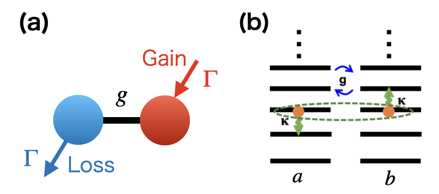
Figure A.1 : Illustration of (a) a typical $\mathcal{PT}$ symmetric system with a balanced gain and loss. Here, $\Gamma$ and g denote the strength of gain (loss) and interaction, and (b) the DDM in the Schiwnger boson representation.

	Non-Hermitian Hamiltonian	Lindbladian
Symmetry	$[H,PT]=0$	Strong Lindbladian $\mathcal{PT}$ symmetry $\eqref{HuberPT}$
Eigenvalues (fixed points)	Real$\to$ Complex conjugate pairs (i.e., a pair of stable and unstable eigenvalues)	Center (i.e., purely imaginary excitation spectrum) $\to$ Pairs of stable and unstable fixed points
Dynamics	Oscillation $\to$ Exponentially decay/divergence	Oscillation $\to$ Exponentially decay
Symmetry breaking	$\mathcal{PT}$ symmetry breaking of eigenvectors	$\mathcal{PT}$ symmetry breaking of solutions in the steady state
System size	Finite	Thermodynamic limit ($S\to\infty$)
Transition point	Exceptional point	CEP for the typical case

Table A.1 : Comparison between non-Hermitian $\mathcal{PT}$ transitions MostafazadehA1 ; Bender ; Bender2 and Lindbladian $\mathcal{PT}$ phase transitions Nakanishi1 ; Nakanishi2 .

Similarly, for the Lindbladian case with strong $\mathcal{PT}$ symmetry $\eqref{HuberPT}$, the phase transition occurs with spontaneous non-linear $\mathcal{PT}$ symmetry breaking, and the transition point is typically a CEP. Moreover, in the $\mathcal{PT}$ phase, persistent periodic oscillations appear, while in the $\mathcal{PT}$-broken phae, a pair of stable and unstable fixed points emerges.

Despite these similarities, we emphasize a fundamental difference: non-Hermitian $\mathcal{PT}$ transitions are generically spectral transitions occurring even in a finite system, while in the Lindbladian case, these are phase transitions in the steady state (including stationary oscillations) occurring only in the thermodynamic limit.

Lastly, we show that the one-collective spin model with strong Lindbladian $\mathcal{PT}$ symmetry $\eqref{HuberPT}$ can be regarded as a balanced gain and loss system in the Schwinger boson representation Pires . The Schwinger boson transformation is defined by

$$S_{x}=\frac{a^{\dagger}b+ab^{\dagger}}{2},\ \ S_{y}=\frac{a^{\dagger}b-ab^{\dagger}}{2i},\ \ S_{z}=\frac{a^{\dagger}a-b^{\dagger}b}{2},\ \ S=\frac{a^{\dagger}a+b^{\dagger}b}{2},$$ (A.3 )

where $a,b$ are bosonic annihilation operators. Here, the parity operation with $P=\exp(i\pi S_{x})$ on the internal degrees of freedom turns into an exchange of two subspaces, i.e., an operation on the external degrees of freedom, $PaP^{-1}=b$. In this case, the collective decay can be written as the product of gain (creation operator) and loss (annihilation operator) $S_{-}=ab^{\dagger}$. Therefore, one can intuitively understand that models with collective decay (excitation) exhibit a balanced gain and loss, and DCTCs (persistent oscillations) are caused by a sufficiently strong interaction canceling out gain and loss. As an example, we describe the illustration of the DDM ($H=gS_{x},\ L=\sqrt{\kappa/S}S_{-}$) in the Schwinger boson representation(Fig.A.1 (b)).

II B. Generalization of non-linear $\mathcal{PT}$ symmetry

In the main text, the nonlinear $\mathcal{PT}$ symmetry was defined as Eq.$\eqref{nonlinearPT}$, but here we will extend it for more general nonlinear dynamical systems. Let us consider a non-linear dynamical system described by non-linear Schr$\rm{\ddot{o}}$dinger equation $i\partial_{t}{\bf{q}}={\bf{f}}({\bf{q}})$, with a function ${\bf{f}}:\mathbb{C}^{n}\to\mathbb{C}^{n}$, and a vector ${\bf{q}}\in\mathbb{C}^{n}$ with $n\in\mathbb{N}$. Then, it is said to be $\mathcal{PT}$ symmetric if

$$P{\bf{f}}^{*}({\bf{q}}(t))={\bf{f}}({P\bf{q}^{*}}(-t)),$$ (B.1 )

where the asterisk denotes the complex conjugation. Then, if ${\bf{q}}(t)$ is a solution, then ${\bf{q}}^{*}(-t)$ is also one of the solutions.

We also say that the $\mathcal{PT}$ symmetry of the solution ${\bf{q}}(t)$ is unbroken if ${\bf{q}}(t)$ is equivalent to $PT{\bf{q}}(t)=P{\bf{q}}^{*}(-t)$ ,while if not, it is broken. Here, we say the two solutions are equivalent when they can be transformed from one to the other by using symmetry operations (other than the $\mathcal{PT}$ symmetry) that are present in the system. (For example, in a time-independent Lindbladian, the corresponding mean-field equation always has continuous time-translation symmetry. In this case, we say that ${\bf{q}}(t)$ is $\mathcal{PT}$-symmetric if ${\bf{q}}(t)=P{\bf{q}}^{*}(-t+t_{0})$, where $t_{0}\in\mathbb{R}$.)

III C. Theorems and proof about the relationship between the Lindbladian $\mathcal{PT}$ symmetry and the non-linear $\mathcal{PT}$ symmetry

Let us consider a dissipative one-collective spin model with strong Lindbladian $\mathcal{PT}$ symmetry (2) with $P=\exp(i\pi S_{x})$ described by the following GKSL equation,

$$\partial_{t}\rho=-iS[H,\rho]+S\sum_{\mu}\hat{\mathcal{D}}[L_{\mu}]\rho,$$ (C.1 )

where all the terms in the Hamiltonian and Lindblad operators are constructed by the normalized collective spin operators. In this case, the $\mathcal{PT}$-symmetric Hamiltonian can be written in general as,

$$H=\sum_{l,m,n}g_{lmn}(m_{x})^{l}(m_{y})^{m}(m_{z})^{2n},$$ (C.2 )

with $g_{lmn}\in\mathbb{R}$, and $l,m,n=\{0,1,2,...\}$. The Lindblad operator can be written in general as

$$L_{\mu}=\sum_{l,m,n}\gamma_{lmn}(m_{x})^{l}(m_{y})^{m}(m_{z})^{n},$$ (C.3 )

with $\gamma_{lmn}\in\mathbb{C}$ and its corresponding $\mathcal{PT}$ transformed Lindblad operator is give by

$$\tilde{L}_{\mu}:=PT(L_{\mu})^{\dagger}(PT)^{-1}=\sum_{l,m,n}\gamma_{lmn}(m_{x})^{l}(m_{y})^{m}(-m_{z})^{n}.$$ (C.4 )

We will prove Theorem 1 of the main text in subsection C.1 and Theorem 2, that is the extension to one-dimensional bosonic systems in subsection C.2.

III.1 C.1 Proof of Theorem 1

Theorem 1 For a dissipative one-collective spin model with the strong Lindbladian $\mathcal{PT}$ symmetry (2) where $P=\exp(i\pi S_{x})$, its mean-field non-linear dynamical system has $\mathcal{PT}$ symmetry $\eqref{nonlinearPT}$.

Proof.

First, let us consider the coherent (Hamiltonian) part. The time evolution of $x$-component of magnetization $m_{x}$ can be calculated as

$$\partial_{t}\braket{m_{x}} =iS\braket{[H,m_{x}]}$$

$$\approx\sum_{l,m,n}g_{lmn}(m\braket{m_{x}}^{l}\braket{m_{y}}^{m-1}\braket{m_{z}}^{2n-1}-2n\braket{m_{x}}^{l}\braket{m_{y}}^{m+1}\braket{m_{z}}^{2n+1})=:A_{H}(\braket{m_{x}},\braket{m_{y}},\braket{m_{z}}),$$ (C.5 )

where we use the mean-field approximation. One can easily find that $A_{H}(\braket{m_{x}},\braket{m_{y}},\braket{m_{z}})$ is the odd function with respect to $\braket{m_{z}}$. Similarly, the time evolution of $y,z$-component of magnetization $m_{y},\ m_{z}$ can be obtained as

$$\partial_{t}\braket{m_{y}} \approx\sum_{l,m,n}g_{lmn}(2n\braket{m_{x}}^{l+1}\braket{m_{y}}^{m}\braket{m_{z}}^{2n-1}-l\braket{m_{x}}^{l-1}\braket{m_{y}}^{m}\braket{m_{z}}^{2n+1})=:B_{H}(\braket{m_{x}},\braket{m_{y}},\braket{m_{z}}),$$

$$\partial_{t}\braket{m_{z}} \approx\sum_{l,m,n}g_{lmn}(l\braket{m_{x}}^{l-1}\braket{m_{y}}^{m+1}\braket{m_{z}}^{2n}-m\braket{m_{x}}^{l+1}\braket{m_{y}}^{m-1}\braket{m_{z}}^{2n})=:C_{H}(\braket{m_{x}},\braket{m_{y}},\braket{m_{z}}).$$ (C.6 )

This shows that the function $B_{H}(\braket{m_{x}},\braket{m_{y}},\braket{m_{z}})$ is odd and the function $C_{H}(\braket{m_{x}},\braket{m_{y}},\braket{m_{z}})$ is even with respect to $\braket{m_{z}}$.

Next, let us consider the dissipative part. A dissipative term of $x$-component of magnetization $m_{x}$ can be calculated as

$$S(2\braket{L_{\mu}^{\dagger}m_{x}L_{\mu}}-\braket{\{L_{\mu}^{\dagger}L_{\mu},m_{x}\}})\approx\sum_{v,v^{\prime}}\gamma^{*}\gamma^{\prime}\braket{m_{x}}^{l+l^{\prime}}\left[\braket{m_{y}}^{m+m^{\prime}-1}\braket{m_{z}}^{n+n^{\prime}+1}(-im+im^{\prime})+\braket{m_{y}}^{m+m^{\prime}+1}\braket{m_{z}}^{n+n^{\prime}-1}(in-in^{\prime})\right]$$

where $v=\{l,m,n\},\ \ v^{\prime}=\{l^{\prime},m^{\prime},n^{\prime}\}$ and $\gamma:=\gamma_{lmn}$, $\gamma^{\prime}:=\gamma_{l^{\prime}m^{\prime}n^{\prime}}$. Similarly, its corresponding dissipative term can be calculated as

$$S(2\braket{(\tilde{L}_{\mu})^{\dagger}m_{x}\tilde{L}_{\mu}}-\braket{\{(\tilde{L}_{\mu})^{\dagger}\tilde{L}_{\mu},m_{x}\}})$$

$$\approx\sum_{v,v^{\prime}}\gamma^{*}\gamma^{\prime}\braket{m_{x}}^{l+l^{\prime}}\left[\braket{m_{y}}^{m+m^{\prime}-1}(-\braket{m_{z}})^{n+n^{\prime}+1}(im-im^{\prime})+\braket{m_{y}}^{m+m^{\prime}+1}(-\braket{m_{z}})^{n+n^{\prime}-1}(-in+in^{\prime})\right].$$ (C.8 )

Adding $\eqref{P1L}$ to $\eqref{P2L}$, the time evolution of dissipative part of $x$-component can be written down as

$$\partial_{t}\braket{m_{x}}\approx A_{D}(\braket{m_{x}},\braket{m_{y}},\braket{m_{z}}):=$$

$$\sum_{v,v^{\prime}}\gamma^{*}\gamma^{\prime}\braket{m_{x}}^{l+l^{\prime}}\left[\braket{m_{y}}^{m+m^{\prime}-1}[\braket{m_{z}}^{n+n^{\prime}+1}-(-\braket{m_{z}})^{n+n^{\prime}+1}](-im+im^{\prime})+\braket{m_{y}}^{m+m^{\prime}+1}[\braket{m_{z}}^{n+n^{\prime}-1}-(-\braket{m_{z}})^{n+n^{\prime}-1}](in-in^{\prime})\right].$$ (C.9 )

Therefore, the function $A_{D}(\braket{m_{x}},\braket{m_{y}},\braket{m_{z}})$ is also odd with respect to $\braket{m_{z}}$. Similarly, one can show that the dissipative term of $y$-component is anti-symmetric with respect to $\braket{m_{z}}$ from the following calculation;

$$\partial_{t}\braket{m_{y}}\approx B_{D}(\braket{m_{x}},\braket{m_{y}},\braket{m_{z}}):=$$

$$\sum_{v,v^{\prime}}\gamma^{*}\gamma^{\prime}\braket{m_{y}}^{m+m^{\prime}}\left[\braket{m_{x}}^{l+l^{\prime}-1}[\braket{m_{z}}^{n+n^{\prime}+1}-(-\braket{m_{z}})^{n+n^{\prime}+1}](il-il^{\prime})+\braket{m_{x}}^{l+l^{\prime}+1}[\braket{m_{z}}^{n+n^{\prime}-1}-(-\braket{m_{z}})^{n+n^{\prime}-1}](-in+in^{\prime})\right].$$ (C.10 )

Moreover, the dissipative part of time evolution of $z$-component can be written down as

$$\partial_{t}\braket{m_{z}}\approx C_{D}(\braket{m_{x}},\braket{m_{y}},\braket{m_{z}}):=$$

$$\sum_{v,v^{\prime}}\gamma^{*}\gamma^{\prime}(\braket{m_{z}}^{n+n^{\prime}}+(-\braket{m_{z}})^{n+n^{\prime}})\left[\braket{m_{x}}^{l+l^{\prime}-1}\braket{m_{y}}^{m+m^{\prime}+1}(-il+il^{\prime})+\braket{m_{x}}^{l+l^{\prime}+1}\braket{m_{y}}^{m+m^{\prime}-1}(im-im^{\prime})\right].$$ (C.11 )

Then, one can easily find that the function $C_{D}(\braket{m_{x}},\braket{m_{y}},\braket{m_{z}})$ is also even with respect to $\braket{m_{z}}$. Thus, Eq.$\eqref{rarbthe}$ in the main text holds. Then, the non-linear dynamics of the magnetization ${\bf{m}}:=(\braket{m_{x}},\braket{m_{y}},\braket{m_{z}})$ satisfies the non-linear $\mathcal{PT}$ symmetry Eq.$\eqref{nonlinearPT}$ as

$$P{\bf{f}}^{*}({\bf{m}})=i\begin{pmatrix}-A(\braket{m_{x}},\braket{m_{y}},\braket{m_{z}})\\ -B(\braket{m_{x}},\braket{m_{y}},\braket{m_{z}})\\ C(\braket{m_{x}},\braket{m_{y}},\braket{m_{z}})\\ \end{pmatrix}=i\begin{pmatrix}A(\braket{m_{x}},\braket{m_{y}},-\braket{m_{z}})\\ B(\braket{m_{x}},\braket{m_{y}},-\braket{m_{z}})\\ C(\braket{m_{x}},\braket{m_{y}},-\braket{m_{z}})\\ \end{pmatrix}={\bf{f}}({P\bf{m}}),$$ (C.12 )

where $O(\braket{m_{x}},\braket{m_{y}},\braket{m_{z}}):=O_{H}(\braket{m_{x}},\braket{m_{y}},\braket{m_{z}})+O_{D}(\braket{m_{x}},\braket{m_{y}},\braket{m_{z}})$ ($O=A,B,C$) and the matrix $P$ is given by $P=\begin{pmatrix}1&&\\ &1&\\ &&-1\\ \end{pmatrix}$. ∎

III.2 C.2 Theorem 2 and its proof

Let us consider a dissipative one-dimmensional $j$-bosonic Hamiltonian described by the following GKSL equation,

$$\partial_{t}\rho=-iN[H,\rho]+N\sum_{\mu}\hat{\mathcal{D}}[L_{\mu}]\rho,$$ (C.13 )

where all the terms in the Hamiltonian and Lindblad operators are constructed by the normalized bosonic operators with system size parameter $N$. In this case, the Hamiltonian and Lindblad operators with strong Lindbladian $\mathcal{PT}$ symmetry (2) are given by

$$H=\sum_{\begin{subarray}{c}l_{i},m_{i}\\ i=1,...,j\end{subarray}}[g_{l_{1}m_{1}\cdots m_{j}}(a_{1}^{\dagger})^{l_{1}}(a_{1})^{m_{1}}\cdots(a_{j}^{\dagger})^{l_{j}}(a_{j})^{m_{j}}+g^{*}_{l_{1}m_{1}\cdots m_{j}}(a_{1}^{\dagger})^{l_{j}}(a_{1})^{m_{j}}\cdots(a_{j}^{\dagger})^{l_{1}}(a_{j})^{m_{1}}],$$ (C.14 )

with $g_{l_{1}m_{1}\cdots m_{j}}\in\mathbb{C}$ and

$$L_{\mu}=\sum_{\begin{subarray}{c}l_{i},m_{i}\\ i=1,...,j\end{subarray}}\gamma_{l_{1}m_{1}\cdots m_{j}}(a_{1}^{\dagger})^{l_{1}}(a_{1})^{m_{1}}\cdots(a_{j}^{\dagger})^{l_{j}}(a_{j})^{m_{j}},$$ (C.15 )

with $\gamma_{l_{1}m_{1}\cdots m_{j}}\in\mathbb{C}$ and its corresponding Lindblad operator is given by

$$\tilde{L}_{\mu}:=PTL^{\dagger}_{\mu}(PT)^{-1}=\sum_{\begin{subarray}{c}l_{i},m_{i}\\ i=1,...,j\end{subarray}}\gamma_{l_{1}m_{1}\cdots m_{j}}(a_{j}^{\dagger})^{m_{1}}(a_{j})^{l_{1}}\cdots(a_{1}^{\dagger})^{m_{j}}(a_{1})^{l_{j}},$$ (C.16 )

where bosonic operators are normalized by $\sqrt{N}$. Here, $l_{i},m_{i}=\{0,1,2,...\}$ for $\forall i$, and $Pa_{i}P^{-1}=a_{j-i+1}$. Note that the Hamiltonian is Hermitian $H=H^{\dagger}$ although not explicitly written in Eq.(C.14).

Theorem 2 For a one-dimensional bossnic systems with the strong Lindbladian $\mathcal{PT}$ symmetry (2) where the parity operator is the reflection of space, its mean-field non-linear dynamical system has $\mathcal{PT}$ symmetry.

Proof.

First, let us consider the coherent (Hamiltonian) part. The time evolution of order parameter $\braket{a_{i}}$ can be calculated as

$$i\partial_{t}\braket{a_{i}}\approx\sum_{\begin{subarray}{c}l_{i},m_{i}\\ i=1,...,j\end{subarray}}(g_{l_{1}m_{1}\cdots m_{j}}(\cdots\braket{a_{i}^{\dagger}}^{l_{i}-1}\cdots)+g^{*}_{l_{1}m_{1}\cdots m_{j}}(\cdots\braket{a_{i}^{\dagger}}^{l_{j-i+1}-1}\cdots)),$$ (C.17 )

where $(\cdots)$ denotes multiples of all the bosonic mean values other than $\braket{a_{i}}$. Similarly, the time evolution of order parameter $\braket{a_{j-i+1}}$ can be calculated as

$$i\partial_{t}\braket{a_{j-i+1}}\approx\sum_{\begin{subarray}{c}l_{i},m_{i}\\ i=1,...,j\end{subarray}}(g_{l_{1}m_{1}\cdots m_{j}}(\cdots\braket{a_{j-i+1}^{\dagger}}^{l_{j-i+1}-1}\cdots)+g^{*}_{l_{1}m_{1}\cdots m_{j}}(\cdots\braket{a_{j-i+1}^{\dagger}}^{l_{i}-1}\cdots)),$$ (C.18 )

where $(\cdots)$ denotes multiples of all the bosonic mean values other than $\braket{a_{j-i+1}}$. Then, the following relation can be deriven as

$$H^{*}_{a_{i}}(\braket{a_{j}}^{*},...,\braket{a_{1}}^{*})=H_{a_{j-i+1}}(\braket{a_{1}},...,\braket{a_{j}}),$$ (C.19 )

with $i\partial_{t}\braket{a_{i}}=H_{a_{i}}(\braket{a_{1}},...,\braket{a_{j}}).$

Next, let us consider the dissipative part. A term of the mean-field time evolution of the dissipative part can be calculated as

$$N(2\braket{L_{\mu}^{\dagger}a_{i}L_{\mu}}-\braket{\{L_{\mu}^{\dagger}L_{\mu},a_{i}\}})\approx\sum_{\begin{subarray}{c}l_{i},m_{i}\\ i=1,...,j\end{subarray}}\gamma^{*}\gamma^{\prime}(l_{i}^{\prime}\braket{a_{i}^{\dagger}}^{m_{i}+l_{i}^{\prime}-1}\braket{a_{i}}^{l_{i}+m_{i}^{\prime}}-m_{i}\braket{a_{i}^{\dagger}}^{l_{i}^{\prime}+m_{i}-1}\braket{a_{i}}^{l_{i}+m_{i}^{\prime}})(\cdots),$$ (C.20 )

where $\gamma:=\gamma_{l_{1}m_{1}\cdots m_{j}}$. The other term can be calculated as

$$N(2\braket{(\tilde{L}_{\mu})^{\dagger}a_{j-i+1}\tilde{L}_{\mu}}-\braket{\{(\tilde{L}_{\mu})^{\dagger}\tilde{L}_{\mu},a_{j-i+1}\}})\approx\sum_{\begin{subarray}{c}l_{i},m_{i}\\ i=1,...,j\end{subarray}}\gamma^{*}\gamma^{\prime}(m_{i}^{\prime}\braket{a_{j-i+1}^{\dagger}}^{l_{i}+m_{i}^{\prime}-1}\braket{a_{j-i+1}}^{m_{i}+l_{i}^{\prime}}-l_{i}\braket{a_{j-i+1}^{\dagger}}^{m_{i}^{\prime}+l_{i}-1}\braket{a_{j-i+1}}^{m_{i}+l_{i}^{\prime}})(\cdots).$$ (C.21 )

Then, it can be shown from Eqs.(C.20), (C.21),

$$G^{*}_{a_{i}}(\braket{a_{j}}^{*},...,\braket{a_{1}}^{*})=-G_{a_{j-i+1}}(\braket{a_{1}},...,\braket{a_{j}}),$$ (C.22 )

with $i\partial_{t}\braket{a_{i}}=iG_{a_{i}}(\braket{a_{1}},...,\braket{a_{j}}).$ Thus, similar to Theorem 1, the non-linear dynamical system has $\mathcal{PT}$ symmetry (B.1) with $P=P_{j}$ and ${\bf{q}}=(\braket{a_{1}},\braket{a_{2}},...,\braket{a_{j}})^{T}$, where $P_{j}$ is the $j\times j$ matrix given by

$$P_{j}=\left(\begin{array}[]{cccc}&&&1\\ &&1&\\ &\iddots&&\\ 1&&&\end{array}\right).$$ (C.27 )

∎

IV D. Analysis of Lindbladian $\mathcal{PT}$-symmetric one-collective spin models

IV.1 D.1 Continuous Lindbladian $\mathcal{PT}$ phase transition — Generalized DDM

In the generalized DDM with the Hamiltonian $H=2gS_{x}+\omega S_{z}^{2}/S$ and the Lindblad operator $L=\sqrt{\kappa/S}S_{-}$, there are distinct four fixed points; two $\mathcal{PT}$-symmetric ones ${\bf{m}}_{\pm,\rm{PT}}$ and two $\mathcal{PT}$-broken ones ${\bf{m}}_{\pm,\rm{PTb}}$. Former and latter solutions are given by

$${\bf{m}}_{\pm,\rm{PT}}=\left(\pm\sqrt{1-\left(\frac{\kappa}{g}\right)^{2}},\frac{\kappa}{g},0\right),$$ (D.1 )

and

$${\bf{m}}_{\pm,\rm{PTb}}=\left(\frac{g\omega}{\kappa^{2}+\omega^{2}},\frac{g\kappa}{\kappa^{2}+\omega^{2}},\pm\sqrt{1-\frac{g^{2}}{\kappa^{2}+\omega^{2}}}\right),$$ (D.2 )

respectively.

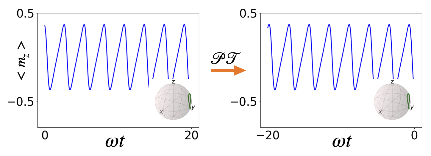
Figure D.1 : Dynamics of magnetization and the $\mathcal{PT}$ transform ($\braket{m_{z}}\to-\braket{m_{z}},\ t\to-t$) with $g=2$, $\omega=1$, and $\kappa=1.8$. inset: Their corresponding trajectory of magnetization’s dynamics. They describe the same attractors.

Let us perform the linear stability analysis for $m_{y}-m_{z}$ plane. Excitation spectra and modes at the $\mathcal{PT}$-symmetric solutions ${\bf{m}}_{\pm,\rm{PT}}$ $\eqref{fixedPT}$ are given by $\lambda=\{\sqrt{\alpha\beta},-\sqrt{\alpha\beta}\}$ and $\delta{\bf{m}}=\{(\sqrt{\alpha/\beta},1)^{T},\ (-\sqrt{\alpha/\beta},1)^{T}\}$ with

$$\sqrt{\alpha\beta} =2i(g^{2}-\kappa^{2})^{1/4}(\sqrt{g^{2}-\kappa^{2}}\mp\omega)^{1/2},$$ (D.3 )

$$\sqrt{\alpha/\beta} =i(g^{2}-\kappa^{2})^{1/4}(\sqrt{g^{2}-\kappa^{2}}\mp\omega)^{1/2}/g,$$ (D.4 )

where $\delta{\bf{m}}:=(\delta\braket{m_{y}},\delta\braket{m_{z}})$. The solution ${\bf{m}}_{+,\rm{PT}}$ is a center for $\kappa<\sqrt{g^{2}-\omega^{2}}$, and the solution ${\bf{m}}_{-,\rm{PT}}$ is also a center for $\kappa<g$. Indeed, $\mathcal{PT}$-symmetric persistent oscillations exist for $\kappa<g$ as shown in Fig.D.1. Moreover, the transition points $\kappa=g$ and $\kappa=\sqrt{g^{2}-\omega^{2}}$ are CEPs.

While, for the $\mathcal{PT}$-broken solutions ${\bf{m}}_{\pm,\rm{PTb}}$ $\eqref{fixedPT}$, excitation spectra and modes are given by

$$\lambda =\{2(\kappa+i\omega){m}_{\pm,\rm{PTb},z},\ 2(\kappa-i\omega){m}_{\pm,\rm{PTb},z}\},$$ (D.5 )

$$\delta{\bf{m}} =\{((\kappa+i\omega){m}_{\pm,\rm{PTb},z}/g,1)^{T},\ ((\kappa-i\omega){m}_{\pm,\rm{PTb},z}/g,1)^{T}\},$$ (D.6 )

where, ${m}_{\pm,\rm{PTb},z}$ is the $z$-component of ${\bf{m}}_{\pm,\rm{PTb}}$. Therefore, the solution ${\bf{m}}_{+,\rm{PTb}}$ is unstable for any $\kappa$, and the solution ${\bf{m}}_{-,\rm{PTb}}$ is stable for $\kappa>\sqrt{g^{2}-\omega^{2}}$. Moreover, a CEP appears at $\kappa=\sqrt{g^{2}-\omega^{2}}$ from the PPTB phase as well.

We note that the case for $\omega=0$ (i.e. DDM) is special such that effects of CEPs cannot be observed. Let us explain why this is so. To see effects of CEPs, one needs to choose an initial state in a different direction from its eigenmode $\delta{\bf{m}}=(0,1)$. However, to choose other directions $\delta{\bf{m}}=(a,b)$ with $a\neq 0,\ b\in\mathbb{C}$ is prohibited. This is because the magnetization’s vector $(m_{y},m_{z})=(1,0)$ is orthogonal to the eigenmode $\delta{\bf{m}}=(0,1)$ (left picture of Fig.D.2), and then it can not move in $m_{y}$ direction.

The other possibility to observe the effect of CEP is to choose the initial state in the $m_{x}$-direction. One can easily show that the Jacobian at $\mathcal{PT}$-symmetric solutions for $m_{x}-m_{z}$ plane is also given by the form of Eq.$\eqref{LL}$. However, for the DDM, the non-diagonalized elements simultaneously approach 0 at the transition point $\kappa=g$, indicating the absence of CEPs (right picture of Fig.D.2). Thus, effects of CEPs cannot be observed for the DDM.

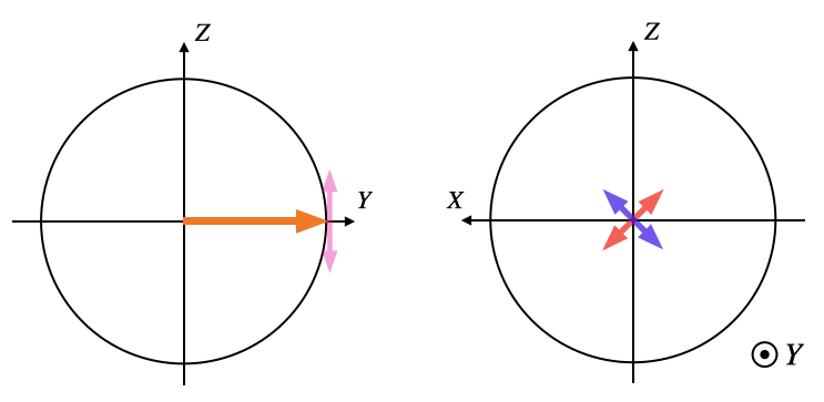
Figure D.2 : Left: The collective excitation mode (pink arrow) and the magnetization’s vector of the fixed point (orange arrow) at $\kappa=g$ for the DDM. Right: The collective excitation modes (blue and red or pink arrows). Here, the components of collective excitation modes are generally complex numbers, so we take absolute values for complex elements.

IV.2 D.2 Discontinuous Lindbladian $\mathcal{PT}$ phase transition — Dissipative LMG model.

Let us next consider a one-collective spin model with the Lipkin-Meshkov-Glick (LMG) Hamiltonian $H=g((S^{+})^{2}+(S^{-})^{2})/2S$ and the collective decay $L=\sqrt{\kappa/S}S_{-}$. In this model, a discontinuous phase transition occurs at $\kappa=g$ as shown in Fig.D.3 (a) Lee . One can easily find that this model has strong Linbdladian $\mathcal{PT}$ symmetry (2).

The time evolution of the dissipative LMG model is written down as

$$\partial_{t}{\bf{m}}=2\begin{pmatrix}-g\braket{m_{y}}\braket{m_{z}}+\kappa\braket{m_{x}}\braket{m_{z}}\\ -g\braket{m_{x}}\braket{m_{z}}+\kappa\braket{m_{y}}\braket{m_{z}}\\ 2g\braket{m_{x}}\braket{m_{y}}-\kappa(\braket{m_{x}}^{2}+\braket{m_{y}}^{2})\\ \end{pmatrix},$$ (D.7 )

where we have assumed that there is no quantum correlation in the initial state. The non-linear dynamical system (D.7) has $\mathcal{PT}$ symmetry (3).

There are distinct six fixed points; four $\mathcal{PT}$-symmetric ones and two $\mathcal{PT}$-broken ones. The $\mathcal{PT}$-symmetric solutions are given by

$${\bf{m}}_{\pm,\rm{PT}}^{\text{I}}=\left(M_{\pm},M_{\mp},0\right),\ \ \ {\bf{m}}_{\pm,\rm{PT}}^{\text{II}}=\left(-M_{\pm},-M_{\mp},0\right),$$ (D.8 )

with $M_{\pm}:=\sqrt{\frac{1\pm\sqrt{1-(\kappa/g)^{2}}}{2}}$. On the other hand, the $\mathcal{PT}$-broken solutions are given by

$${\bf{m}}_{\pm,\rm{PTb}}=\left(0,0,\pm 1\right).$$ (D.9 )

The elements in the Jacobian $\eqref{LL}$ at $\mathcal{PT}$-symmetric fixed points are given by

$$\alpha=-2gm_{x}+2\kappa m_{y},\ \ \beta=\frac{4}{m_{x}}(m_{x}^{2}-m_{y}^{2}),$$ (D.10 )

indicating that they are centers for $\kappa<g$, indicating the presence of persistent oscillations. This is consistent with Ref.Lee that reported that a periodic solution emerges, as shown in Fig.D.3 (b). Moreover, performing the $\mathcal{PT}$ transformation ($\braket{m_{z}}\to-\braket{m_{z}}$, $t\to-t$), one can find that they describe the same attractor. Therefore, this solution is $\mathcal{PT}$-symmetric. Moreover, this analysis shows that $\alpha=\beta=0$ at $\kappa=g$, so the period diverges at th transition point, but it is not a CEP.

Also, excitation spectra and modes around the $\mathcal{PT}$-broken fixed points ${\bf{m}}_{\pm,\rm{PTb}}$ are given by

$$\lambda =\{2(\kappa+g){{m}}_{\pm,\rm{PTb,z}},\ 2(\kappa-g){{m}}_{\pm,\rm{PTb,z}}\},$$ (D.11 )

$$\delta{\bf{m}} =\{(1,-1)^{T},\ (1,1)^{T}\},$$ (D.12 )

indicating that the solution ${\bf{m}}_{+,\rm{PTb}}$ is unstable for any $\kappa$ and the solution ${\bf{m}}_{-,\rm{PTb}}$ is stable for $\kappa<g$. Then, the solution ${\bf{m}}_{-,\rm{PTb}}$ is destabilized at $\kappa=g$ but a CEP does not appear from the $\mathcal{PT}$-broken phase as well. Fig.D.3 (c) shows the Lindbladian gap and the mean-field excitation spectrum. This result indicates that the mean-field prediction captures the discontinuous Lindbladian $\mathcal{PT}$ phase transition well for a large $S$.

Figure D.3 : The numerical analysis of the dissipative LMG model. (a) The normalized magnetization $\braket{m_{z}}$ in the stationary state $\lim_{t\to\infty}\rho(t)$ for some finite $S$ and mean field solution ($S=\infty$). (b) A time evolution of magnetization and the $\mathcal{PT}$ transform ($\braket{m_{z}}\to-\braket{m_{z}},\ t\to-t$) at $\kappa/g=0.8$. inset: Their corresponding trajectories. They describe the same attractor. (c) The Lindbladian gap $\Delta_{\text{gap}}$ for $S=30$ (blue dot) and the mean-field value $\Delta_{\text{mean}}$=2$(\kappa-g)$ (light blue line).

V E. Linear stability analysis around the $\mathcal{PT}$-broken fixed points

We consider the analysis around the $\mathcal{PT}$-broken fixed points with $\left.\braket{m_{z}}\right|_{ss}=Z,-Z\in\mathbb{R}$. From Eq.(4), the Jacobian can be written in the form

$$L=\left.\begin{pmatrix}\gamma_{1}\braket{m_{z}}&\alpha\\ \beta&\gamma_{2}\braket{m_{z}}\\ \end{pmatrix}\right|_{ss},$$ (E.1 )

where $\alpha,\ \beta,\gamma_{1}$, $\gamma_{2}\in\mathbb{R}$ depend on $\braket{m_{x}},\braket{m_{y}}$ and $\braket{m_{z}}^{2}$.

In this case, excitation spectrum and modes of Eq.(E.1) are given by

$$\lambda=\left.\frac{1}{2}\left((\gamma_{1}+\gamma_{2})\braket{m_{z}}\pm\sqrt{4\alpha\beta+(\gamma_{1}-\gamma_{2})^{2}\braket{m_{z}}^{2}}\right)\right|_{ss}$$ (E.2 )

and

$$\delta{\bf{m}}=\left(\left.-\frac{-(\gamma_{1}-\gamma_{2})\braket{m_{z}}\pm\sqrt{4\alpha\beta+(\gamma_{1}-\gamma_{2})^{2}\braket{m_{z}}^{2}}}{2\beta}\right|_{ss},1\right)^{T}.$$ (E.3 )

We assume that $\gamma_{1}+\gamma_{2}\neq 0$. For a pair of $\mathcal{PT}$-broken solutions $\left.\braket{m_{z}}\right|_{ss}=Z,-Z$ to be physical, the condition $\gamma_{1}\gamma_{2}\braket{m_{z}}^{2}>\alpha\beta$ is necessary. In this case, one is stable, but the other is unstable. Otherwise, there is always at least one eigenvalue with positive real part, and then both solutions are unstable. Moreover, a CEP typically emerges at the continuous phase transition point with $\left.\braket{m_{z}}\right|_{ss}=0$ and $\left.\alpha\beta\right|_{ss}=0$.

References

- (1) F. Wilczek, Quantum time crystals, Phys. Rev. Lett. 109, 160401 (2012).
- (2) K. Sacha and J. Zakrzewski, Time crystals: a review, Rep. Prog. Phys. 81 016401 (2018).
- (3) D. V. Else, C. Monroe, C. Nayak, and N. Y. Yao, Discrete time crystals, Annu. Rev. Condens. Matter Phys. 11, 467 (2020).
- (4) H. Watanabe and M. Oshikawa, Absence of quantum time crystals, Phys. Rev. Lett. 114, 251603 (2015).
- (5) F. Iemini, A. Russomanno, J. Keeling, M. Schir, M. Dalmonte, and R. Fazio, Boundary time crystals, Phys. Rev. Lett. 121, 35301 (2018).
- (6) F. Minganti, I. I. Arkhipov, A. Miranowicz, and F. Nori, Correspondence between dissipative phase transitions of light and time crystals, arXiv:2008.08075.
- (7) C. Booker, B. Buča, and D. Jaksch, Non-stationarity and dissipative time crystals: spectral properties and finite-size effects, New J. Phys. 22 085007 (2020).
- (8) C. Lled and M. H. Szymaska, A Dissipative time crystal with or without Z2 symmetry breaking, New J. Phys. 22 075002 (2020).
- (9) G. Piccitto, M. Wauters, F. Nori, and N. Shammah, Symmetries and conserved quantities of boundary time crystals in generalized spin models, Phys. Rev. B 104, 014307 (2021).
- (10) L. F. dos Prazeres, L. da S. Souza, and F. Iemini, Boundary time crystals in collective -level systems, Phys. Rev. B 103, 184308 (2021).
- (11) G. Passarelli, P. Lucignano, R. Fazio, and A. Russomanno, Dissipative time crystals with long-range Lindbladians, Phys. Rev. B 106, 224308 (2022).
- (12) Ya-Xin Xiang, Qun-Li Lei, Zhengyang Bai, Yu-Qiang Ma, Self-organized time crystal in driven-dissipative quantum system, arXiv preprint arXiv:2311.08899.
- (13) S. Yang, Z. Wang, L. Fu, and J. Jie, Emergent continuous time crystal in dissipative quantum spin system without driving, arXiv:2403.08476v1.
- (14) P. Kongkhambut, J. Skulte, L. Mathey, J. G. Cosme, A. Hemmerich, and H. Keßler, Observation of a continuous time crystal, Science 377, 670 (2022).
- (15) X. Wu, Z. Wang, F. Yang, R. Gao, C. Liang, M. K. Tey, X. Li, T. Pohl, L. You, Observation of a dissipative time crystal in a strongly interacting Rydberg gas, arXiv:2305.20070.
- (16) Y. Jiao, W. Jiang, Y. Zhang, J. Bai, Y. He, H. Shen, J. Zhao, S. Jia, Observation of a time crystal comb in a driven-dissipative system with Rydberg gas, arXiv:2402.13112.
- (17) YH. Chen and X. Zhang, Realization of an inherent time crystal in a dissipative many-body system. Nat Commun 14, 6161 (2023).
- (18) A. Greilich, N.E. Kopteva, A.N. Kamenskii, P.S. Sokolov, V.L. Korenev and M. Bayer, Robust continuous time crystal in an electron–nuclear spin system. Nat. Phys. 20, 631–636 (2024).
- (19) Y. Nakanishi, T. Sasamoto, Dissipative time crystals originating from parity-time symmetry, Phys. Rev. A 107, L010201(2023).
- (20) B. Buča and T. Prosen, A note on symmetry reductions of the Lindblad equation: transport in constrained open spin chains, New J. Phys. 14 073007 (2012).
- (21) A Lindbladian is said to have strong unitary symmetry when with any operator Buca2 . Then, the mean value of is conserved, .
- (22) J. Huber, P. Kirton, S. Rotter, P. Rabl, Emergence of -symmetry breaking in open quantum systems, SciPost Phys. 9, 52 (2020).
- (23) V. V. Konotop, J. Yang, and D. A. Zezyulin, Nonlinear waves in -symmetric systems, Rev. Mod. Phys. 88, 035002 (2016).
- (24) M. Fruchart, R. Hanai, P. B. Littlewood, and V. Vitelli, Non-reciprocal phase transitions, Nature 592, 363-369 (2021).
- (25) Z. You, A. Baskaran, and M. C. Marchetti, Nonreciprocity as a Generic Route to Traveling States, Proc. Natl. Acad. Sci. U.S.A. 117, 19767 (2020).
- (26) S. Saha, J. Agudo-Canalejo, and R. Golestanian, Scalar Active Mixtures: The Nonreciprocal Cahn-Hilliard Model, Phys. Rev. X 10, 041009 (2020).
- (27) R. Hanai, A. Edelman, Y. Ohashi, and P. B. Littlewood, Non-Hermitian phase transition from a polariton Bose-Einstein condensate to a photon laser, Phys. Rev. Lett. 122, 185301(2019).
- (28) R. Hanai and P. B. Littlewood, Critical fluctuations at a many-body exceptional point, Phys. Rev. Res. 2, 033018(2020).
- (29) T. Suchanek, K. Kroy, and S. A. M. Loos, Entropy production in the nonreciprocal Cahn-Hilliard model, Phys. Rev. E 108, 064610 (2023).
- (30) C. P. Zelle, R. Daviet, A. Rosch, and S. Diehl, Universal phenomenology at critical exceptional points of nonequilibrium models, arXiv:2304.09207 (2023).
- (31) E. I. R. Chiacchio, A. Nunnenkamp, and M. Brunelli, Nonreciprocal Dicke Model, Phys. Rev. Lett. 131, 113602 (2023).
- (32) T. Nadolny, C. Bruder, M. Brunelli, Nonreciprocal synchronization of active quantum spins, arXiv:2406.03357.
- (33) As we have shown in the main text, DCTCs in open quantum systems can be understood as a symmetric phase of the dynamical systems described by the nonlinear Schrödinger-type equation, , where the -symmetry is defined as . Non-reciprocal phase transitions Fruchart ; You ; Saha , on the other hand, corresponds to a spontaneous symmetry breaking of anti--symmetry, . [Note that in Ref. Fruchart , they called their transition -symmetry breaking instead of anti--symmetry breaking, which is merely the difference in the convention.] This difference arises due to the property that the order-parameter dynamics of our open quantum systems are described by the form similar to nonlinear Schrödinger equation, , while those considered in active matter systems are overdamped, , where the factor “” in front of the time-derivative on the left-hand side is missing compared to the open quantum system analog.
- (34) J. Hannukainen and J. Larson, Dissipation-driven quantum phase transitions and symmetry breaking, Phys. Rev. A 98, 042113 (2018).
- (35) D. A. Lidar, I. L. Chuang, and K. B. Whaley, Decoherence-Free Subspaces for Quantum Computation, Phys. Rev. Lett. 81, 2594 (1998).
- (36) B. Buča, J. Tindall, and D. Jaksch, Non-stationary coherent quantum many-body dynamics through dissipation, Nat. Commun. 10, 1730 (2019).
- (37) G. Lindblad, On the generators of quantum dynamical semigroups, Commun. Math. Phys. 48, 119 (1976).
- (38) V. Gorini, A. Kossakowski, E. C. G. Sudarshan, Completely positive dynamical semi-groups of -level systems, J. Math. Phys. 17, 821 (1976).
- (39) Á. Rivas and S. F. Huelga, Open Quantum Systems: An Introduction, SpringerBriefs in Physics (Springer, Heidelberg, 2012).
- (40) H. P. Breuer and F. Petruccione, The Theory of Open Quantum Systems, (Oxford University Press, Oxford, 2002).
- (41) E. M. Kessler, G. Giedke, A. Imamoglu, S. F. Yelin, M. D. Lukin, and J. I. Cirac, Dissipative phase transition in a central spin system, Phys. Rev. A 86, 012116 (2012).
- (42) F. Minganti, A. Biella, N. Bartolo, C. Ciuti, Spectral theory of Liouvillians for dissipative phase transitions, Phys. Rev. A 98, 042118 (2018).
- (43) J. Huber, P. Kirton, P. Rabl, Nonequilibrium magnetic phases in spin lattices with gain and loss, Phys. Rev. A 102, 012219 (2020).
- (44) Y. Nakanishi, T. Sasamoto, phase transition in open quantum systems with Lindblad dynamics, Phys. Rev. A 105, 022219 (2022).
- (45) C. M. Bender, S. Boettcher, Real spectra in non-hermitian hamiltonians having symmetry, Phys. Rev. Lett. 80, 5243 (1998); PT-symmetric quantum mechanics, J. Math. Phys. 40, 2201 (1999).
- (46) C. M. Bender, Introduction to PT-symmetric quantum theory, Contemp. Phys. 46, 277 (2005); Making sense of nonHermitian Hamiltonians, Rep. Prog. Phys. 70, 947 (2007).
- (47) A. Mostafazadeh, Pseudo-Hermiticity versus PT symmetry: The necessary condition for the reality of the spectrum of a non-Hermitian Hamiltonian, J. Math. Phys. 43, 205 (2002).
- (48) T. Prosen, -symmetric quantum Liouvillian dynamics, Phys. Rev. Lett. 109, 090404 (2012).
- (49) T. Prosen, Generic examples of -symmetric qubit (spin-1/2) Liouvillian dynamics, Phys. Rev. A 86, 044103 (2012).
- (50) D. Huybrechts, F. Minganti, F. Nori, M. Wouters, N. Shammah, Validity of mean-field theory in a dissipative critical system: Liouvillian gap, -symmetric antigap, and permutational symmetry in the XYZ model, Phys. Rev. B 101, 214302 (2020).
- (51) L. Sá, P. Ribeiro, and T. Prosen, Symmetry classification of many-body Lindbladians: Tenfold way and beyond, Phys. Rev. X 13, 031019 (2023).
- (52) The weak Lindbladian symmetry is defined as with Prosen3 . Here, () is a parity (time-reversal) superoperator, and .
- (53) L. S. Souza, L. F. dos Prazeres, and F. Iemini, Sufficient condition for gapless spin-boson Lindbladians, and its connection to dissipative time crystals, Phys. Rev. Lett. 130, 180401 (2023).
- (54) See the Supplemental material for the details.
- (55) S. Strogatz, Nonlinear Dynamics and Chaos: With Applications to Physics, Biology, Chemistry, and Engineering (CRC Press, Boca Raton, FL, 2018).
- (56) The emergence of DCTCs can be intuitively understood in the Schwinger boson representation. In this representation, the model exhibits a balanced gain and loss, and DCTCs are caused by a sufficiently strong interaction that cancels out gain and loss. (See Supplemental Materials A).
- (57) The DDM (i.e., ) is a subtle case where a CEP appears but its effects cannot be observed. This is because the fluctuation vector orthogonal to the zero excitation mode coincides with the normal vector but this cannot be excited because has to be conserved (see Supplemental Material D).
- (58) A. S. T. Pires, Theoretical tools for spin models in magnetic systems (IOP, Bristol, UK, 2021).
- (59) T. E. Lee, C. Chan, and S. F. Yelin, Dissipative phase transitions: Independent versus collective decay and spin squeezing, Phys. Rev. A 90, 052109 (2014).