A geometric approach to informed MCMC sampling

Abstract

A Riemannian geometric framework for Markov chain Monte Carlo (MCMC) is developed where using the Fisher-Rao metric on the manifold of probability density functions (pdfs) informed proposal densities for Metropolis-Hastings (MH) algorithms are constructed. We exploit the square-root representation of pdfs under which the Fisher-Rao metric boils down to the standard $L^{2}$ metric on the positive orthant of the unit hypersphere. The square-root representation allows us to easily compute the geodesic distance between densities, resulting in a straightforward implementation of the proposed geometric MCMC methodology. Unlike the random walk MH that blindly proposes a candidate state using no information about the target, the geometric MH algorithms effectively move an uninformed base density (e.g., a random walk proposal density) towards different global/local approximations of the target density. We compare the proposed geometric MH algorithm with other MCMC algorithms for various Markov chain orderings, namely the covariance, efficiency, Peskun, and spectral gap orderings. The superior performance of the geometric algorithms over other MH algorithms like the random walk Metropolis, independent MH and variants of Metropolis adjusted Langevin algorithms is demonstrated in the context of various multimodal, nonlinear and high dimensional examples. In particular, we use extensive simulation and real data applications to compare these algorithms for analyzing mixture models, logistic regression models and ultra-high dimensional Bayesian variable selection models. A publicly available R package accompanies the article.

Keywords:  Bayesian models, Markov chain Monte Carlo, Metropolis-Hastings, Riemann manifolds, variable selection

1 Introduction

Sampling from complex, high dimensional, discreet, and continuous probability distributions is a common task arising in diverse scientific areas, such as machine learning, physics, and statistics. Markov chain Monte Carlo (MCMC) is the most popular method for sampling from such distributions and among the different MCMC algorithms, Metropolis-Hastings (MH) algorithms (Metropolis et al., 1953; Hastings, 1970) are predominant. In MH algorithms, given the current state $x$, a proposal $y$ is drawn from a density $f(y|x)$, which is then accepted with a certain probability. The random walk MH (RWM) algorithms use a symmetric $f$, that is $f(y|x)=f(x|y)$, for example when $y=x+I$ with the increment $I$ following a normal/uniform density centered at the origin (Robert and Casella, 2004, chap. 7.5). The RWM algorithms are easy to implement, but since the proposal density $f$ does not use any information on the target density $\psi$, RWM can suffer from slow convergence, particularly in high dimensions (Neal, 2003). This led to the development of alternative MH proposals that exploit some information about the target density $\psi$. Intuitively, the informed MCMC schemes can avoid frequent visits to states with low target probabilities leading to faster convergence. Indeed, for sampling from continuous target densities, informative MH proposals such as those of the Metropolis adjusted Langevin algorithms (MALA) (Rossky et al., 1978; Besag, 1994; Roberts and Tweedie, 1996) and Hamiltonian Monte Carlo (HMC) algorithms (Duane et al., 1987) have been constructed employing the gradient of the log of the target density.

However, the standard MALA and HMC algorithms do not efficiently sample from high dimensional distributions with complex structures such as strong dependencies between variables, non-Gaussian shapes, or multiple modes (Girolami and Calderhead, 2011; Betancourt, 2013; Roy and Zhang, 2023). Also, as mentioned in Girolami and Calderhead (2011), ‘the tuning of these MCMC methods remains a major issue’. The Euclidean MALA and HMC algorithms fail to take into account the geometry of the target distribution in the selection of step sizes. Indeed, using ideas from information geometry, Girolami and Calderhead (2011) constructed manifold MALA and HMC methods called the manifold MALA (MMALA) and the Riemannian manifold HMC (RMHMC), respectively. MMALA and RMHMC adapt to the second-order geometric structure of the target, which allows these algorithms to align their proposals in the direction of the target that exhibits the greatest local variation and generally outperform their Euclidean counterparts in exploring high dimensional complex target distributions (Brofos et al., 2023; Girolami and Calderhead, 2011). However, the sophisticated form of the Hamiltonian employed in RMHMC necessitates the use of complex numerical integrators that are significantly more expensive than the numerical integrator employed in HMC. Since these manifold variants of MALA and HMC use a position-specific metric, it needs to be recomputed in every iteration, and generally, this computation scales cubically. Also, for implementing these manifold chains, first and higher-order derivatives of the log target density are required. One must find appropriate alternatives if these derivatives are not available in closed form. Also, MALA and HMC algorithms are not applicable for discrete distributions, although there have been some recent developments to extend these methods to form informative MH proposals for discrete spaces by emulating the behavior of gradient-based MCMC samplers on Euclidean spaces (see e.g. Zanella, 2020; Zhang et al., 2022; Nishimura et al., 2020; Pakman and Paninski, 2013). On the other hand, as mentioned in Zanella (2020), it is ‘typically not feasible’ to sample from their informed proposals in continuous state spaces.

In this article, we propose an original Riemannian geometric framework for developing informative MH proposals, irrespective of whether the state space is discrete or continuous. In RWM, the current state $x$ is blindly moved to $x+I$ following a Euclidean random perturbation $I$, failing to take into account the non-Euclidean nature of the target space. On the other hand, starting with a ‘base’, uninformed kernel $f$, our proposed method moves $f$ in the directions of $\psi$ to produce informed MH proposals. Our novel formulation has the merit of being straightforward and universally applicable to both discrete and continuous spaces exploiting their natural Riemannian geometry. The Fisher-Rao (FR) metric that we consider here is the ‘natural’ metric on the space of probability density functions (pdfs) (Rao, 1945) and it is known that the gradient under the FR metric is the fastest ascending direction of a distribution objective function (Amari, 1998). Thus, the FR metric should ideally be used to explore a distribution, although, as noted before, for manifold variants of MALA and HMC, the use of this metric generally leads to higher computational burden.

To build computationally efficient, informative MCMC algorithms that adapt to the geometry of the target, we consider a novel approach using Bhattacharyya’s (1943) ‘square-root’ representation for pdfs. Under this representation, the manifold of pdfs can be identified with the positive orthant of the unit sphere and the FR metric boils down to the standard $L^{2}$ metric (see Figure 1). This simplifies computations through the availability of explicit, closed-form expressions for useful geometric quantities like geodesic paths, distances as well as exponential and inverse-exponential maps. Thus, the proposed general-purpose, geometric MCMC algorithms, unlike MMALA and RMHMC, do not require the first and higher-order derivatives of the log target density. Also, Zanella (2020) considers point-wise informed proposals for discrete spaces, whereas here, we construct informed proposals respecting the geometry of the space of pdfs applicable to both discrete and continuous spaces.

We provide new results based on Peskun, covariance, efficiency and spectral gap orderings for comparing Markov chains with the same stationary distribution. These general theoretical results are then used to demonstrate the improvement obtained by the proposed geometric method over the uninformed base Markov chains. It is known that the spectral gap is closely related to the convergence properties of a Markov chain. Thus, the geometric MCMC leads to superior convergence properties over the base RWM, independent MH, or other Markov chain kernels. For RWM algorithms to be geometrically ergodic, it is necessary that the invariant density $\psi$ has moment generating function (Jarner and Tweedie, 2003), although for heavy-tailed target distributions, the RWM chains can have a polynomial rate of convergence (Jarner and Roberts, 2007). Mengersen and Tweedie (1996) proved that when the support of $\psi$ is $\mathbb{R}$, the RWM chain cannot be uniformly ergodic. The geometric, polynomial, and uniform ergodicity definitions can be found in Douc et al. (2018). We provide examples where the proposed geometric MH chain is uniformly ergodic, whereas the MH chains with the base RWM or independent kernels are not even geometrically ergodic. Johnson and Geyer (2012) considered RWM for densities induced by appropriate transformations to obtain geometric ergodicity for RWM algorithms even when the original target density is sub-exponential. This variable transformation method works for densities with continuous variables, and as mentioned in Johnson and Geyer (2012), it may cause other problems. For example, the induced density can be multimodal even if the original density is not. This article’s extensive examples involving discrete and continuous spaces using simulated and real data show orders of magnitude improvements in geometric MCMC compared to RWM, independent MH, and other MCMC algorithms.

The rest of the article is organized as follows. Section 2 introduces the square-root representation and the FR Riemannian geometric framework. In Section 3, we define the informed proposal distributions constructed by ‘moving’ any base uninformed kernel in the directions of the target density and its local and global approximations. Section 4 provides some results for comparing general state space Markov chains. Then, Section 5 uses these general results to establish the superior performance of the proposed geometric MCMC algorithms over the MH algorithms based on the uninformed base kernel. Section 6 describes some methods for sampling from the geometric proposal distributions for efficient simulation using the proposed MH algorithms. In Section 7, we consider several widely used high dimensional and nonlinear models with complex, multimodal target distributions, namely mixture models, logistic models, and the Bayesian variable selection models with spike and slab priors. While the target distribution for the feature selection example is discrete, it is continuous for the other examples. The proposed geometric methods outperform several traditional and state-of-the-art MCMC algorithms in all these examples. Finally, in Section 8 we discuss possible extensions and future works. The appendix contains an alternative formulation of the geometric MCMC method and results from additional simulation studies for the Bayesian variable selection example. The paper is accompanied by an R package geommc.

2 Square-root representation and Fisher-Rao metric

Let $\mathcal{F}=\{f\mathrel{\mathop{\mathchar 58\relax}}f\mathrel{\mathop{\mathchar 58\relax}}\mathbb{R}\rightarrow\mathbb{R}_{+}\cup\{0\}\;\mbox{with}\;\int_{\mathbb{R}}f(x)dx=1\}$ be the space of all pdfs on $\mathbb{R}$. To keep the notations simpler, in this section, we make the presentation in the context of densities on $\mathbb{R}$ although it straightforwardly extends to higher dimensions. For $f\in\mathcal{F}$, $T_{f}\mathcal{F}=\{\partial f\mathrel{\mathop{\mathchar 58\relax}}\mathbb{R}\rightarrow\mathbb{R}\;\mbox{with}\;\int_{\mathbb{R}}\partial f(x)f(x)dx=0\}$ is the tangent space, which is a linear space. Thus, $T_{f}\mathcal{F}$ can be viewed as the set of all possible perturbations of $f$. The Fisher-Rao (FR) metric (Rao, 1945) is defined as

$$\langle\partial f_{1},\partial f_{2}\rangle_{f}=\int_{\mathbb{R}}\partial f_{1}(x)\partial f_{2}(x)\frac{1}{f(x)}dx.$$

Although the FR metric has several advantages, computing geodesic paths and distances for it are difficult. One solution is to consider Bhattacharyya’s (1943) ‘square-root’ representation $\xi\mathrel{\mathop{\mathchar 58\relax}}\mathcal{F}\rightarrow\mathcal{M}$ given by $\xi(f)=\sqrt{f}$, where $\mathcal{M}=\{\rho\mathrel{\mathop{\mathchar 58\relax}}\mathbb{R}\rightarrow\mathbb{R}_{+}\cup\{0\}\;\mbox{with}\;\int_{\mathbb{R}}\rho^{2}(x)dx=1\}$ (see Figure 1). We will use the inverse map $\xi^{-1}(\rho)=\rho^{2}=f$ to take $\rho$ back to $\mathcal{F}$, the space of densities. The square-root representation has previously been used in shape analysis (Srivastava et al., 2010), variational Bayes (Saha et al., 2019), sensitivity analysis (Kurtek and Bharath, 2015), quantum estimation theory (Facchi et al., 2016) among other areas.

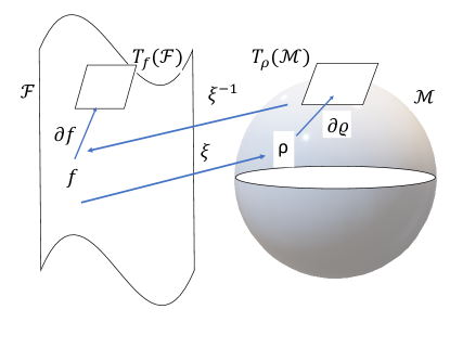
Figure 1: The square root transformation from $\mathcal{F}$, the space of pdfs to $\mathcal{M}$, the positive orthant of the unit sphere.

Note that $\mathcal{M}$ is the positive orthant of the unit sphere, where the FR metric boils down to the standard $L^{2}$ metric $\langle\rho_{1},\rho_{2}\rangle=\int_{\mathbb{R}}\rho_{1}(x)\rho_{2}(x)dx$ and geodesic paths and distances are available in closed form. Indeed, the geodesic distance between $\rho_{1}$ and $\rho_{2}$ in $\mathcal{M}$ is the angle between them $\theta=\cos^{-1}\langle\rho_{1},\rho_{2}\rangle$. Note that, for identical distributions $\rho_{1}=\rho_{2}$ implying $\theta=0$. Also, by Jensen’s inequality, $\langle\rho_{1},\rho_{2}\rangle=\langle f_{1},\rho_{2}/\rho_{1}\rangle\leq 1$ implying that $\theta$ is bounded above by the right angle providing an upper bound to the geodesic distance between pdfs. Also, the geodesic path between $\rho_{1}$ and $\rho_{2}$ indexed by $r\in[0,1]$ is $\varsigma(r)=[\sin(\theta)]^{-1}[\rho_{1}\sin(\theta-r\theta)+\rho_{2}\sin(r\theta)]$.

Note that, for $\rho\in\mathcal{M}$, the tangent space $T_{\rho}\mathcal{M}=\{\partial\rho\mathrel{\mathop{\mathchar 58\relax}}\langle\partial\rho,\rho\rangle=0\}$ is a linear space. In analogy to vector addition $x+v$ in linear space that moves a point $x$ along the straight line in the direction of $v$, we define the exponential map $\exp_{\rho_{1}}\mathrel{\mathop{\mathchar 58\relax}}T_{\rho_{1}}\mathcal{M}\rightarrow\mathcal{M}$ as moving a point $\rho_{1}$ along the geodesic tangent to $\partial\rho$ at $\rho_{1}$ and is defined as $\exp_{\rho_{1}}(\partial\rho)=\cos(\|\partial\rho\|)\rho_{1}+\sin(\|\partial\rho\|)\partial\rho(\|\partial\rho\|)^{-1}$ where $\|\cdot\|$ is the $L_{2}$ norm. The inverse exponential map $\exp^{-1}_{\rho_{1}}\mathrel{\mathop{\mathchar 58\relax}}\mathcal{M}\rightarrow T_{\rho_{1}}\mathcal{M}$ is given by $\exp^{-1}_{\rho_{1}}(\rho_{2})=\theta[\sin(\theta)]^{-1}(\rho_{2}-\cos(\theta)\rho_{1})$ and it is used to map points from the representation space to the tangent space.

Unlike a linear space for which the tangent space is the same everywhere, it is not true for a general manifold. Fortunately, the parallel transport $\Gamma_{\rho_{1}}^{\rho_{2}}\mathrel{\mathop{\mathchar 58\relax}}T_{\rho_{1}}\mathcal{M}\rightarrow T_{\rho_{2}}\mathcal{M}$ provides a link between tangent spaces at different points along geodesic paths (great circles) in $\mathcal{M}$. For $\partial\rho\in T_{\rho_{1}}\mathcal{M},\Gamma_{\rho_{1}}^{\rho_{2}}(\partial\rho)=\partial\rho-2\langle\partial\rho,\rho_{2}\rangle(\rho_{1}+\rho_{2})/\|\rho_{1}+\rho_{2}\|$.

3 Manifold MH proposals

Let $\psi$ be the target density on X with respect to some measure $\mu$. MCMC algorithms simulate a Markov chain $\{X^{(n)}\}_{n\geq 1}$ with some Markov transition function (Mtf) $Q(x,dy)$ that has $\psi$ as its stationary density. While appropriate choices of $Q$ that uses information on $\psi$ results in a fast mixing Markov chain, bad, uninformed choices can take weeks or even months to converge to $\psi$. To develop informative MCMC schemes that adapt to the geometry of the target distribution, starting with any ‘baseline’ proposal density $f(y|x)$, we construct geometric MH proposals by perturbing $f$ in the directions of $\psi$ or some approximations of $\psi$.

Let $\mathcal{G}=\{g_{1},g_{2},\dots,g_{k}\}$ be a set of $k$ pdfs representing different (local/global) approximations of the target density. Later in this section, we discuss possible choices for $\mathcal{G}$. For a given ‘baseline’ density $f$, the inverse exponential map $\chi_{g_{i}}\equiv\exp^{-1}_{\sqrt{f}}(\sqrt{g_{i}})$ takes the density to the tangent space $T_{\sqrt{f}}\mathcal{M}$, and then for a given step size $\epsilon$, the exponential map $\exp_{\sqrt{f}}(\epsilon\exp^{-1}_{\sqrt{f}}(\sqrt{g_{i}}))=\exp_{\sqrt{f}}(\epsilon\chi_{g_{i}})$ takes it back to $\mathcal{M}$ (Figure 2). Using the transformation $\xi^{-1}$ defined in Section 2, we construct a ‘perturbed’ pdf $\{\exp_{\sqrt{f}}(\epsilon\chi_{g_{i}})\}^{2}$. For this perturbed density by varying $\epsilon$ from zero and one, the geodesic path from $f$ to $g_{i}$ can be traced. Note that, $\{[\exp_{\sqrt{f}}(\epsilon\chi_{g_{i}})]^{2},i=1,\dots,k\}$ is the set of $\epsilon$-perturbations of $f$ along the directions specified by $\mathcal{G}$. We use these geometrically perturbed densities to form informative proposals for MH algorithms. Indeed, the proposed geometric proposals use these densities to move an uninformed baseline density $f$ along different approximations of the target density $\psi$.

Recall that, in an RWM chain, given the current state $x$, an increment (step size) $I$ is proposed according to a fixed density to move to the candidate point $y=x+I$. Thus, the random perturbation $I$ used for local exploration in the RWM algorithm does not take into account the non-Euclidean structure of the target parameter space. On the other hand, the step size and the directions used in the geometric proposal density respect the geometry of pdfs.

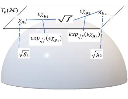
Figure 2: Geometric $\epsilon$ perturbation of $\sqrt{f}$ in the direction of $\sqrt{g_{i}},i=1,2$.

Proposition 1.

Given densities $f$ and $g_{i}$, $\{\exp_{\sqrt{f}}(\epsilon\exp^{-1}_{\sqrt{f}}(\sqrt{g_{i}}))\}^{2}(y|x)$ is a pdf for $\epsilon\in[0,1]$, with

$$\big{\{}\exp_{\sqrt{f}}(\epsilon\exp^{-1}_{\sqrt{f}}(\sqrt{g_{i}}))\big{\}}^{2}(y|x)$$

$$=\cos^{2}(\epsilon\theta_{i,x})f(y|x)+\sin^{2}(\epsilon\theta_{i,x})h_{i}(y|x)+\sin(2\epsilon\theta_{i,x})\sqrt{f(y|x)}\zeta_{i}(y|x),$$ (1)

where $\theta_{i,x}=\cos^{-1}\big{\langle}\sqrt{f(y|x)},\sqrt{g_{i}(y|x)}\big{\rangle}$,

$$\zeta_{i}(y|x)=\frac{\sqrt{g_{i}(y|x)}-\sqrt{f(y|x)}\big{\langle}\sqrt{f(y|x)},\sqrt{g_{i}(y|x)}\big{\rangle}}{\sqrt{1-\big{\langle}\sqrt{f(y|x)},\sqrt{g_{i}(y|x)}\big{\rangle}^{2}}},$$ (2)

and $h_{i}(y|x)=\zeta^{2}_{i}(y|x)$.

Proof.

We have

$$\exp_{\sqrt{f}}(\epsilon\exp^{-1}_{\sqrt{f}}(\sqrt{g_{i}}))(y|x)=\cos\big{(}\epsilon\theta_{i,x}[\sin(\theta_{i,x})]^{-1}\big{\|}\sqrt{g_{i}(y|x)}-\sqrt{f(y|x)}\cos(\theta_{i,x})\big{\|}\big{)}$$

$$\sqrt{f(y|x)}+\sin\big{(}\epsilon\theta_{i,x}[\sin(\theta_{i,x})]^{-1}\big{\|}\sqrt{g_{i}(y|x)}-\sqrt{f(y|x)}\cos(\theta_{i,x})\big{\|}\big{)}\epsilon\theta_{i,x}[\sin(\theta_{i,x})]^{-1}$$

$$\big{(}\sqrt{g_{i}(y|x)}-\sqrt{f(y|x)}\cos(\theta_{i,x})\big{)}\Big{\{}\epsilon\theta_{i,x}[\sin(\theta_{i,x})]^{-1}\big{\|}\sqrt{g_{i}(y|x)}-\sqrt{f(y|x)}\cos(\theta_{i,x})\big{\|}\Big{\}}^{-1}$$

$$=\cos\big{(}\epsilon\theta_{i,x}[\sin(\theta_{i,x})]^{-1}\big{\|}\sqrt{g_{i}(y|x)}-\sqrt{f(y|x)}\cos(\theta_{i,x})\big{\|}\big{)}\sqrt{f(y|x)}$$

$$+\sin\big{(}\epsilon\theta_{i,x}[\sin(\theta_{i,x})]^{-1}\big{\|}\sqrt{g_{i}(y|x)}-\sqrt{f(y|x)}\cos(\theta_{i,x})\big{\|}\big{)}\frac{\big{[}\sqrt{g_{i}(y|x)}-\sqrt{f(y|x)}\cos(\theta_{i,x})\big{]}}{\big{\|}\sqrt{g_{i}(y|x)}-\sqrt{f(y|x)}\cos(\theta_{i,x})\big{\|}}.$$ (3)

Note that

$$\big{\|}\sqrt{g_{i}(y|x)}-\sqrt{f(y|x)}\cos(\theta_{i,x})\big{\|}^{2} =\big{\|}\sqrt{g_{i}(y|x)}\big{\|}^{2}+\big{\langle}\sqrt{f(y|x)},\sqrt{g_{i}(y|x)}\big{\rangle}^{2}\big{\|}\sqrt{f(y|x)}\big{\|}^{2}$$

$$\quad-2\big{\langle}\sqrt{f(y|x)},\sqrt{g_{i}(y|x)}\big{\rangle}^{2}$$

$$=1-\big{\langle}\sqrt{f(y|x)},\sqrt{g_{i}(y|x)}\big{\rangle}^{2}.$$ (4)

Using the fact that $\sin(\cos^{-1}(r))=\sqrt{1-r^{2}},$ we then have

$$\epsilon\theta_{i,x}[\sin(\theta_{i,x})]^{-1}\big{\|}\sqrt{g_{i}(y|x)}-\sqrt{f(y|x)}\cos(\theta_{i,x})\big{\|}=\epsilon\theta_{i,x}.$$ (5)

Using (5) in (3), then we have

$$\exp_{\sqrt{f}}(\epsilon\exp^{-1}_{\sqrt{f}}(\sqrt{g_{i}}))(y|x)=\cos(\epsilon\theta_{i,x})\sqrt{f(y|x)}+\sin(\epsilon\theta_{i,x})\zeta_{i}(y|x).$$ (6)

Next, squaring both sides of (6) and using the fact that $2\cos(\epsilon\theta_{i,x})\sin(\epsilon\theta_{i,x})=\sin(2\epsilon\theta_{i,x})$ we have (1). Now

$$\|\zeta_{i}(y|x)\|^{2} =\langle\zeta_{i}(y|x),\zeta_{i}(y|x)\rangle$$

$$=\frac{\big{\|}\sqrt{g_{i}(y|x)}\big{\|}^{2}+\big{\langle}\sqrt{f(y|x)},\sqrt{g_{i}(y|x)}\big{\rangle}^{2}\big{\|}\sqrt{f(y|x)}\big{\|}^{2}-2\big{\langle}\sqrt{f(y|x)},\sqrt{g_{i}(y|x)}\big{\rangle}^{2}}{1-\big{\langle}\sqrt{f(y|x)},\sqrt{g_{i}(y|x)}\big{\rangle}^{2}}$$

$$=1,$$ (7)

that is, $h_{i}=\zeta_{i}^{2}$ is a pdf. Note that $0\leq\sin(2\epsilon\theta_{i,x})\leq 1$ as $0\leq\theta_{i,x}\leq\pi/2$. Since

$$\big{\langle}\sqrt{f(y|x)},\zeta_{i}(y|x)\big{\rangle} =\frac{\big{[}\big{\langle}\sqrt{f(y|x)},\sqrt{g_{i}(y|x)}\big{\rangle}-\big{\|}\sqrt{f(y|x)}\big{\|}^{2}\big{\langle}\sqrt{f(y|x)},\sqrt{g_{i}(y|x)}\big{\rangle}\big{]}}{\sqrt{1-\big{\langle}\sqrt{f(y|x)},\sqrt{g_{i}(y|x)}\big{\rangle}^{2}}}$$

$$=\frac{\big{[}\big{\langle}\sqrt{f(y|x)},\sqrt{g_{i}(y|x)}\big{\rangle}-\big{\langle}\sqrt{f(y|x)},\sqrt{g_{i}(y|x)}\big{\rangle}\big{]}}{\sqrt{1-\big{\langle}\sqrt{f(y|x)},\sqrt{g_{i}(y|x)}\big{\rangle}^{2}}}=0,$$

$\zeta_{i}\in T_{\sqrt{f}}\mathcal{M}$. Thus from (3) it follows that (1) is a pdf. ∎

Ignoring the last term in (1) we consider the following geometric proposal density

$$\phi_{i,\epsilon}(y|x)\equiv\cos^{2}(\epsilon\theta_{i,x})f(y|x)+\sin^{2}(\epsilon\theta_{i,x})h_{i}(y|x),$$ (8)

which is a mixture of the densities $f$ and

$$h_{i}(y|x)=\zeta_{i}^{2}(y|x)=\frac{\big{(}\sqrt{g_{i}(y|x)}-\sqrt{f(y|x)}\big{\langle}\sqrt{f(y|x)},\sqrt{g_{i}(y|x)}\big{\rangle}\big{)}^{2}}{1-\big{\langle}\sqrt{f(y|x)},\sqrt{g_{i}(y|x)}\big{\rangle}^{2}}.$$ (9)

Let $a=(a_{1},\dots,a_{k})$ be a probability vector, that is, $a_{i}\geq 0$ with $\sum_{i=1}^{k}a_{i}=1$. We now describe our proposed geometric MH algorithm. Suppose $X^{(n-1)}=x$ is the current value of the Markov chain.

Algorithm 1 The $n$th iteration

1:  Draw $y\sim\phi_{\epsilon}(y|x)\equiv\sum_{i=1}^{k}a_{i}\phi_{i,\epsilon}(y|x)$.

2:  Set

$$\alpha(x,y)=\mbox{min}\Big{\{}\frac{\psi(y)\phi_{\epsilon}(x|y)}{\psi(x)\phi_{\epsilon}(y|x)},1\Big{\}}.$$ (10)

3:  Draw $\delta\sim$ Uniform $(0,1)$. If $\delta<\alpha(x,y)$ then set $X^{(n)}\leftarrow y$, else set $X^{(n)}\leftarrow x$.

In Section 6, we describe an efficient method for sampling from the geometric MH proposal density (8). The step size $\epsilon$ determines the amount of perturbation of the base density $f$ in the directions of $\mathcal{G}$. By changing $\epsilon$ from zero to one, the geodesic paths from $f$ to the densities in $\mathcal{G}$ are traced. Thus, smaller values of $\epsilon$ lead to higher acceptance rates. So, the single parameter $\epsilon$ provides a simple way of tuning the geometric MCMC chains based on the acceptance rate criteria. We now discuss some choices for the baseline pdf $f$ and useful global and local approximations of $\psi$. Given the current state $x$, $f(y|x)$ can be the normal/uniform density centered at the current state $x$, that is, $f$ is the proposal density often used in the RWM algorithms mentioned in the Introduction. Or, $f$ can be the proposal density used for an independent MH algorithm (Robert and Casella, 2004, chap. 7.4), in which case $f(y|x)=f(y)$. Now, we discuss possible choices for $\mathcal{G}$. For multimodal targets these can be a set of densities centered at the local modes (see Example 3 in Section 7), it can be the target density constrained on an appropriate neighborhood of the current state $x$ (see Example 5 in Section 7), these densities can be some normal approximations to the target posterior density according to the Bernstein-von Mises theorem (see Example 4 in Section 7) or some variational approximations of the target posterior density (Blei et al., 2017). Other possibilities of $g_{j}$ can be

$$g_{j}(y|x)=\prod_{i=1}^{d}\psi(y_{i}|x_{-i}),\;\mbox{or}\;g_{j}(y|x)=\prod_{i=1}^{d}\Big{[}\frac{1}{2}\psi(y_{i}|x_{-i})+\frac{1}{2}\frac{\psi(y_{i}|x_{-i})^{\tau_{j}}}{\int_{\textsf{X}_{i}}\psi(y_{i}|x_{-i})^{\tau_{j}}dy_{i}}\Big{]},$$ (11)

for some $\tau_{j}\in(0,1)$, where $\psi(y_{i}|x_{-i})$’s are the full conditionals, $x$ is the current state of the Markov chain, and $\textsf{X}=\textsf{X}_{1}\times\cdots\textsf{X}_{d}$. For the first choice in (11), the density $g_{j}$ does not change with $j$ and thus $k=1$ in this case. For the second choice, the marginals of $g_{j}(y|x)$ are mixtures of $\psi(y_{i}|x_{-i})$ and a flattened version of it, which is suggested by Zanella and Roberts (2019) as a robust and efficient choice for their Tempered Gibbs Sampler.

Remark 1.

Instead of considering a single MH proposal based on a mixture of $\phi_{i,\epsilon}$ as in Algorithm 1, a mixture of MH Mtfs based on each $\phi_{i,\epsilon}$ can also be considered (see Algorithm 2 in the Appendix A). Tierney (1998) showed that Algorithm 1 dominates the later algorithm in the Peskun sense. On the other hand, per iteration computation cost of Algorithm 1 is higher than that of the later. The acceptance probability of Algorithm 1 requires computation of $\phi_{i,\epsilon}$ for all $i\in\{1,\dots,k\}$, whereas that of the mixture of MH algorithms needs computing $\phi_{i,\epsilon}$ only for the sampled $i$.

Remark 2.

The selection probability $a_{i}$ determines the proportion of moves in a specific direction. Intuitively, if certain approximation $g_{i}$ is believed to be closer to the target, or if $g_{i}$ corresponds to a density around a local mode of $\psi$ with higher mass, then larger $a_{i}$ values can be used. In our empirical experiments, we have observed that setting $a_{i}=1/k,i=1,\dots,k$ is a safe choice as it leads to similar performance as the informative values of $a$. These probabilities $a_{i}$’s can also be chosen adaptively or according to some distributions (Levine and Casella, 2006).

4 Ordering Markov chains

In this section, we introduce some orderings for general state space Markov chains, and later, we will use these results to compare geometric MH chains with other MCMC algorithms. Let $P(x,dy)$ be a Mtf on X, equipped with a countably generated $\sigma-$algebra $\mathbb{B}(\textsf{X})$. Let $\{X^{(n)}\}_{n\geq 1}$ denote the Markov chain driven by $P$. Throughout we assume that $\{X^{(n)}\}_{n\geq 1}$ ($P$) is a Harris ergodic chain with stationary density $\psi$. Thus, the estimator $\bar{t}_{n}\mathrel{\mathop{\mathchar 58\relax}}=\sum_{i=1}^{n}t(X^{(i)})/n$ is strongly consistent for $E_{\psi}t\mathrel{\mathop{\mathchar 58\relax}}=\int_{\textsf{X}}t(x)\psi(x)\mu(dx)$ for all real-valued functions $t$ with finite mean, no matter what the initial distribution of $X_{1}$ is (Meyn and Tweedie, 1993, chap. 17). We say a central limit theorem (CLT) for $\bar{t}_{n}$ exists if for some positive, finite quantity $v(t,P)$, $\sqrt{n}(\bar{t}_{n}-E_{\psi}t)\stackrel{{\scriptstyle\text{d}}}{{\longrightarrow}}N(0,v(t,P))$, as $n\rightarrow\infty$.

Let $L^{2}(\psi)$ be the vector space of all real-valued, measurable functions on X that are square integrable with respect to $\psi$. The inner product in $L^{2}(\psi)$ is defined as $\langle t,s\rangle_{\psi}=\int_{\textsf{X}}t(x)\,s(x)\,\psi(x)\mu(dx)\,$. For two Mtf’s $P$ and $Q$ with the invariant density $\psi$, $P$ is said to be more efficient than $Q$ if $v(t,P)\leq v(t,Q)$ for all $t\in L^{2}(\psi)$ (Mira and Geyer, 1999). Another method of comparing Markov chains is the Peskun ordering due to Peskun (1973) which was later extended to general state space Markov chains by Tierney (1998). The Mtf $P$ dominates $Q$ in the Peskun sense, written $P\succeq Q$ if for $\psi$-almost all $x$, $P(x,A\setminus\{x\})\geq Q(x,A\setminus\{x\})$ for all $A\in\mathbb{B}(\textsf{X})$. In this case, a Markov chain driven by $P$ is less likely to be held back in the same state for succeeding times than a Markov chain driven by $Q$.

In order to define some other notions of comparing Markov chains, note that the Mtf $P$ defines an operator on $L^{2}(\psi)$ through, $(Pt)(x)=\int_{\textsf{X}}t(y)P(x,dy)$. Abusing notation, we use $P$ to denote both the Mtf and the corresponding operator. The Mtf $P$ is reversible with respect to $\psi$ if for all bounded functions $t,s\in L^{2}(\psi)$, $\langle Pt,s\rangle_{\psi}=\langle t,Ps\rangle_{\psi}$. The spectrum of the operator $P$ is defined as

$$\sigma(P)=\Big{\{}\lambda\in\mathbb{R}\mathrel{\mathop{\mathchar 58\relax}}P-\lambda I\;\,\mbox{is not invertible}\Big{\}},\;$$

where $I$ is the identity operator. For reversible $P$, it follows that $\sigma(P)\subseteq[-1,1]$. Define the operator $P_{0}$ as $P_{0}t=Pt-E_{\psi}t$, for $t\in L^{2}(\psi)$. The speed of convergence of the Markov chain with Mtf $P$ to stationarity ($\psi$) is determined by its spectral gap, $\mbox{Gap}(P)\mathrel{\mathop{\mathchar 58\relax}}=1-\mbox{sup}\{|\lambda|\mathrel{\mathop{\mathchar 58\relax}}\lambda\in\sigma(P_{0})\}$. The Markov chain with Mtf $P$ converges at least as fast as the Markov chain with Mtf $Q$ if $\mbox{Gap}(P)\geq\mbox{Gap}(Q)$. Finally, $P$ dominates $Q$ in the covariance ordering if $\langle Qt,t\rangle_{\psi}\geq\langle Pt,t\rangle_{\psi}$ for every $t\in L^{2}(\psi)$, that is, the lag one autocorrelations of a stationary Markov chain driven by $P$ are at most as large as for a chain with Mtf $Q$. Tierney (1998) established that if $P\succeq Q$, then $P$ dominates $Q$ both in covariance and efficiency orderings. Theorem 1 shows that a modified Peskun ordering implies modified covariance, efficiency as well as spectral gap orderings. Let $\sigma^{2}_{t}=E_{\psi}t^{2}-[E_{\psi}t]^{2}$ and $L^{2}_{0}(\psi)=\{s\in L^{2}(\psi)\mathrel{\mathop{\mathchar 58\relax}}E_{\psi}s=0\}$.

Theorem 1.

Let $P$ and $Q$ be two Mtf’s with the same invariant density $\psi$. Assume that for $\psi$-almost all $x$ we have $P(x,A\setminus\{x\})\geq cQ(x,A\setminus\{x\})$ for all $A\in\mathbb{B}(\textsf{X})$ and for some fixed $c>0$. Let $t\in L^{2}_{0}(\psi)$.

1. We have

   $$\langle Pt,t\rangle_{\psi}\leq c\langle Qt,t\rangle_{\psi}+(1-c)\sigma^{2}_{t}.$$

2. Further, assume that $P$ and $Q$ are reversible with respect to $\psi$. Then we have

   1. Gap $(P)\geq c$ Gap $(Q)$.

   2. Also, if a CLT exists for $t$ under $P$ and $Q$, then

      $$v(t,P)\leq\frac{v(t,Q)}{c}+\frac{1-c}{c}\sigma^{2}_{t}$$

Remark 3.

Zanella (2020) presented the results in Theorem 1 for finite state space Markov chains. Theorem 1 implies that if $P$ dominates $Q$ off the diagonal at least $c$ times then $P$ is $c$ times more efficient than $Q$ in terms of lag autocovariance, spectral gap, and asymptotic variance (ignoring the $\sigma^{2}_{t}$ term which, as Zanella (2020) mentioned, is typically much smaller than $v(t,Q)$).

Proof.

For proving 1 and 2(b), we consider the two cases $c>1$ and $c\leq 1$ separately.

Case $c>1$:

Proof of 1. Define the Mtf $P_{1}=(1/c)P+(1-1/c)I$. From the assumption on $P,Q$, it follows that $P_{1}\succeq Q$. Then from Tierney (1998, Lemma 3) it follows that $\langle P_{1}t,t\rangle_{\psi}\leq\langle Qt,t\rangle_{\psi}$ for all $t\in L^{2}_{0}(\psi)$. Then the result holds as

$$\langle P_{1}t,t\rangle_{\psi}=\frac{1}{c}\langle Pt,t\rangle_{\psi}+\Big{(}1-\frac{1}{c}\Big{)}\sigma^{2}_{t}.$$

Proof of 2(b). Since $P$ is reversible with respect to $\psi$, so is the Mtf $P_{1}$. Since $P_{1}\succeq Q$ from Tierney (1998, Theorem 4) it follows that $v(t,P_{1})\leq v(t,Q)$. Now, from Łatuszyński and Roberts (2013, Corollary 2.3) we know that $v(t,P_{1})=cv(t,P)+(c-1)\sigma^{2}_{t}$, or

$$v(t,P)=\frac{1}{c}v(t,P_{1})+\frac{1-c}{c}\sigma^{2}_{t}.$$

Since $v(t,P_{1})\leq v(t,Q)$, we have

$$v(t,P)\leq\frac{1}{c}v(t,Q)+\frac{1-c}{c}\sigma^{2}_{t}.$$

Case $c\leq 1$:

Proof of 1. Define $Q_{1}=cQ+(1-c)I$. From the assumption on $P,Q$, it follows that $P\succeq Q_{1}$. Then from Tierney (1998, Lemma 3) it follows that $\langle Pt,t\rangle_{\psi}\leq\langle Q_{1}t,t\rangle_{\psi}$ for all $t\in L^{2}_{0}(\psi)$. Then the result holds as

$$\langle Q_{1}t,t\rangle_{\psi}=c\langle Qt,t\rangle_{\psi}+(1-c)E_{\psi}t^{2}.$$

Proof of 2(b). Since $Q_{1}$ is reversible with respect to $\psi$ and $P\succeq Q_{1}$ from Tierney (1998, Theorem 4), we have $v(t,P)\leq v(t,Q_{1})$. Then the result follows as from Łatuszyński and Roberts (2013, Corollary 2.3) we know that

$$v(t,Q_{1})=\frac{1}{c}v(t,Q)+\frac{1-c}{c}\sigma^{2}_{t}.$$

Proof of 2(a). Let $L^{2}_{0,1}(\psi)=\{s\in L^{2}_{0}(\psi)\mathrel{\mathop{\mathchar 58\relax}}E_{\psi}s^{2}=1\}$. From Retherford (1993, chap VI) we have

$$\mbox{Gap}(P)=1-\sup_{t\in L^{2}_{0,1}(\psi)}\langle Pt,t\rangle_{\psi}.$$

From part 1, we know that for $t\in L^{2}_{0,1}(\psi)$, $\langle Pt,t\rangle_{\psi}\leq c\langle Qt,t\rangle_{\psi}+(1-c)$. Thus, we have

$$\mbox{Gap}(P)\geq 1-c\sup_{t\in L^{2}_{0,1}(\psi)}\langle Qt,t\rangle_{\psi}-1+c=c\;\mbox{Gap}(Q).$$

∎

5 Analysis of geometric MH algorithms

We now use Theorem 1 to compare the geometric MH chain with the MH chain corresponding the base density $f(y|x)$. To that end, let

$$d_{i}(y|x)=\frac{\big{(}\sqrt{g_{i}(y|x)/f(y|x)}-\big{\langle}\sqrt{f(y|x)},\sqrt{g_{i}(y|x)}\big{\rangle}\big{)}^{2}}{1-\big{\langle}\sqrt{f(y|x)},\sqrt{g_{i}(y|x)}\big{\rangle}^{2}}$$ (12)

and

$$c_{i,\epsilon}=\min\big{(}\inf_{x,y}\{\cos^{2}(\epsilon\theta_{i,x})+\sin^{2}(\epsilon\theta_{i,x})d_{i}(y|x)\},\inf_{x,y}\{\cos^{2}(\epsilon\theta_{i,y})+\sin^{2}(\epsilon\theta_{i,y})d_{i}(x|y)\}\big{)}.$$ (13)

Note that, if $f$ and $g_{i}$ are symmetric in $(x,y)$ then so is $d_{i}$ in (12). In that case, the two terms inside the minimum in (13) are the same.

Theorem 2.

Let $c_{\epsilon}=\sum_{i=1}^{k}a_{i}c_{i,\epsilon}$. Let $Q_{f}$ be the Mtf of the MH chain with proposal density $f(y|x)$ and invariant density $\psi$. Let $P_{\phi}$ denote the Mtf of the Markov chain underlying Algorithm 1. Then, for $\psi$-almost all $x$, we have $P_{\phi}(x,A\setminus\{x\})\geq c_{\epsilon}Q_{f}(x,A\setminus\{x\})$ for all $A\in\mathbb{B}(\textsf{X})$.

Proof.

Note that

$$\psi(x)P_{\phi}(x,dy)\mu(dx) =\psi(x)\phi_{\epsilon}(y|x)\alpha(x,y)\mu(dx)\mu(dy)$$

$$=\min\{\psi(y)\phi_{\epsilon}(x|y),\psi(x)\phi_{\epsilon}(y|x)\}\mu(dx)\mu(dy)$$

$$=\min\{\psi(y)\sum_{i=1}^{k}a_{i}\phi_{i,\epsilon}(x|y),\psi(x)\sum_{i=1}^{k}a_{i}\phi_{i,\epsilon}(y|x)\}\mu(dx)\mu(dy)$$

$$\geq\sum_{i=1}^{k}a_{i}\min\{\psi(y)\phi_{i,\epsilon}(x|y),\psi(x)\phi_{i,\epsilon}(y|x)\}\mu(dx)\mu(dy)$$

$$=\sum_{i=1}^{k}a_{i}\min\{\psi(y)[\cos^{2}(\epsilon\theta_{i,y})f(x|y)+\sin^{2}(\epsilon\theta_{i,y})h_{i}(x|y)],$$

$$\hskip 43.36243pt\psi(x)[\cos^{2}(\epsilon\theta_{i,x})f(y|x)+\sin^{2}(\epsilon\theta_{i,x})h_{i}(y|x)]\}\mu(dx)\mu(dy)$$

$$\geq\sum_{i=1}^{k}a_{i}c_{i\epsilon}\min\{\psi(y)f(x|y),\psi(x)f(y|x)\}\mu(dx)\mu(dy)$$

$$=c_{\epsilon}\psi(x)Q_{f}(x,dy)\mu(dx),$$

where the last inequality follows due to $h_{i}(y|x)=d_{i}(y|x)f(y|x)$, $h_{i}(x|y)=d_{i}(x|y)f(x|y)$ and (13). ∎

If $f$ is the proposal density used for an independent MH algorithm (Robert and Casella, 2004, chap. 7.4), then $f(y|x)=f(y)$. In this case, if $g_{i}$’s also do not involve the current state $x$, then so do the proposal density $\phi_{i,\epsilon}$ given in (8). The proposal density of the geometric MH becomes $\phi_{\epsilon}(y)=\sum_{i=1}^{k}a_{i}\phi_{i,\epsilon}(y)$. Thus, in this case, the geometric MH with a baseline independent MH proposal results in an independent MH algorithm, which we refer to as the independent geometric MH. In the following corollary, we compare the independent geometric MH chain with its baseline MH chain. Let $d_{i}=\min\{\inf_{x,y}d_{i}(y|x),\inf_{x,y}d_{i}(x|y)\}$.

Corollary 1.

Let $c^{\prime}_{\epsilon}=\sum_{i=1}^{k}a_{i}(\cos^{2}(\epsilon\theta_{i})+\sin^{2}(\epsilon\theta_{i})d_{i})$. Let $Q$ be the Mtf of the independent MH chain with proposal density $f(y)$ and invariant density $\psi$. Let $g_{i}(y|x)=g_{i}(y)$ for all $i=1,\dots,k$. Let $P$ denote the Mtf of the Markov chain underlying Algorithm 1. Then, for $\psi$-almost all $x$ we have $P_{\phi}(x,A\setminus\{x\})\geq c^{\prime}_{\epsilon}Q_{f}(x,A\setminus\{x\})$ for all $A\in\mathbb{B}(\textsf{X})$.

The proof of Corollary 1 follows from Theorem 2 as $\theta_{i,x}=\theta_{i}$ in this case and thus $c_{\epsilon}=\sum_{i=1}^{k}a_{i}(\cos^{2}(\epsilon\theta_{i})+\sin^{2}(\epsilon\theta_{i})d_{i})=c^{\prime}_{\epsilon}$.

Remark 4.

Since $d_{i}\geq 0$, from Corollary 1 we have $c^{\prime}_{\epsilon}\geq\sum_{i=1}^{k}a_{i}\cos^{2}(\epsilon\theta_{i})=c^{{}^{\prime\prime}}_{\epsilon}$ say, that is, for the independent geometric MH chain, $P_{\phi}(x,A\setminus\{x\})\geq c^{{}^{\prime\prime}}_{\epsilon}Q_{f}(x,A\setminus\{x\})$ for all $A\in\mathbb{B}(\textsf{X})$.

Finally, we use the following result from Mengersen and Tweedie (1996) to study the convergence properties of the independent geometric MH algorithm.

Proposition 2 (Mengersen and Tweedie).

The Markov chain underlying the independent geometric MH algorithm is uniformly ergodic if there exists $\beta>0$ such that

$$\frac{\phi_{\epsilon}(y)}{\psi(y)}\geq\beta,$$ (14)

for all $y$ in the support of $\psi$. Indeed, under (14)

$$\|P_{\phi}^{n}(x,\cdot)-\Psi(\cdot)\|\leq(1-\beta)^{n},$$

where $P_{\phi}^{n}(x,\cdot)$ is the $n$-step Markov transition function for the independent geometric MH chain and $\Psi(\cdot)$ is the probability measure corresponding to the target density $\psi$.

Conversely, if for every $\beta$, there exists a set with positive $\Psi$ measure where (14) does not hold, then the manifold MH chain is not even geometrically ergodic.

Corollary 2.

A sufficient condition for (14) is that for all $i=1,\dots,k$ with $a_{i}>0$, $\phi_{i,\epsilon}(y)\geq\beta\psi(y),$ for all $y$ in the support of $\psi$.

6 Sampling from the geometric MH proposal density

Since the proposal density $\phi_{i,\epsilon}$ in (8) is a mixture of two densities $f$ and $h_{i}$, given $\epsilon$ and $\theta_{i,x}$, sampling from (8) can be done by sampling from $f$ and $h_{i}$ with probabilities $\cos^{2}(\epsilon\theta_{i,x})$ and $\sin^{2}(\epsilon\theta_{i,x})$, respectively. Since $f$ is generally the proposal density of an uninformed MCMC algorithm already in use in practice, the ability to sample from (8) requires successfully sampling from $h_{i}$ and computing the mixing weights.

In the special case, when $\epsilon=1$, the mixing coefficients boil down to $\langle\sqrt{f},\sqrt{g_{i}}\rangle^{2}$ and $1-\langle\sqrt{f},\sqrt{g_{i}}\rangle^{2}$. Now $\theta_{i,x}$ as well as the pdf $h_{i}$ given in (9) involve $\langle\sqrt{f},\sqrt{g_{i}}\rangle$, which may be available in closed form. For example, if $f(y)=\phi_{d}(y;\mu_{1},\Sigma_{1})$ and $g(y)=\phi_{d}(y;\mu_{2},\Sigma_{2})$ where $\phi_{d}(y;\mu_{i},\Sigma_{i})$ denotes the probability density function of the $d-$ dimensional normal distribution with mean vector $\mu_{i}$, covariance matrix $\Sigma_{i}$, and evaluated at $y,i=1,2$, then

$$-\log(\langle\sqrt{f},\sqrt{g}\rangle)=\frac{1}{8}(\mu_{1}-\mu_{2})^{\top}\Sigma^{-1}(\mu_{1}-\mu_{2})+\frac{1}{2}\log(|\Sigma|/\sqrt{|\Sigma_{1}||\Sigma_{2}|}),$$ (15)

where $\Sigma=(\Sigma_{1}+\Sigma_{2})/2$. On the other hand, if $\langle\sqrt{f},\sqrt{g_{i}}\rangle$’s are not available in closed form, they can be easily estimated. Indeed, since

$$\langle\sqrt{f},\sqrt{g_{i}}\rangle=\Bigg{\langle}\sqrt{\frac{f}{g_{i}}},g_{i}\Bigg{\rangle}=\Bigg{\langle}\sqrt{\frac{g_{i}}{f}},f\Bigg{\rangle},$$

it can be consistently estimated using (iid or Markov chain) samples from either $g_{i}$ or $f$ and importance sampling methods. Indeed, if $\{X^{(\ell)}\}_{\ell=1}^{n}$ are realizations of a Harris ergodic Markov chain with stationary density $f$, then $\sum_{\ell=1}^{n}\sqrt{g_{i}(X^{(\ell)})/f(X^{(\ell)})}/n$ is a consistent estimator of $\langle\sqrt{f},\sqrt{g_{i}}\rangle$. Note that for independent geometric chains, $\langle\sqrt{f},\sqrt{g_{i}}\rangle,i=1,\dots,k$ need to be computed only once. The accompanying R package geommc implements the importance sampling method if $f$ or $g_{i}$ is not a normal density.

From (9) we have

$$h_{i}(y|x) =\frac{1}{\sin^{2}(\theta_{i,x})}\Big{(}g_{i}(y|x)+\cos^{2}(\theta_{i,x})f(y|x)-2\cos(\theta_{i,x})\sqrt{f(y|x)g_{i}(y|x)}\Big{)}$$

$$\leq\frac{1}{\sin^{2}(\theta_{i,x})}\Big{(}g_{i}(y|x)+\cos^{2}(\theta_{i,x})f(y|x)\Big{)}=\frac{1+\cos^{2}(\theta_{i,x})}{\sin^{2}(\theta_{i,x})}u_{i}(y|x),$$ (16)

where $u_{i}(y|x)=[g_{i}(y|x)+\cos^{2}(\theta_{i,x})f(y|x)]/[1+\cos^{2}(\theta_{i,x})]$ is a pdf. Thus, sampling from $h_{i}$ can be done by a rejection sampler, where a sample from $u_{i}$ is only accepted with probability $h_{i}(x)/[M_{i,x}u_{i}(x)]$ where $M_{i,x}=[1+\cos^{2}(\theta_{i,x})]/\sin^{2}(\theta_{i,x})$. Note that $M_{i,x}\geq 1$, and $M_{i,x}\approx 1$ if $\theta_{i,x}\approx\pi/2$, which is the case for early iterations of the Markov chain as the baseline pdf $f$ is generally not ‘close’ to $g_{i}$, the approximations of the target density $\psi$. On the other hand, if $\theta_{i,x}$ is small, for any choice of $\epsilon$, the mixture weight for $h_{i}$ in (8) is small. Thus, in that case, sampling from $\phi_{i,\epsilon}$ is likely done by sampling from $f$. Similarly, for small $\epsilon$, the probability weight for $h_{i}$ is low in (8). Also, for independent geometric MH algorithms, since $\theta_{i,x}$ needs to be computed only once, so is $M_{i,x}$.

7 Examples

In this section, we illustrate the performance of the proposed geometric MH algorithms in the context of five different examples. In Examples 1 and 2 the independent and random walk MH chains, respectively, are known to suffer from slow mixing, and the proposed framework is shown to turn these chains, which are not even geometrically ergodic into uniformly ergodic MCMC algorithms. Also, we use these two examples to demonstrate and compare the performance of the general rejection sampling scheme described in Section 6 with examples specific tuned rejection sampling for the geometric MH proposal density (8). Example 3 considers a bivariate multimodal target corresponding to mixtures of normals where the random walk MH schemes are known to get stuck in a local mode. As in Examples 1 and 2, the geometric MH scheme successfully turns these poor mixing random walk kernels into algorithms that efficiently move between the local modes. Example 4 considers the widely used Bayesian logistic models where the geometric MH algorithm is compared with a variety of other MH schemes, including the manifold MALA. Finally, Example 5 involves discrete target probability mass functions (pmfs) arising from a popular Bayesian variable selection model. The superiority of the geometric MH algorithm over other MH schemes is demonstrated using extensive ultra-high dimensional simulation examples as well as a real dataset from a genome-wide association study (GWAS) with close to a million markers.

Example 1 (Independent MH for N (0, 1) target).

Let the target density $\psi$ be the standard normal N $(0,1)$ density. If the proposal density $f$ of the independent MH algorithm is N $(1,1)$, then

$$\frac{f(x)}{\psi(x)}=\exp(x-0.5)\rightarrow 0\;\;\mbox{as}\;\;x\rightarrow-\infty$$ (17)

and the acceptance ratio

$$\alpha(x,y)=\mbox{min}\Big{\{}\frac{\psi(y)f(x)}{\psi(x)f(y)},1\Big{\}}=\mbox{min}\{\exp(x-y),1\}.$$

So the moves to the right are possibly rejected, but moves to the left are always accepted. Indeed, the independent MH chain leaves the sets $(-\infty,n]$ more and more slowly once it enters them. Figures 3 (a) and (b) show the trace plots of this independent MH chain starting at -5 and -10, respectively. The plots reveal the slow mixing of the chain, whereas when started at -10, the chain has failed to move.

Next, we consider our proposed Algorithm 1. With the baseline density $f$ same as the independent MH algorithm, we form the proposal density $\phi(x)=\cos^{2}(\epsilon\theta)f(x)+\sin^{2}(\epsilon\theta)h(x)$ by perturbing $f$ in the direction of the target density $g=\psi$. From (15) we have $\langle\sqrt{f},\sqrt{g}\rangle=\exp(-1/8)$. Thus, $\theta=\cos^{-1}(\exp(-1/8))$ and

$$h(x)=\frac{1}{1-\exp(-1/4)}(\sqrt{g(x)}-\exp(-1/8)\sqrt{f(x)})^{2}.$$ (18)

Now, $h(x)$ can be expressed as either

$$h(x)=\frac{g(x)}{1-\exp(-1/4)}\Bigg{(}1-\exp(-1/8)\sqrt{\frac{f(x)}{g(x)}}\Bigg{)}^{2},$$

or

$$h(x)=\frac{f(x)}{1-\exp(-1/4)}\Bigg{(}\sqrt{\frac{g(x)}{f(x)}}-\exp(-1/8)\Bigg{)}^{2}.$$

It can be shown that

$$\sup_{x\in(-\infty,3/4]}\Bigg{(}1-\exp(-1/8)\sqrt{\frac{f(x)}{g(x)}}\Bigg{)}^{2}=1$$

and

$$\sup_{x\in[3/4,\infty)}\Bigg{(}\sqrt{\frac{g(x)}{f(x)}}-\exp(-1/8)\Bigg{)}^{2}=\exp(-1/4).$$

Thus, $h(x)\leq\tilde{M}\tilde{u}(x)$, where $\tilde{M}=[\Phi(3/4)+\exp(-1/4)\Phi(1/4)]/[1-\exp(-1/4)]$ and the density

$$\tilde{u}(x)=\frac{g(x)I(x\leq 3/4)+f(x)\exp(-1/4)I(x>3/4)}{\Phi(3/4)+\exp(-1/4)\Phi(1/4)}.$$

Thus, we can sample from $h$ by first drawing $X\sim\tilde{u}$ and then accepting it with probability $h(x)/[\tilde{M}\tilde{u}(x)]$. For sampling from $h$, the rejection sampler based on $\tilde{u}$ mentioned here is better than the general method mentioned based on the representation (6) as, in this example $M\equiv M_{i,x}=8.042>5.604=\tilde{M}$. On the other hand, for $\epsilon=0.5,\sin^{2}(\epsilon\theta)=0.0588$. Thus, for sampling from (8), $h$ is sampled less than 6% of the time. We run the geometric MH algorithm for 1000 iterations with $\epsilon=0.5$ using the general method (6) starting at two different values $-10$ and $-30$. From Figures 3 (c) and (d), we see that, unlike the independent MH, the proposed manifold MH algorithm successfully quickly moves to the modal region of the target, starting at -10 or even at -30.

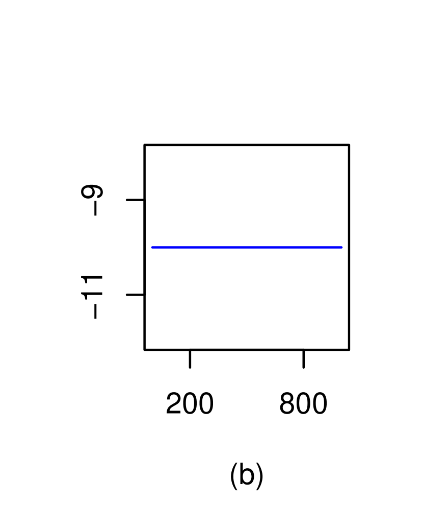
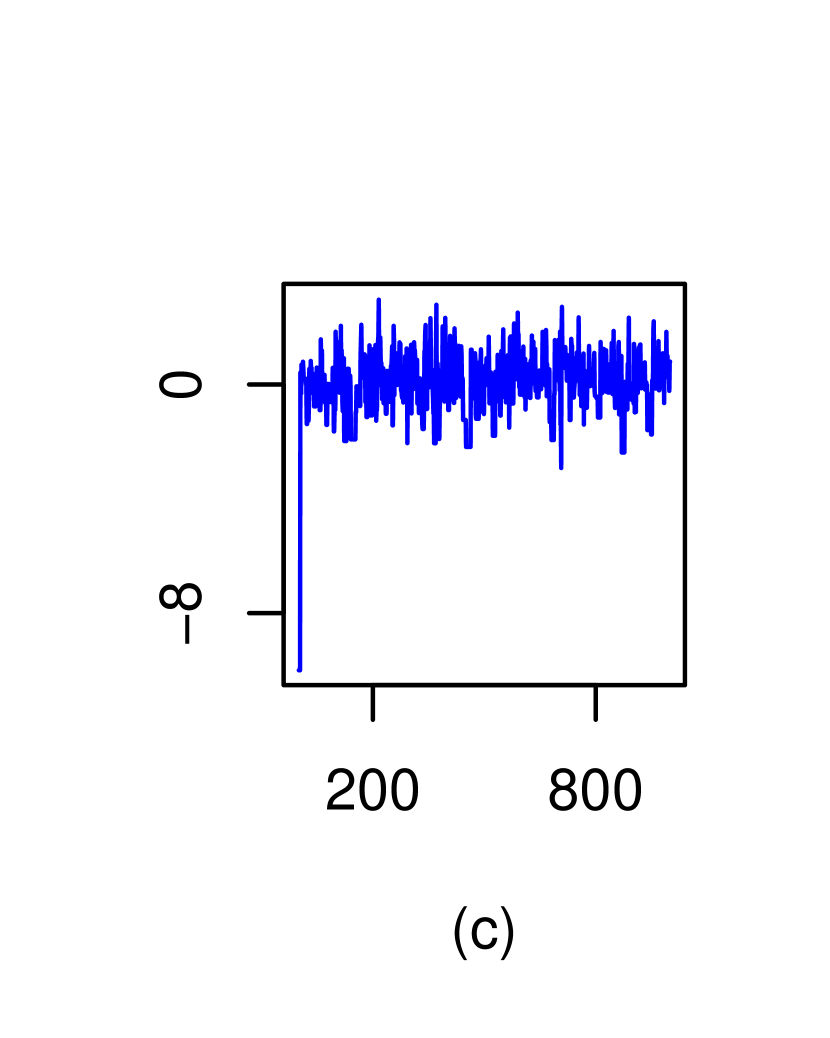
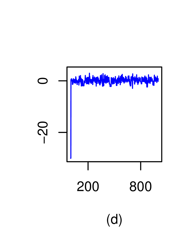
Figure 3: Trace plots for one thousand iterations of the independence Metropolis chains (a) starting at -5, (b) starting at -10, and of the manifold MH chains (c) starting at -10, (d) starting at -30 for the standard normal target.

From (17) and Mengersen and Tweedie (1996), we know that the independent MH chain is not geometrically ergodic. Now, we will verify (14) for the geometric MH algorithm.

Since $\phi(x)=\cos^{2}(\epsilon\theta)f(x)+\sin^{2}(\epsilon\theta)h(x),$ from (18) we have

$$\frac{\phi(x)}{\psi(x)} =\cos^{2}(\epsilon\theta)\exp(x-1/2)+\frac{\sin^{2}(\epsilon\theta)}{1-\exp(-1/4)}\Big{(}1-\exp(-1/8)\exp(x/2-1/4)\Big{)}$$

$$=\frac{\sin^{2}(\epsilon\theta)}{1-\exp(-1/4)}+r(x),$$

where $r(x)=\cos^{2}(\epsilon\theta)\exp(x-1/2)-[\sin^{2}(\epsilon\theta)\exp(-1/8)/\{1-\exp(-1/4)\}]\exp(x/2-1/4)$. It can be shown that $r(x)$ attains minimum at $c_{0}=2\log(\sin^{2}(\epsilon\theta)\exp(-1/8)/[2\cos^{2}(\epsilon\theta)\\ \{1-\exp(-1/4)\}])+1/2$. Thus,

$$\min_{x}\frac{\phi(x)}{\psi(x)} =\frac{\sin^{2}(\epsilon\theta)}{1-\exp(-1/4)}+r(c_{0})$$

$$=\frac{\sin^{2}(\epsilon\theta)}{1-\exp(-1/4)}-\frac{\sin^{4}(\epsilon\theta)\exp(-1/4)}{4\cos^{2}(\epsilon\theta)\{1-\exp(-1/4)\}^{2}},$$

which is positive for $\epsilon>0$. Thus, by Proposition 2, the geometric MH algorithm is uniformly ergodic in this example.

Example 2 (Random walk MH for Cauchy (0, 1) target).

Let the target density $\psi$ be the Cauchy $(0,1)$ density. We first consider the RWM chain with the increment $I\sim$ N $(0,1)$. From Jarner and Tweedie (2003) we know this RWM chain is not geometrically ergodic. We ran this chain for ten thousand iterations, and the leftmost plot of Figure 4 reveals the slow mixing of the chain. A heavier-tailed proposal in RWM for the Cauchy target can lead to a polynomial rate of convergence (Jarner and Roberts, 2007). We ran the RWM chain with $t_{2}$ proposal for ten thousand iterations and the second from the left plot of Figure 4 shows the high lag autocorrelations of this chain.

Next, we consider our proposed Algorithm 1 with independent base density $f=t_{\kappa},$ the $t$ density with degrees of freedom $\kappa$. With the baseline density $f=t_{\kappa}$, we form the proposal density $\phi(x)=\cos^{2}(\epsilon\theta)f(x)+\sin^{2}(\epsilon\theta)h(x)$ by perturbing $f$ in the direction of the target density $g=\psi$. Since

$$h(x)=\frac{1}{1-\langle\sqrt{f},\sqrt{g}\rangle^{2}}\Bigg{(}\frac{1}{\sqrt{\pi(1+x^{2})}}-\langle\sqrt{f},\sqrt{g}\rangle\sqrt{\frac{\Gamma(\frac{\kappa+1}{2})}{\sqrt{\kappa}\Gamma(\frac{\kappa}{2})}}\sqrt{\frac{1+x^{2}}{(1+x^{2}/\kappa)^{(\kappa+1)/2}}}\Bigg{)}^{2},$$

with degrees of freedom $\kappa=2$, we have

$$h(x)=\frac{1}{1-\langle\sqrt{f},\sqrt{g}\rangle^{2}}\frac{1}{\pi(1+x^{2})}\Bigg{(}1-\langle\sqrt{f},\sqrt{g}\rangle\Big{(}\frac{\pi}{2}\Big{)}^{1/4}2^{3/4}\sqrt{\frac{1+x^{2}}{(2+x^{2})^{3/2}}}\Bigg{)}^{2}.$$ (19)

Now

$$\sup_{x}\Bigg{(}1-\langle\sqrt{f},\sqrt{g}\rangle\Big{(}\frac{\pi}{2}\Big{)}^{1/4}2^{3/4}\sqrt{\frac{1+x^{2}}{(2+x^{2})^{3/2}}}\Bigg{)}^{2}=1.$$

Thus, we can sample from $h$ by first drawing $X\sim$ Cauchy (0, 1) and then accepting it with probability $(1-\langle\sqrt{f},\sqrt{g}\rangle^{2})h(x)/g(x)$. Again, in this case, $1/(1-\langle\sqrt{f},\sqrt{g}\rangle^{2})=25.538<M=M_{i,x}=50.077$ implying that the sampler based on the representation (6) results in lower acceptance rates than the rejection sampler based on Cauchy $(0,1)$. On the other hand, with $\epsilon=0.5,\sin^{2}(\epsilon\theta)=0.0099,$ implying that a sample from $h$ is drawn less than 1% of the time while sampling from $\phi$. We ran the independent geometric MH algorithm with $f=t_{2}$ for 10,000 iterations with $\epsilon=0.5$ using (6) to sample from $h$. From plot (c) in Figure 4 we see that the independent geometric MH algorithm results in much lower autocorrelations than the random walk MH chains. By Proposition 2 we know that the independent MH chain with $f=t_{2}$ proposal is not geometrically ergodic as $\min_{x}f(x)/\psi(x)=0$. On the other hand, since

$$\min_{x}\frac{\phi(x)}{\psi(x)}=\sin^{2}(\epsilon\theta)\min_{x}\Bigg{(}1-\langle\sqrt{f},\sqrt{g}\rangle\Big{(}\frac{\pi}{2}\Big{)}^{1/4}2^{3/4}\sqrt{\frac{1+x^{2}}{(2+x^{2})^{3/2}}}\Bigg{)}^{2}>0$$

for any $\epsilon>0$, by Proposition 2, the independent geometric MH algorithm is uniformly ergodic with $t_{2}$ baseline density. Finally, we ran the geometric MH algorithm with baseline proposal density $f=N(x,1)$ (that is, the normal RWM proposal density) for 10,000 iterations with $\epsilon=0.5$ (plot (d) in Figure 4). Unlike the other MH chains, autocorrelations of the geometric MH chains drop down to (practically) zero by five lags, revealing their fast mixing properties.

Figure 4: Autocorrelation function plots of the (a) random walk chain with normal proposal, (b) random walk chain with $t_{2}$ proposal, (c) independent geometric MH chain with $t_{2}$ baseline density and (d) the geometric MH chain with $N(x,1)$ baseline density where $x$ is the current state of the Markov chain.

Example 3 (Mixture of bivariate normals).

Suppose the target density $\psi$ is $\psi(x)=\\ 0.5\phi_{2}(x;\mu_{1},\Sigma_{1})+0.5\phi_{2}(x;\mu_{2},\Sigma_{2})$, where $\mu_{1}=(0,0)^{\top}$, $\mu_{2}=(10,10)^{\top}$, $\Sigma_{1}=I$ and $\Sigma_{2}=2I$.

We ran the RWM chain with the normal proposal density with covariance matrix $2I$ started at $(5,5)^{\top}$ for $100,000$ iterations. The estimated acceptance rate is 42.14%. The first row in Table 1 provides the estimates of the means of the two coordinates, mean square Euclidean jump distance(MSJD), effective sample size (ESS) for the two coordinates separately, and multivariate ESS (mESS) based on this RWM chain. The MSJD for a Markov chain $\{X^{(n)}\}_{n\geq 1}$ is defined as $\sum_{i=2}^{n+1}\|X^{(i)}-X^{(i-1)}\|^{2}/n$. We use the R package mcmcse (Flegal et al., 2021) for computing ESS and mESS values. The mean estimates are far from the true value $(5,5)$. The reason is that the random chain failed to move out of the local mode at $(0,0)$ even after $100,000$ iterations. The left panel of Figure 5 shows only the first 1000 steps of the chain.

We then ran the proposed geometric random walk chain with the same baseline density as the random walk MH chain for $100,000$ iterations initialized at $(5,5)^{\top}$. In this case, we took $k=2$, $g_{1}(y)\equiv\phi_{2}(y;\mu_{1},\Sigma_{1})$ and $g_{2}(y)\equiv\phi_{2}(y;\mu_{2},\Sigma_{2})$. Thus, $\mathcal{G}=\{g_{1},g_{2}\}$ is a set of two unimodal densities centered at the different local modes. Note that since $f(y|x)=\phi_{2}(y;x,2I)$, $\langle\sqrt{f},\sqrt{g_{i}}\rangle,i=1,2$ are available in closed form. From the middle panel of Figure 5, which shows the first 1000 steps of the geometric chain, we see that the chain can move back and forth between the two modes. Table 1 shows that the geometric chain (GMC1(RW)) results in higher ESS values and much higher MSJD, demonstrating better mixing.

Next, we consider the geometric random walk chain with the same baseline density $f$ as the RWM chain but $k=1$ and $g=\psi$. In this case, $\langle\sqrt{f},\sqrt{g}\rangle$ is not available in closed form and needs to be estimated. We estimate it by importance sampling using samples from $f$. The results from $100,000$ iterations of this chain (GMC2(RW)) initialized at $(5,5)^{\top}$ are given in Table 1. From these results, we see that GMC2(RW) performs better than the GMC1(RW) chain.

Finally, we ran a geometric Markov chain (GMC3(RW)) with the same base random walk proposal density $\phi_{2}(y;x,2I),$ but with a ‘non-informative’ choice of $g$, namely $g(y)=\phi_{2}(y;0,30^{2}I)$, a normal density centered at $0$ with covariance matrix $900I$. From Figure 5, we see that even with this choice of a diffuse density for $g$, the geometric MH chain successfully moves between the two local modes, resulting in estimates of the means close to their true values. On the other hand, unlike GMC1 and GMC2, GMC3 takes more time to move between the modes, resulting in lower MSJD values than GMC1 and GMC2. Note that the mESS for a Markov chain sample of size $n$ is defined as $n\sqrt{|\Lambda|/|\Sigma|}$ where $\Lambda$ is the sample covariance matrix and $\Sigma$ is an estimate of the Monte Carlo covariance matrix. Since the RW chain is stuck in a local mode, it is fooled into treating the target distribution as unimodal, and it results in small values of $|\Lambda|$ and $|\Sigma|$ leading to a higher value of mESS than that of GMC3 (Roy, 2020).

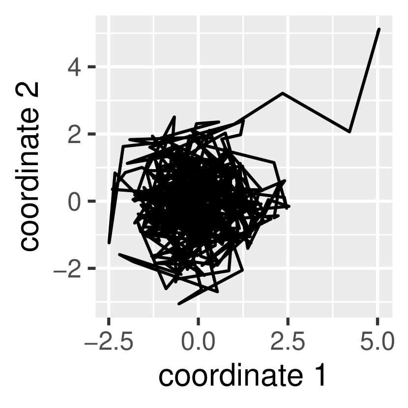
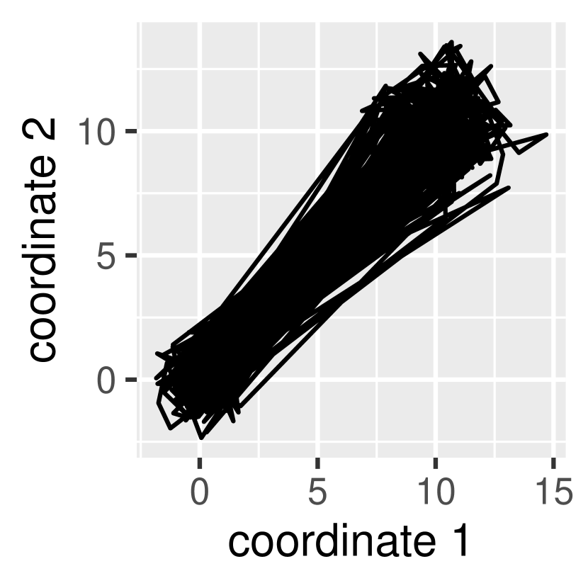
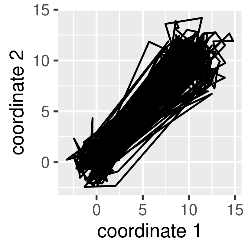
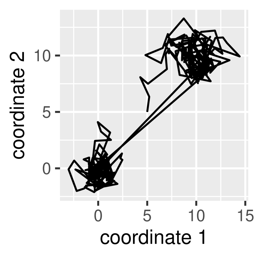
Figure 5: Illustration of trajectories for a mixture of two normals. The trajectory of the first 1000 iterations of different chains. The random walk chain (left plot) entirely lies in one mode, whereas the first geometric MH chain (second plot from the left), the second geometric MH chain (third plot from the left) and the third geometric MH chain (rightmost plot) with $N_{2}(x,2I)$ baseline density successfully move between the modes where $x$ is the current state of the Markov chain.

Next, we compare the three chains in terms of computational time. For completing $100,000$ iterations, the RW chain took around 10 seconds on an old Intel i7-870 2.93 GHz machine running Windows 10 with 16 GB RAM, whereas the GMC1(RW), GMC2(RW) and GMC3(RW) chains took a little less than two minutes, about 20 minutes, and about one minute, respectively. The extra time required in GMC2(RW) is due to computation of $\langle\sqrt{f},\sqrt{g}\rangle$ by importance sampling in every iteration of the Markov chain.

Table 1: Results for different samplers for the mixture model example

Sampler	$E(X_{1})$	$E(X_{2})$	MSJD	mESS	ESS $(X_{1})$	ESS $(X_{2})$
RW	-0.004	-0.004	0.916	11911	12224	11437
GMC1(RW)	- 6.729	- 6.721	29.586	17520	15132	15549
GMC2(RW)	- 5.025	- 5.035	33.352	23740	20371	18756
GMC3(RW)	- 4.675	- 4.705	0.957	1152	16578	17133

Example 4 (Bayesian logistic model).

We consider the Binary logistic regression model. Suppose $z=(z_{1},z_{2},\dots,z_{m})$ are $m$ independent observations where $z_{i}$ is either $0$ or $1$ and assume that $Z_{i}\sim\mbox{Ber}(\xi_{i})\ ,$ with $\log(\xi_{i}/[1-\xi_{i}])=w_{i}^{\top}\beta$ where $w_{i}$’s, $i=1,2,\dots,m$ are the $p\times 1$ covariate vectors and $\beta$ is the $p\times 1$ vector of regression coefficients. We consider the $p$-variate normal prior $N_{p}(\mu_{0},\Sigma_{0})$ with mean $\mu_{0}$ and covariance matrix $\Sigma_{0}$. Thus, the target posterior density is $\psi(\beta)\propto\bigg{[}\prod^{m}_{i=1}\frac{\exp(z_{i}w^{\top}_{i}\beta)}{1+\exp(w^{\top}_{i}\beta)}\bigg{]}\times\phi_{p}(\beta;\mu_{0},\Sigma_{0}).$

We consider the Pima Indian data set (Ripley, 1996). A population of women who were at least 21 years old, of Pima Indian heritage, and living near Phoenix, Arizona, was tested for diabetes, according to World Health Organization criteria. The data were collected by the US National Institute of Diabetes and Digestive and Kidney Diseases. We used the 532 complete records selected from a larger data set, with the binary observation denoting the presence or absence of diabetes, and $p=8$ covariates consisting of an intercept term and the following seven predictors: number of pregnancies, plasma glucose concentration in an oral glucose tolerance test, diastolic blood pressure (mm Hg), triceps skin fold thickness (mm), body mass index (weight in kg/$\mbox{(height in m)}^{2}$), diabetes pedigree function, and age (in years).

We analyze the Pima Indian data set by fitting a Bayesian logistic regression model using the RWM, independent MH algorithms, the MALA, the MMALA, and their geometric MH variants. We take $\mu_{0}=0_{8}$, a vector of zeros, and $\Sigma_{0}=10^{3}I_{8}$ for the prior density of $\beta$. We ran the algorithms for 100,000 iterations all started at $\mu_{0}$. Let $\hat{\beta}$ be the MLE of $\beta$. We obtain $\hat{\beta}$ by fitting the glm function of R with the logit link. Let $\hat{\Sigma}=(-\nabla^{2}\log\psi(\beta))^{-1}|_{\beta=\hat{\beta}}$, the generalized observed Fisher information matrix. For the RWM, we use a normal proposal with covariance matrix $\Sigma_{f}=0.3\hat{\Sigma}$ to get an acceptance rate of around 50%. For the independent MH, we use a normal proposal with mean $\hat{\beta}$ and covariance matrix $\hat{\Sigma}$ resulting in an acceptance rate of around 80%. For constructing MALA and MMALA, we need the first and higher-order derivatives of the log target density $\psi$. Indeed, the proposal density of MALA is $\phi(\beta^{\prime};\beta+h\nabla\log\psi(\beta)/2,hI_{d})$ for some step-size $h$ and $\beta$ is the current state of the Markov chain. It turns out that $\nabla\log\psi(\beta)=W^{\top}(z-\xi)-\Sigma_{0}^{-1}(\beta-\mu_{0}),\nabla^{2}\log\psi(\beta)=-W^{\top}\Lambda W-\Sigma_{0}^{-1}$ and $\frac{\partial\nabla^{2}\log\psi(\beta)}{\partial\beta_{j}}=-W^{\top}\Gamma^{j}X$, where $W$ is the $m\times p$ matrix of covariates, $\xi=(\xi_{1},\dots,\xi_{m})$, $\Lambda$ is the $m\times m$ diagonal matrix with $i$th diagonal element $\xi_{i}(1-\xi_{i}),i=1,\dots,m$, and $\Gamma^{j}$ is the $m\times m$ diagonal matrix with $i$th diagonal element $\xi_{i}(1-\xi_{i})(1-2\xi_{i})w_{ij},i=1,\dots,m$. For MALA and MMALA we take $h=0.01$ and $h=2$, respectively resulting in around 50% acceptance rates.

For the geometric variants of the above-mentioned RW and independent MH algorithms, we take $k=1$ and $g(\beta)=\phi_{p}(\beta;\hat{\beta},\hat{\Sigma})$. For the independent geometric chain (GMC(Ind)), we first consider $f(\beta)=\phi(\beta;\mu_{0},\Sigma_{f})$, although later we discuss another choice. In this case, $\langle\sqrt{f},\sqrt{g}\rangle=\langle\sqrt{\phi(\beta;\mu_{0},\Sigma_{f})},\sqrt{g}\rangle\approx\pi/2$, and thus $M\equiv M_{i,\beta}\approx 1$ where $M_{i,\beta}$ is defined in Section 6. On the other hand, for the RW geometric chain (GMC(RW)), $\langle\sqrt{f},\sqrt{g}\rangle$ needs to be computed in every iteration. Since the chains are started at $\mu_{0}$, for the first iteration, the value of $\langle\sqrt{f},\sqrt{g}\rangle$ will be the same as that of the independent geometric chain. If the mean of $f$ is $\hat{\beta}$, then $\langle\sqrt{\phi(\beta;\hat{\beta},\Sigma_{f})},\sqrt{g}\rangle=1.042$, and in that case $M=1.682$ giving around 60% acceptance probability for the sampling algorithm described in Section 6. Similarly, we consider geometric variants of MALA (GMC(MALA)) and MMALA (GMC(MMALA)). Table 2 provides ESS, mESS, their time normalized values, and MSJD values for the different samplers. For ESS, we provide the minimum, median, and maximum of the eight values corresponding to $p=8$ covariates. Table 3 shows the first eight autocorrelations for the function $\beta^{\top}W^{\top}W\beta$ for the different Markov chains. The function $\beta^{\top}W\beta$ is a natural choice as it is used as the drift function to prove the geometric ergodicity of some Gibbs samplers for some Bayesian binary regression models (see e.g Roy and Hobert, 2007). GMC(MMALA) has superior performance over the other algorithms in terms of ESS and autocorrelation, closely followed by the independent MH algorithm. On the other hand, in terms of the time-normalized values, the independent MH algorithm with the proposal $g$ beats all other algorithms. Next, we consider the independent MH algorithm with a proposal $f_{1}(\beta)=\phi_{p}(\beta;\mu_{0},${10}^{-6}$I_{8})$. This algorithm (Ind ($f_{1}$)) results in small ESS and MSJD values and large autocorrelations. Thus, the independent MH algorithm’s performance suffers greatly with the proposal density change. On the other hand, the performance of the GMC (Ind) does not vary much when $f(\beta)=\phi(\beta;\mu_{0},\Sigma_{f})$ is replaced with $f_{1}(\beta)$. Finally, we consider the geometric RW algorithm (GMC(RW ($f_{1}$))) with a ‘non-informative’ choice for $g$, namely $g=f_{1}$. From Tables 2 and 3, we see that this algorithm performs similarly to the original GMC (RW). For the geometric variants of the algorithms, we did not choose the step size or the variance of the baseline densities, optimizing their empirical performance; we used $\epsilon=0.5$ and other values the same as the non-geometric chains. By changing $\epsilon$, geometric algorithms’ acceptance rate and performance can greatly vary. For example, the GMC(RW) chain in Table 2 with $\epsilon=0.5$ has 62% acceptance rate, whereas for $\epsilon=0.1$ and $0.9$, it results in 45% and 83% acceptance rates, respectively.

Table 2: Multivariate ESS and ESS (minimum, median, maximum) and their time normalized values for different samplers for the Pima Indian data

Sampler	mESS	ESS	mESS/sec	ESS/sec	MSJD
RW	2765	(2405,2833,3155)	45	(39,46,51)	0.019
GMC(RW)	22460	(18094,21210,23873)	158	(127,149,167)	0.123
Ind	56782	(42972,59874,62279)	745	(564,786,818)	0.263
GMC(Ind)	21405	(19266,21078,23126)	180	(162,177,195)	0.131
Ind($f_{1}$)	77	(32,72,83)	0.97	(0,1,1)	2.7e-7
GMC(Ind ($f_{1}$))	21406	(19263,21078,23125)	174	(157,172,188)	0.131
GMC(RW ($f_{1}$))	24682	(21289,25674,27640)	172	(149,179,193)	0.142
MALA	10948	(4953,7473,12245)	120	(54,82,134)	0.033
GMC(MALA)	28386	(20963,22638,26727)	101	(74,80,95)	0.133
MMALA	35032	(33070,34381,36491)	57	(54,56,59)	0.136
GMC(MMALA)	58160	(51354,59985,61494)	15	(13,15,16)	0.248

Table 3: First eight autocorrelations for different samplers applied to the Pima Indian data

Sampler	lag1	lag2	lag3	lag4	lag5	lag6	lag7	lag8
RW	0.941	0.886	0.835	0.787	0.742	0.699	0.658	0.620
GMC(RW)	0.663	0.452	0.314	0.223	0.162	0.122	0.096	0.078
Ind	0.313	0.143	0.082	0.059	0.044	0.037	0.028	0.021
GMC(Ind)	0.657	0.446	0.310	0.221	0.164	0.126	0.098	0.079
Ind($f_{1}$)	0.997	0.995	0.993	0.991	0.989	0.987	0.985	0.984
GMC(Ind ($f_{1}$))	0.657	0.446	0.310	0.221	0.164	0.126	0.098	0.079
GMC(RW ($f_{1}$))	0.622	0.401	0.268	0.186	0.130	0.096	0.071	0.056
MALA	0.784	0.630	0.514	0.426	0.356	0.300	0.252	0.209
GMC(MALA)	0.603	0.379	0.243	0.161	0.108	0.073	0.051	0.038
MMALA	0.440	0.238	0.142	0.097	0.068	0.046	0.032	0.021
GMC(MMALA)	0.342	0.130	0.053	0.0267	0.018	0.016	0.008	0.006

Example 5 (Bayesian variable selection).

We now consider the so-called variable selection problem, where we have a $m\times 1$ vector of response values $z=(z_{1},\ldots,z_{m})$, a $m\times p$ design matrix $W=(W_{1},\ldots,W_{p})$ with each column of $W$ representing a potential predictor and the goal is to identify the set of all important covariates which have non-negligible effects on the response $z$. In a typical GWAS, the number of markers, $p$ far exceeds the number of observations $m$, although only a few of these variables are believed to be associated with the response. Here, we consider a popular approach to variable selection (Mitchell and Beauchamp, 1988; George and McCulloch, 1993, 1997; Narisetty and He, 2014; Li et al., 2023) based on a Bayesian hierarchical model mentioned below.

Let $\beta$ denote the $p$ dimensional vector of regression coefficients, $\gamma$ denote a subset of $\{1,2,\dots,p\}$ and the cardinality of $\gamma$ be denoted by $|\gamma|$. Corresponding to a given model $\gamma$, let $W_{\gamma}$ denote the $n\times|\gamma|$ sub-matrix of $W$ and $\beta_{\gamma}$ denotes the $|\gamma|$ dimensional sub-vector of $\beta$ . Let $1_{m}$ denotes a $m$-vector of 1’s. The Bayesian hierarchical regression model we consider is given by

$$z|\beta,\beta_{0},\sigma^{2},\gamma \sim N_{m}\left(1_{m}\beta_{0}+W_{\gamma}\beta_{\gamma},\sigma^{2}I\right),$$ (20a)

$$\beta_{j}|\beta_{0},\sigma^{2},\gamma \stackrel{{\scriptstyle\text{ ind }}}{{\sim}}N\left(0,\frac{\gamma_{j}}{\lambda}\sigma^{2}\right)\text{ for }j=1,\ldots,p,$$ (20b)

$$\left(\beta_{0},\sigma^{2}\right)|\gamma \sim 1/\sigma^{2},$$ (20c)

$$\gamma|\omega \sim\omega^{|\gamma|}(1-\omega)^{p-|\gamma|}.$$ (20d)

In the model (20), (20a) indicates that conditional on the parameters, each $\gamma$ corresponds to a Gaussian linear regression model $z=\beta_{0}1_{m}+W_{\gamma}\beta_{\gamma}+\epsilon$ where the residual vector $\epsilon\sim N_{m}(0,\sigma^{2}I).$ Given $\gamma$, a popular non-informative prior is set for $(\beta_{0},\sigma^{2})$ in (20c) and a conjugate independent normal prior is used on $\beta$ in (20b) with the common parameter $\lambda>0$ controlling the precision of the prior. Following the common practice, here, we assume that the covariate matrix $W$ is scaled. Note that, if a covariate is not included in the model, the prior on the corresponding regression coefficient degenerates at zero. The prior of $\gamma$ in (20d) is obtained by assuming independent Bernoulli distribution for each indicator variable indicating the presence or absence of variables corresponding to the model and $\omega\in(0,1)$ is the prior inclusion probability of each predictor. The hyperparameters $\lambda$ and $\omega$ are assumed known (see Narisetty and He, 2014; Li et al., 2023, for appropriate choices of these parameters.).

It is possible to analytically integrate out $\beta_{0},$ $\beta_{\gamma}$ and $\sigma^{2}$ from the hierarchical model (20), and the marginal posterior pmf of $\gamma$ is given by

$$\psi(\gamma|z)\propto\lambda^{|\gamma|/2}|A_{\gamma}|^{-1/2}R_{\gamma}^{-(m-1)/2}\omega^{|\gamma|}(1-\omega)^{p-|\gamma|},$$ (21)

where $A_{\gamma}=W_{\gamma}^{\top}W_{\gamma}+\lambda I,$ $|A_{\gamma}|$ is the determinant of $A_{\gamma},R_{\gamma}=\tilde{z}^{\top}\tilde{z}-\tilde{z}^{\top}W_{\gamma}A_{\gamma}^{-1}W_{\gamma}^{\top}\tilde{z}$ is the ridge residual sum of squares, and $\tilde{z}=z-\bar{z}1_{m}$ with $\bar{z}=\sum_{i=1}^{m}z_{i}/m.$ The density (21) is usually explored by MCMC sampling and several MH and Gibbs algorithms have been proposed in the literature (see e.g George and McCulloch, 1997; Guan and Stephens, 2011; Yang et al., 2016; Griffin et al., 2021; Zanella and Roberts, 2019; Zhou et al., 2022; Liang et al., 2022). The proposal densities of MH algorithms for (21) are generally mixtures of three types of local moves, namely “addition”, “deletion” and “swap”. In order to describe these proposals, for a given model $\gamma$, let $\mathcal{N}(\gamma)=\gamma^{+}\cup\gamma^{\circ}\cup\gamma^{-}$ denote a neighborhood of $\gamma$, where $\gamma^{+}$ is an “addition” set containing all the models with one of the $p-|\gamma|$ remaining covariates added to the current model $\gamma$, $\gamma^{-}$is a “deletion” set obtained by removing one variable from $\gamma;$ and $\gamma^{\circ}$ is a “swap” set containing the models with one of the variables from $\gamma$ replaced by one variable from $\gamma^{c}.$ The proposal densities of the MH chains are of the form

$$f(\gamma^{\prime}|\gamma)=\frac{b^{+}(\gamma)I_{\gamma^{+}}(\gamma^{\prime})}{p-|\gamma|}+\frac{b^{-}(\gamma)I_{\gamma^{-}}(\gamma^{\prime})}{|\gamma|}+\frac{b^{\circ}(\gamma)I_{\gamma^{\circ}}(\gamma^{\prime})}{|\gamma|(p-|\gamma|)},$$ (22)

where $b^{+}(\gamma),b^{-}(\gamma),b^{\circ}(\gamma)$ are non-negative constants summing to 1. When $b^{+}(\gamma),b^{-}(\gamma),b^{\circ}(\gamma)$ are all constants independent of $\gamma$, Zhou et al. (2022) refer to the resulting MH algorithm as asymmetric RW. In their simulation examples, Zhou et al. (2022) sets $b^{+}(\gamma)=b^{-}(\gamma)=0.4,b^{\circ}(\gamma)=0.2$. Yang et al. (2016) set $b^{+}(\gamma)=(p-|\gamma|)/2p,b^{-}(\gamma)=|\gamma|/2p$ and $b^{\circ}(\gamma)=1/2$, and since in this case, $f(\gamma^{\prime}|\gamma)=f(\gamma|\gamma^{\prime})$ for all $\gamma,\gamma^{\prime}$, the resulting MH algorithm is called the symmetric RW. Yang et al. (2016) establish rapid mixing (mixing time is polynomial in $m$ and $p$) of the symmetric RW algorithm, but in high dimensional examples, the RW algorithms can suffer from slow convergence, and their efficiency can be improved by using informative proposals. Indeed, motivated by Zanella (2020), where variable selection was not discussed explicitly, a couple of other informative proposals have recently been constructed, for example, the tempered Gibbs sampler of Zanella and Roberts (2019), the adaptively scaled individual adaptation proposal of Griffin et al. (2021), and the Locally Informed and Thresholded proposal distribution of Zhou et al. (2022).

We now consider our proposed geometric MH algorithm with $k=1$, the base density (22) and

$$g(\gamma^{\prime}|\gamma)=\begin{cases}\frac{\psi(\gamma|z)}{c_{\gamma}}&\text{ if }\gamma^{\prime}\in\mathcal{N}(\gamma),\\ 0,&\text{otherwise},\end{cases}$$ (23)

where $c_{\gamma}=\sum_{\gamma^{\prime}\in\mathcal{N}(\gamma)}\psi(\gamma|z)$. For implementing this proposed algorithm, we need to efficiently compute $\psi(\gamma|z)$ for all $\gamma^{\prime}\in\mathcal{N}(\gamma)$. Note that Zhou et al. (2022) consider only the ‘addition’ and ‘deletion’ moves in their simulation examples, greatly reducing the computational burden. Here, we use the fast Cholesky updates of Li et al. (2023) for rapidly computing $\psi(\gamma|z)$ for all $\gamma^{\prime}\in\mathcal{N}(\gamma)$. Furthermore, both Yang et al. (2016) and Zhou et al. (2022) use Zellner’s (1986) $g-$prior on $\beta$ and a different prior on $\gamma$. The $g-$prior, although a popular alternative to the independent normal prior (20b), it requires all $m\times q$ sub-matrices of $W$ have full column rank for $q\leq m-1$ and the support of the prior on $\gamma$ is restricted to models of size at most $m-1$.

We now perform extensive simulation studies and compare our geometric MH algorithm to the RW algorithms. In particular, we consider the symmetric RW (RW1), the asymmetric RW with $b^{+}(\gamma)=b^{-}(\gamma)=0.4,b^{\circ}(\gamma)=0.2$ (RW2), the two geometric MH algorithms with the base density (22) corresponding to RW1 and RW2, denoted by GMC1 and GMC2, respectively. Our numerical studies are conducted in the following five different simulation settings.

Independent predictors: In this example, following Li et al. (2023), entries of $W$ are generated independently from $N(0,1)$. The coefficients are specified as $\beta_{1}=0.5,\beta_{2}=0.75,\beta_{3}=1,\beta_{4}=1.25,\beta_{5}=1.5,$ and $\beta_{j}=0,\forall j>5.$

Compound symmetry: This example is taken from Example 2 in Wang and Leng (2016). The rows of $W$ are generated independently from $N_{p}\left(0,(1-\rho)I_{p}+\rho 1_{p}1_{p}^{\top}\right)$ where we take $\rho=0.6$. The regression coefficients are set as $\beta_{j}=5$ for $j=1,\ldots,5$ and $\beta_{j}=0$ otherwise.

Auto-regressive correlation: Following Example 2 in Wang and Leng (2016), $W_{j}=\rho W_{j-1}+(1-\rho^{2})^{1/2}b_{j},$ for $1\leq j\leq p,$ where $W_{0}$ and $b_{j}$ ($1\leq j\leq p)$ are iid $\sim N_{m}(0,I_{m}).$ Following Li et al. (2023), we use $\rho=0.6$ and set the regression coefficients as $\beta_{1}=3$, $\beta_{4}=1.5$, $\beta_{7}=2$ and $\beta_{j}=0$ for $j\not\in\{1,4,7\}$.

Factor models: Following Wang and Leng (2016) and Li et al. (2023), we first generate a $p\times 2$ factor matrix $F$ whose entries are iid standard normal. Then the rows of $W$ are independently generated from $N_{p}(0,FF^{\top}+I_{p}).$ The regression coefficients are set to be the same as in compound symmetry example.

Extreme correlation: Following Wang and Leng (2016), in this challenging example, we first simulate $b_{j}$ , $j=1,\ldots,p$ and $t_{j}$, $j=1,\ldots,5$ independently from $N_{m}(0,I_{m})$. Then the covariates are generated as $W_{j}=(b_{j}+t_{j})/\sqrt{2}$ for $j=1,\ldots,5$ and $W_{j}=(b_{j}+\sum_{i=1}^{5}t_{i})/2$ for $j=6,\ldots,p$. As in Li et al. (2023), we set $\beta_{j}=5$ for $j=1,\ldots,5$ and $\beta_{j}=0$ for $j=6,\dots,p$. Thus, the correlation between the response and the unimportant covariates is around $2.5/\sqrt{3}$ times larger than that between the response and the true covariates, making it difficult to identify the important covariates.

Our simulation experiments are conducted using 100 simulated pairs of training and testing datasets. For each simulation setting, we set $p=10000$ and $m=400$ for both training and testing data sets. Following Li et al. (2023), we choose $w$ and $\lambda$ to be $\sqrt{m}/p$ and $m/p^{2}$, respectively. The error variance $\sigma^{2}$ is set by assuming different theoretical $R^{2}$ values. While the results for $R^{2}=90\%$ are provided in Table 4, the Appendix B contains the results for $R^{2}=60\%$ and $R^{2}=75\%$. All results are based on 100 iterations of the GMC chains and 50,000 iterations of the RW chains with all chains started at the null model.

To evaluate the performance of the MCMC algorithms, we consider several metrics that we describe now. Following Zhou et al. (2022), let $\hat{\gamma}_{\text{max}}$ be the model with the largest posterior probability that has been sampled by any of the four algorithms. If an algorithm has never sampled $\hat{\gamma}_{\text{max}}$, the run is considered as a failure. Also, let $\hat{\gamma}_{\text{med}}$ be the median probability model, that is, $\hat{\gamma}_{\text{med}}$ is the set of variables with estimated marginal inclusion probability (MIP) above 0.5 (Barbieri et al., 2004). We compute (1) Number of runs (Success) out of 100 repetitions when $\hat{\gamma}_{\text{max}}$ is sampled (2) median number of iterations ($N_{\text{success}}$) needed to sample $\hat{\gamma}_{\text{max}}$ among the successful runs (3) median time in seconds (Time) to reach $N_{\text{success}}$ among the successful runs (4) mean squared prediction error (MSPE) based on $\hat{\gamma}_{\text{med}}$ for testing data (5) mean squared error (MSE_β) between the estimated regression coefficients corresponding to $\hat{\gamma}_{\text{med}}$ and the true coefficients (6) average model size (size), which is calculated as the average number of predictors included in $\hat{\gamma}_{\text{med}}$ overall the replications (7) coverage probability (coverage) which is defined as the proportion of times $\hat{\gamma}_{\text{med}}$ contains the true model (8) false discovery rate (FDR) for $\hat{\gamma}_{\text{med}}$ (9) false negative rate (FNR) for $\hat{\gamma}_{\text{med}}$ and (10) the Jaccard index, which is defined as the size of the intersection divided by the size of the union of $\hat{\gamma}_{\text{med}}$ and the true model. All computations for these simulation examples are done on the machine mentioned in Example 3.

Table 4: Results for different samplers for the Bayesian variable selection example. Success, Coverage, FDR, FNR and Jaccard Index are reported in percentages.

	Success	$N_{\text{success}}$	Time	MSPE	MSEβ	Model size	Coverage	FDR	FNR	Jaccard Index
	Independent design
RW1	64	32458	126.89	1.803	1.192	3.42	19	0.0	31.6	68.4
GMC1	100	9	0.92	0.636	0.008	5.00	100	0.0	0.0	100.0
RW2	49	31849	120.45	2.224	1.570	3.20	11	0.0	36.0	64.0
GMC2	100	10	0.97	0.636	0.008	5.00	100	0.0	0.0	100.0
	Compound symmetry design with $r=0.6$
RW1	56	36126	213.50	56.998	22.450	4.39	50	0.7	12.8	86.8
GMC1	100	9	0.92	48.149	1.366	5.00	100	0	0.0	100.0
RW2	62	27286	141.17	70.738	51.577	3.84	28	3.3	26.0	72.9
GMC2	100	10	0.98	48.149	1.366	5.00	100	0	0.0	100.0
	Autoregressive correlation design with $r=0.6$
RW1	62	31092	126.58	3.433	1.855	2.79	64	6.7	13.3	83.6
GMC1	100	6	0.47	2.148	0.021	3.01	100	0.2	0.0	99.8
RW2	82	24836	94.07	4.790	3.866	2.65	45	11.3	22.3	73.6
GMC2	100	6	0.44	2.148	0.021	3.01	100	0.2	0.0	99.8
	Factor model design
RW1	54	34870	175.73	79.107	30.563	4.11	33	1.8	19.6	79.5
GMC1	99	11	1.12	43.014	1.338	4.96	99	0.0	0.8	99.2
RW2	61	35321	162.96	102.566	49.133	3.52	13	2.2	31.4	67.6
GMC2	100	10	0.97	42.005	0.328	5.00	100	0.0	0.0	100.0
	Extreme correlation design
RW1	47	35036	171.90	39.850	27.131	4.02	36	1.4	20.8	78.5
GMC1	100	12	1.22	16.968	6.563	4.85	96	3.5	3.8	96.2
RW2	58	31982	145.68	48.720	37.798	3.70	19	3.1	28.4	70.3
GMC2	100	11	1.07	14.182	0.178	5.00	100	0.0	0.0	100.0

From Table 4, we see that the proposed geometric algorithms successfully find the model $\hat{\gamma}_{\text{max}}$ in all 100 repetitions across all five simulation settings. Whereas the RW algorithms failed to find $\hat{\gamma}_{\text{max}}$ around $40\%$ of the time, and the failure rate could be as high as $53\%$. Also, across all three different values of $R^{2}$, we see that the proposed geometric algorithms always hit $\hat{\gamma}_{\text{max}}$ much faster than the RW algorithms. Indeed, remarkably, starting from the null model, the median number of iterations ($N_{\text{success}}$) to reach the model $\hat{\gamma}_{\text{max}}$ for the informative MH algorithms is always less than 15, except for the extreme correlation design with $R^{2}=75\%$ when $N_{\text{success}}=25$ for GMC1. On the other hand, among the successful runs, RW algorithms generally required about 30,000 iterations to find $\hat{\gamma}_{\text{max}}$. From Table 4, we see that the median wall time needed for the geometric MH algorithms to generate $N_{\text{success}}$ samples is less than 1.3 seconds in all five scenarios, whereas, among the successful runs, the average time to reach $\hat{\gamma}_{\text{max}}$ for the RW algorithms was as high as 3.5 minutes. Also, model averaging with 100 samples of the geometric MH algorithms results in much better performance than for the RW algorithms with 50,000 iterations. Indeed, the median probability model $\hat{\gamma}_{\text{med}}$ obtained from the informed MH algorithms is generally the true model leading to about 100% coverage. Also, the geometric MH algorithms resulted in larger Jaccard index values and smaller MSPE and MSE_β values. Also, although the symmetric RW generally outperformed the asymmetric RW, the geometric MH algorithms based on either of these RW algorithms resulted in similar performance. Thus, the GMC algorithms outperform the RW algorithms in terms of finding the maximum a posteriori model $\hat{\gamma}_{\text{max}}$, as well as leading to better model fitting and prediction accuracies based on Bayesian model averaging.

Real data analysis: We now consider an ultra-high dimensional real dataset and analyze it by fitting (20) using the proposed geometric MH algorithm. This maize shoot apical meristem (SAM) dataset was generated by Leiboff et al. (2015). The maize SAM is a small pool of stem cells that generate all the above-ground organs of maize plants. Leiboff et al. (2015) showed that SAM size is correlated with a variety of agronomically important adult traits such as flowering time, stem size, and leaf node number. In Leiboff et al. (2015), a diverse panel of 369 maize inbred lines was considered, and close to 1.2 million single nucleotide polymorphisms (SNPs) were used to study the SAM volume. After removing duplicates and SNPs with minor allele frequency (MAF) less than 5%, we end up with $p=810,396$ markers, and the response $z$ is the log of the SAM volume for $m=369$ varieties. The inbred varieties are bi-allelic, and we store the marker information in a sparse format by coding the minor alleles by one and the major alleles by zero.

We first ran the GMC1 chain with $\lambda=m/p^{2}=5.61865e-$10 and $w=\sqrt{m}/p=2.37037e-$5 (the default choices for $\lambda$ and $w$ in the function geomc.vs in the accompanying R package geommc) for $N=100$ iterations starting from the null model. Only one variable resulted in with estimated MIP above 0.5. Indeed, $\hat{\gamma}_{\text{med}}=1_{83878775}$. The $R^{2}$ value based on fitting $\hat{\gamma}_{\text{med}}$ on the response $z$ is 20.07%. Next, we ran the GMC1 chain for 100 iterations starting at the null model, but this time following Li et al. (2023), we took $\lambda=\sqrt{m}=19.20937$ (high shrinkage) and a higher value for $w=m/p=0.00046$. This time, $\hat{\gamma}_{\text{med}}$ contained four variables with $\hat{\gamma}_{\text{med}}=(1_{83878775},2_{175541357},3_{226820323},8_{27127525})$. In addition to the estimated median model $\hat{\gamma}_{\text{med}}$, we also consider a weighted average model (WAM) $\hat{\gamma}_{\text{wam}}$. For the unique MCMC samples $\{\gamma^{(n)}\}_{n=1}^{N}$ we assign the weights $\text{wt}_{n}=\psi(\gamma^{(n)}|z)/\sum_{i=1}^{N}\psi(\gamma^{(i)}|z)$ according to the marginal posterior pmf (21). Then, the approximate marginal inclusion probability for the $j$th variable is computed as $\hat{\pi}_{j}=\sum_{n=1}^{N}\text{wt}_{n}\mathbb{I}(\gamma^{(n)}_{j}=1)$ and define the WAM as the model containing variables $j$ with $\hat{\pi}_{j}>0.5.$ Based on the 100 iterations of the GMC1 chain, $\hat{\gamma}_{\text{wam}}$ consisted of five variables with $\hat{\gamma}_{\text{wam}}=(1_{83878775},2_{79769999},2_{175541357},8_{27127525},10_{10606917})$. The $R^{2}$ values for $\hat{\gamma}_{\text{med}}$ and $\hat{\gamma}_{\text{wam}}$ are 39.10% and 43.93%, respectively. We analyzed the real dataset on a Linux server equipped with 128 cores of AMD EPYC 7542 CPU and 1 TB of RAM, where it took 5.34 minutes to complete 100 iterations of GMC1 with $\lambda=\sqrt{m}$ and $w=m/p$. With these values of $(\lambda,w)$, we repeated 100 iterations of GMC1 50 times, each time with a different seed. The models $\hat{\gamma}_{\text{med}}$ and $\hat{\gamma}_{\text{wam}}$ vary in these 50 runs, suggesting that the posterior surface is highly multimodal. The range of the size of $\hat{\gamma}_{\text{med}}$ and $\hat{\gamma}_{\text{wam}}$ are (2,7) and (3, 9), respectively. Also, the ranges of $R^{2}$ values for $\hat{\gamma}_{\text{med}}$ and $\hat{\gamma}_{\text{wam}}$ are (27.29%, 46.85%) and (32.76%, 57.18%), respectively.

When we ran GMC2 for 100 iterations with $\lambda=m/p^{2}$ and $w=\sqrt{m}/p$ started at the null model, both $\hat{\gamma}_{\text{med}}$ and $\hat{\gamma}_{\text{wam}}$ resulted in the empty model, although the marker with the largest MIP and the largest weighted MIP was the same SNP $1_{83878775}$ obtained by GMC1 with these choices for $(\lambda,w)$. Indeed, the largest MIP and weighted MIP were 0.47 and 0.49, respectively. Next, we ran the GMC2 chain for 100 iterations started at the null model with $\lambda=\sqrt{m}$ and $w=m/p$. Based on the 100 iterations of the GMC2 chain, $\hat{\gamma}_{\text{med}}$ consisted of eight variables with $\hat{\gamma}_{\text{med}}=(1_{83878648},2_{175541342},2_{179751269},4_{225874150},5_{21046482},\\ 8_{14610995},8_{72384070},$ $8_{115299982})$ and $\hat{\gamma}_{\text{wam}}=(1_{83878648},2_{175541342},3_{170821024},4_{237392971},8_{72384070},\\ 9_{4338284})$. The $R^{2}$ values for $\hat{\gamma}_{\text{med}}$ and $\hat{\gamma}_{\text{wam}}$ in this case are 43.09% and 49.37%, respectively. It took 11.22 minutes to complete 100 iterations of GMC2 with $\lambda=\sqrt{m}$ and $w=m/p$. Finally, based on 50 repetitions of 100 iterations of the GMC2 chain with $\lambda=\sqrt{m}$ and $w=m/p$, each time with a different seed, we observe the ranges of the size of $\hat{\gamma}_{\text{med}}$ and $\hat{\gamma}_{\text{wam}}$ are (4,17) and (2, 8), respectively. Also, the ranges of $R^{2}$ values for $\hat{\gamma}_{\text{med}}$ and $\hat{\gamma}_{\text{wam}}$ are (40.11%, 60.10%) and (28.91%, 54.61%), respectively.

8 Discussion

In this work, we have proposed an original framework for developing informative MCMC schemes. The availability of explicit expressions for the exponential and inverse exponential maps under the novel use of square-root representation for pdfs plays a crucial role in constructing computationally efficient Riemannian manifold geometric MCMC algorithms. The Riemannian manifold MCMC algorithms available in the literature work for only continuous targets and involve heavy computational burden for evaluating the transition densities as well as for adjusting the tuning parameters. On the other hand, the proposed geometric MH algorithm works for both discrete and continuous targets, provides a simple step size tuning as in RWM based on acceptance rates criteria, and allows a flexible framework for using cheap to evaluate local and global approximations of the target to control the directions of moving the candidate density while still using the exact target density in the MH acceptance rate. Thus, the proposed method shows the utility of the explicit use of the intrinsic geometry of the space of pdfs in constructing informative MCMC schemes.

Analyses of different high dimensional linear, nonlinear, multimodal complex statistical models demonstrate the broad applicability of the proposed method. These examples using both real and simulated data show that the proposed geometric MCMC algorithms can lead to huge improvements in mixing and efficiency over alternative MCMC schemes. The empirical findings corroborate the theoretical results derived here, comparing the geometric MCMC with the MH chain using the base proposal density. The theoretical results developed here regarding different Markov chain orderings hold for general state space Markov chains and can be used to compare any MCMC algorithms.

The article presents various avenues for potential extensions and future methodological and theoretical works. The proposed geometric MCMC scheme is general and can be applied to sample from arbitrary discrete or continuous targets. The methodology is flexible and allows general choices for the baseline density and various local/global approximations of the target for specifying the directions of moving the baseline proposal density. For the popular Bayesian variable selection model considered here, we have developed some specific choices for the densities $f$ and $g$ and are implemented in the accompanying R package geommc. In particular, we have used RW base densities and the target pmf on a neighborhood as $g$. We have demonstrated the efficiency of the resulting geometric MH algorithm through analyses of high dimensional simulated datasets and a gigantic real dataset with close to a million markers for GWAS. One can consider the Locally Informed and Thresholded proposal of Zhou et al. (2022) and the adaptively scaled individual adaptation proposal of Griffin et al. (2021) as base densities. In particular, by allowing multiple variables to be added or deleted from the model in a single iteration, the algorithm can make large jumps in model space (Guan and Stephens, 2011; Liang et al., 2022). For $g$, one can consider various local tempered and non-tempered versions of $\psi$ (Zanella and Roberts, 2019). We anticipate future works exploring and comparing different choices of $\mathcal{G}$ mentioned in Section 3 and developing appropriate $f$ and $g$ functions for constructing efficient geometric MCMC schemes for other classes of statistical models.

Algorithm 1 uses a fixed $\epsilon$; on the other hand, one can choose $\epsilon$ adaptively, on the fly. A potential future work is to build such adaptive versions of Algorithm 1. Also, it will be interesting to study the performance of the geometric MH algorithm when used in a Metropolis-within-Gibbs framework. This will be useful in different settings, for example, when the Bayesian variable selection example in Section 3 is extended to handle ordinal responses (Zheng et al., 2023). Zhou et al. (2022) prove that the mixing time of LIT-MH is independent of the number of covariates under the assumptions of Yang et al. (2016). Zhou and Chang (2023) derived mixing time bounds for random walk MH algorithms for high-dimensional statistical models with discrete parameter spaces and more recently Chang and Zhou (2024) extended these results to study Zanella’s (2020) informed MH algorithms. A future study is to undertake such mixing time analysis of our proposed geometric MH algorithm for Bayesian variable selection.

Appendices

Appendix A An alternative geometric MH algorithm

We now describe an alternative to Algorithm 1. Denoting this alternative geometric MH chain by $\{\tilde{X}^{(n)}\}_{n\geq 1}$, suppose $\tilde{X}^{(n-1)}=x$ is the current value of the chain. The following iterations are used to move to $\tilde{X}^{(n)}$.

Algorithm 2 The $n$th iteration

1:  Choose $i^{\prime}\in\{1,\dots,k\}$ with probability $P(i^{\prime}=i)=a_{i},1\leq i\leq k$.

2:  Draw $y\sim\phi_{i^{\prime},\epsilon}(y|x)$.

3:  Set

$$\tilde{\alpha}_{i^{\prime}}(x,y)=\mbox{min}\Big{\{}\frac{\psi(y)\phi_{i^{\prime},\epsilon}(x|y)}{\psi(x)\phi_{i^{\prime},\epsilon}(y|x)},1\Big{\}}.$$ (24)

4:  Draw $\delta\sim$ Uniform $(0,1)$. If $\delta<\tilde{\alpha}_{i^{\prime}}(x,y)$ then set $\tilde{X}^{(n)}\leftarrow y$, else set $\tilde{X}^{(n)}\leftarrow x$.

Appendix B Further simulation results for the Bayesian variable selection example

This section presents the results for different simulation settings corresponding to $R^{2}=0.75$ and $R^{2}=0.6$.

Table 5: Results for different samplers for the Bayesian variable selection example ($R^{2}=75\%$).

	Success	$N_{\text{success}}$	Time	MSPE	MSEβ	Model size	Coverage	FDR	FNR	Jaccard Index
	Independent design
RW1	55	32047	126.19	3.067	1.193	3.33	16	0.0	33.4	66.6
GMC1	100	9	0.92	1.921	0.038	4.94	94	0.0	1.2	98.8
RW2	41	31811	119.83	3.432	1.525	3.09	11	0.0	3.8	61.8
GMC2	100	10	0.97	1.921	0.038	4.94	94	0.0	1.2	98.8
	Compound symmetry design with $r=0.6$
RW1	48	35349	179.56	182.214	89.068	3.14	0	7.1	41.6	57.0
GMC1	100	8	0.72	163.623	50.076	3.68	3	1.8	27.8	71.5
RW2	62	30539	146.02	186.615	97.337	2.94	0	6.1	44.6	54.3
GMC2	99	8	0.69	164.830	53.720	3.69	2	4.0	29.0	70.0
	Autoregressive correlation design with $r=0.6$
RW1	69	31807	129.17	7.957	2.060	2.64	56	4.3	16.3	81.6
GMC1	100	6	0.48	6.443	0.063	3.01	100	0.2	0.0	99.8
RW2	80	23211	86.97	8.948	3.823	2.62	48	10.8	21.7	74.8
GMC2	100	6	0.45	6.443	0.063	3.01	100	0.2	0.0	99.8
	Factor model design
RW1	48	33337	157.63	194.104	49.328	3.47	23	3.6	32.4	67.0
GMC1	74	11	1.10	160.975	31.622	4.01	64	4.7	21.4	78.3
RW2	56	36078	154.99	206.560	60.587	3.06	13	1.7	39.8	59.9
GMC2	97	10	0.97	133.696	8.144	4.75	87	0.0	5.0	95.0
	Extreme correlation design
RW1	36	39268	176.32	84.674	51.900	3.28	17	7.1	37.4	61.8
GMC1	56	25	2.04	84.255	79.184	2.97	46	35.8	49.4	50.0
RW2	47	31541	134.22	90.094	53.652	3.08	15	4.4	40.2	59.3
GMC2	100	12	1.16	42.547	0.535	5.00	100	0.0	0.0	100.0

Table 6: Results for different samplers for the Bayesian variable selection example ($R^{2}=60\%$).

	Success	$N_{\text{success}}$	Time	MSPE	MSEβ	Model size	Coverage	FDR	FNR	Jaccard Index
	Independent design
RW1	65	32864	123.50	5.119	1.353	3.00	5	0.0	40.0	60.0
GMC1	99	8	0.74	3.987	0.233	4.28	31	0.0	14.4	85.6
RW2	47	27859	100.69	5.523	1.748	2.75	1	0.0	45.0	55.0
GMC2	100	8	0.71	3.974	0.217	4.32	32	0.0	13.6	86.4
	Compound symmetry design with $r=0.6$
RW1	24	28640	124.54	416.001	220.563	1.76	0	29.3	76.0	22.7
GMC1	94	11	0.86	374.674	195.797	2.15	0	25.8	68.6	29.6
RW2	55	26374	109.37	395.957	217.847	1.84	0	27.3	74.0	24.5
GMC2	89	9	0.67	373.692	198.911	2.19	0	28.2	68.8	29.1
	Autoregressive correlation design with $r=0.6$
RW1	66	28428	108.76	14.870	2.480	2.47	47	3.6	21.0	77.4
GMC1	100	6	0.47	12.936	0.174	2.99	98	0.2	0.7	99.1
RW2	70	23635	85.47	15.817	4.096	2.41	42	8.5	25.7	72.6
GMC2	100	6	0.45	12.914	0.151	3.00	99	0.2	0.3	99.4
	Factor model design
RW1	45	35221	142.32	348.548	74.650	2.30	6	8.7	50.4	42.0
GMC1	60	10	0.65	330.362	78.499	2.25	21	18.0	52.0	40.9
RW2	53	27323	101.88	369.089	81.819	1.94	7	7.1	56.2	36.5
GMC2	89	10	0.85	290.329	50.733	3.25	46	11.5	31.2	61.5
	Extreme correlation design
RW1	47	35036	172.97	39.850	27.131	4.02	36	1.4	20.8	78.5
GMC1	100	12	1.23	16.968	6.563	4.85	96	3.5	3.8	96.2
RW2	58	31982	147.35	48.720	37.798	3.70	19	3.1	28.4	70.3
GMC2	100	11	1.07	14.182	0.178	5.00	100	0.0	0.0	100.0

References

- Amari (1998) Amari, S.-I. (1998). Natural gradient works efficiently in learning. Neural computation, 10 251–276.
- Barbieri et al. (2004) Barbieri, M. M., Berger, J. O. et al. (2004). Optimal predictive model selection. The Annals of Statistics, 32 870–897.
- Besag (1994) Besag, J. (1994). Comments on “Representations of knowledge in complex systems” by U. Grenander and M I Miller. Journal of the Royal Statistical Society, Series B, 56 591–592.
- Betancourt (2013) Betancourt, M. (2013). A general metric for Riemannian manifold Hamiltonian Monte Carlo. In International Conference on Geometric Science of Information. Springer, 327–334.
- Bhattacharyya (1943) Bhattacharyya, A. (1943). On a measure of divergence between two statistical populations defined by their probability distributions. Bull. Calcutta Math. Soc., 35 99–109.
- Blei et al. (2017) Blei, D. M., Kucukelbir, A. and McAuliffe, J. D. (2017). Variational inference: A review for statisticians. Journal of the American statistical Association, 112 859–877.
- Brofos et al. (2023) Brofos, J. A., Roy, V. and Lederman, R. R. (2023). Geometric ergodicity in modified variations of Riemannian manifold and Lagrangian Monte Carlo. arXiv preprint arXiv:2301.01409.
- Chang and Zhou (2024) Chang, H. and Zhou, Q. (2024). Dimension-free relaxation times of informed MCMC samplers on discrete spaces. arXiv preprint arXiv:2404.03867.
- Douc et al. (2018) Douc, R., Moulines, E., Priouret, P. and Soulier, P. (2018). Markov chains, vol. 1. Springer.
- Duane et al. (1987) Duane, S., Kennedy, A. D., Pendleton, B. J. and Roweth, D. (1987). Hybrid Monte Carlo. Physics letters B, 195 216–222.
- Facchi et al. (2016) Facchi, P., Kim, M., Pascazio, S., Pepe, F. V., Pomarico, D. and Tufarelli, T. (2016). Bound states and entanglement generation in waveguide quantum electrodynamics. Physical Review A, 94 043839.
- Flegal et al. (2021) Flegal, J. M., Hughes, J., Vats, D., Dai, N., Gupta, K. and Maji, U. (2021). mcmcse: Monte Carlo Standard Errors for MCMC. Riverside, CA, and Kanpur, India. R package version 1.5-0.
- George and McCulloch (1993) George, E. and McCulloch, R. E. (1993). Variable selection via Gibbs sampling. Journal of the American Statistical Association, 88 881–889.
- George and McCulloch (1997) George, E. I. and McCulloch, R. E. (1997). Approaches for Bayesian variable selection. Statistica sinica 339–373.
- Girolami and Calderhead (2011) Girolami, M. and Calderhead, B. (2011). Riemann Manifold Langevin and Hamiltonian Monte Carlo Methods. Journal of the Royal Statistical Society, Series B, 73 123–214.
- Griffin et al. (2021) Griffin, J. E., Łatuszyński, K. and Steel, M. F. (2021). In search of lost mixing time: adaptive Markov chain Monte Carlo schemes for Bayesian variable selection with very large p. Biometrika, 108 53–69.
- Guan and Stephens (2011) Guan, Y. and Stephens, M. (2011). Bayesian variable selection regression for genome-wide association studies and other large-scale problems. The Annals of Applied Statistics, 5 1780–1815.
- Hastings (1970) Hastings, W. K. (1970). Monte Carlo sampling methods using Markov chains and their applications. Biometrika, 57 97–109.
- Jarner and Roberts (2007) Jarner, S. F. and Roberts, G. O. (2007). Convergence of heavy-tailed Monte Carlo Markov chain algorithms. Scandinavian Journal of Statistics, 34 781–815.
- Jarner and Tweedie (2003) Jarner, S. F. and Tweedie, R. L. (2003). Necessary conditions for geometric and polynomial ergodicity of random-walk-type Markov chains. Bernoulli, 9 559–578.
- Johnson and Geyer (2012) Johnson, L. T. and Geyer, C. J. (2012). Variable transformation to obtain geometric ergodicity in the random-walk Metropolis algorithm. The Annals of Statistics 3050–3076.
- Kurtek and Bharath (2015) Kurtek, S. and Bharath, K. (2015). Bayesian sensitivity analysis with the Fisher–Rao metric. Biometrika, 102 601–616.
- Łatuszyński and Roberts (2013) Łatuszyński, K. and Roberts, G. O. (2013). CLTs and asymptotic variance of time-sampled Markov chains. Methodology and Computing in Applied Probability, 15 237–247.
- Leiboff et al. (2015) Leiboff, S., Li, X., Hu, H.-C., Todt, N., Yang, J., Li, X., Yu, X., Muehlbauer, G. J., Timmermans, M. C., Yu, J., Schnable, P. and Scanlon, M. (2015). Genetic control of morphometric diversity in the maize shoot apical meristem. Nature Communications, 6 1–10.
- Levine and Casella (2006) Levine, R. A. and Casella, G. (2006). Optimizing random scan Gibbs samplers. Journal of Multivariate Analysis, 97 2071–2100.
- Li et al. (2023) Li, D., Dutta, S. and Roy, V. (2023). Model based screening embedded Bayesian variable selection for ultra-high dimensional settings. Journal of Computational and Graphical Statistics, 32 61–73.
- Liang et al. (2022) Liang, X., Livingstone, S. and Griffin, J. (2022). Adaptive random neighbourhood informed Markov chain Monte Carlo for high-dimensional Bayesian variable selection. Statistics and Computing, 32 84.
- Mengersen and Tweedie (1996) Mengersen, K. and Tweedie, R. L. (1996). Rates of convergence of the Hastings and Metropolis algorithms. The Annals of Statistics, 24 101–121.
- Metropolis et al. (1953) Metropolis, N., Rosenbluth, A., Rosenbluth, M. N., Teller, A. H. and Teller, E. (1953). Equations of state calculations by fast computing machines. Journal of Chemical Physics, 21 1087–1092.
- Meyn and Tweedie (1993) Meyn, S. P. and Tweedie, R. L. (1993). Markov Chains and Stochastic Stability. Springer Verlag, London.
- Mira and Geyer (1999) Mira, A. and Geyer, C. J. (1999). Ordering Monte Carlo Markov chains. Tech. Rep. No. 632, School of Statistics, University of Minnesota.
- Mitchell and Beauchamp (1988) Mitchell, T. J. and Beauchamp, J. J. (1988). Bayesian variable selection in linear regression. Journal of the American Statistical Association, 83 1023–1032.
- Narisetty and He (2014) Narisetty, N. N. and He, X. (2014). Bayesian variable selection with shrinking and diffusing priors. The Annals of Statistics, 42 789–817.
- Neal (2003) Neal, R. M. (2003). Slice sampling. The Annals of Statistics, 31 705–767.
- Nishimura et al. (2020) Nishimura, A., Dunson, D. B. and Lu, J. (2020). Discontinuous Hamiltonian Monte Carlo for discrete parameters and discontinuous likelihoods. Biometrika, 107 365–380.
- Pakman and Paninski (2013) Pakman, A. and Paninski, L. (2013). Auxiliary-variable exact Hamiltonian Monte Carlo samplers for binary distributions. Advances in neural information processing systems, 26.
- Peskun (1973) Peskun, P. H. (1973). Optimum Monte Carlo sampling using Markov chains. Biometrika, 60 607–612.
- Rao (1945) Rao, C. R. (1945). Information and the accuracy attainable in the estimation of statistical parameters. Bulletin of the Calcutta Mathematical Society, 37 81–91.
- Retherford (1993) Retherford, J. R. (1993). Hilbert Space: Compact Operators and the Trace theorem. Cambridge University Press.
- Ripley (1996) Ripley, B. (1996). Pattern Recognition and Neural Networks. Cambridge University Press.
- Robert and Casella (2004) Robert, C. and Casella, G. (2004). Monte Carlo Statistical Methods. 2nd ed. Springer, New York.
- Roberts and Tweedie (1996) Roberts, G. O. and Tweedie, R. L. (1996). Exponential convergence of Langevin distributions and their discrete approximations. Bernoulli, 2 341–363.
- Rossky et al. (1978) Rossky, P. J., Doll, J. and Friedman, H. (1978). Brownian dynamics as smart Monte Carlo simulation. The Journal of Chemical Physics, 69 4628–4633.
- Roy (2020) Roy, V. (2020). Convergence diagnostics for Markov chain Monte Carlo. Annual Review of Statistics and Its Application, 7 387–412.
- Roy and Hobert (2007) Roy, V. and Hobert, J. P. (2007). Convergence rates and asymptotic standard errors for MCMC algorithms for Bayesian probit regression. Journal of the Royal Statistical Society, Series B, 69 607–623.
- Roy and Zhang (2023) Roy, V. and Zhang, L. (2023). Convergence of position-dependent MALA with application to conditional simulation in GLMMs. Journal of Computational and Graphical Statistics, 32 501–512.
- Saha et al. (2019) Saha, A., Bharath, K. and Kurtek, S. (2019). A geometric variational approach to Bayesian inference. Journal of the American Statistical Association.
- Srivastava et al. (2010) Srivastava, A., Klassen, E., Joshi, S. H. and Jermyn, I. H. (2010). Shape analysis of elastic curves in Euclidean spaces. IEEE transactions on pattern analysis and machine intelligence, 33 1415–1428.
- Tierney (1998) Tierney, L. (1998). A note on Metropolis-Hastings kernels for general state spaces. The Annals of Applied Probability, 8 1–9.
- Wang and Leng (2016) Wang, X. and Leng, C. (2016). High dimensional ordinary least squares projection for screening variables. Journal of the Royal Statistical Society: Series B (Statistical Methodology), 78 589–611.
- Yang et al. (2016) Yang, Y., Wainwright, M. J. and Jordan, M. I. (2016). On the computational complexity of high-dimensional Bayesian variable selection. The Annals of Statistics, 44 2497–2532.
- Zanella (2020) Zanella, G. (2020). Informed proposals for local MCMC in discrete spaces. Journal of the American Statistical Association, 115 852–865.
- Zanella and Roberts (2019) Zanella, G. and Roberts, G. (2019). Scalable importance tempering and Bayesian variable selection. Journal of the Royal Statistical Society, Series B, 81 489–517.
- Zellner (1986) Zellner, A. (1986). On assessing prior distributions and bayesian regression analysis with g-prior distributions. In Bayesian inference and decision techniques: Essays in Honor of Bruno de Finetti (P. K. Goel and A. Zellner, eds.). 233–243.
- Zhang et al. (2022) Zhang, R., Liu, X. and Liu, Q. (2022). A Langevin-like sampler for discrete distributions. In International Conference on Machine Learning. PMLR, 26375–26396.
- Zheng et al. (2023) Zheng, Z., Guo, B., Dutta, S., Roy, V., Liu, H. and Schnable, P. S. (2023). The 2020 derecho revealed limited overlap between maize genes associated with root lodging and root system architecture. Plant Physiology, 192 2394–2403.
- Zhou and Chang (2023) Zhou, Q. and Chang, H. (2023). Complexity analysis of Bayesian learning of high-dimensional DAG models and their equivalence classes. The Annals of Statistics, 51 1058–1085.
- Zhou et al. (2022) Zhou, Q., Yang, J., Vats, D., Roberts, G. O. and Rosenthal, J. S. (2022). Dimension-free mixing for high-dimensional Bayesian variable selection. Journal of the Royal Statistical Society Series B: Statistical Methodology, 84 1751–1784.