Variational quantum Hamiltonian engineering
Abstract
The Hamiltonian of a quantum system is represented in terms of operators corresponding to the kinetic and potential energies of the system. The expectation value of a Hamiltonian and Hamiltonian simulation are two of the most fundamental tasks in quantum computation. The overheads for realizing the two tasks are determined by the Pauli norm of Hamiltonian, which sums over all the absolute values of Pauli coefficients. In this work, we propose a variational quantum algorithm (VQA) called variational quantum Hamiltonian engineering (VQHE) to minimize the Pauli norm of Hamiltonian, such that the overhead for executing expectation value estimation and Hamiltonian simulation can be reduced. First, we develop a theory to encode the Pauli norm optimization problem into the vector -norm minimization problem. Then we devise an appropriate cost function and utilize the parameterized quantum circuits (PQC) to minimize the cost function. We also conduct numerical experiments to reduce the Pauli norm of the Ising Hamiltonian and molecules’ Hamiltonian to show the efficiency of the proposed VQHE.
I Introduction
Quantum computing, which harnesses the principles of quantum mechanics to revolutionize computation, is a promising solution to tackle problems that are currently intractable for classical computers. In recent decades, quantum technologies have emerged with a growing number of powerful applications across diverse fields such as optimization Farhi et al. (2014); Harrigan et al. (2021), chemistry McArdle et al. (2020); Quantum et al. (2020), security Bennett and Brassard (2014); Ekert (1991), and machine learning Biamonte et al. (2017). In quantum computing, the Hamiltonian of a quantum system, an operator that represents the total energy of a quantum system, plays a pivotal role in many critical tasks such as expectation value estimation of a Hamiltonian and Hamiltonian simulation.
Estimating the expectation value of a Hamiltonian is a fundamental task in quantum mechanics and quantum computing, especially when simulating quantum systems or solving quantum chemistry problems. The expectation value of a Hamiltonian with respect to a quantum state is given by . This quantity represents the average energy of the quantum state when measured on the basis of the eigenstates of the Hamiltonian . The most straightforward method to estimate the expectation value is to decompose the Hamiltonian into Pauli terms, i.e., , and estimate the expectation value of each term . Then calculate the expectation value by post-processing . The total measurement time will be Kandala et al. (2017); McClean et al. (2016), where is the number of non-zero Pauli coefficients, and is the largest Pauli coefficient. While the number of Pauli terms typically increases polynomially in the system size, it amounts to be large for complex quantum systems such as those huddled in quantum chemistry, which makes this method no longer efficient. To tackle this problem, one can sample the Pauli term of the target Hamiltonian randomly with a certain probability , which is proportional to its absolute value of the coefficient, i.e., Wecker et al. (2015); Huggins et al. (2021); Rubin et al. (2018). In this case, the total measurement time is determined by the summation of the absolute value of Pauli coefficients, i.e., .
Hamiltonian simulation is another fundamental task in quantum computing, which simulates the dynamics of a quantum system. The standard methods for Hamiltonian simulation, such as Trotter-Suzuki decomposition Trotter (1959); Suzuki (1991), are practical for sparse Hamiltonian. The gate count of such a method, which quantifies the complexity of Hamiltonian simulation, depends on the number of Pauli terms in the Hamiltonian. If the system’s Hamiltonian is not sparse, then the consumption of the standard method will be too large to be acceptable. To address this problem, Campbell proposed an approach called quantum stochastic drift protocol (qDrift) Campbell (2019). This protocol weights the probability of gates by the corresponding interaction strength in the Hamiltonian, leading to a gate count independent of the number of terms in the Hamiltonian but the summation of the absolute value of Pauli coefficients, i.e., .
The complexity of both tasks, expectation value estimation and Hamiltonian simulation, are dependent on the summation of the absolute value of Pauli coefficients, which is called Pauli norm (or stabilizer norm) of Hamiltonian. For a given Hamiltonian , the Pauli norm is defined by
| (1) |
It is natural to wonder if a method exists to reduce the Pauli norm of a given Hamiltonian such that the complexities of the two tasks can be mitigated further. Our answer to this question is positive. In this work, we proposed a variational quantum algorithm (VQA) Cerezo et al. (2021); Mitarai et al. (2018) called variational quantum Hamiltonian engineering (VQHE) to minimize the Pauli norm of Hamiltonian, and the complexity of the two tasks are reduced correspondingly. VQA is a popular paradigm for near-term quantum applications, which uses a classical optimizer to train parameterized quantum circuits (PQCs) Benedetti et al. (2019) to achieve certain tasks. VQAs have been successfully applied to various tasks such as searching ground state Kandala et al. (2017); Peruzzo et al. (2014) and excited state McClean et al. (2017); Nakanishi et al. (2019), quantum classification Schuld et al. (2020); Farhi and Neven (2018), quantum information analysis Chen et al. (2023, 2021); Zhao et al. (2021), and quantum data compression Romero et al. (2017); Cao and Wang (2021). In previous works Wang et al. (2021a); Zeng et al. (2021), it was proposed to diagonalize the Hamiltonian by VQA. Such a strategy can reduce the complexity of the expectation value of Hamiltonian because all the Pauli terms of the diagonalized Hamiltonian commute with each other, and they can be measured simultaneously. However, the VQAs to diagonalize the Hamiltonian are too costly. In the algorithm in Ref. Wang et al. (2021a), we have to estimate each eigenvalue of the Hamiltonian in every iteration. The non-zero eigenvalue of the Hamiltonian might increase exponentially with the system size, making the algorithm impossible. In Ref. Zeng et al. (2021), the first step of the algorithm to diagonalize the Hamiltonian is preparing the Hamiltonian thermal state, which is a QMA-hard Wang et al. (2021b) problem. Thus, the algorithm in Ref. Zeng et al. (2021) is not practical either.
In this work, we propose a pre-processing algorithm to engineer the Hamiltonian, called variational quantum Hamiltonian engineering (VQHE), to minimize the Pauli norm of the engineered Hamiltonian. With the engineered Hamiltonian, the processing of Hamiltonian such as expectation value estimation and Hamiltonian simulation becomes easier to implement. Specifically, we use a parameterized unitary to reduce the Pauli norm of a given Hamiltonian , i.e., . We first develop the theory to convert the Pauli norm optimization problem into the state -norm minimization problem. Then design an appropriate cost function and minimize it variationally. The VQHE algorithm outputs the engineered Hamiltonian, whose Pauli norm is minimized. We then display how to apply the engineered Hamiltonian to the tasks of the expectation value estimation and the Hamiltonian simulation. Especially in the task of expectation value estimation, we emphasize that the engineered Hamiltonian is compatible with grouping strategy Kandala et al. (2017); Crawford et al. (2021); Gokhale et al. (2019); Verteletskyi et al. (2020), which is another method to reduce the measurement time. The numerical experiments are conducted by applying the VQHE algorithms to the Ising Hamiltonian and some molecules’ Hamiltonian, which shows the effectiveness of our algorithm. This work proposes a variational quantum algorithm to reduce the measurement complexity of expectation value estimation and the gate count of Hamiltonian simulation, making a significant contribution to improving the efficiency of quantum computing.
II Theoretical framework
In this section, we are going to encode the Hamiltonian into a quantum state and prove that applying a unitary channel on a Hamiltonian is equivalent to applying a unitary gate on the Hamiltonian state.
For a given -qubit Hamiltonian , we can always decompose it into Pauli basis as
| (2) |
where is the real Pauli coefficient and the is -qubit Pauli tensor product. The problem of our task is minimizing the Pauli norm of Hamiltonian by optimizing the unitary , which can be written as
| (3) |
On quantum computers, it is not convenient to apply a unitary channel on the Hamiltonian directly. For simplicity, our first step is to encode the Hamiltonian into a quantum state by the following Definition 1.
Definition 1
(Hamiltonian vectorization) For a given -qubit Hamiltonian , it can be encoded into a -qubit state
| (4) |
where is the Hamiltonian state, and Hamiltonian vector refers to the unnormalized Hamiltonian state, stands for transpose, and refers to the normalization factor, i.e., .
For example, if the given Hamiltonian is , then the corresponding Hamiltonian state is . The -norm of the Hamiltonian state is . The state initialization process can be efficiently executed on quantum device. It was proved in Ref.Zhang et al. (2022) that arbitrary -qubit, -sparse quantum state can be deterministically prepared with a circuit depth and . Fortunately, the number of Pauli terms of the most meaningful Hamiltonian is polynomial, i.e., . Thus the corresponding Hamiltonian state is -sparse, implying it can be prepared efficiently.
The engineered Hamiltonian state can be directly represented as . Such a state can be equivalently expressed as an encoded unitary applied on the Hamiltonian state . The formal statement is shown in the following theorem.
Theorem 1
For a given Hamiltonian and unitary , the vectorized engineered Hamiltonian is , which is equivalent to applying a unitary gate on the Hamiltonian state
| (5) |
with , where is the engineered Hamiltonian state of Pauli .
Proof.
For a given Hamiltonian , we can decompose it into a linear combination of Pauli terms, i.e., . The engineered Hamiltonian by unitary is . The engineered coefficients are obtained by following
| (6) | ||||
| (7) | ||||
| (8) | ||||
| (9) |
Since , where and are Pauli matrices, is number of qubits. Then,
| (10) |
where is the engineered Hamiltonian state of Pauli operator . Here we can construct an operator
| (11) |
such that
| (12) |
Since unitary preserves the -norm, so (1) . Because for , then , since , then it becomes , which implies (2) The two properties imply that the matrix is unitary.
This theorem informs us that engineering Hamiltonian is equivalent to applying a unitary on the Hamiltonian vector. Specifically, from definition 1, the Hamiltonian state requires to normalize, so it is straightforward to have the relation between Pauli norm of Hamiltonian and the -norm of Hamiltonian state
| (13) |
Since unitary preserves -norm, meaning is a constant, the problem of minimizing Pauli norm is equivalent to minimizing -norm of Hamiltonian state , which is
| (14) |
Thus, when the optimal unitary is found to minimize the -norm of , it is equivalent to the optimal such that is minimized. The specific relation between and is shown in Sec. III.2.
Note is unitary (linear operation), so we can derive the following properties.
Corollary 2
The properties of operation
| (15) | ||||
| (16) | ||||
| (17) |
Proof.
For property (1), we can denote the , then . Apply the theorem again, . For property (2), it is obtained straightforwardly from the linearity of unitary . For property (3), suppose , then we have
| (18) |
where such that corresponds to Pauli operators respectively. From Theorem 1, we have , where refers to the basis vector, i.e., only position in is 1 and other positions are all 0. In another word, . Correspondingly, . Now, we have
| (19) | ||||
| (20) |
If we take Hamiltonian vectorization on both sides, it becomes
| (21) |
Note the fact that unitary is - norm preserving operation, so the normalization factors are canceled out in this equation.
III Variational quantum algorithms
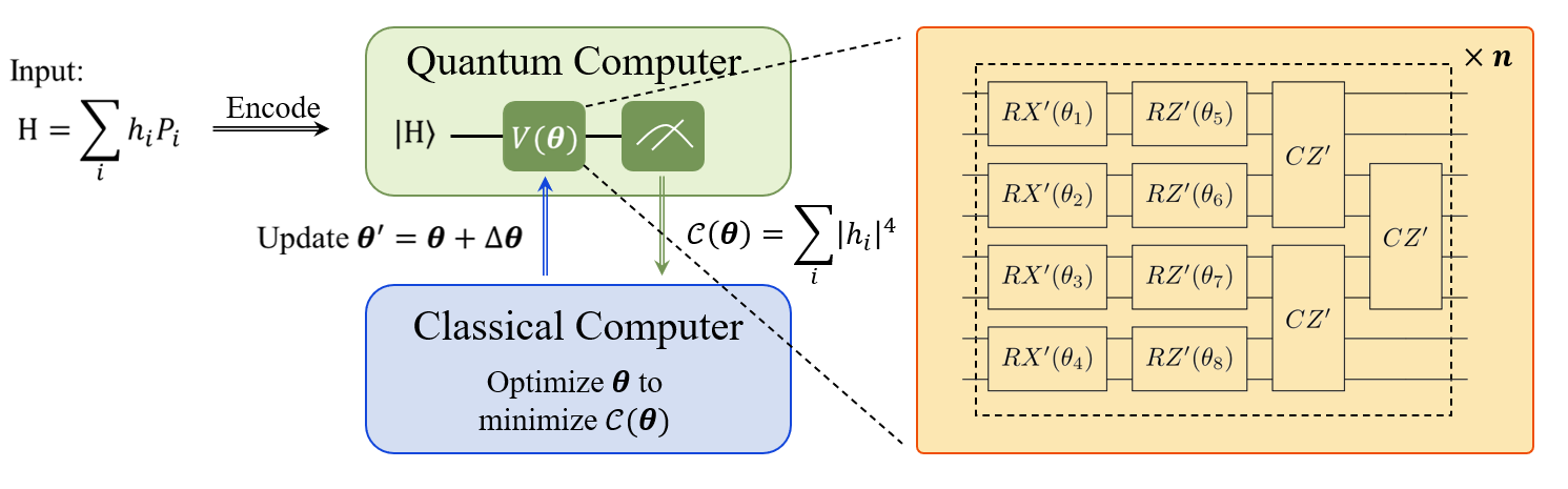
It is well-known that due to the non-convexity of unitary, it is very hard to obtain the optimal unitary to satisfy our requirement as shown in Eq. (14). Here we propose to apply the variational quantum algorithm (VQA) to approach the optimal unitary. The workflow of our algorithm is shown in Fig. 1. At the beginning, we encode the Hamiltonian into a quantum state. Randomize the parameters in the PQC, and estimate the cost function by measurement. Then we use a classical computer to optimize the parameters in the PQC and update the parameters correspondingly. Repeat this process until the cost function is minimized.
In this section, we are going to present the details of the cost function and the choice of PQC in the algorithm design. The specific algorithm is also provided as shown in Algorithm 1.
III.1 Cost function
We have shown that the complexities of many tasks depend on the Pauli norm of the Hamiltonian, such as expectation value estimation Crawford et al. (2021) and Hamiltonian simulation Campbell (2019). We then convert the problem of minimizing the Pauli norm (Eq. (3)) to the problem of minimizing the -norm of Hamiltonian vector (Eq. (14)). It is natural to consider the -norm of the corresponding Hamiltonian state as the cost function, i.e., . However, estimating the -norm of a quantum state is generally hard on quantum devices. Fortunately, there is a quantum algorithm that can efficiently estimate the sum of the fourth power of elements in the Hamilton vector , i.e.,
| (22) |
where is the dimension of the system. The detail of the algorithm to estimate the quantity is shown in the Appendix A. This algorithm is also used in inverse participation ratio estimation Liu et al. (2024). Both -norm and describe the uncertainty of a quantum state. From this point of view, minimizing -norm and maximizing have the same optimizing direction, which reduces the uncertainty of a quantum state. Thus, we set as the cost function, i.e.,
| (23) |
Although minimizing -norm and maximizing is not exactly the same problem, the effectiveness of setting as the cost function emerges in the numerical experiment in Sec. IV.4.
III.2 Parameterized quantum circuit
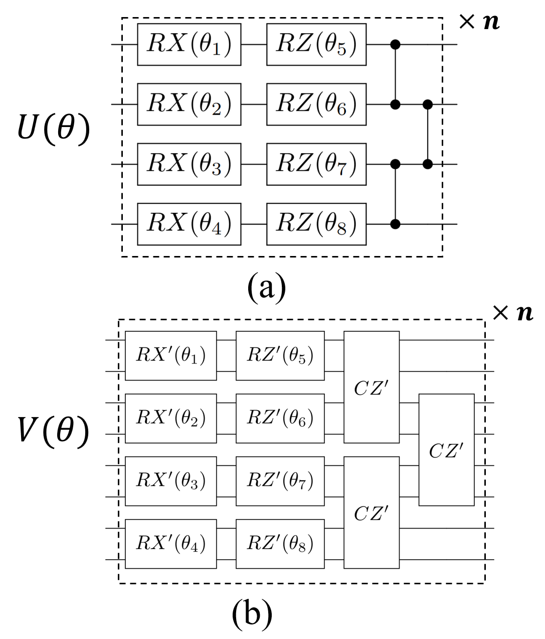
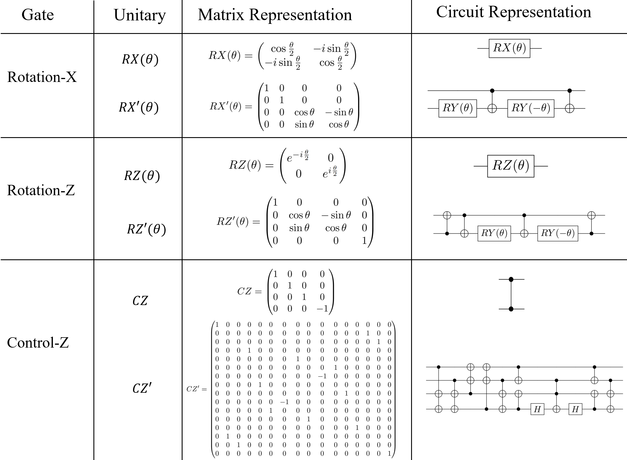
From Theorem 1, the encoded unitary is constructed from the unitary , so and have a one-to-one correspondence relation. We can consider unitary as a function of unitary , i.e., . The function maps an -qubit unitary into a -qubit unitary . Here we take the hardware-efficient ansatz for as shown in Fig. 2 (a), and we automatically obtain the corresponding encoded ansatz as shown in Fig. 2 (b). The ansatz for contains single qubit rotation gates rotation-X (RX), rotation-Z (RZ), and entangled gates control-Z (CZ). The corresponding encoded unitary components are denoted as RX’, RZ’, and CZ’, whose detailed information is shown in Appendix B. The encoded unitaries are all real, thus there is no need to worry about the imaginary element in the optimized Hamiltonian state. There is one thing we need to note that and share the same parameters . Once the parameters optimization in unitary is done, we can obtain the unitary directly by inserting the parameters into . The unitary is necessary when we apply the algorithm to expectation value estimation and Hamiltonian simulation, which will be discussed in Sec. IV.
IV Application
In this section, we are going to apply the proposed algorithm to reduce the measurement time in the task of expectation value estimation and the gate count in the task of Hamiltonian simulation, respectively. We especially emphasize that the proposed VQHE is compatible with grouping, which is another method to reduce the measurement complexity. The measurement complexity can be reduced for a further step. We also propose a partition trick to tackle the issue of scalability.
To apply the engineered Hamiltonian to the tasks of expectation value estimation and Hamiltonian simulation, we must first obtain the engineered Pauli coefficients . Quantum state tomography Nielsen and Chuang (2010) is a candidate to get such information from the engineered Hamiltonian state . However, the cost of state tomography increases exponentially with respect to the system size. Fortunately, the engineered Hamiltonian state is optimized by reducing its uncertainty, hence the complex amplitude is expected to be concentrated on a certain computational basis. In other words, we expect the engineered Hamiltonian state to be a sparse pure state. In Ref. Gulbahar (2021), a more efficient algorithm than quantum state tomography was proposed to reconstruct the sparse pure state. With the engineered Hamiltonian coefficients , the -norm of the engineered Hamiltonian norm can be calculated straightforwardly.
IV.1 Expectation value estimation
In quantum computing, estimating the expectation value of a Hamiltonian to a quantum state, i.e., , is one of the most fundamental processes in many tasks. The total measurement time is determined by the Pauli norm, i.e., . In order to reduce the measurement time, we can apply the proposed VQHE algorithm first as shown in Algorithm 1 as a pre-processing, which returns us the engineered Hamiltonian state and the optimized parameters . Then estimate the engineered Pauli coefficients from the engineered Hamiltonian state . The optimized Hamiltonian norm is obtained by summing up all the absolute values of the coefficients, i.e., .
When we estimate the expectation value of Hamiltonian , we have
| (24) |
where is the engineered Hamiltonian. Here we set the unitary as , where is the Ansatz shown in Fig. 2 (a), and the parameters are optimized by Algorithm 1. In this case, the corresponding measurement time of estimating Hamiltonian reduces to .
The measurement time can be reduced further by applying a grouping algorithm to the engineered Hamiltonian. Grouping Kandala et al. (2017); Gokhale et al. (2019); Verteletskyi et al. (2020); Crawford et al. (2021) is an efficient classical algorithm to reduce the measurement time in the task of expectation value estimation. The main idea of grouping is dividing the Pauli terms into collections, such that all the Pauli elements in a collection commute with each other, thus they can be measured simultaneously. Many grouping methods have been proposed, such as qubit-wise commuting (QWC) Kandala et al. (2017), general commuting (GC) Gokhale et al. (2019); Verteletskyi et al. (2020), and sorted insertion Crawford et al. (2021). Here we focus on the sorted insertion strategy, which is described as follows, and the details of QWC and GC can be found in the Appendix C.
For a given Hamiltonian as shown in Eq. (2), the set is sorted by the absolute value of coefficients so that . Then, in the order , it is checked whether commutes with all elements in an existing collection. If it does, it is added to that collection. If not, a new collection is created and is inserted there. The collections are checked in order of their creation. After division, there are collections in total, and the -th collection has Pauli terms. Here denote the grouped Pauli norm as , which is highly dependent on the group strategy. The total measurement time of the grouped collections is proportional to the square of the which is Crawford et al. (2021). The details and examples are shown in the Appendix D. If we apply the VQHE algorithm followed by the sorted grouping algorithm, the corresponding measurement time will be
| (25) |
IV.2 Hamiltonian simulation with qDrift
Consider a Hamiltonian , where is hermitian and normalized, is the weight. For each , the unitary can be implemented on quantum computers for any . In the Trotter formulae, one divides into segments so that with and uses to approach in the large limit. Repeat this process for times such that in the large limit. It has been proven in Refs. Childs et al. (2019, 2018) that the total gate count is , where is the magnitude of the strongest term in the Hamiltonian, is the error tolerance. The gate count of this method depends on the terms of decomposition, which is not practical for electronic structure Hamiltonians due to its large number of terms.
The quantum stochastic drift protocol (qDrift) Campbell (2019) was proposed to solve this problem. Each unitary in the sequence is chosen independently from an identical distribution. Denote . The strength of each unitary is fixed , which is independent of , so we implement gates of the form . Then we randomly choose the unitary with probability . The full circuit is described by an ordered list of values that corresponds to unitary
| (26) |
which is selected from the product distribution . The gate count of Hamiltonian simulation by qDrift method is , where is the Pauli norm of Hamiltonian.
Before simulating a given Hamiltonian , we can first apply the VQHE algorithm to engineer the Hamiltonian such that the Pauli norm of the engineered Hamiltonian is reduced. Instead of simulating the original Hamiltonian, we can simulate the engineered Hamiltonian. Because of Eq. (27)
| (27) |
we need to sandwich the Hamiltonian evolution by unitaries. The corresponding gate count of simulating the engineered Hamiltonian is
| (28) |
where , and is the gate count of the unitary, which can be ignored because it is a constant. The proof of Eq. (27) is shown in Appendix E.
IV.3 Scalability
One obstacle to variational quantum algorithms is barren plateaus McClean et al. (2018); Marrero et al. (2021); kai Zhang et al. (2023), which refers to the phenomenon that the gradient decreases exponentially with the increase of the quantum system. To solve this problem, we propose a straightforward trick called partition trick. Briefly speaking, we can divide the Hamiltonian into parts, where they have common factors. For each part, we extract the common factors and apply the VQHE to the rest Hamiltonian. We take the Hamiltonian as an example. We can first divide the Hamiltonian into two parts, and extract the common factor, thus we have and . Then we apply VQHE to minimize and , respectively. The engineered Hamiltonian will be with and similarly .
The partition trick is compatible with estimating expectation value. When we estimate the expectation value, we have
| (29) |
where is the partite sub-Hamiltonian, and is the engineered sub-Hamiltonian. We should estimate the expectation values of each sub-Hamiltonian first, then sum them up. In such a case, the measurement time is . In the task of Hamiltonian simulation, Eq. (27) doesn’t hold anymore, for the unitaries are not the same for different partition Hamiltonian . The partition trick is not compatible with Hamiltonian simulation.
The partition trick gets rid of barren plateaus by dividing a big optimization problem into several small ones, which helps us find the effective unitary to reduce the Pauli norm. However, such a trick will also reduce the expressibility of the ansatz, making us unlikely to obtain the optimal unitary to engineer Hamiltonian. This trick can be understood as a trade-off between effectiveness and optimality.
IV.4 Numerical experiments
In this part, we are going to show the effectiveness of the proposed VQHE, which can reduce the Pauli norm of Hamiltonian. Specifically, we apply VQHE to the Ising Hamiltonian and the molecules’ Hamiltonian.
Ising model, a mathematical model of ferromagnetism in statistical mechanics, involves representing a material as a lattice of discrete points, where each point or "spin" can be in one of two possible states, typically denoted as "up" or "down." The spins interact with their nearest neighbors, and the interactions are characterized by a coupling constant. The Hamiltonian of the Ising model describes the energy of the system and is given by the sum of the interactions between neighboring spins. The basic form of the Hamiltonian for a one-dimensional Ising model is where refers to the sit.
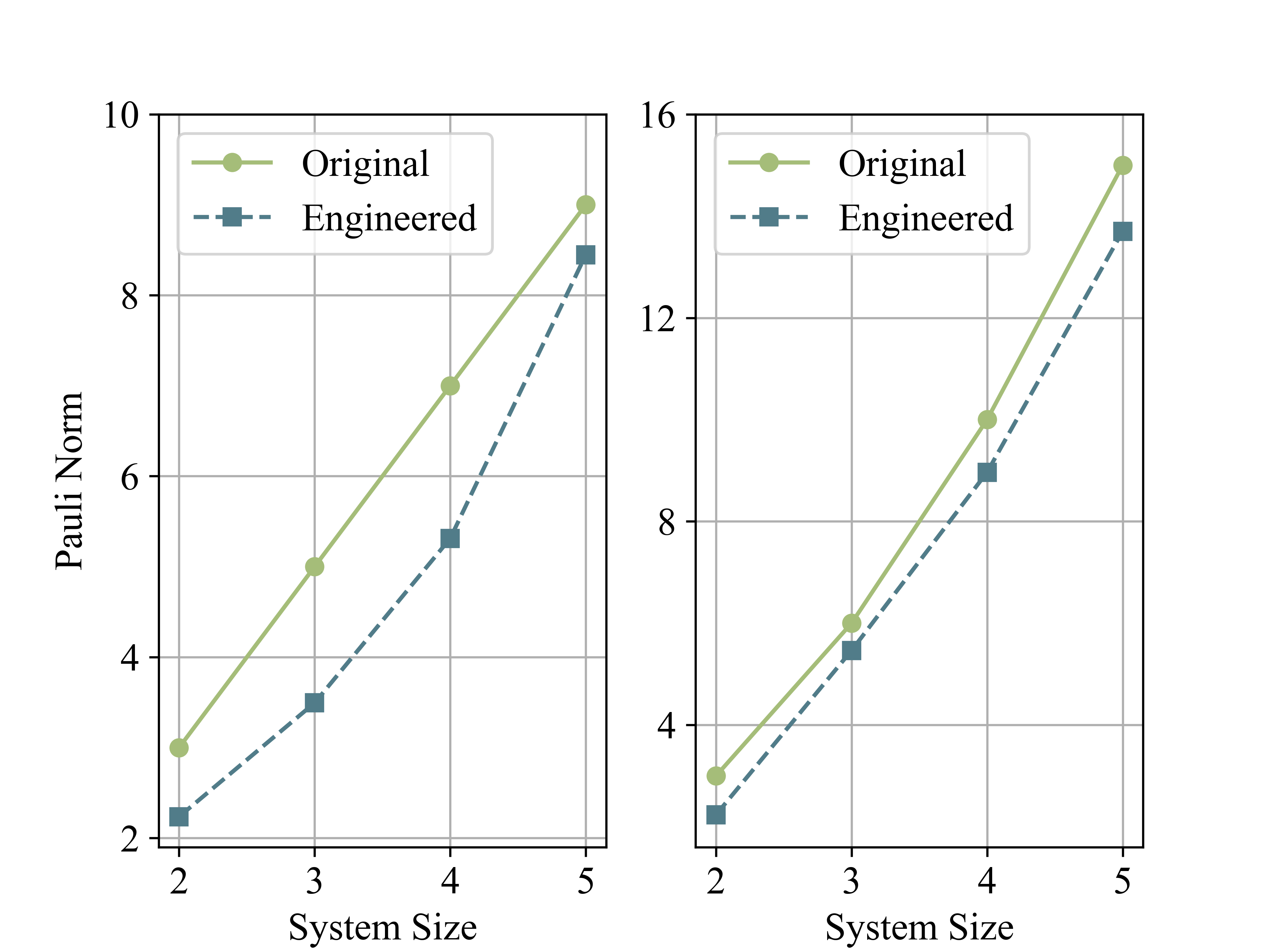
In the first numerical experiment, we apply the VQHE algorithm to the Ising model with different system sizes and compare the original Pauli norm and the engineered Pauli norm. For convenience, we set the coefficients in the Ising Hamiltonian to be the same, i.e., . In this experiment, we consider two Hamiltonians which are neighbor Ising Hamiltonian () and all-to-all Ising Hamiltonian ( and are independent), respectively. Specifically, we have
| (30) | |||
| (31) |
where and refer to Pauli-X and Pauli-Z operators, respectively. From the numerical results (Fig. 3), the engineered Hamiltonian shows advantages over the original Hamiltonian with smaller Pauli norms in both cases of neighbor Ising Hamiltonian and all-to-all Ising Hamiltonian.
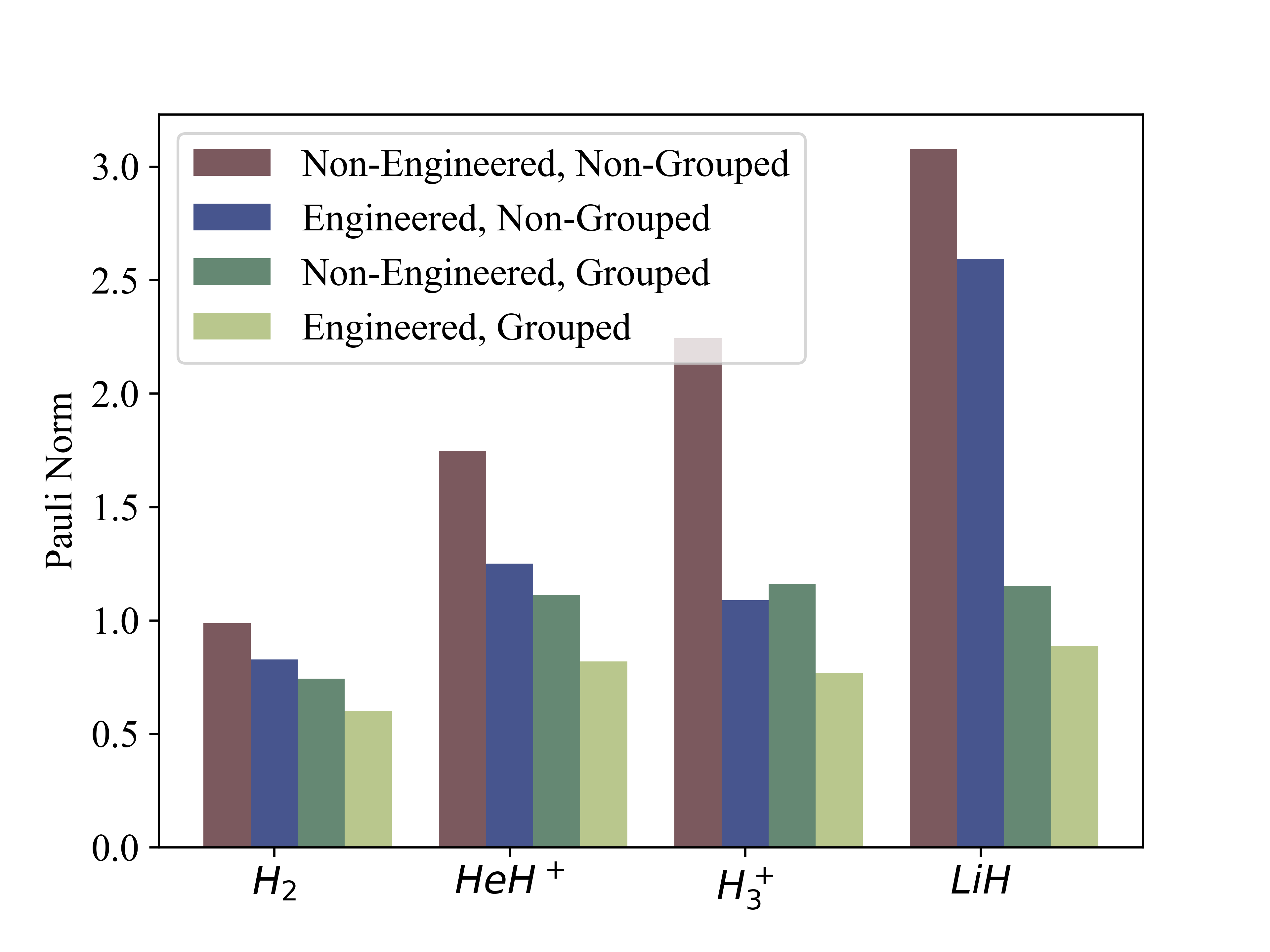
We also conduct numerical experiments on more complicated systems, including , , , and molecules. In this experiment, we apply VQHE to the tapered Hamiltonian Bravyi et al. (2017); Setia et al. (2020) of molecules for simplicity. The qubit tapering approach encodes the original quantum system into a smaller system, which preserves the ground state and ground energy. Thus, the tapered Hamiltonian reduces the requirement of the number of qubits, making the variational quantum eigensolver (VQE) Kandala et al. (2017) more efficient. By applying VQHE to the tapered Hamiltonian of molecules, one observes the engineered Hamiltonian has a smaller Pauli norm compared with the original one. For a further step, we also take the sorted insertion grouping strategy into consideration. Specifically, we engineer the Hamiltonian with VQHE first, then apply the sorted insertion grouping method to the engineered Hamiltonian. The numerical results in Fig. 4 show that the engineered grouped Pauli norm of Hamiltonian can be reduced further compared with that of engineered Hamiltonian and that of grouped Hamiltonian . These results emphasize that the proposed VQHE is compatible with the grouping strategies.
V Conclusion
In this work, we propose the VQHE algorithm to reduce the Pauli norm of Hamiltonian such that the overheads for expectation value and Hamiltonian simulation can be reduced. We first develop the theory to convert the Pauli norm optimization problem into the vector -norm minimization problem, and then design the cost function and parameterized quantum circuits to minimize Pauli norm variationally. We then display how to apply the proposed VQHE algorithm to expectation value estimation and Hamiltonian simulation. In the task of expectation value estimation, we also emphasize that the proposed algorithm is compatible with grouping, such that the measurement time can be reduced further. The numerical experiments are conducted by applying the VQHE algorithms to the Ising Hamiltonian and some molecules’ Hamiltonian, which shows the effectiveness of VQHE algorithm.
For further research, it would also be fun to find the optimized Pauli norm of Hamiltonian we could obtain. It will also be interesting to apply the proposed algorithm VQHE to other applications in quantum computing. Besides, this framework may also be applied to tensor networks, empowering classical computers to solve quantum problems.
Acknowledgments.– B.Z would like to thank Hideaki Hakoshima, Xuanqiang Zhao, and Xin Wang for their fruitful discussion. This work is supported by MEXT Quantum Leap Flagship Program (MEXT Q-LEAP) Grant No. JPMXS0118067394 and JPMXS0120319794, and JST COINEXT Grant No. JPMJPF2014.
References
- Farhi et al. (2014) E. Farhi, J. Goldstone, and S. Gutmann, arXiv preprint arXiv:1411.4028 (2014).
- Harrigan et al. (2021) M. P. Harrigan, K. J. Sung, M. Neeley, K. J. Satzinger, F. Arute, K. Arya, J. Atalaya, J. C. Bardin, R. Barends, S. Boixo, et al., Nature Physics 17, 332 (2021).
- McArdle et al. (2020) S. McArdle, S. Endo, A. Aspuru-Guzik, S. C. Benjamin, and X. Yuan, Reviews of Modern Physics 92, 015003 (2020).
- Quantum et al. (2020) G. A. Quantum, Collaborators*†, F. Arute, K. Arya, R. Babbush, D. Bacon, J. C. Bardin, R. Barends, S. Boixo, M. Broughton, B. B. Buckley, et al., Science 369, 1084 (2020).
- Bennett and Brassard (2014) C. H. Bennett and G. Brassard, Theoretical computer science 560, 7 (2014).
- Ekert (1991) A. K. Ekert, Physical review letters 67, 661 (1991).
- Biamonte et al. (2017) J. Biamonte, P. Wittek, N. Pancotti, P. Rebentrost, N. Wiebe, and S. Lloyd, Nature 549, 195 (2017).
- Kandala et al. (2017) A. Kandala, A. Mezzacapo, K. Temme, M. Takita, M. Brink, J. M. Chow, and J. M. Gambetta, Nature 549, 242 (2017).
- McClean et al. (2016) J. R. McClean, J. Romero, R. Babbush, and A. Aspuru-Guzik, New Journal of Physics 18, 023023 (2016).
- Wecker et al. (2015) D. Wecker, M. B. Hastings, and M. Troyer, Physical Review A 92, 042303 (2015).
- Huggins et al. (2021) W. J. Huggins, J. R. McClean, N. C. Rubin, Z. Jiang, N. Wiebe, K. B. Whaley, and R. Babbush, npj Quantum Information 7, 1 (2021).
- Rubin et al. (2018) N. C. Rubin, R. Babbush, and J. McClean, New Journal of Physics 20, 053020 (2018).
- Trotter (1959) H. F. Trotter, Proceedings of the American Mathematical Society 10, 545 (1959).
- Suzuki (1991) M. Suzuki, Journal of Mathematical Physics 32, 400 (1991).
- Campbell (2019) E. Campbell, Physical review letters 123, 070503 (2019).
- Cerezo et al. (2021) M. Cerezo, A. Arrasmith, R. Babbush, S. C. Benjamin, S. Endo, K. Fujii, J. R. McClean, K. Mitarai, X. Yuan, L. Cincio, et al., Nature Reviews Physics 3, 625 (2021).
- Mitarai et al. (2018) K. Mitarai, M. Negoro, M. Kitagawa, and K. Fujii, Physical Review A 98, 032309 (2018).
- Benedetti et al. (2019) M. Benedetti, E. Lloyd, S. Sack, and M. Fiorentini, Quantum Science and Technology 4, 043001 (2019).
- Peruzzo et al. (2014) A. Peruzzo, J. McClean, P. Shadbolt, M.-H. Yung, X.-Q. Zhou, P. J. Love, A. Aspuru-Guzik, and J. L. O’brien, Nature communications 5, 4213 (2014).
- McClean et al. (2017) J. R. McClean, M. E. Kimchi-Schwartz, J. Carter, and W. A. De Jong, Physical Review A 95, 042308 (2017).
- Nakanishi et al. (2019) K. M. Nakanishi, K. Mitarai, and K. Fujii, Physical Review Research 1, 033062 (2019).
- Schuld et al. (2020) M. Schuld, A. Bocharov, K. M. Svore, and N. Wiebe, Physical Review A 101, 032308 (2020).
- Farhi and Neven (2018) E. Farhi and H. Neven, arXiv preprint arXiv:1802.06002 (2018).
- Chen et al. (2023) R. Chen, B. Zhao, and X. Wang, Physical Review Applied 20, 024071 (2023).
- Chen et al. (2021) R. Chen, Z. Song, X. Zhao, and X. Wang, Quantum Science and Technology 7, 015019 (2021).
- Zhao et al. (2021) X. Zhao, B. Zhao, Z. Wang, Z. Song, and X. Wang, npj Quantum Information 7, 159 (2021).
- Romero et al. (2017) J. Romero, J. P. Olson, and A. Aspuru-Guzik, Quantum Science and Technology 2, 045001 (2017).
- Cao and Wang (2021) C. Cao and X. Wang, Physical Review Applied 15, 054012 (2021).
- Wang et al. (2021a) X. Wang, Z. Song, and Y. Wang, Quantum 5, 483 (2021a).
- Zeng et al. (2021) J. Zeng, C. Cao, C. Zhang, P. Xu, and B. Zeng, Quantum Science and Technology 6, 045009 (2021).
- Wang et al. (2021b) Y. Wang, G. Li, and X. Wang, Physical Review Applied 16, 054035 (2021b).
- Crawford et al. (2021) O. Crawford, B. van Straaten, D. Wang, T. Parks, E. Campbell, and S. Brierley, Quantum 5, 385 (2021).
- Gokhale et al. (2019) P. Gokhale, O. Angiuli, Y. Ding, K. Gui, T. Tomesh, M. Suchara, M. Martonosi, and F. T. Chong, arXiv preprint arXiv:1907.13623 (2019).
- Verteletskyi et al. (2020) V. Verteletskyi, T.-C. Yen, and A. F. Izmaylov, The Journal of chemical physics 152, 124114 (2020).
- Zhang et al. (2022) X.-M. Zhang, T. Li, and X. Yuan, Physical Review Letters 129, 230504 (2022).
- Liu et al. (2024) Y. Liu, P. Sierant, P. Stornati, M. Lewenstein, and M. Płodzień, arXiv preprint arXiv:2405.03338 (2024).
- Nielsen and Chuang (2010) M. A. Nielsen and I. L. Chuang, Quantum computation and quantum information (Cambridge university press, 2010).
- Gulbahar (2021) B. Gulbahar, arXiv preprint arXiv:2111.04359 (2021).
- Childs et al. (2019) A. M. Childs, A. Ostrander, and Y. Su, Quantum 3, 182 (2019).
- Childs et al. (2018) A. M. Childs, D. Maslov, Y. Nam, N. J. Ross, and Y. Su, Proceedings of the National Academy of Sciences 115, 9456 (2018).
- McClean et al. (2018) J. R. McClean, S. Boixo, V. N. Smelyanskiy, R. Babbush, and H. Neven, Nature communications 9, 4812 (2018).
- Marrero et al. (2021) C. O. Marrero, M. Kieferová, and N. Wiebe, PRX Quantum 2, 040316 (2021).
- kai Zhang et al. (2023) H. kai Zhang, C. Zhu, M. Jing, and X. Wang, “Statistical analysis of quantum state learning process in quantum neural networks,” (2023), arXiv:2309.14980 [quant-ph] .
- Bravyi et al. (2017) S. Bravyi, J. M. Gambetta, A. Mezzacapo, and K. Temme, arXiv preprint arXiv:1701.08213 (2017).
- Setia et al. (2020) K. Setia, R. Chen, J. E. Rice, A. Mezzacapo, M. Pistoia, and J. D. Whitfield, Journal of Chemical Theory and Computation 16, 6091 (2020).
- Aguado et al. (2021) A. Aguado, O. Roncero, and C. Sanz-Sanz, Physical Chemistry Chemical Physics 23, 7735 (2021).
- Yen et al. (2020) T.-C. Yen, V. Verteletskyi, and A. F. Izmaylov, Journal of chemical theory and computation 16, 2400 (2020).
- Romero et al. (2018) J. Romero, R. Babbush, J. R. McClean, C. Hempel, P. J. Love, and A. Aspuru-Guzik, Quantum Science and Technology 4, 014008 (2018).
Supplementary Material for
variational quantum Hamiltonian engineering
Appendix A Quantum algorithm for estimating
We denote the summation of the fourth power of elements in an -qubit pure state as , which is
| (32) |
where refers to the computational basis. There exists an efficient quantum algorithm to estimate the quantity , which is shown in Fig. 5.
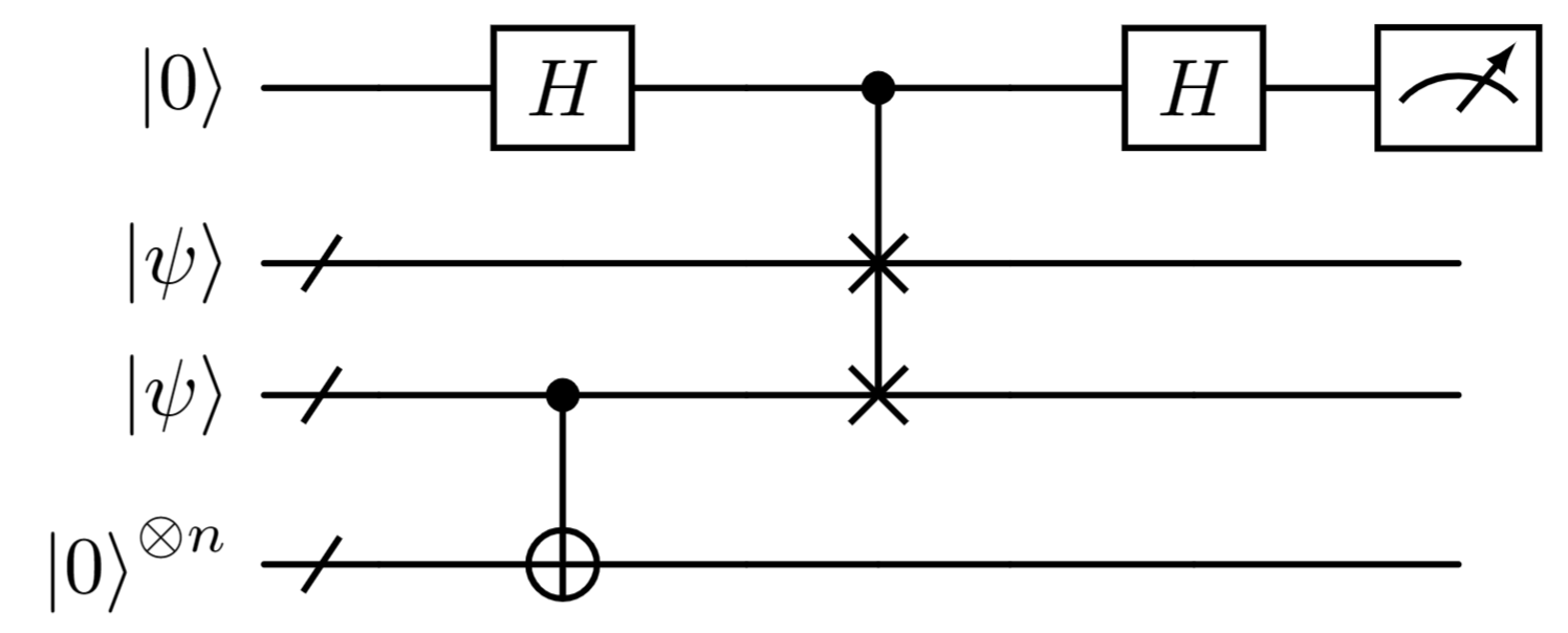
The first step of the algorithm is to initialize the quantum state. We need four registers in total. The first register is called the measurement register, which is initialized as . The second and third registers are prepared as the -qubit quantum state . The last register is prepared as -qubit zero state . At the beginning, we have
| (33) |
Apply CNOT gates on the third and fourth register, we then have
| (34) |
At this step, we can discard the fourth register and the quantum state on the third register becomes a mixed state . Take the SWAP test on the first three registers, the probability of getting the measurement as +1 is
| (35) |
where is the desired value.
In Ref. Liu et al. (2024), A similar algorithm is also used in inverse participation ratio estimation.
Appendix B Gate correspondence
Appendix C Measurement time of grouping
In a normal distribution approximation, we require a variance of in the estimator . Then, the ground energy can be measured,
| (36) |
However, this straightforward method requires a huge amount of measurement time, making it infeasible to estimate the ground energy in large system. The standard error on the mean energy after taking samples for each Pauli operator is
| (37) |
If the measurement time of each term are the same Kandala et al. (2017); McClean et al. (2016), then the total measurement time is
| (38) |
where is the maximum coefficient.
If we choose , and bounding the variances by Var, then we get Wecker et al. (2015); Huggins et al. (2021); Rubin et al. (2018)
| (39) |
This inequality was proved in Rubin et al. (2018). If we insist on getting an asymptotic bound then we assume Var, then the measurement time is optimal as in Eq. (39)
After measurements, we get a set of values which is composed of 0 and 1, then the estimated expected value and its variance
| (40) | ||||
| (41) |
Clearly, when the system becomes complicated, it is hard to make measurement for the huge amount of resource requirements. From Eq. (38), the fewer terms of the Hamiltonian, the less measurement time will be. Since commuting Pauli terms can be measured simultaneously, one straightforward idea is to partition the Pauli terms into groups, and in each group, all elements commute with each other. This kind of method is called Clique Cover. If the number of such groups is minimum, it is called Minimum Clique Cover.
C.1 Qubit wise commuting (QWC)
Qubit-wise commuting (QWC)Kandala et al. (2017) is one of the simplest methods to partition the Hamiltonian terms, which only group the terms that commute in qubit wise. For example is a QWC group because commutes with and commutes with . While the case of is not a QWC group for and do not commute. When doing the measurement, we only need to apply for local Clifford unitary . This method can decrease 70% terms.
C.2 General commuting (GC)
The general commuting method Gokhale et al. (2019); Verteletskyi et al. (2020) is a more powerful method compared with QWC. Note that QWC is simply the subset of GC corresponding to the case where the number of non-commuting indices is 0. When we make measurements, we need to apply the unitary transfer to the GC group into QWC group such that we can make measurements directly, i.e.,
| (42) | ||||
| (43) | ||||
| (44) | ||||
| (45) |
where is the corresponding QWC group. The unitary can be decomposed into Clifford gates. This method can decrease two two-magnitude number of terms.
After partitioning into GC groups, we need to apply unitaries first, and then make simultaneous measurements. Since the unitaries are Clifford Yen et al. (2020), the coefficient won’t change after the unitary, therefore the
Appendix D The Grouped Pauli Norm
For a given operator , we have
| (46) |
where is the number of collections of mutually commuting operators, the number of operators in collection , is the Pauli operator in the th collection and is its coefficient.
It has been proved Romero et al. (2018); Wecker et al. (2015); Rubin et al. (2018) that the optimal number of measurements of collection is
| (47) |
Therefore, the total number of measurements is
| (48) |
where
| (49) |
Theorem 3
Gokhale et al. (2019) Given , two commuting but non-identical Pauli strings, where the expectation is taken over a uniform distribution over all possible state vectors.
For convenience, we assume we do not know the quantum state, and replace the variances and covariances by their expectation value over uniform spherical distribution. From Theorem 3, it is straightforward to have
| (50) |
To make a comparison with the ungrouped Pauli norm of Hamiltonian, we denote it as the grouped Pauli norm
| (51) |
Here we give a simple example by setting the Hamiltonian as . The first step is to sort it by the absolute value of coefficients, which will be . At this stage, no collection is created, so we need to create one for the first element, such that . For the second element , we have to create another collection for anti-commutes to . Now the collections will be . For the third element , it does not commute with the element in the first collection, thus we need to check the commutativity of the second collection. Luckily, the third element commutes with all elements in the second collection, thus we can put it into this collection, which becomes . In this case, the corresponding grouped Pauli norm is , while the Pauli norm without grouping is .
Appendix E Proof of Eq. (27)
When we simulate the engineered Hamiltonian, we have to sandwich it with unitaries, to guarantee that the simulated Hamiltonian is the desired one,
| (52) | ||||
| (53) | ||||
| (54) | ||||
| (55) | ||||
| (56) | ||||
| (57) |
The second and last equations come from the Taylor expansion.