Bilevel Optimization of the Kantorovich Problem and its Quadratic Regularization
Part III: The Finite-Dimensional Case

Abstract.

As the title suggests, this is the third paper in a series addressing bilevel optimization problems that are governed by the Kantorovich problem of optimal transport. These tasks can be reformulated as mathematical problems with complementarity constraints in the space of regular Borel measures. Due to the nonsmoothness that is introduced by the complementarity constraints, such problems are often regularized, for instance, using entropic regularization. In this series of papers, however, we apply a quadratic regularization to the Kantorovich problem. By doing so, we enhance its numerical properties while preserving the sparsity structure of the optimal transportation plan as much as possible. While the first two papers in this series focus on the well-posedness of the regularized bilevel problems and the approximation of solutions to the bilevel optimization problem in the infinite-dimensional case, in this paper, we reproduce these results for the finite-dimensional case and present findings that go well beyond the ones of the previous papers and pave the way for the numerical treatment of the bilevel problems.

1. Introduction

The Kantorovich problem (of optimal transport) is given by

$$\begin{array}[]{rl}\inf\limits_{\pi}&\displaystyle\int_{\Omega_{1}\times\Omega_{2}}c\,\mathop{{\mathrm{d}\pi}}\\[10.00002pt] \text{s.t.}&\pi\in\Pi(\mu_{1},\mu_{2}),\quad\pi\geq 0.\end{array}$$ (K)

In the above, $\Omega_{1}\subset\mathbb{R}^{d_{1}}$ and $\Omega_{2}\subset\mathbb{R}^{d_{2}}$ are (locally) compact domains, $c\colon\Omega_{1}\times\Omega_{2}\to\mathbb{R}$ is a (lower semi-)continuous cost function that is bounded from below, and

$$\Pi(\mu_{1},\mu_{2})\coloneqq\{\pi\in\mathfrak{M}(\Omega_{1}\times\Omega_{2})\colon{P_{1}}_{\#}\pi=\mu_{1},~{}{P_{2}}_{\#}\pi=\mu_{2}\}$$

denotes the set of transport plans between the source marginal $\mu_{1}\in\mathfrak{M}(\Omega_{1})$ and the target marginal $\mu_{2}\in\mathfrak{M}(\Omega_{2})$. Already Kantorovich himself knew that this problem is well-posed, see [16]. In the first two parts of this series of papers, [13, 14], we treated the Kantorovich problem as the lower-level problem of a general bilevel optimization problem, i.e., we investigated problems of the form

$$\begin{array}[]{rl}\inf\limits_{\pi,\mu_{1}}&\mathcal{J}(\pi,\mu_{1})\\[5.0pt] \text{s.t.}&\pi\in\mathfrak{M}(\Omega_{1}\times\Omega_{2}),\quad\mu_{1}\in\mathfrak{M}(\Omega_{1}),\\[5.0pt] &\mu_{1}\geq 0,\quad\|\mu_{1}\|_{\mathfrak{M}(\Omega_{1})}=\|\mu_{2}^{\mathrm{d}}\|_{\mathfrak{M}(\Omega_{2})},\\[5.0pt] &\pi~{}\text{solves (\hyperref@@ii[pr:INTRO-Kant]{K}) w.r.t.}~{}\mu_{1},~{}\mu_{2}^{\mathrm{d}},~{}\text{and}~{}c_{\mathrm{d}},\end{array}$$ (BK)

where $\mathcal{J}\colon\mathfrak{M}(\Omega)\times\mathfrak{M}(\Omega_{1})\to\mathbb{R}\cup\{+\infty\}$ is an arbitrary weak^∗ lower semicontinuous objective functional and $\mu_{2}^{\mathrm{d}}\in\mathfrak{M}(\Omega_{2})$ and $c_{\mathrm{d}}\in C(\Omega_{1}\times\Omega_{2})$ are given (and fixed) data. Depending on the choice of $\mathcal{J}$, (BK) is suited to model different tasks. For instance, if we consider a tracking-type objective of the form

$$\mathcal{J}(\pi,\mu_{1})=\|\pi-\pi_{\mathrm{d}}\|_{\mathfrak{M}(D)}+\|\mu_{1}-\mu_{1}^{\mathrm{d}}\|_{\mathfrak{M}(D_{1})},$$

where $D\subset\Omega_{1}\times\Omega_{2}$ and $D_{1}\subset\Omega_{1}$ are (open) observation domains and $\pi_{\mathrm{d}}\in\mathfrak{M}(D)$ and $\mu_{1}^{\mathrm{d}}\in\mathfrak{M}(D_{1})$ are given data, then the bilevel problem (BK) turns into the task of recovering an (unknown) transportation process from (incomplete and/or noisy) observations of the transport plan and the source marginal. This is a special case of an inverse problem that is governed by the Kantorovich problem. While recovering certain properties of a transportation process from observations is not a new challenge, as a reference we only mention [23, 6, 1] and the references therein, to the author’s best knowledge the above approach is unique as it involves the solution of a single optimization problem, whereas all of the mentioned approaches rely on Bayesian methods.

Another possible application of the general bilevel problem (BK) is given if one considers the compact domains $\Omega_{1}=\Omega_{2}\eqqcolon\Omega_{*}\subset\mathbb{R}^{d_{*}}$, the prior $\mu_{2}^{\mathrm{d}}\in\mathfrak{P}(\Omega_{*})$, the cost $c_{\mathrm{d}}(x,y)=\|x-y\|^{\rho}$, $\rho>1$, and the objective functional

$$\mathcal{J}(\pi,\mu_{1})=\frac{1}{2}\|G\mu_{1}-y_{\mathrm{d}}\|_{Y}+\nu\left(\int_{\Omega_{*}\times\Omega_{*}}c_{\mathrm{d}}\,\mathop{{\mathrm{d}\pi}}\right)^{\frac{1}{\rho}},$$

where $G$ is a compact linear operator mapping the measure space $\mathfrak{M}(\Omega_{*})$ onto some Banach space $Y$, $\nu>0$ is a weighting parameter, and $y_{\mathrm{d}}\in Y$ is a given observation. In this setting, (BK) turns out to be equivalent to the Wasserstein(-regularized) inverse problem

$$\begin{array}[]{rl}\inf\limits_{\mu_{1}}&\frac{1}{2}\|G\mu_{1}-y_{\mathrm{d}}\|_{Y}+\nu W_{\rho}(\mu_{1},\mu_{2}^{\mathrm{d}})^{\rho}\\[5.0pt] \text{s.t.}&\mu_{1}\in\mathfrak{P}(\Omega_{*}),\end{array}$$ (WI_ρ)

which is a linear inverse problem on a probability space with a weighted regularization term added to its target functional. Again, linear inverse problems on measure spaces have been extensively studied in the past, see e.g. [3, 4, 5, 9, 20], just to mention a few. Still, the above optimization is to the author’s best knowledge unique, as it considers a regularization w.r.t. the Wasserstein distance instead of the radon norm. We expect this regularization to be advantageous, because the Wasserstein distance metrizes the weak convergence of probability measures (on Polish spaces), see e.g. [24, Chapter 6].

In [13, 14], we took advantage of a quadratic ($L^{2}$) regularization to improve the properties of the Kantorovich problem (K) and, by replacing the lower-level Kantorovich problem by its $L^{2}$ regularized counterpart and by interposing a smoothing of the involved variables, also the properties of the general bilevel problem (BK). We have shown that both the non-regularized and the regularized bilevel problems are well-posed and that, under some mild regularity conditions on the domains and the given data, by driving the regularization and smoothing parameters to zero, we can approximate certain solutions to the general bilevel problem by means of solutions to the regularized bilevel problems.

In the same spirit, the present paper deals with a discretized version of the Kantorovich problem, which is also known as the Hitchcock problem (of optimal transport). Similar to the infinite-dimensional case of the Kantorovich problem, we introduce a quadratic regularization to improve the numerical properties of both the Hitchcock problem and the corresponding general bi-level problem. However, in contrast to the Kantorovich problem and owing to the finite-dimensional character of the Hitchcock problem, there is no additional smoothing of the variables involved. We replicate the results of the previous papers and in particular improve the results concerning the existence of recovery sequences (which ensure the upper-bound condition in the framework of $\Gamma$-convergence). Furthermore, we introduce an additional regularization of the dual problem of the regularized Hitchcock problem, which allows us to compute (sub)derivatives of the regularized marginal-to-transport plan mapping. In the case that the bilevel objective functional is sufficiently smooth, this then allows us to employ a non-smooth optimization algorithm to (approximately) solve the bilevel problem. In some sense, the present paper is meant to be the basis for the numerical treatment of (discretized) bilevel Kantorovich problems such as the transport identification problem or the Wasserstein inverse problem (WI_ρ) from above.

The present paper is structured as follows: In Section 2, we derive so-called Hitchcock problem as a special case from the infinite-dimensional Kantorovich problem and address the existence of solutions to both itself as well as the corresponding general bilevel problem. We then introduce a quadratic regularization to the Hitchcock problem’s target function, which we then use to regularize the bilevel problem. Furthermore, we show that (in the presence of a recovery sequence), for a vanishing regularization parameter, any cluster point of the sequence of regularized bilevel solutions is a solution to the general bilevel problem. We then present sufficient conditions for the existence of recovery sequences conclude the section with an explicit construction of such a sequence. Section 3 introduces a further quadratic regularization of the dual problem of the regularized Hitchcock problem. Thereby, we can define a regularized marginal-to-transport-plan mapping whose differentiability properties we investigate in detail and which forms the basis of the numerical treatment of the regularized bilevel problems. Finally in Section 4, we present the results of some first numerical tests to verify our findings from the previous sections.

As a disclaimer, most of the results of the present paper can be found, reasonably more detailed, in [12, Part II]. The present work nevertheless provides added value in that we shorten some of the arguments and provide a different perspective on some of the results.

2. The Discrete Kantorovich Problem aka Hitchcock’s Problem

Given $n_{1},n_{2}\in\mathbb{N}$, we consider the finite sets $\Omega_{1}=\{1,\dots,n_{1}\}$ and $\Omega_{2}=\{1,\dots,n_{2}\}$, which we both endow with the discrete topology. We abbreviate their Cartesian product by $\Omega\coloneqq\Omega_{1}\times\Omega_{2}$. Carrying the discrete topology, the Borel sigma algebras $\mathfrak{B}(\Omega_{1})$, $\mathfrak{B}(\Omega_{2})$, and $\mathfrak{B}(\Omega)$ are simply the power sets $\mathcal{P}(\Omega_{1})$, $\mathcal{P}(\Omega_{2})$, and $\mathcal{P}(\Omega)$, respectively.

In the above setting, $\mathfrak{M}(\Omega_{1})\cong\mathbb{R}^{n_{1}}$ and $\mathfrak{M}(\Omega_{2})\cong\mathbb{R}^{n_{2}}$ as well as $\mathfrak{M}(\Omega),C(\Omega)\cong\mathbb{R}^{n_{1}\times n_{2}}$. Consequently, any regular Borel measure $\mu_{i}\in\mathfrak{M}(\Omega_{i})$, $i=1,2$, can be represented by some vector $\vec{\mu}_{i}\in\mathbb{R}^{n_{i}}$ that satisfies $\|\mu_{i}\|_{\mathfrak{M}(\Omega_{i})}=\|\vec{\mu}_{i}\|_{1}$. Of course, the same holds the elements of $\mathfrak{M}(\Omega)$ and $C(\Omega)$, i.e., for every measure $\mu\in\mathfrak{M}(\Omega)$ and every function in $f\in C(\Omega)$, we can always find matrix representations $M,F\in\mathbb{R}^{n_{1}\times n_{2}}$ such that $\|\mu\|_{\mathfrak{M}(\Omega)}=\|M\|_{1}$ and $\|f\|_{C(\Omega)}=\|F\|_{\infty}$. To ease the notation, in the following we will use the same symbol for elements of the measure spaces/function spaces and their representing vectors and matrices.

With this convention, we find that the Kantorovich problem (K) from Section 1 is equivalent to the problem

$$\begin{array}[]{rl}\inf\limits_{\pi}&\langle c,\,\pi\rangle_{F}\\[5.0pt] \text{s.t.}&\pi\in\mathbb{R}^{n_{1}\times n_{2}},\quad\pi\geq 0,\\[5.0pt] &\pi\Mathbb{1}=\mu_{1},\quad\pi^{\top}\Mathbb{1}=\mu_{2},\end{array}$$ (H)

which is known as the Hitchcock problem (of optimal transportation) and finds widespread application throughout different fields of mathematics and economics, see e.g. [11] and the references therein. In the above and the rest of this paper, the symbol $\Mathbb{1}$ refers to the vector (of any dimension) that consists only of ones, i.e., $\Mathbb{1}=(1,\dots,1)^{\top}$. Moreover, $\langle\boldsymbol{\cdot},\,\boldsymbol{\cdot}\rangle_{F}$ denotes the Frobenius scalar product.

The Hitchcock problem is the problem of minimizing a continuous target function over a compact feasible set. We therefore immediately receive the following result:

Theorem 2.1.

For any pair of compatible marginals $\mu_{1}\in\mathbb{R}^{n_{1}}$ and $\mu_{2}\in\mathbb{R}^{n_{2}}$ with $\mu_{1},\mu_{2}\geq 0$ and $\mu_{1}^{\top}\Mathbb{1}=\mu_{2}^{\top}\Mathbb{1}$ as well as for any cost matrix $c\in\mathbb{R}^{n_{1}\times n_{2}}$, the Hitchcock problem (H) has at least one optimal solution.

Analogously to the case of the infinite-dimensional bilevel Kantorovich problem which we introduced in Section 1 and discussed in detail in [13, 14], in this paper we are interested in a bilevel problem that is governed by the finite-dimensional Hitchcock problem.

Let $\mathcal{J}\colon\mathbb{R}^{n_{1}\times n_{2}}\times\mathbb{R}^{n_{1}}\to\mathbb{R}\cup\{+\infty\}$ be some given lower semicontinuous objective function that is bounded on bounded sets, i.e., for all $M>0$ it holds that

$$\sup_{\|(\pi,\mu_{1})\|<M}\mathcal{J}(\pi,\mu_{1})<\infty.$$

Furthermore, consider some fixed target marginal $\mu_{2}^{\mathrm{d}}\in\mathbb{R}^{n_{2}}$ and some fixed cost matrix $c_{\mathrm{d}}\in\mathbb{R}^{n_{1}\times n_{2}}$. For the entirety of this paper, we are interested in the bilevel Hitchcock problem that is given by

$$\begin{array}[]{rl}\displaystyle\inf_{\pi,\mu_{1}}&\mathcal{J}(\pi,\mu_{1})\\[5.0pt] \text{s.t.}&\pi\in\mathbb{R}^{n_{1}\times n_{2}},\quad\mu_{1}\in\mathbb{R}^{n_{1}},\\[5.0pt] &\mu_{1}\geq 0,\quad\mu_{1}^{\top}\Mathbb{1}={\mu_{2}^{\mathrm{d}}}^{\top}\Mathbb{1},\\[5.0pt] &\pi~{}\text{solves \eqref{pr:PROB-Hitch} w.r.t.}~{}\mu_{1},~{}\mu_{2}^{\mathrm{d}},~{}\text{and}~{}c_{\mathrm{d}}.\end{array}$$ (BH)

The bilevel Hitchcock problem (BH) can be seen as a discretization of the bilevel Kantorovich problem (BK). It will therefore form the basis for the numerical treatment of problems such as the transportation identification problem as well as the Wasserstein inverse problem (WI_ρ) which we briefly motivated in Section 1 and were already thoroughly discussed in [14, Section 4].

To show that the bilevel Hitchcock problem (BH) has an optimal solution, we first prove the following lemma that is a finite-dimensional analog of [14, Lemma 3.2] but comes with a shorter proof.

Lemma 2.2.

Let $\mu_{1}\in\mathbb{R}^{n_{1}}$ and $\mu_{2}\in\mathbb{R}^{n_{2}}$ with $\mu_{1},\mu_{2}\geq 0$ and $\mu_{1}^{\top}\Mathbb{1}=\mu_{2}^{\top}\Mathbb{1}$ be given. Consider a sequence of nonnegative marginals $(\mu_{1,k})_{k\in\mathbb{N}}\subset\mathbb{R}^{n_{1}}$ with $\mu_{1,k}^{\top}\Mathbb{1}=\mu_{2}^{\top}\Mathbb{1}$ for all $k\in\mathbb{N}$ and $\mu_{1,k}\to\mu_{1}$ as $k\to\infty$. Then, for any $\pi\in\Pi(\mu_{1},\mu_{2})$, there exists a sequence of nonnegative couplings $(\pi_{k})_{k\in\mathbb{N}}$ with $\pi_{k}\in\Pi(\mu_{1,k},\mu_{2})$ for all $k\in\mathbb{N}$ and $\pi_{k}\to\pi$ as $k\to\infty$.

Proof.

For any $k\in\mathbb{N}$, there exists a nonnegative optimal coupling $\theta_{k}\in\Pi(\mu_{1,k},\mu_{2})$ w.r.t. the metric cost $c(i,j)=|i-j|$ which we use to define the coupling

$$\pi_{k}^{i_{1},i_{2}}\coloneqq\sum_{l\in\Omega_{1}}\frac{\theta_{k}^{i_{1},l}\pi_{l,i_{2}}}{\mu_{1}^{l}}\quad\text{for all}~{}(i_{1},i_{2})\in\Omega.$$

By construction, $\pi_{k}$ is nonnegative and $\pi_{k}\in\Pi(\mu_{1,k},\mu_{2})$. It therefore remains to show the convergence $\pi_{k}\to\pi$.

Using Santambrogio’s stability theorem [21, Theorem 1.50], one easily verifies that the sequence $(\theta_{k})_{k\in\mathbb{N}}$ converges to $\bar{\theta}=\operatorname{diag}(\mu_{1})\in\Pi(\mu_{1},\mu_{1})$, which is the unique optimal coupling transporting $\mu_{1}$ onto itself w.r.t. to $c$. Consequently, for all $(i_{1},i_{2})\in\Omega$,

$$\pi_{k}^{i_{1},i_{2}}=\sum_{l\in\Omega_{1}}\frac{\theta_{k}^{i_{1},l}\pi_{l,i_{2}}}{\mu_{1}^{l}}~{}\xrightarrow[k\to\infty]{}~{}\sum_{l\in\Omega_{1}}\frac{\bar{\theta}_{i_{1},l}\pi_{l,i_{2}}}{\mu_{1}^{l}}=\frac{\bar{\theta}_{i_{1},i_{1}}\pi_{i_{1},i_{2}}}{\mu_{1}^{i_{1}}}=\pi_{i_{1},i_{2}},$$

which proves the claim. ∎

With the above lemma, we can show that the feasible set of the bilevel Hitchcock problem is again compact.

Lemma 2.3.

For any $\mu_{2}\in\mathbb{R}^{n_{2}}$ and any $c\in\mathbb{R}^{n_{1}\times n_{2}}$, the set

$$\mathcal{F}\coloneqq\bigl{\{}(\pi,\mu_{1})\colon\mu_{1}\geq 0,~{}\mu_{1}^{\top}\Mathbb{1}=\mu_{2}^{\top}\Mathbb{1},~{}\pi\,\text{solves \eqref{pr:PROB-Hitch} w.r.t.}\,\mu_{1},\,\mu_{2},\,c\bigr{\}}$$

is non-empty and compact.

Proof.

The non-emptiness of $\mathcal{F}$ is guaranteed by Theorem 2.1. Its boundedness follows from the linear constraints of (H). To see that it is also closed, let us consider a sequence $(\pi_{k},\mu_{1,k})_{k\in\mathbb{N}}\subset\mathcal{F}$ with $(\pi_{k},\mu_{1,k})\to(\pi,\mu_{1})$ as $k\to\infty$. That the limit $\pi$ is feasible for (H) w.r.t. $\mu_{1}$ and $\mu_{2}$ again follows from the linear constraints of the Hitchcock problem. To show that it is also optimal w.r.t. $c$, consider some arbitrary optimal solution $\pi^{*}$ of the same problem. Lemma 2.2 guarantees the existence of a sequence $(\pi_{k}^{*})_{k\in\mathbb{N}}$ such that $\pi_{k}^{*}\in\Pi(\mu_{1,k},\mu_{2})$ and $\pi_{k}^{*}\to\pi^{*}$. By the optimality of $\pi_{k}$ for (H) w.r.t. $\mu_{1,k}$, $\mu_{2}$, and $c$,

$$\langle c,\,\pi\rangle_{F}=\lim_{k\to\infty}\langle c,\,\pi_{k}\rangle_{F}\leq\lim_{k\to\infty}\langle c,\,\pi_{k}^{*}\rangle_{F}=\langle c,\,\pi^{*}\rangle_{F},$$

which yields the claimed optimality and, in turn, the closedness of $\mathcal{F}$. ∎

Lemma 2.3 in conjunction with the presupposed lower semicontinuity of the bilevel objective immediately yields the existence of an optimal solution for the bilevel Hitchcock problem:

Theorem 2.4.

For any lower semicontinuous objective function $\mathcal{J}$ and any given data $\mu_{2}^{\mathrm{d}}$ and $c_{\mathrm{d}}$, the bilevel Hitchcock problem (BH) has at least one optimal solution.

Remark 2.5.

Note that the boundedness of $\mathcal{J}$ on bounded sets does not play a role in the proof of the existence result in Theorem 2.4. We need it, however, to guarantee the boundedness of the sequence of regularized bilevel solutions in order to be able to extract a cluster point that solves (BH). For this reason, we have assumed the boundedness of the bilevel objective from the very beginning.

Even though the subordinate problem in (BH) is just an finite-dimensional LP, which can easily be solved by a variety of efficient solvers, we are facing the same problems as was the case in the infinite-dimensional setting of the bilevel Kantorovich problem in [13]:

• the solution to the Hitchcock problem, living on the Cartesian product of the marginal’s domains, is a high-dimensional object and subject to the curse of dimensionality; therefore, in general, the bilevel Hitchcock problem turns out to be a high-dimensional optimization problem.

• there is no closed-form expression for the solution of the Hitchcock problem (unless the cost matrix is constant or at least one of the marginals is a scaled unit vector); this prevents us from eliminating the optimal transport plan from the set of optimization variables, again resulting in an high-dimensional optimization problem.

• intensifying the previous point, the optimal transport plan does not even need to be unique; therefore, there may not even be a single-valued solution map, ruling out the applicability of the popular implicit programming approach (e.g. [17] or [15]).

The standard strategy to tackle these difficulties arising from the Hitchcock problem is the so-called entropic regularization, which introduces a logarithmic regularization term to the Hitchcock problem’s target function. This results not only in a unique optimal transport plan but also drastically reduces the dimension of the optimization problem by means of its dual formulation. Moreover, the entropic regularization allows for “lightspeed” computation of optimal transport plans via the famous Sinkhorn algorithm. For details on the entropic regularization and its application to optimal transport we only refer to the groundbreaking paper [10].

2.1. Tikhonov Regularization of the Hitchcock Problem

Instead of employing entropic regularization to overcome the aforementioned challenges, we use the following regularization approach for the Kantorovich problem, which was first introduced in [18]: for some regularization parameter $\gamma>0$, we consider the regularized Hitchcock problem

$$\begin{array}[]{rl}\inf\limits_{\pi}&\langle c,\,\pi\rangle_{F}+\frac{\gamma}{2}\|\pi\|_{F}^{2}\\[5.0pt] \text{s.t.}&\pi\in\mathbb{R}^{n_{1}\times n_{2}},\quad\pi\geq 0,\\[5.0pt] &\pi\Mathbb{1}=\mu_{1},\quad\pi^{\top}\Mathbb{1}=\mu_{2},\end{array}$$ (H_γ)

which is almost identical to (H), with the only difference being that its target function additionally accommodates a quadratic regularization term including the Frobenius norm, therefore resulting in an strictly convex continuous objective. Because the regularization does not affect the (compact) feasible set, just like in the previous section, we directly have the following result.

Theorem 2.6.

For any pair of compatible marginals $\mu_{1}\in\mathbb{R}^{n_{1}}$ and $\mu_{2}\in\mathbb{R}^{n_{2}}$ with $\mu_{1},\mu_{2}\geq 0$ and $\mu_{1}^{\top}\Mathbb{1}=\mu_{2}^{\top}\Mathbb{1}$ as well as for any cost matrix $c\in\mathbb{R}^{n_{1}\times n_{2}}$, the regularized Hitchcock problem (H_γ) has a unique optimal solution $\pi_{\gamma}\in\mathbb{R}^{n_{1}\times n_{2}}$.

In the following lemma, we characterize (H_γ)’s unique solution by means of (H_γ)’s necessary and sufficient first-order conditions.

Theorem 2.7.

$\pi_{\gamma}\in\mathbb{R}^{n_{1}\times n_{2}}$ is the unique optimal solution to (H_γ) (w.r.t. $\mu_{1}\in\mathbb{R}^{n_{1}}$, $\mu_{2}\in\mathbb{R}^{n_{2}}$, and $c\in\mathbb{R}^{n_{1}\times n_{2}}$) if and only if there exist $\alpha_{1}\in\mathbb{R}^{n_{1}}$ and $\alpha_{2}\in\mathbb{R}^{n_{2}}$ such that

$$\pi_{\gamma}=\frac{1}{\gamma}(\alpha_{1}\oplus\alpha_{2}-c)_{+},\quad\pi_{\gamma}\Mathbb{1}=\mu_{1},\quad\pi_{\gamma}^{\top}\Mathbb{1}=\mu_{2}.$$ (2.1)

where $(v_{1}\oplus v_{2})_{i_{1},i_{2}}=v_{1}^{i_{1}}+v_{2}^{i_{2}}$ for all $(i_{1},i_{2})\in\Omega$ denotes the outer sum of the vectors $v_{1}\in\mathbb{R}^{n_{1}}$ and $v_{2}\in\mathbb{R}^{n_{2}}$

Proof.

Because (H_γ)’s target function is convex and differentiable and the constraints are (affine) linear, $\pi_{\gamma}$ is a solution to (H_γ) if and only if there exist $\alpha_{i}\in\mathbb{R}^{n_{i}}$, $i=1,2$, and $\lambda\geq 0$ such that

$$\pi_{\gamma}\Mathbb{1}=\mu_{1},\quad\pi_{\gamma}^{\top}\Mathbb{1}=\mu_{2},\quad\pi_{\gamma} \geq 0,$$

$$c+\gamma\pi_{\gamma}-\Sigma_{1}^{*}\alpha_{1}-\Sigma_{2}^{*}\alpha_{2}-\lambda =0,$$

$$\langle\lambda,\,\pi_{\gamma}\rangle_{F} =0,$$

where $\Sigma_{1}\colon\mathbb{R}^{n_{1}\times n_{2}}\to\mathbb{R}^{n_{1}}$ and $\Sigma_{2}\colon\mathbb{R}^{n_{1}\times n_{2}}\to\mathbb{R}^{n_{2}}$ refer to the mappings $\theta\mapsto\theta\Mathbb{1}$ and $\theta\mapsto\theta^{\top}\Mathbb{1}$, respectively. Their adjoint mappings are related to the outer sum operator via the equality

$$\Sigma_{1}^{*}\alpha_{1}+\Sigma_{2}^{*}\alpha_{2}=\alpha_{1}\oplus\alpha_{2}.$$

The above first-order system is therefore equivalent to

$$\pi_{\gamma}\Mathbb{1}=\mu_{1},\quad\pi_{\gamma}^{\top}\Mathbb{1}=\mu_{2},\quad\pi_{\gamma} \geq 0,$$

$$c+\gamma\pi_{\gamma}-\alpha_{1}\oplus\alpha_{2} \geq 0,$$

$$\langle c+\gamma\pi_{\gamma}-\alpha_{1}\oplus\alpha_{2},\,\pi_{\gamma}\rangle_{F} =0,$$

which is in turn equivalent to (2.1). ∎

Theorem 2.7 shows why, in our opinion, a quadratic regularization of the Hitchcock problem is superior to entropic regularization: it does not only offer the same advantageous properties as entropic regularization, i.e.,

• uniqueness of the solution;

• representation of the solution by means of dual variables, implying a reduction of dimensions;

• efficient computation of the solution by means of standard methods, see [18, Section 3];

but also promotes, thanks to the $(\boldsymbol{\cdot})_{+}$-operator in (2.1), the sparsity of the optimal transport plan, which is a unique feature of the solution of the non-regularized Hitchcock problem and is nullified by entropic regularization. In Section 3 we will see that the presence of the $(\boldsymbol{\cdot})_{+}$-operator in the first-order optimality system of the Kantorovich problem will also prove useful when calculating derivatives.

Completely analogous to [18], we receive the following equivalent formulation of the dual problem of the regularized Hitchcock problem.

Lemma 2.8.

The Lagrangian dual problem to (H_γ) is equivalent to the problem

$$\begin{array}[]{rl}\sup\limits_{\alpha_{1},\alpha_{2}}&\langle\alpha_{1},\,\mu_{1}\rangle+\langle\alpha_{2},\,\mu_{2}\rangle-\frac{1}{2\gamma}\|(\alpha_{1}\oplus\alpha_{2}-c)_{+}\|_{F}^{2}\\ \text{s.t.}&\alpha_{i}\in\mathbb{R}^{n_{i}},~{}i=1,2.\end{array}$$ (D_γ)

For each $\gamma>0$, there is an optimal solution to (D_γ) and there is no duality gap, i.e., $\inf\eqref{pr:REG-RegHitch}=\sup\eqref{pr:REG-DualRegHitch}$.

Theorem 2.6 ensures the uniqueness of the solution to the regularized Hitchcock problem and Theorem 2.7 offers us an algorithmic advantage, since the dual representation of the solution leads to a reduction of the dimensions. This is an clear advantage over the non-regularized Hitchcock problem. We consequently replace the lower-level Hitchcock problem from (BH) by the Tikhonov regularized Hitchcock problem (H_γ), $\gamma>0$, to receive the regularized bilevel Hitchcock problem

$$\begin{array}[]{rl}\inf\limits_{\pi,\mu_{1},c}&\mathcal{J}(\pi,\mu_{1})+\frac{1}{\gamma}\|c-c_{\mathrm{d}}\|_{F}\\[5.0pt] \text{s.t.}&\pi,c\in\mathbb{R}^{n_{1}\times n_{2}},\quad\mu_{1}\in\mathbb{R}^{n_{1}},\\[5.0pt] &\mu_{1}\geq 0,\quad\mu_{1}^{\top}\Mathbb{1}={\mu_{2}^{\mathrm{d}}}^{\top}\Mathbb{1},\\[5.0pt] &\pi~{}\text{(uniquely) solves \eqref{pr:REG-RegHitch} w.r.t.}~{}\mu_{1},~{}\mu_{2}^{\mathrm{d}},~{}\text{and}~{}c,\end{array}$$ (BH_γ)

where $\mathcal{J}$, $\mu_{2}^{\mathrm{d}}$, and $c_{\mathrm{d}}$ are just like in the formulation of the non-regularized bilevel problem (BH).

Note that in comparison to (BH), in the above bilevel problem we have not only replaced the lower-level problem by its regularized counterpart but also introduced the cost function as an optimization variable as well. The motivation for this modification becomes evident in Section 2.3, where we present a construction of a recovery sequence in which the $\gamma$-dependent parts of the sequence are hidden in the cost function. For the remainder of this section, however, it would be sufficient to set $c=c_{\mathrm{d}}$ and remove the cost function from the set of optimization variables, which would have no effect on the qualitative statements of the results presented.

The existence of optimal solutions to the regularized bilevel Hitchcock problem is completely along the lines of the corresponding result of the non-regularized bilevel Hitchcock problem, see Theorem 2.4. We therefore have the following result:

Theorem 2.9.

For any lower semicontinuous objective function $\mathcal{J}$ and any given data $\mu_{2}^{\mathrm{d}}$ and $c_{\mathrm{d}}$, the regularized bilevel Hitchcock problem (BH_γ) has at least one optimal solution.

2.2. Approximation of Bilevel Solutions

In general, it is not clear how the solutions to (BH_γ) relate to the solutions to (BH), in particular, whether the solutions to the latter can be approximated by solutions to the former if the regularization parameter is driven towards $0$. In the rest of this section, we will examine this question and show that, under certain conditions, a positive answer can be given.

To this end, consider a sequence of regularization parameters $(\gamma_{k})_{k\in\mathbb{N}}\subset\mathbb{R}_{>0}$ with $\gamma_{k}\to 0$ as $k\to\infty$ and, moreover, consider the sequence of solutions $(\pi_{k},\mu_{1,k},c_{k})_{k\in\mathbb{N}}$ to the sequence of regularized bilevel Hitchcock problems (BH${}_{\gamma_{k}}$)_k∈N.

Lemma 2.10.

The sequence of regularized solutions $(\pi_{k},\mu_{1,k},c_{k})_{k\in\mathbb{N}}$ has a cluster point $(\bar{\pi},\bar{\mu}_{1},c_{\mathrm{d}})$ and the point $(\bar{\pi},\bar{\mu}_{1})$ is feasible for (BH), i.e., $\bar{\mu}_{1}\geq 0$ as well as $\bar{\mu}_{1}^{\top}\Mathbb{1}={\mu_{2}^{\mathrm{d}}}^{\top}\Mathbb{1}$ and $\bar{\pi}$ solves (H) w.r.t. $\bar{\mu}_{1}$, $\mu_{2}^{\mathrm{d}}$, and $c_{\mathrm{d}}$.

Proof.

The constraints of (H) imply the boundedness of $(\pi_{k},\mu_{1,k})_{k\in\mathbb{N}}$ and therefore the existence of a cluster point $(\bar{\pi},\bar{\mu}_{1})$ such that (after possibly extracting a subsequence) $(\pi_{k},\mu_{1,k})\to(\bar{\pi},\bar{\mu}_{1})$ as $k\to\infty$. For any $k\in\mathbb{N}$, by Theorem 2.6 there exists an optimal solution to (H${}_{\gamma_{k}}$) w.r.t. $\bar{\mu}_{1}$, $\mu_{2}^{\mathrm{d}}$, and $c_{\mathrm{d}}$, which we denote by $\tilde{\pi}_{k}$. Combining this with the optimality of $(\pi_{k},\mu_{1,k},c_{k})$ for (BH${}_{\gamma_{k}}$), we find that

$$\|c_{k}-c_{\mathrm{d}}\|_{F}\leq\gamma_{k}\bigl{(}\mathcal{J}(\tilde{\pi}_{k},\bar{\mu}_{1})-\mathcal{J}(\pi_{k},\mu_{1,k})\bigr{)}.$$

Because of the boundedness of $\mathcal{J}$ on bounded sets and because $\gamma_{k}$ vanishes, this implies the convergence $c_{k}\to c_{\mathrm{d}}$ as $k\to\infty$, which establishes the first claim of the lemma.

To prove the second claim, we first note that the conditions on $\bar{\mu}_{1}$ follow from the linearity of the constraints in (BH${}_{\gamma_{k}}$). Similarly, the linearity of the constraints of the regularized Hitchcock problems yields that $\bar{\pi}$ is feasible for (H_γ) w.r.t. $\bar{\mu}_{1}$ and $\mu_{2}^{\mathrm{d}}$. To show that it is also optimal w.r.t. $c_{\mathrm{d}}$, just like in Lemma 2.3 we can find an optimal solution $\pi^{*}$ and a sequence $(\pi_{k}^{*})_{k\in\mathbb{N}}$ such that $\pi_{k}^{*}\in\Pi(\mu_{1,k},\mu_{2}^{\mathrm{d}})$ for all $k\in\mathbb{N}$ and $\pi_{k}^{*}\to\pi^{*}$ as $k\in\mathbb{N}$. Hence,

$$\langle c_{\mathrm{d}},\,\bar{\pi}\rangle_{F}\leq\lim_{k\to\infty}\langle c_{k},\,\pi_{k}\rangle_{F}+\frac{\gamma_{k}}{2}\|\pi_{k}\|_{F}^{2}\leq\lim_{k\to\infty}\langle c_{k},\,\pi_{k}^{*}\rangle_{F}+\frac{\gamma_{k}}{2}\|\pi_{k}^{*}\|_{F}^{2}=\langle c_{\mathrm{d}},\,\pi^{*}\rangle_{F},$$

which proves the claim. ∎

We now arrive at an important result which guarantees the approximability of solutions to the non-regularized bilevel problems by solutions to the regularized bilevel problems, if we are given a so-called recovery sequence.

Theorem 2.11.

Let $(\pi^{*},\mu_{1}^{*})$ be an optimal solution to the non-regularized bilevel Hitchcock problem (BH) that is accompanied by a recovery sequence, i.e., a sequence $(\pi_{k}^{*},\mu_{1,k}^{*},c_{k}^{*})_{k\in\mathbb{N}}$ such that

• $(\pi_{k}^{*},\mu_{1,k}^{*},c_{k}^{*})_{k\in\mathbb{N}}$ is feasible for (BH${}_{\gamma_{k}}$) for all $k\in\mathbb{N}$;

• $\limsup_{k\to\infty}\mathcal{J}(\pi_{k}^{*},\mu_{1,k}^{*})+\frac{1}{\gamma_{k}}\|c_{k}^{*}-c_{\mathrm{d}}\|_{F}\leq\mathcal{J}(\pi^{*},\mu_{1}^{*})$.

Then, the cluster point $(\bar{\pi},\bar{\mu}_{1})$ is optimal for the non-regularized bilevel Hitchcock problem (BH).

Proof.

Up to subsequences, $(\pi_{k},\mu_{1,k})\to(\bar{\pi},\bar{\mu}_{1})$ as $k\to\infty$. Because $\mathcal{J}$ was assumed to be lower semicontinuous and because $(\pi_{k},\mu_{1,k},c_{k})$ is optimal for (BH${}_{\gamma_{k}}$),

$$\mathcal{J}(\bar{\pi},\bar{\mu}_{1}) \leq\liminf_{k\to\infty}\,\mathcal{J}(\pi_{k},\mu_{1,k})+\frac{1}{\gamma_{k}}\|c_{k}-c_{\mathrm{d}}\|_{F}$$

$$\leq\limsup_{k\to\infty}\,\mathcal{J}(\pi_{k}^{*},\mu_{1,k}^{*})+\frac{1}{\gamma_{k}}\|c_{k}^{*}-c_{\mathrm{d}}\|_{F}\leq\mathcal{J}(\pi^{*},\mu_{1}^{*}),$$

which proves the claim, since, by Lemma 2.10, $(\bar{\pi},\bar{\mu}_{1})$ is feasible and $(\pi^{*},\mu_{1}^{*})$ was assumed to be optimal for (BH). ∎

We want to remark that the arguments from Lemma 2.10 and Theorem 2.11 also hold for every other cluster point of the sequence of regularized solutions (since there may be several) and that the elementariness of the proof of Theorem 2.11 already indicates that its main assumption (i.e., the existence of an optimal solution that is accompanied by a recovery sequence) is a strong one that may not be met in general.

To show that there are relevant cases in which we can explicitly construct a recovery sequence in the sense of Theorem 2.11 will be the topic of the next section.

2.3. Explicitly Constructing a Recovery Sequence

The purpose of this section is to present a scenario in which we can explicitly construct a recovery sequence in the sense of Theorem 2.11. For the rest of this section, we have the following standing assumption:

Assumption 2.12.

Assume that $n_{2}\geq n_{1}\geq 2$ and that the cost matrix $c_{\mathrm{d}}\in\mathbb{R}^{n_{1}\times n_{2}}$ takes the form $c_{\mathrm{d}}^{i_{1},i_{2}}=|i_{1}-i_{2}|^{\rho}$ for some $\rho\geq 1$. Moreover, let $(\pi^{*},\mu_{1}^{*})$ be an optimal bilevel solution to (BH) such that there exists a monotonic assignment function $j^{*}\colon\Omega_{1}\to\Omega_{2}$ with $j^{*}(1)=1$ and

$$\pi_{i_{1},i_{2}}^{*}\begin{cases}\geq 0,&\text{if}~{}i_{2}=j^{*}(i_{1}),\\ =0,&\text{else,}\end{cases}\qquad\text{for all}~{}(i_{1},i_{2})\in\Omega.$$ (2.2)

Remark 2.13.

1. We exclude the cases $n_{1}=1$ and $n_{2}=1$ in which the Hitchcock problem only has trivial solutions. In these cases, the entire regularization approach from the previous section would be pointless and the formulation of the bilevel problem would be of no interest. The further assumption that $n_{2}\geq n_{1}$ is used in the following to avoid additional case distinctions However, due to the symmetry of the Hitchcock optimal transport problem, this is actually not a limitation.

2. In [14, Theorem 3.6], we have constructed a (trivial) recovery sequence for the case in which the solution to the Kantorovich problem is unique. In the setting of Assumption 2.12, however, the optimal transport plan need not be unique, thus rendering the arguments of the cited paper useless.

3. The relation from (2.2) (illustratively) states that $\pi^{*}$ should be a sparse matrix whose non-zero elements are arranged in a monotonic order. This draws a connection to Brenier’s theorem in the infinite-dimensional case, see e.g. [25, Theorem 2.12 (ii)], which guarantees (given certain regularity conditions on the data) the existence of a unique optimal transport plan which is concentrated on the graph of a monotonic function.

   When solving finite-dimensional optimal transport problems, one often encounters optimal transport plans that show this particular behavior. Therefore, it is not unreasonable to assume that such a $\pi^{*}$ exists (depending on the objective function $\mathcal{J}$, of course). In fact, in Section 4 we will encounter a transportation identification problem where we can guarantee the existence of an optimal solution that satisfies the relation in (2.2) just by the mere construction of $\mathcal{J}$.

4. The assumption that $j^{*}(1)=1$ is made purely for convenience. The arguments presented in this subchapter remain applicable even without this normalization. However, omitting this assumption would necessitate additional case distinctions, further complicating the already intricate calculations that follow.

Before we discuss the recovery sequence’s construction, we prove a property of the cost matrix from Assumption 2.12 that will be important for the analysis of this subsection.

Lemma 2.14.

Let $N\in\Omega_{2}$ be given. Then it holds that

$$c_{\mathrm{d}}^{1,i_{2}}-c_{\mathrm{d}}^{1,N}\leq\dots\leq c_{\mathrm{d}}^{n_{1},i_{2}}-c_{\mathrm{d}}^{n_{1},N}\quad\text{for all}~{}i_{2}\in\{1,\dots,N-1\}$$

and

$$c_{\mathrm{d}}^{1,i_{2}}-c_{\mathrm{d}}^{1,N}\geq\dots\geq c_{\mathrm{d}}^{n_{1},i_{2}}-c_{\mathrm{d}}^{n_{1},N}\quad\text{for all}~{}i_{2}\in\{N+1,\dots,n_{2}\}.$$

Proof.

We only consider the case where $\rho>1$. The case $\rho=1$ then follows by similar arguments.

Let $i_{2}\in\{1,\dots,N-1\}$ and $i_{1}\in\{1,\dots,n_{1}-1\}$ be arbitrary. Then there exists some $\xi\in(i_{1},i_{1}+1)$ such that

$$c_{\mathrm{d}}^{i_{1}+1,i_{2}}-c_{\mathrm{d}}^{i_{1}+1,N}-\bigl{(}c_{\mathrm{d}}^{i_{1},i_{2}}-c_{\mathrm{d}}^{i_{1},N}\bigr{)}=\rho\bigl{(}\operatorname{sgn}(\xi-i_{2})|\xi-i_{2}|^{\rho-1}-\operatorname{sgn}(\xi-N)|\xi-N|^{\rho-1}\bigr{)}.$$

If we consider the three cases $i_{1}\leq i_{2}-1$, $i_{2}\leq i_{1}\leq N-1$ and $i_{1}\geq N$ separately, we see that the right-hand side of the above equation is nonnegative, which proves the first assertion of the lemma. The second claim then follows analogously. ∎

As previously noted, the rationale behind incorporating the cost function into the set of optimization variables, as seen in the formulation of the regularized bilevel Hitchcock problem (BH_γ), stems from our particular construction of a recovery sequence. As demonstrated in the following result, we may conceal the components that depend on the regularization parameter $\gamma$ within the cost function, which is not subject to any constraints other than being a real matrix and therefore can absorb structural dependencies of the transport plan and the marginals.

Proposition 2.15.

Let $(\gamma_{k})_{k\in\mathbb{N}}\subset\mathbb{R}_{>0}$ with $\gamma_{k}\searrow 0$ be a sequence of vanishing regularization parameters. If there exists some $b\in\mathbb{R}^{n_{2}}$ such that

$$b_{i_{2}}-b_{j^{*}(i_{1})}\leq c_{\mathrm{d}}^{i_{1},i_{2}}-c_{\mathrm{d}}^{i_{1},j^{*}(i_{1})}\quad\text{for all}~{}i_{1}\in\Omega_{1},~{}i_{2}\in\Omega_{2}\setminus\{j^{*}(i_{1})\},$$ (2.3)

then there exists a recovery sequence $(\pi_{k}^{*},\mu_{1,k}^{*},c_{k}^{*})$ in the sense of Theorem 2.11 that accompanies the optimal solution $(\pi^{*},\mu_{1}^{*})$ from Assumption 2.12.

Proof.

We set $c_{k}^{*}\coloneqq c_{d}-\gamma_{k}\pi^{*}$ as well as $\alpha_{2}\coloneqq b$ and define $\alpha_{1}\in\mathbb{R}^{n_{1}}$ by

$$\alpha_{1}^{i_{1}}\coloneqq-\alpha_{2}^{j^{*}(i_{1})}+c_{\mathrm{d}}^{i_{1},j^{*}(i_{1})}\quad\text{for all}~{}i_{1}\in\Omega_{1}.$$

By construction,

$$\alpha_{1}^{i_{1}}+\alpha_{2}^{j^{*}(i_{1})}=(c_{k}^{*})_{i_{1},j^{*}(i_{1})}+\pi_{i_{1},j^{*}(i_{1})}^{*}\quad\text{and}\quad\alpha_{1}^{i_{1}}+\alpha_{2}^{i_{2}}\leq(c_{k}^{*})_{i_{1},i_{2}}$$

for all $i_{1}\in\Omega_{1}$ and all $i_{2}\in\Omega_{2}\setminus\{j^{*}(i_{1})\}$ and, consequently,

$$\pi_{k}^{*}\coloneqq\frac{1}{\gamma_{k}}(\alpha_{1}\oplus\alpha_{2}-c_{k}^{*})_{+}=\pi^{*}\quad\text{for all}~{}k\in\mathbb{N}.$$

According to Theorem 2.7, for all $k\in\mathbb{N}$, $\pi_{k}^{*}$ is the unique optimal solution to (H_γ) w.r.t. $\mu_{1,k}^{*}\coloneqq\mu_{1}^{*}$, $\mu_{2}^{\mathrm{d}}$, and $c_{k}^{*}$. Therefore, the sequence $(\pi_{k}^{*},\mu_{1,k}^{*},c_{k}^{*})_{k\in\mathbb{N}}$ satisfies the first property of the definition of the recovery sequence from Theorem 2.11. The second property readily follows, because the sequence $(\pi_{k}^{*},\mu_{1,k}^{*})_{k\in\mathbb{N}}$ is constant and $c_{k}^{*}\to c_{\mathrm{d}}$ as $k\to\infty$. ∎

Proposition 2.15 shows that the key to constructing a recovery sequence is given by an (arbitrary) solution $b\in\mathbb{R}^{n_{2}}$ to the linear inequality system from (2.3). Since the mere existence of a recovery sequence already implies the approximability of solutions to the non-regularized bilevel Hitchcock problem by means of solutions to its regularized counterpart, we are actually not interested in computing the vector $b$. At this point, however, it is not even clear how to proof its existence.

To answer this question we will use an iterative argument: first, we show that the linear inequality system corresponding to the simplest possible assignment function admits a solution (Example 2.16); then, we show that certain changes of the assignment function do not affect the solvability of the corresponding linear inequality systems (Lemma 2.17 & Lemma 2.18); finally, we argue that one can iteratively show the existence of solutions to linear inequality systems corresponding to arbitrary monotonic assignment functions (Theorem 2.19), which in particular applies to the one given in Assumption 2.12.

We begin with the observation that we can write the linear inequality system from (2.3) equivalently as $A^{*}b\leq c^{*}$, where

• the reduced system matrix $A^{*}\in\mathbb{R}^{(n_{1}(n_{2}-1))\times n_{2}}$ is defined by

  $$A^{*}\coloneqq\begin{pmatrix}E_{j^{*}(1)}^{\top}~{}\dots~{}E_{j^{*}(n_{1})}^{\top}\end{pmatrix}^{\top}$$

  and consists of the matrices $E_{i_{2}}\in\mathbb{R}^{(n_{2}-1)\times n_{2}}$, $i_{2}\in\Omega_{2}$, that are given by

  $$E_{i_{2}}\coloneqq\begin{pmatrix}e_{1}~{}\dots~{}e_{i_{2}-1}~{}-\Mathbb{1}\hskip 7.5pte_{i_{2}+1}~{}\dots~{}e_{n_{2}-1}\end{pmatrix},$$

  where $e_{1},\dots,e_{n_{2}-1}$ denote the unit vectors of $\mathbb{R}^{n_{2}-1}$;

• the reduced cost vector $c^{*}\in\mathbb{R}^{n_{2}(n_{1}-2)}$ is defined by

  $$c^{*}\coloneqq\Bigl{(} c_{\mathrm{d}}^{1,l_{1}^{1}}-c_{\mathrm{d}}^{1,j^{*}(1)},\,\dots,\,c_{\mathrm{d}}^{1,l_{1}^{n_{2}-1}}-c_{\mathrm{d}}^{1,j^{*}(1)},\,\dots$$

  $$\quad\dots,~{}c_{\mathrm{d}}^{n_{1},l_{n_{1}}^{1}}-c_{\mathrm{d}}^{n_{1},j^{*}(n_{1})},\,\dots,\,c_{\mathrm{d}}^{n_{1},l_{n_{1}}^{n_{2}-1}}-c_{\mathrm{d}}^{n_{1},j^{*}(n_{1})}\Bigr{)}^{\top}$$

  where $l_{i_{1}}^{1}<\dots<l_{i_{1}}^{n_{2}-1}\in\Omega_{2}\setminus\{j^{*}(i_{1})\}$, $i_{1}\in\Omega_{1}$.

Note that, by construction,

$$c^{*}_{(i_{1}-1)(n_{2}-1)+i_{2}}=\begin{cases}c_{\mathrm{d}}^{i_{1},i_{2}}-c_{\mathrm{d}}^{i_{1},j^{*}(i_{1})},&\text{if}~{}i_{2}<j^{*}(i_{1}),\\ c_{\mathrm{d}}^{i_{1},i_{2}+1}-c_{\mathrm{d}}^{i_{1},j^{*}(i_{1})},&\text{if}~{}i_{2}\geq j^{*}(i_{1}).\end{cases}$$ (2.4)

Example 2.16.

Let us consider the monotonic assignment function $j_{0}\colon\Omega_{1}\to\Omega_{2}$ with $j_{0}\equiv 1$ which corresponds to a matrix $\pi_{0}\in\mathbb{R}^{n_{1}\times n_{2}}$ of the form

$$\begin{pmatrix}\begin{matrix}p_{1}\\ \vdots\\ p_{n_{1}}\end{matrix}&0_{n_{1}\times(n_{2}-1)}\end{pmatrix},\quad\text{with}~{}p_{1},\dots,p_{n_{1}}\geq 0.$$

Here, $0_{n_{1}\times(n_{2}-1)}$ refers to the zero matrix of $\mathbb{R}^{n_{1}\times(n_{2}-1)}$. In this particular example, finding a solution to the system

$$b_{i_{2}}-b_{j_{0}(i_{1})}\leq c_{\mathrm{d}}^{i_{1},i_{2}}-c_{\mathrm{d}}^{i_{1},j_{0}(i_{1})}\quad\text{for all}~{}i_{1}\in\Omega_{1},~{}i_{2}\in\Omega_{2}\setminus\{j_{0}(i_{1})\}$$ (2.5)

reduces to solving the system of linear equations

$$b_{i_{2}}-b_{1}=\min_{i_{1}\in\Omega_{1}}c_{\mathrm{d}}^{i_{1},i_{2}}-c_{\mathrm{d}}^{i_{1},1}\quad\text{for all}~{}i_{2}\in\{2,\dots,n_{2}\},$$

which is a system of $n_{2}-1$ linearly independent equations and $n_{2}$ unknowns and therefore has infinitely many solutions $b\in\mathbb{R}^{n_{2}}$. However, this (admittedly simple) argument already fails to hold in the case of the monotonic assignment function $j_{1}\colon\Omega_{1}\to\Omega_{2}$ defined by $j_{1}|_{\{1,\dots,n_{1}-1\}}\equiv 1$ and $j_{1}(n_{1})=2$, which corresponds to a matrix of the form

$$\begin{pmatrix}\begin{matrix}p_{1}&0\\ \vdots&\vdots\\ p_{n_{1}-1}&0\\ 0&p_{n_{1}}\end{matrix}&0_{n_{1}\times(n_{2}-2)}\end{pmatrix},\quad\text{with}~{}p_{1},\dots,p_{n_{1}}\geq 0.$$

We therefore turn to a more general argument based on a reformulation of the linear inequality system by a version of Farka’s lemma: if $A_{0}$ and $c_{0}$ denote the reduced system matrix and the reduced cost vector corresponding to $j_{0}$, respectively, then the linear inequality system $A_{0}b\leq c_{0}$ has a solution if and only if $d^{\top}c_{0}\geq 0$ for all $d\geq 0$ with $A_{0}^{\top}d=0$, see e.g. [19, p. 34].

It follows from the definition of the reduced system matrix that $d_{0}\in\mathbb{R}^{n_{1}(n_{2}-1)}$ solves the linear system $A_{0}^{\top}d=0$ if and only if

$$\begin{pmatrix}E_{1}^{\top}&\dots&E_{1}^{\top}\end{pmatrix}d_{0}=0\quad\iff\quad\begin{pmatrix}I_{n_{2}-1}&\dots&I_{n_{2}-1}\end{pmatrix}d_{0}=0.$$

Here, $I_{n_{2}-1}$ refers to the identity matrix of $\mathbb{R}^{(n_{2}-1)\times(n_{2}-1)}$. Consequently,

$$\sum_{i_{1}\in\Omega_{1}}d_{0}^{(i_{1}-1)(n_{2}-1)+i_{2}}=0\quad\text{for all}~{}i_{2}\in\{1,\dots,n_{2}-1\}.$$

If additionally $d_{0}\geq 0$, this already implies that $d_{0}=\Mathbb{0}\coloneqq(0,\dots,0)^{\top}$ and therefore $d_{0}^{\top}c_{0}=0$. In light of Farka’s lemma, this once again shows that the system $A_{0}b\leq c_{0}$ and in turn the linear system from (2.5) has a solution.

We now prove the existence of a solution to the system $A_{1}d\leq c_{1}$ (where $A_{1}$ is the reduced system matrix and $c_{0}$ is the reduced cost vector corresponding to the monotonic assignment function $j_{1}$ from above) with the same method. To this end, we observe that $d_{1}\in\mathbb{R}^{n_{1}(n_{2}-1)}$ solves the system $A_{1}d\leq c_{1}$ if and only if

$$\begin{pmatrix}E_{1}^{\top}&\dots&E_{1}^{\top}&E_{2}^{\top}\end{pmatrix}d_{1}=0\quad\iff\quad\begin{pmatrix}I_{n_{2}-1}&\dots&I_{n_{2}-1}&\begin{matrix}-\Mathbb{1}^{\top}\\ \begin{matrix}\Mathbb{0}~{}I_{n_{2}-2}\end{matrix}\end{matrix}\end{pmatrix}d_{1}=0,$$

i.e.,

$$\sum_{i_{1}=1}^{n_{1}-1}d_{1}^{(i_{1}-1)(n_{2}-1)+1}=\sum_{i_{2}=1}^{n_{2}-1}d_{1}^{(n_{1}-1)(n_{2}-1)+i_{2}}$$

and

$$\sum_{i_{1}=1}^{n_{1}}d_{1}^{(i_{1}-1)(n_{2}-1)+i_{2}}=0\quad\text{for all}~{}i_{2}\in\{2,\dots,n_{2}-1\}.$$

If additionally $d_{1}\geq 0$, then

$$d_{1}^{(i_{1}-1)(n_{2}-1)+i_{2}}=0\quad\text{for all}~{}i_{1}\in\Omega_{1}~{}\text{and}~{}i_{2}\in\{2,\dots,n_{2}-1\}.$$

We can therefore estimate the scalar product of $d_{1}$ and $c_{1}$ by

$$d_{1}^{\top}c_{1} =\sum_{i_{1}=1}^{n_{1}-1}d_{1}^{(i_{1}-1)(n_{2}-1)+i_{1}}c_{1}^{(i_{1}-1)(n_{2}-1)+i_{1}}+d_{1}^{(n_{1}-1)(n_{2}-1)+1}c_{1}^{(n_{1}-1)(n_{2}-1)+1}$$

$$\geq\Bigl{(}\min_{i_{1}\in\{1,\dots,n_{1}-1\}}c_{1}^{(i_{1}-1)(n_{2}-1)+1}+c_{1}^{(n_{1}-1)(n_{2}-1)+1}\Bigr{)}\cdot\sum_{i_{1}=1}^{n_{1}-1}d_{1}^{(i_{1}-1)(n_{2}-1)+i_{1}},$$

which is nonnegative due to the nonnegativity of $d_{1}$ and Lemma 2.14. Again, Farka’s lemma then guarantees the existence of a solution to the system $A_{1}b\leq c_{1}$.

Apart from being a computational exercise, the above example already illustrates one of the two properties that form the basis of our iterative argument for proving the existence of a solution to the linear system from (2.3): given a monotonic assignment function $j\colon\Omega_{1}\to\Omega_{2}$ whose corresponding linear inequality system $Ab\leq c$ does admit a solution, we can manipulate $j$ by increasing $j(n_{1})$ by $1$ and the resulting linear inequality system will still admit a solution.

This property is made rigorous in the following lemma, whose (pretty technical) proof we postpone to the appendix in Section A so as not to disrupt the flow of this section.

Lemma 2.17.

We consider, for $p\in\{0,1\}$, the monotonic assignment functions $j_{p}\colon\Omega_{1}\to\Omega_{2}$, with $j_{p}(1)=1$, and denote their corresponding reduced system matrix and reduced cost vector by $A_{p}$ and $c_{p}$, respectively. Assume that $N\coloneqq j_{0}(n_{1})<n_{2}$ and that $j_{0}|_{\{1,\dots,n_{1}-1\}}\equiv j_{1}|_{\{1,\dots,n_{1}-1\}}$ as well as $j_{1}(n_{1})=j_{0}(n_{1})+1$.

Then, if the linear inequality system $A_{0}b\leq c_{0}$ has a solution, so does the linear inequality system $A_{1}b\leq c_{1}$.

The above lemma states that for a given matrix we can always “advance” the non-zero entry of its last row by one column without compromising the solvability of the associated linear inequality system, see also Example 2.16. We will see in the next lemma that we can, in the same sense, “move up” the non-zero entries above. Again, we postpone its proof to the appendix, see Section A.

Lemma 2.18.

For $n_{2}\geq n_{1}\geq 3$ and $p\in\{0,1\}$, consider the monotonic assignment functions $j_{p}\colon\Omega_{1}\to\Omega_{2}$, with $j_{p}(1)=1$, and denote their corresponding reduced system matrix and reduced cost vector by $A_{p}$ and $c_{p}$, respectively. Assume that $N\coloneqq j_{0}(n_{1})\geq 2$, abbreviate $I\coloneqq\max\{i_{1}\in\Omega_{1}\colon i_{1}\notin j_{0}^{-1}(N)\}$, and, moreover, assume that $I>1$, $j_{0}(I)=N-1$, $j_{0}|_{\Omega_{1}\setminus\{I\}}\equiv j_{1}|_{\Omega_{1}\setminus\{I\}}$, as well as $j_{1}(I)=N=j_{0}(I)+1$.

Then, if the linear inequality system $A_{0}b\leq c_{0}$ has a solution, so does the linear inequality system $A_{1}b\leq c_{1}$.

Even though the iterative argument with which we can prove the existence of solutions for the linear inequality systems corresponding to arbitrary monotone assignment functions should be intuitively clear at this point, we make it rigorous in the following theorem.

Theorem 2.19.

Let $j\colon\Omega_{1}\to\Omega_{2}$ be a monotonic assignment function with $j(1)=1$ and denote the corresponding reduced system matrix and the reduced cost vector by $A$ and $c$, respectively.

Then, the linear inequality system $Ab\leq c$ has a solution $b\in\mathbb{R}^{n_{2}}$.

Proof.

If $j=j_{0}$ or $j=j_{1}$, then the claim was already proven in Example 2.16.

If $n_{1}=2$, we apply Lemma 2.17 a total of $j(2)-1$ times, starting with $j_{0}$. This then yields the claim.

If $n_{1}=3$, we alternately apply Lemma 2.17 and Lemma 2.18 a total of $j(3)-1$ and $j(2)-1$ times, respectively, again starting with $j_{0}$. This then yields the claim.

For any other case, i.e., $n_{1}>3$, the procedure is similar to the one described in the case $n_{1}=3$. Starting with $j_{0}$, we alternately apply Lemma 2.17 and Lemma 2.18 to arrive at the claim. ∎

Given the scenario from Assumption 2.12, Theorem 2.19 in conjunction with Proposition 2.15 and Theorem 2.11 yields the following result:

Corollary 2.20.

Given a vanishing sequence of regularization parameters $\gamma_{k}\searrow 0$ as $k\to\infty$, let $(\bar{\pi},\bar{\mu}_{1},c_{\mathrm{d}})$ be an arbitrary cluster point of the sequence of solutions $(\pi_{k},\mu_{1,k},c_{k})_{k\in\mathbb{N}}$ to the sequence of regularized bilevel Hitchcock problems (BH${}_{\gamma_{k}}$)_k∈N.

Then, $(\bar{\pi},\bar{\mu}_{1})$ is optimal for the non-regularized bilevel Hitchcock problem (BH).

Let us shortly wrap this section up. We first introduced a Tikhonov regularization term to the Hitchcock problem’s target function, which similar to the entropic regularization improves the properties of the problem. We have then shown that this regularization behaves well in a bilevel context, meaning that if a recovery sequence exists, we can approximate certain solutions to the non-regularized bilevel Hitchcock problem by solutions to the regularized bilevel Hitchcock problem. Lastly, we presented a relatively general setting in which we can guarantee the existence of such recovery sequences and therefore the approximability of non-regularized bilevel solutions.

In Section 3, we will try to answer the question of how to (approximately) solve the bilevel Hitchcock problem (BH) by means of a further regularization of the dual problem of the regularized Hitchcock problem.

3. A Further Regularization of the (Dual) Hitchcock Problem

In Section 2, we have seen that we can approximate (some) solutions to the bilevel Hitchcock problem (BH) by solutions to the regularized bilevel Hitchcock problems (BH_γ), if we drive the regularization parameter $\gamma$ towards $0$. However, until now we did not comment on how to actually compute solutions to the latter.

In general, the problems (BH_γ)_γ>0 are non-convex optimization problems, which inherently present several challenges, such as the presence of non-global minima and/or saddle points. Additionally, although there exists a solution operator mapping the marginals to the (unique) solution of the regularized Kantorovich problem, we currently lack a first-order optimality system or derivatives of the solution operator that could be used to solve the regularized bilevel problems. Consequently, we would need to rely on derivative-free optimization algorithms. While obtaining such first-order information might be feasible in certain related problems (see, e.g., [2]), we pursue a different approach that we consider more convenient.

The solution to the regularized Hitchcock problems (H_γ)_γ>0 is unique, but its corresponding Lagrangian multipliers are not: Theorem 2.7 reveals that we can (constantly) shift the multipliers in opposite directions and these shifted vectors will still be multipliers for the regularized transport plan; also, the kernel of the $(\boldsymbol{\cdot})_{+}$-operator provides another source of non-uniqueness for the multipliers, as any value of their outer sum that is smaller than the cost of transportation is simply cut off. While the uniqueness of the dual variables may not be necessary to compute derivatives of (H_γ)’s solution mapping, we shall see in the following that it turns out to be very useful if we enforce it by introducing another regularization.

Given the marginals $\mu_{1}\in\mathbb{R}^{n_{1}}$ and $\mu_{2}\in\mathbb{R}^{n_{2}}$, the cost matrix $c\in\mathbb{R}^{n_{1}\times n_{2}}$, as well as the regularization parameters $\gamma,\varepsilon>0$, we seek to find solutions $\alpha_{1}\in\mathbb{R}^{n_{1}}$ and $\alpha_{2}\in\mathbb{R}^{n_{2}}$ to the regularized nonlinear system of equations

$$\begin{split}(\alpha_{1}\oplus\alpha_{2}-c)_{+}^{\phantom{\top}}\Mathbb{1}+\gamma\varepsilon\alpha_{1}&=\gamma\mu_{1},\\ (\alpha_{1}\oplus\alpha_{2}-c)_{+}^{\top}\Mathbb{1}+\gamma\varepsilon\alpha_{2}&=\gamma\mu_{2}.\end{split}$$ (3.1)

The above system (note the similarity between (2.1) and (3.1)) corresponds to the first-order necessary and sufficient optimality conditions of a standard Tikhonov regularization of the dual problem (D_γ). By standard arguments, (3.1) is (independently of the marginal’s signs and their masses) uniquely solvable. This guarantees the existence of the solution operator

$$\mathcal{F}_{\gamma,\varepsilon}\colon\mathbb{R}^{n_{1}}\times\mathbb{R}^{n_{2}}\to\mathbb{R}^{n_{1}}\times\mathbb{R}^{n_{2}},\quad(\mu_{1},\mu_{2})\mapsto(\alpha_{1},\alpha_{2}),$$

with $\alpha_{1}$ and $\alpha_{2}$ solving (3.1) w.r.t. $\mu_{1}$ and $\mu_{2}$ (as well as $c$, $\gamma$, and $\varepsilon$).

We are interested in the properties of a mapping which maps the marginals onto the corresponding (optimal) transport plan, which will replace the lower-level Kantorovich problem in the formulation of the bilevel Hitchcock problem in Subsection 3.2. For this reason, in the following definition, we introduce the (regularized) marginal-to-transport-plan mapping.

Definition 3.1.

The regularized marginal-to-transport-plan mapping is given by

$$\mathcal{S}_{\gamma,\varepsilon}\colon\mathbb{R}^{n_{1}}\times\mathbb{R}^{n_{2}}\to\mathbb{R}^{n_{1}\times n_{2}},\quad(\mu_{1},\mu_{2})\mapsto\frac{1}{\gamma}(\alpha_{1}\oplus\alpha_{2}-c)_{+},$$

where $(\alpha_{1},\alpha_{2})=\mathcal{F}_{\gamma,\varepsilon}(\mu_{1},\mu_{2})$.

The above definition gives rise to several remarks.

Remark 3.2.

• The term “marginal-to-transport-plan mapping” alone may be misleading in the sense that $\pi_{\gamma,\varepsilon}\coloneqq\mathcal{S}_{\gamma,\varepsilon}(\alpha_{1},\alpha_{2})$ is in general not a regularized optimal transport plan (i.e., not a solution to (H_γ)) w.r.t. $\mu_{1}$, $\mu_{2}$, and $c$. It is important to keep in mind that the mapping $\mathcal{S}_{\gamma,\varepsilon}$ arises from a Tikhonov regularization of the dual problem. Nevertheless, with the same arguments as in [18, Section 2.3] one can show that, for $\varepsilon\searrow 0$, $\pi_{\gamma,\varepsilon}$ converges to $\pi_{\gamma}$, the unique solution to (H_γ) w.r.t. $\mu_{1}$, $\mu_{2}$, and $c$, which justifies the name we have coined for the mapping from Definition 3.1.

• To ease the computation of the (sub-)gradients and because the focus of this section does not lie on the approximability of non-regularized solutions but on the computation of regularized solutions, we remove the cost matrix from the set of optimization variables. However, we expect the results to be similar, if one decides to keep the set of optimization variables from the previous subsections.

• Moreover, we expect that the further regularization of the dual problem behaves well in view of the approximation results from Subsection 2.1, i.e., that the results of Theorem 2.9, Lemma 2.10, and Theorem 2.11 hold in the case of (BH${}_{\gamma}^{\varepsilon}$) from Subsection 3.2.

3.1. (Sub-)Gradient Analysis

In the remainder of this section, we will: characterize the points at which $\mathcal{S}_{\gamma,\varepsilon}$ is differentiable; calculate its derivative at those points; and, for the points of non-differentiability, find a manageable representation of its Bouligand subdifferential. The following definition addresses the latter aspect.

Definition 3.3.

Let $f\colon\mathbb{R}^{m}\to\mathbb{R}^{n}$, $m,n\in\mathbb{N}$, be a locally Lipschitz function. By Rademacher’s theorem, $f$ is differentiable on a set $\mathcal{D}_{f}$, whose complement is a Lebesgue null set in $\mathbb{R}^{m}$. The set

$$\partial_{B}f(x)\coloneqq\Bigl{\{}\lim_{k\to\infty}f^{\prime}(x_{k})\colon(x_{k})_{k\in\mathbb{N}}\subset\mathcal{D}_{f},~{}x_{k}\to x~{}\text{as}~{}k\to\infty\Bigr{\}}$$

is called the Bouligand subdifferential of $f$ at some point $x\in\mathbb{R}^{m}$. Its convex hull is equal to Clarke’s generalized Jacobian, see e.g. [8, Section 2.6].

Lemma 3.4.

The regularized marginal-to-transport-plan mapping is globally Lipschitz continuous and therefore differentiable almost everywhere on $\mathbb{R}^{n_{1}}\times\mathbb{R}^{n_{2}}$.

Proof.

We first note that $\mathcal{F}_{\gamma,\varepsilon}$ is bijective: its injectivity follows from the uniqueness of the solution to (3.1); it is surjective, because the preimage of any $(\alpha_{1},\alpha_{2})\in\mathbb{R}^{n_{1}}\times\mathbb{R}^{n_{2}}$ can be computed by evaluating the left-hand side of the equations in (3.1). The inverse of $\mathcal{F}_{\gamma,\varepsilon}$ is given by

$$\mathcal{F}_{\gamma,\varepsilon}^{-1}(\alpha_{1},\alpha_{2})=\frac{1}{\gamma}\bigl{(}(\alpha_{1}\oplus\alpha_{2}-c)_{+}\Mathbb{1}+\gamma\varepsilon\alpha_{1},(\alpha_{1}\oplus\alpha_{2}-c)_{+}^{\top}\Mathbb{1}+\gamma\varepsilon\alpha_{2}\bigr{)},$$

which is continuous and piecewise linear with finitely many pieces. This immediately yields the Lipschitz continuity of $\mathcal{F}_{\gamma,\varepsilon}$. The Lipschitz continuity of $\mathcal{S}_{\gamma,\varepsilon}$ then follows from the (sub-)linearity of $(\boldsymbol{\cdot})_{+}$ and $\oplus$. ∎

In order to be able to compute the derivative of the regularized marginal-to-transport-plan mapping, we first need to characterize the directional derivative of the solution operator of the nonlinear system (3.1).

Lemma 3.5.

The solution operator $\mathcal{F}_{\gamma,\varepsilon}$ is Hadamard differentiable at any point $\mu=(\mu_{1},\mu_{2})\in\mathbb{R}^{n_{1}}\times\mathbb{R}^{n_{2}}$ and in any direction $h=(h_{1},h_{2})\in\mathbb{R}^{n_{1}}\times\mathbb{R}^{n_{2}}$ and its directional derivative is given by the unique solution $\mathcal{F}_{\gamma,\varepsilon}^{\prime}(\mu;h)=(\eta_{1},\eta_{2})\in\mathbb{R}^{n_{1}}\times\mathbb{R}^{n_{2}}$ to the nonlinear system of equations

$$\begin{split}{\max}^{\prime}(\alpha_{1}\oplus\alpha_{2}-c;\eta_{1}\oplus\eta_{2})^{\!\phantom{\top}}\!\Mathbb{1}+\gamma\varepsilon\eta_{1}&=\gamma h_{1},\\ {\max}^{\prime}(\alpha_{1}\oplus\alpha_{2}-c;\eta_{1}\oplus\eta_{2})^{\!\top}\!\Mathbb{1}+\gamma\varepsilon\eta_{2}&=\gamma h_{2}.\end{split}$$ (3.2)

In the above, $(\alpha_{1},\alpha_{2})=\mathcal{F}_{\gamma,\varepsilon}(\mu)$ and

$${\max}^{\prime}(a;b)=\begin{cases}b,&\text{if}~{}a>0,\\ \max\{0,b\},&\text{if}~{}a=0,\\ 0,&\text{if}~{}a<0,\end{cases}$$

denotes the directional derivative of the mapping $x\mapsto\max\{0,x\}$, which is understood to be applied entry-wise to the matrices $\alpha_{1}\oplus\alpha_{2}-c$ and $\eta_{1}\oplus\eta_{2}$.

Proof.

For any $t>0$, we consider the point $\alpha_{t}=\mathcal{F}_{\gamma,\varepsilon}(\mu+th)$ and the difference quotient $\eta_{t}={}^{1}\!/\!{}_{t}(\alpha_{t}-\alpha)$, which satisfies

$$\frac{\bigl{(}(\alpha_{1,t}\oplus\alpha_{2,t}-c)_{+}-(\alpha_{1}\oplus\alpha_{2}-c)_{+}\bigr{)}^{\!\phantom{\top}}\!\Mathbb{1}}{t}+\gamma\varepsilon\eta_{1,t} =\gamma h_{1},$$

$$\frac{\bigl{(}(\alpha_{1,t}\oplus\alpha_{2,t}-c)_{+}-(\alpha_{1}\oplus\alpha_{2}-c)_{+}\bigr{)}^{\!\top}\!\Mathbb{1}}{t}+\gamma\varepsilon\eta_{2,t} =\gamma h_{2}.$$

Because $\mathcal{F}_{\gamma,\varepsilon}$ is Lipschitz continuous, see the proof of Lemma 3.4, the sequence $(\eta_{t})_{t\searrow 0}$ is bounded and converges (up to subsequences) to some point $\eta$. Because the mapping $x\mapsto\max\{0,x\}$ is Hadamard differentiable and $\alpha_{t}=\alpha+t\eta+o(t)$, we can pass to the limit in the above system of equations to arrive at

$$\begin{split}{\max}^{\prime}(\alpha_{1}\oplus\alpha_{2}-c;\eta_{1}\oplus\eta_{2})^{\!\phantom{\top}}\!\Mathbb{1}+\gamma\varepsilon\eta_{1}&=\gamma h_{1},\\ {\max}^{\prime}(\alpha_{1}\oplus\alpha_{2}-c;\eta_{1}\oplus\eta_{2})^{\!\top}\!\Mathbb{1}+\gamma\varepsilon\eta_{2}&=\gamma h_{2}.\end{split}$$ (3.3)

It is straightforward to check that the operator

$$(u_{1},u_{2})\mapsto\bigl{(}{\max}^{\prime}(\alpha_{1}\oplus\alpha_{2}-c;u_{1}\oplus u_{2})\Mathbb{1}+\gamma\varepsilon u_{1},{\max}^{\prime}(\alpha_{1}\oplus\alpha_{2}-c;u_{1}\oplus u_{2})^{\top}\Mathbb{1}+\gamma\varepsilon u_{2}\bigr{)}$$

is strongly monotone, coercive, and continuous. Consequently, the system from (3.3) is uniquely solvable and the entire sequence $(\eta_{t})_{t\searrow 0}$ converges to $\eta$, which proves the directional differentiability of $\mathcal{F}_{\gamma,\varepsilon}$. That $\mathcal{F}_{\gamma,\varepsilon}$ is moreover Hadamard differentiable follows from its Lipschitz continuity. ∎

Proposition 3.6.

The regularized marginal-to-transport-plan mapping $\mathcal{S}_{\gamma,\varepsilon}$ is Hadamard differentiable and its directional derivative at the point $\mu=(\mu_{1},\mu_{2})\in\mathbb{R}^{n_{1}}\times\mathbb{R}^{n_{2}}$ in the direction $h=(h_{1},h_{2})\in\mathbb{R}^{n_{1}}\times\mathbb{R}^{n_{2}}$ is given by

$$\mathcal{S}_{\gamma,\varepsilon}^{\prime}(\mu;h)=\frac{1}{\gamma}{\max}^{\prime}(\alpha_{1}\oplus\alpha_{2}-c;\eta_{1}\oplus\eta_{2}),\quad\text{where}~{}(\eta_{1},\eta_{2})=\mathcal{F}_{\gamma,\varepsilon}^{\prime}(\mu;h).$$

Proof.

One easily checks that the mapping $\mathcal{P}_{\gamma}\colon\mathbb{R}^{n_{1}}\times\mathbb{R}^{n_{2}}\to\mathbb{R}^{n_{1}\times n_{2}}$, $(u_{1},u_{2})\mapsto\frac{1}{\gamma}(u_{1}\oplus u_{2}-c)_{+}$ is Hadamard differentiable with directional derivative

$$\mathcal{P}_{\gamma}^{\prime}(u;h)=\frac{1}{\gamma}{\max}^{\prime}(u_{1}\oplus u_{2}-c;h_{1}\oplus h_{2})\quad\text{for all}~{}u,h\in\mathbb{R}^{n_{1}}\times\mathbb{R}^{n_{2}}.$$

The claim then follows from an application of the Hadamard chain rule, see e.g. [22, Proposition 3.6], to the mapping $\mathcal{S}_{\gamma,\varepsilon}=\mathcal{P}_{\gamma}\circ\mathcal{F}_{\gamma,\varepsilon}$. ∎

We define the following sets to characterize the points at which $\mathcal{S}_{\gamma,\varepsilon}$ is not only directional differentiable but (totally) differentiable:

Definition 3.7.

Given some point $\mu\in\mathbb{R}^{n_{1}}\times\mathbb{R}^{n_{2}}$ and $\alpha=\mathcal{F}_{\gamma,\varepsilon}(\mu)$, we define

$$\Omega_{+}(\mu) \coloneqq\{(i_{1},i_{2})\in\Omega\colon(\alpha_{1}\oplus\alpha_{2}-c)_{i_{1},i_{2}}>0\},$$

$$\Omega_{0}^{\hphantom{-}}(\mu) \coloneqq\{(i_{1},i_{2})\in\Omega\colon(\alpha_{1}\oplus\alpha_{2}-c)_{i_{1},i_{2}}=0\},$$

$$\Omega_{-}(\mu) \coloneqq\{(i_{1},i_{2})\in\Omega\colon(\alpha_{1}\oplus\alpha_{2}-c)_{i_{1},i_{2}}<0\}.$$

If there is no risk of confusion, we refrain from explicitly mentioning the dependence of the sets on the point $\mu$. Note that $\Omega=\Omega_{+}~{}\dot{\cup}~{}\Omega_{0}~{}\dot{\cup}~{}\Omega_{-}$.

With the definitions from above, we can now precisely characterize the points at which $\mathcal{S}_{\gamma,\varepsilon}$ is (totally) differentiable.

Proposition 3.8.

The regularized marginal-to-transport-plan mapping $\mathcal{S}_{\gamma,\varepsilon}$ is differentiable at $\mu\in\mathbb{R}^{n_{1}}\times\mathbb{R}^{n_{2}}$ if and only if $\Omega_{0}=\emptyset$.

Proof.

Because $\mathcal{S}_{\gamma,\varepsilon}$ is Lipschitz continuous, it is sufficient to show that $\Omega_{0}=\emptyset$ if and only if $\mathcal{S}_{\gamma,\varepsilon}^{\prime}(\mu;\boldsymbol{\cdot})$ is linear.

On the one hand, if $\Omega_{0}=\emptyset$, then $\mathcal{F}_{\gamma,\varepsilon}^{\prime}(\mu;h)$ is linear w.r.t. $h$ and $\frac{1}{\gamma}{\max}^{\prime}(\alpha_{1}\oplus\alpha_{2}-c;s_{1}\oplus s_{2})$ is linear w.r.t. $s=(s_{1},s_{2})$, implying the linearity of $\mathcal{S}_{\gamma,\varepsilon}^{\prime}(\mu;\boldsymbol{\cdot})$.

On the other hand, if $\mathcal{S}_{\gamma,\varepsilon}^{\prime}(\mu;\boldsymbol{\cdot})$ is linear, then we find that

$$0 =\mathcal{S}_{\gamma,\varepsilon}^{\prime}(\mu;h)+\mathcal{S}_{\gamma,\varepsilon}^{\prime}(\mu;-h)$$

$$=\frac{1}{\gamma}\begin{cases}\eta_{1}^{i_{1}}+\eta_{2}^{i_{2}}+\theta_{1}^{i_{1}}+\theta_{2}^{i_{2}},&\text{if}~{}(i_{1},i_{2})\in\Omega_{+},\\ \max\{0,\eta_{1}^{i_{1}}+\eta_{2}^{i_{2}}\}+\max\{0,\theta_{1}^{i_{1}}+\theta_{2}^{i_{2}}\},&\text{if}~{}(i_{1},i_{2})\in\Omega_{0},\\ 0,&\text{if}~{}(i_{1},i_{2})\in\Omega_{+},\end{cases}$$

for arbitrary $h$ with $\eta=(\eta_{1},\eta_{2})=\mathcal{F}_{\gamma,\varepsilon}^{\prime}(\mu;h)$ and $\theta=(\theta_{1},\theta_{2})=\mathcal{F}_{\gamma,\varepsilon}^{\prime}(\mu;-h)$. In particular,

$$\eta_{1}^{i_{1}}+\eta_{2}^{i_{2}}\leq 0\quad\text{and}\quad\theta_{1}^{i_{1}}+\theta_{2}^{i_{2}}\leq 0\quad\text{for all}~{}(i_{1},i_{2})\in\Omega_{0}.$$ (3.4)

It is, however, easy to construct a direction $\tilde{h}$ such that $\tilde{\eta}=\mathcal{F}_{\gamma,\varepsilon}^{\prime}(\mu;\tilde{h})$ contradicts (3.4). Hence $\Omega_{0}$ must be empty. ∎

In the following, we denote the set of points at which $\mathcal{S}_{\gamma,\varepsilon}$ is differentiable by $\mathcal{D}_{\mathcal{S}_{\gamma,\varepsilon}}$, i.e.,

$$\mathcal{D}_{\mathcal{S}_{\gamma,\varepsilon}}=\{\mu\in\mathbb{R}^{n_{1}}\times\mathbb{R}^{n_{2}}\colon\Omega_{0}(\mu)=\emptyset\}.$$

To be able to write the derivatives and (Bouligand) subgradients of $\mathcal{S}_{\gamma,\varepsilon}$ in a compact form, we first need to establish some notation.

Definition 3.9.

Let $\mathcal{A}\subset\Omega$ be an arbitrary index set. Then, we define

1. the characteristic matrix $\chi(\mathcal{A})\in\mathbb{R}^{n_{1}\times n_{2}}$ of the set $\mathcal{A}$ by

   $$\chi(\mathcal{A})_{i_{1},i_{2}}\coloneqq\begin{cases}1,&\text{if}~{}(i_{1},i_{2})\in\mathcal{A},\\ 0,&\text{else;}\end{cases}$$

2. the masking operator $\mathcal{M}(\mathcal{A})\colon\mathbb{R}^{n_{1}\times n_{2}}\to\mathbb{R}^{n_{1}\times n_{2}}$ associated with $\mathcal{A}$ as an entrywise multiplication with the characteristic matrix, i.e.,

   $$\mathcal{M}(\mathcal{A})(M)\coloneqq\bigl{(}\chi(\mathcal{A})_{i_{1},i_{2}}M_{i_{1},i_{2}}\bigr{)}_{(i_{1},i_{2})\in\Omega};$$

3. the system matrix $\mathcal{N}(\mathcal{A})\in\mathbb{R}^{(n_{1}+n_{2})\times(n_{1}+n_{2})}$ associated with $\mathcal{A}$ by

   $$\mathcal{N}(\mathcal{A})\coloneqq\begin{pmatrix}\operatorname{diag}\bigl{(}\chi(\mathcal{A})\Mathbb{1}\bigr{)}&\chi(\mathcal{A})\\ \chi(\mathcal{A})^{\top}&\operatorname{diag}\bigl{(}\chi(\mathcal{A})^{\top}\Mathbb{1}\bigr{)}\end{pmatrix}.$$

Let $\mathcal{B}\subset\Omega$ be another index set such that $\mathcal{A}\subset\mathcal{B}$. Then, we say that

1. $\mathcal{A}$ has an outer structure w.r.t. $\mathcal{B}$, if there exist vectors $v_{1}\in\mathbb{R}^{n_{1}}$ and $v_{2}\in\mathbb{R}^{n_{2}}$ such that

   $$(v_{1}\oplus v_{2})_{\mathcal{A}}>0\quad\text{and}\quad(v_{1}\oplus v_{2})_{\mathcal{B}\setminus\mathcal{A}}<0.$$

   The above notation means that the entries of the matrix $v_{1}\oplus v_{2}$ shall be strictly positive and strictly negative for all indices belonging to the index sets $\mathcal{A}$ and $\mathcal{B}\setminus\mathcal{A}$, respectively.

Remark 3.10.

A certain instance of the matrix $\mathcal{N}(\mathcal{A})$ from Definition 3.9 (3) also plays an important role in [18, Section 3]. Therein, the authors identify the matrix $\mathcal{N}\bigl{(}\{(i_{1},i_{2})\colon\alpha_{1}^{i_{1}}+\alpha_{2}^{i_{2}}-c_{i_{1},i_{2}}\geq 0\}\bigr{)}$ to be a Newton derivative of the semismooth mapping

$$F(\alpha_{1},\alpha_{2})\coloneqq\begin{pmatrix}(\alpha_{1}\oplus\alpha_{2}-c)_{+}^{\phantom{\top}}\Mathbb{1}-\gamma\mu_{1}\\[5.0pt] (\alpha_{1}\oplus\alpha_{2}-c)_{+}^{\top}\Mathbb{1}-\gamma\mu_{2}\end{pmatrix},$$

which describes the regularized Hitchcock problem’s first order optimality conditions from Theorem 2.7. The authors use this Newton derivative to implement a semismooth Newton method to solve the regularized Hitchcock problem.

Let us begin with the characterization of the derivative of $\mathcal{S}_{\gamma,\varepsilon}$ at the points at which it is differentiable.

Theorem 3.11.

If $\mu\in\mathcal{D}_{\mathcal{S}_{\gamma,\varepsilon}}$ is a point where $\mathcal{S}_{\gamma,\varepsilon}$ is differentiable, then

$$\mathcal{S}_{\gamma,\varepsilon}^{\prime}(\mu)=\mathcal{M}(\Omega_{+})\circ\oplus\circ\bigl{(}\mathcal{N}(\Omega_{+})+\gamma\varepsilon I\bigr{)}^{-1}$$

Here, $I$ refers to the $(n_{1}+n_{2})$-dimensional identity matrix.

Proof.

Let $h=(h_{1},h_{2})$ be an arbitrary direction. If $\mu$ is a point where $\mathcal{S}_{\gamma,\varepsilon}$ is differentiable, then $\Omega_{0}=\emptyset$ and the directional derivative $\eta=(\eta_{1},\eta_{2})=\mathcal{F}_{\gamma,\varepsilon}^{\prime}(\mu;h)$ of the solution operator $\mathcal{F}_{\gamma,\varepsilon}$ satisfies

$$\sum_{i_{2}\colon(i_{1},i_{2})\in\Omega_{+}}\bigl{(}\eta_{1}^{i_{1}}+\eta_{2}^{i_{2}}\bigr{)}+\gamma\varepsilon\eta_{1}^{i_{1}}=\gamma h_{1}^{i_{1}}\quad\text{for all}~{}i_{1}\in\Omega_{1},$$

$$\sum_{i_{1}\colon(i_{1},i_{2})\in\Omega_{+}}\bigl{(}\eta_{1}^{i_{1}}+\eta_{2}^{i_{2}}\bigr{)}+\gamma\varepsilon\eta_{2}^{i_{2}}=\gamma h_{2}^{i_{2}}\quad\text{for all}~{}i_{2}\in\Omega_{2}.$$

With the definitions from Definition 3.9, this can equivalently be written as

$$\bigl{(}\mathcal{N}(\Omega_{+})+\gamma\varepsilon I\bigr{)}\eta=\gamma h.$$

By construction, the matrix $\mathcal{N}(\Omega_{+})$ is nonnegative, symmetric, and diagonally dominant, hence positive semidefinite. The directional derivative $\eta$ therefore takes the form

$$\eta=\gamma\bigl{(}\mathcal{N}(\Omega_{+})+\gamma\varepsilon I\bigr{)}^{-1}h,$$

implying that

$$\mathcal{F}_{\gamma,\varepsilon}^{\prime}(\mu)=\gamma\bigl{(}\mathcal{N}(\Omega_{+})+\gamma\varepsilon I\bigr{)}^{-1}.$$

Consequently, the directional derivative from Proposition 3.6 can be written as

$$\mathcal{S}_{\gamma,\varepsilon}^{\prime}(\mu;h)=\frac{1}{\gamma}\bigl{(}\mathcal{M}(\Omega_{+})\circ\oplus\circ\mathcal{F}_{\gamma,\varepsilon}^{\prime}(\mu)\bigr{)}h,$$

which yields the claim. ∎

Now, we consider the points at which $\mathcal{S}_{\gamma,\varepsilon}$ is not differentiable.

Theorem 3.12.

If $\mu\in(\mathbb{R}^{n_{1}}\times\mathbb{R}^{n_{2}})\setminus\mathcal{D}_{\mathcal{S}_{\gamma,\varepsilon}}$ is a point where $\mathcal{S}_{\gamma,\varepsilon}$ is not differentiable, then

$$\partial_{B}\mathcal{S}_{\gamma,\varepsilon}(\mu)=\Bigl{\{}\mathcal{M}(\Omega_{+}\cup\mathcal{A})\circ\oplus\circ\bigl{(}\mathcal{N}(\Omega_{+}\cup\mathcal{A})+\gamma\varepsilon I\bigr{)}^{-1}\colon\begin{matrix}\mathcal{A}~{}\text{has an outer}\\ \text{structure w.r.t.}~{}\Omega_{0}\end{matrix}\Bigr{\}}.$$

Proof.

To check the first inclusion, let $G\in\partial_{B}\mathcal{S}_{\gamma,\varepsilon}(\mu)$ be a given Bouligand subgradient of $\mathcal{S}_{\gamma,\varepsilon}$ at $\mu$. By Definition 3.3, there exists a sequence $(\mu_{k})_{k\in\mathbb{N}}\subset\mathcal{D}_{\mathcal{S}_{\gamma,\varepsilon}}$ such that $\mu_{k}\to\mu$ as $k\to\infty$ and

$$G=\lim_{k\to\infty}\mathcal{S}_{\gamma,\varepsilon}^{\prime}(\mu_{k})=\lim_{k\to\infty}\mathcal{M}(\Omega_{+}(\mu_{k}))\circ\oplus\circ\bigl{(}\mathcal{N}(\Omega_{+}(\mu_{k}))+\gamma\varepsilon I\bigr{)}^{-1},$$

where the second equality stems from Theorem 3.11. By construction, the integer matrices $\mathcal{N}(\Omega_{+}(\mu_{k}))$ are bounded. As a consequence, there exists some $K\in\mathbb{N}$ such that $\Omega_{+}(\mu_{k})=\Omega_{+}^{K}\coloneqq\Omega_{+}(\mu_{K})$ for all $k\geq K$ and $G=\mathcal{M}(\Omega_{+}^{K})\circ\oplus\circ\bigl{(}\mathcal{N}(\Omega_{+}^{K})+\gamma\varepsilon I\bigr{)}^{-1}$. Moreover, because $\mathcal{F}_{\gamma,\varepsilon}$ is (Lipschitz) continuous, there exists another $K\in\mathbb{N}$ such that

$$\Omega_{+}(\mu)\subset\Omega_{+}^{K},\quad\Omega_{-}(\mu)\subset\Omega_{-}^{K},\quad\text{and}\quad G=\mathcal{M}(\Omega_{+}^{K})\circ\oplus\circ\bigl{(}\mathcal{N}(\Omega_{+}^{K})+\gamma\varepsilon I\bigr{)}^{-1}.$$

Let us set $\mathcal{A}\coloneqq\Omega_{+}^{K}\setminus\Omega_{+}(\mu)\subset\Omega$. By Proposition 3.8,

$$\Omega_{+}(\mu)~{}\dot{\cup}~{}\Omega_{0}(\mu)~{}\dot{\cup}~{}\Omega_{-}(\mu)=\Omega=\Omega_{+}^{K}~{}\dot{\cup}~{}\Omega_{-}^{K}$$

and therefore $\mathcal{A}\subset\Omega_{0}(\mu)$. Moreover, $\Omega_{0}(\mu)\setminus\mathcal{A}\subset\Omega_{-}^{K}$ and

$$(\alpha_{1,K}^{i_{1}}-\alpha_{1}^{i_{1}})+(\alpha_{2,K}^{i_{2}}-\alpha_{2}^{i_{2}})$$

$$\quad=(\alpha_{1,K}^{i_{1}}+\alpha_{2,K}^{i_{2}}-c_{i_{1},i_{2}})-(\alpha_{1}^{i_{1}}+\alpha_{2}^{i_{2}}-c_{i_{1},i_{2}})~{}\begin{cases}>0,&\text{if}~{}(i_{1},i_{2})\in\mathcal{A},\\ <0,&\text{if}~{}(i_{1},i_{2})\in\Omega_{0}(\mu)\setminus\mathcal{A}.\end{cases}$$

Consequently, $\mathcal{A}$ has an outer structure w.r.t. $\Omega_{0}(\mu)$ so that $G=\mathcal{M}(\Omega_{+}(\mu)\cup\mathcal{A})\circ\oplus\circ\bigl{(}\mathcal{N}(\Omega_{+}(\mu)\cup\mathcal{A})+\gamma\varepsilon I\bigr{)}^{-1}$ is an element of the set on the right-hand side of the equation in the formulation of the theorem.

To show the converse inclusion, let $\mathcal{A}$ have an outer structure w.r.t. $\Omega_{0}(\mu)\neq\emptyset$. By definition, there exist $v_{1}\in\mathbb{R}^{n_{1}}$ and $v_{2}\in\mathbb{R}^{n_{2}}$ with $(v_{1}\oplus v_{2})_{\mathcal{A}}>0$ and $(v_{1}\oplus v_{2})_{\Omega_{0}(\mu)\setminus\mathcal{A}}<0$. We set

$$\delta\coloneqq\frac{1}{2}\|v_{1}\oplus v_{2}\|_{\infty}^{-1}\min_{(j_{1},j_{2})\in\Omega_{+}(\mu)\cup\Omega_{-}(\mu)}|\alpha_{1}^{j_{1}}+\alpha_{2}^{j_{2}}-c_{j_{1},j_{2}}|\in\mathbb{R}_{>0}$$

and consider the sequence of points defined by $(\alpha_{1,k},\alpha_{2,k})\coloneqq(\alpha_{1},\alpha_{2})+\frac{\delta}{k}(v_{1},v_{2})$ for all $k\in\mathbb{N}$. Because $\mathcal{F}_{\gamma,\varepsilon}^{-1}$ is continuous,

$$\mu_{k}\coloneqq\mathcal{F}_{\gamma,\varepsilon}^{-1}(\alpha_{1,k},\alpha_{2,k})~{}\xrightarrow[k\to\infty]{}~{}\mathcal{F}_{\gamma,\varepsilon}^{-1}(\alpha_{1},\alpha_{2})=\mu.$$

By construction,

$$\alpha_{1,k}^{i_{1}}+\alpha_{2,k}^{i_{2}}-c_{i_{1},i_{2}}$$

$$\quad=(\alpha_{1}^{i_{1}}+\alpha_{2}^{i_{2}}-c_{i_{1},i_{2}})+\frac{\delta}{k}(v_{1}^{i_{1}}+v_{2}^{i_{2}})~{}\begin{cases}>0,&\text{if}~{}(i_{1},i_{2})\in\Omega_{+}(\mu)\cup\mathcal{A},\\ <0,&\text{if}~{}(i_{1},i_{2})\in\Omega_{-}(\mu)\cup(\Omega_{0}(\mu)\setminus\mathcal{A}),\\ \end{cases}$$

for all $k\in\mathbb{N}$. Thus, $\Omega_{+}(\mu_{k})=\Omega_{+}(\mu)\cup\mathcal{A}$ and $\Omega_{-}(\mu_{k})=\Omega_{-}(\mu)\cup(\Omega_{0}(\mu)\setminus\mathcal{A})$ and hence $\mu_{k}\in\mathcal{D}_{\mathcal{S}_{\gamma,\varepsilon}}$ for all $k\in\mathbb{N}$. Therefore, by Theorem 3.11

$$\mathcal{M}(\Omega_{+}(\mu)\cup\mathcal{A})\circ\oplus\circ\bigl{(}\mathcal{N}(\Omega_{+}(\mu)\cup\mathcal{A})+\gamma\varepsilon I\bigr{)}^{-1}$$

$$\quad=\lim_{k\to\infty}\mathcal{M}(\Omega_{+}(\mu_{k}))\circ\oplus\circ\bigl{(}\mathcal{N}(\Omega_{+}(\mu_{k}))+\gamma\varepsilon I\bigr{)}^{-1}=\lim_{k\to\infty}\mathcal{S}_{\gamma,\varepsilon}^{\prime}(\mu_{k})$$

is an element of the Bouligand subdifferential of $\mathcal{S}_{\gamma,\varepsilon}$ at $\mu$, as claimed. ∎

Remark 3.13.

Note that theorem 3.12 does not provide a full description of the Bouligand subdifferential of $\mathcal{S}_{\gamma,\varepsilon}$ at the points $\mu\in\mathcal{D}_{\mathcal{S}_{\gamma,\varepsilon}}$, where the mapping is differentiable. In general, it only holds that

$$\{\mathcal{S}_{\gamma,\varepsilon}^{\prime}(\mu)\}\subset\partial_{B}\mathcal{S}_{\gamma,\varepsilon}(\mu)$$

and equality would hold, if $\mathcal{S}_{\gamma,\varepsilon}$ were continuously differentiable. However, it is easy to construct examples that show that $\mathcal{S}_{\gamma,\varepsilon}$ is not continuously differentiable. Still, by calculating the derivative $\mathcal{S}_{\gamma,\varepsilon}^{\prime}(\mu)$, we can find at least one Bouligand subgradient for every point $\mu\in\mathbb{R}^{n_{1}}\times\mathbb{R}^{n_{2}}$, which we will rely on for the numerical experiments in Section 4.

3.2. The Reduced Bilevel Hitchcock Problem

Let us recall the bilevel Hitchcock problem from the beginning of Section 2. For $\mathcal{J}\colon\mathbb{R}^{n_{1}\times n_{2}}\times\mathbb{R}^{n_{1}}\to\mathbb{R}\cup\{+\infty\}$ lower semicontinuous as well as $\mu_{2}^{\mathrm{d}}\in\mathbb{R}^{n_{2}}$ and $c_{\mathrm{d}}\in\mathbb{R}^{n_{1}\times n_{2}}$, the problem is given by

$$\begin{array}[]{rl}\displaystyle\inf_{\pi,\mu_{1}}&\mathcal{J}(\pi,\mu_{1})\\[5.0pt] &\pi\in\mathbb{R}^{n_{1}\times n_{2}},\quad\mu_{1}\in\mathbb{R}^{n_{1}},\\[5.0pt] &\mu_{1}\geq 0,\quad\mu_{1}^{\top}\Mathbb{1}={\mu_{2}^{\mathrm{d}}}^{\top}\Mathbb{1},\\[5.0pt] &\pi~{}\text{solves \eqref{pr:PROB-Hitch} w.r.t.}~{}\mu_{1},~{}\mu_{2}^{\mathrm{d}},~{}\text{and}~{}c_{\mathrm{d}}.\end{array}$$ (BH)

In this problem, we replace the constraint on $\pi$ by the regularized marginal-to-transport mapping to arrive at the problem

$$\begin{array}[]{rl}\inf\limits_{\pi,\mu_{1}}&\mathcal{J}(\pi,\mu_{1})\\[5.0pt] \text{s.t.}&\mu_{1}\in\mathbb{R}^{n_{1}},\quad\mu_{1}\geq 0,\quad\mu_{1}^{\top}\Mathbb{1}={\mu_{2}^{\mathrm{d}}}^{\top}\Mathbb{1},\\[5.0pt] &\pi\in\mathbb{R}^{n_{1}\times n_{2}},\quad\pi=\mathcal{S}_{\gamma,\varepsilon}(\mu_{1},\mu_{2}^{\mathrm{d}}),\end{array} {}_{\gamma}^{\varepsilon}$$ (BH)

which is in turn equivalent to the reduced bilevel Hitchcock problem

$$\begin{array}[]{rl}\inf\limits_{\mu_{1}}&\mathcal{J}\bigl{(}\mathcal{S}_{\gamma,\varepsilon}(\mu_{1},\mu_{2}^{\mathrm{d}}),\mu_{1}\bigr{)}\\ \text{s.t.}&\mu_{1}\in\mathbb{R}^{n_{1}},\quad\mu_{1}\geq 0,\quad\mu_{1}^{\top}\Mathbb{1}={\mu_{2}^{\mathrm{d}}}^{\top}\Mathbb{1}.\end{array} {}_{\gamma}^{\varepsilon}$$ (RBH)

We abbreviate (RBH${}_{\gamma}^{\varepsilon}$)’s objective by $f_{\gamma,\varepsilon}(\mu_{1})\coloneqq\mathcal{J}\bigl{(}\mathcal{S}_{\gamma,\varepsilon}(\mu_{1},\mu_{2}^{\mathrm{d}}),\mu_{1}\bigr{)}$ and call this the reduced target function.

In the case that $\mathcal{J}$ is sufficiently smooth, the reduced target function is locally Lipschitz (thus differentiable almost everywhere) and bears Clarke subgradients at every point.

Proposition 3.14.

Let $\mathcal{J}\in C^{1}(\mathbb{R}^{n_{1}\times n_{2}}\times\mathbb{R}^{n_{1}})$ be continuously differentiable. Then, $f_{\gamma,\varepsilon}$ is locally Lipschitz continuous and differentiable almost everywhere on $\mathbb{R}^{n_{1}}$. Moreover, for any point $\mu_{1}\in\mathbb{R}^{n_{1}}$ and every $\mathcal{A}\subset\Omega$ that has an outer structure w.r.t. the set $\Omega_{0}(\mu_{1},\mu_{2}^{\mathrm{d}})$, an element of the Clarke subdifferential of $f_{\gamma,\varepsilon}$ at $\mu_{1}$ is given by

$$g_{1}\coloneqq p_{1}+\nabla_{\mu_{1}}\mathcal{J}\bigl{(}\mathcal{S}_{\gamma,\varepsilon}(\mu_{1},\mu_{2}^{\mathrm{d}}),\mu_{1}\bigr{)}~{}\in~{}\partial f_{\gamma,\varepsilon}(\mu_{1}).$$

Here, $p_{1}$ refers to the first component of the vector

$$\bigl{(}\mathcal{N}(\Omega_{+}(\mu_{1},\mu_{2}^{\mathrm{d}})\cup\mathcal{A})+\gamma\varepsilon I\bigr{)}^{-1}\begin{pmatrix}M^{\phantom{\top}}\Mathbb{1}\\ M^{\top}\Mathbb{1}\end{pmatrix}~{}\in\mathbb{R}^{n_{1}}\times\mathbb{R}^{n_{2}},$$

where

$$M\coloneqq\mathcal{M}\bigl{(}\Omega_{+}(\mu_{1},\mu_{2}^{\mathrm{d}})\cup\mathcal{A}\bigr{)}\nabla_{\pi}\mathcal{J}\bigl{(}\mathcal{S}_{\gamma,\varepsilon}(\mu_{1},\mu_{2}^{\mathrm{d}}),\mu_{1}\bigr{)}~{}\in\mathbb{R}^{n_{1}\times n_{2}}.$$

Proof.

The local Lipschitz continuity and thus the almost everywhere differentiability of $f_{\gamma,\varepsilon}$ are obvious from the properties of $\mathcal{J}$ and Lemma 3.4.

To prove the remaining statement, we first define the mapping $\mathcal{G}(\mu_{1},\mu_{2})\coloneqq\bigl{(}\mathcal{S}_{\gamma,\varepsilon}(\mu_{1},\mu_{2}),\mu_{1}\bigr{)}$. By the chain rule for Clarke’s generalized gradients (see e.g. [8, Theorem 2.6.6]), the Clarke subdifferential of the mapping $\mathcal{J}\circ\mathcal{G}$ at some point $\mu=(\mu_{1},\mu_{2})$ is given by

$$\partial\bigl{(}\mathcal{J}\circ\mathcal{G}\bigr{)}(\mu)=\nabla_{\pi}\mathcal{J}(\mathcal{G}(\mu))\partial\mathcal{S}_{\gamma,\varepsilon}(\mu)+\bigl{(}\nabla_{\mu_{1}}\mathcal{J}(\mathcal{G}(\mu))^{\top},\Mathbb{0}^{\top}\bigr{)}.$$

For any $G\in\partial_{B}\mathcal{S}_{\gamma,\varepsilon}(\mu)\subset\partial\mathcal{S}_{\gamma,\varepsilon}(\mu)$ and any $u=(u_{1},u_{2})\in\mathbb{R}^{n_{1}}\times\mathbb{R}^{n_{2}}$, we find that

$$\nabla_{\pi}\mathcal{J}(\mathcal{G}(\mu))Gu=\langle G^{*}\nabla_{\pi}\mathcal{J}(\mathcal{G}(\mu)),\,u\rangle_{\mathbb{R}^{n_{1}}\times\mathbb{R}^{n_{2}}},$$

where $G^{*}$ denotes the adjoint of the linear operator $G\colon\mathbb{R}^{n_{1}}\times\mathbb{R}^{n_{2}}\to\mathbb{R}^{n_{1}\times n_{2}}$. Let $\mathcal{A}\subset\Omega_{0}(\mu)$ be the set that realizes $G$, i.e.,

$$G=\mathcal{M}(\Omega_{+}(\mu)\cup\mathcal{A})\circ\oplus\circ\bigl{(}\mathcal{N}(\Omega_{+}(\mu)\cup\mathcal{A})+\gamma\varepsilon I\bigr{)}^{-1},$$

see Theorem 3.12. Both $\mathcal{M}(\Omega_{+}(\mu)\cup\mathcal{A})$ and $\bigl{(}\mathcal{N}(\Omega_{+}(\mu)\cup\mathcal{A})+\gamma\varepsilon I\bigr{)}^{-1}$ are self-adjoint (the latter is symmetric) and the adjoint of the $\oplus$-operator is given by

$$\oplus^{*}\colon\mathbb{R}^{n_{1}\times n_{2}}\to\mathbb{R}^{n_{1}}\times\mathbb{R}^{n_{2}},\quad M\mapsto(\Sigma_{1}M,\Sigma_{2}M)=(M\Mathbb{1},M^{\top}\Mathbb{1}),$$

see the proof of Theorem 2.7. Therefore,

$$g \coloneqq G^{*}\nabla_{\pi}\mathcal{J}(\mathcal{G}(\mu))+\bigl{(}\nabla_{\mu_{1}}\mathcal{J}(\mathcal{G}(\mu))^{\top},\Mathbb{0}^{\top}\bigr{)}$$

$$=\bigl{(}(\mathcal{N}(\Omega_{+}(\mu)\cup\mathcal{A})+\gamma\varepsilon I)^{-1}\circ\oplus^{*}\circ\mathcal{M}(\Omega_{+}(\mu)\cup\mathcal{A})\bigr{)}\nabla_{\pi}\mathcal{J}(\mathcal{G}(\mu))$$

$$\quad+\bigl{(}\nabla_{\mu_{1}}\mathcal{J}(\mathcal{G}(\mu))^{\top},\Mathbb{0}^{\top}\bigr{)}$$

is an element of $\partial\bigl{(}\mathcal{J}\circ\mathcal{G}\bigr{)}(\mu)$. Restricting $\mathcal{J}\circ\mathcal{G}$ to the set $\mathbb{R}^{n_{1}}\times\{\mu_{2}^{\mathrm{d}}\}$ then proves the claim. ∎

4. (Preliminary) Numerical Experiments

The purpose of this section is not to present a sophisticated numerical scheme for solving the bilevel Hitchcock problems or to compare the performance of different algorithms in the context of these bilevel problems, but rather to validate the results of the previous sections and, in particular, to show that we can indeed approximate solutions to the non-regularized bilevel Hitchcock problems (BH) by solutions to the reduced bilevel Hitchcock problems (RBH${}_{\gamma}^{\varepsilon}$) when we drive the regularization parameters $\gamma$ and $\varepsilon$ to zero.

To this end, let us consider a toy problem. We assume that there are a unknown source marginal $\mu_{1}^{*}\in\mathbb{R}^{n_{1}}$ as well as a known target marginal $\mu_{2}^{\mathrm{d}}\in\mathbb{R}^{n_{2}}$ such that $\mu_{1}^{*},\mu_{2}^{\mathrm{d}}\geq 0$ and $\Mathbb{1}^{\top}\mu_{1}^{*}=\Mathbb{1}^{\top}\mu_{2}^{\mathrm{d}}=1$. Moreover, assume that the cost of transportation is given by some known cost matrix $c_{\mathrm{d}}\in\mathbb{R}^{n_{1}\times n_{2}}$. According to Theorem 2.1, there is an optimal transportation plan between the marginals $\mu_{1}^{*}$ and $\mu_{2}^{\mathrm{d}}$ w.r.t. the cost $c_{\mathrm{d}}$, which we do not know in advance. However, we assume that we can observe both $\mu_{1}^{*}$ and $\pi^{*}$ on parts of their domains, namely $D_{1}\subset\Omega_{1}$ and $D\subset\Omega$, respectively. Denote these observations by $\mu_{1}^{\mathrm{d}}$ and $\pi_{\mathrm{d}}$.

If we then choose, for some weighting parameter $\lambda>0$, the tracking-type target function

$$\mathcal{J}(\pi,\mu_{1})=\frac{1}{2}\|\pi-\pi_{\mathrm{d}}\|_{D}^{2}+\frac{\lambda}{2}\|\mu_{1}-\mu_{1}^{\mathrm{d}}\|_{D_{1}}^{2},$$ (4.1)

where the norms $\|\boldsymbol{\cdot}\|_{D}$ and $\|\boldsymbol{\cdot}\|_{D_{1}}$ are just the usual norms restricted to $D$ and $D_{1}$, respectively, then the bilevel Hitchcock problem (BH) turns into the transportation identification problem

$$\begin{array}[]{rl}\inf\limits_{\pi,\mu_{1}}&\displaystyle\frac{1}{2}\|\pi-\pi_{\mathrm{d}}\|_{D}^{2}+\frac{\lambda}{2}\|\mu_{1}-\mu_{1}^{\mathrm{d}}\|_{D_{1}}^{2}\\[10.00002pt] \text{s.t.}&\pi\in\mathbb{R}^{n_{1}\times n_{2}},\quad\mu_{1}\in\mathbb{R}^{n_{1}},\\[5.0pt] &\mu_{1}\geq 0,\quad\mu_{1}^{\top}\Mathbb{1}={\mu_{2}^{\mathrm{d}}}^{\top}\Mathbb{1},\\[5.0pt] &\pi~{}\text{solves \eqref{pr:PROB-Hitch} w.r.t.}~{}\mu_{1},~{}\mu_{2}^{\mathrm{d}},~{}\text{and}~{}c_{\mathrm{d}},\end{array}$$ (TI)

which is the problem of reconstructing the unknown source marginal $\mu_{1}^{*}$ and the unknown optimal transport plan $\pi^{*}$ based on the (possibly error-prone) observations $\mu_{1}^{\mathrm{d}}$ and $\pi_{\mathrm{d}}$.

The benefits of this type of problem are obvious: if we consider a weighting parameter $\lambda>0$, the observation domains $D_{1}=\Omega_{1}$ and $D=\Omega$, and the observations $\mu_{1}^{\mathrm{d}}=\mu_{1}^{*}$ and $\pi_{\mathrm{d}}=\pi^{*}$, the point $(\pi^{*},\mu_{1}^{*})$, which realizes the target value $\mathcal{J}(\pi^{*},\mu_{1}^{*})=0$, is the unique solution to (TI). By fixing $\mu_{1}^{*}$ and $\pi^{*}$ in advance, we can test our results from the previous sections on a nontrivial bilevel problem whose (unique) solution is already known. If, on the other hand, $D_{1}$ or $D$ are proper subsets of the domains or if $\mu_{1}^{\mathrm{d}}$ or $\pi_{\mathrm{d}}$ incorporate error terms, this allows us to introduce incomplete information or uncertainty to the problem.

We are going to solve the transportation identification problem (TI) by the method we introduced in Subsection 3.2, i.e., we choose regularization parameters $\gamma,\varepsilon>0$ and consider the reduced transportation identification problem

$$\begin{array}[]{rl}\inf\limits_{\mu_{1}}&\displaystyle f_{\gamma,\varepsilon}(\mu_{1})\\[10.00002pt] \text{s.t.}&\mu_{1}\in\mathfrak{S}_{n_{1}},\end{array} {}_{\gamma}^{\varepsilon}$$ (RTI)

with the reduced target function

$$f_{\gamma,\varepsilon}(\mu_{1})\coloneqq\frac{1}{2}\|\mathcal{S}_{\gamma,\varepsilon}(\mu_{1},\mu_{2}^{\mathrm{d}})-\pi_{\mathrm{d}}\|_{D}^{2}+\frac{\lambda}{2}\|\mu_{1}-\mu_{1}^{\mathrm{d}}\|_{D_{1}}^{2}$$

and the feasible set

$$\mathfrak{S}_{n_{1}}\coloneqq\bigl{\{}v\in\mathbb{R}^{n_{1}}\colon v\geq 0,~{}v^{\top}\Mathbb{1}=1\bigr{\}},$$

which is just the standard simplex of $\mathbb{R}^{n_{1}}$. The tracking-type target function $\mathcal{J}$ from (4.1) is smooth w.r.t. $\pi$ and $\mu_{1}$. Consequently, $f_{\gamma,\varepsilon}$ is Lipschitz continuous w.r.t. $\mu_{1}$ and, for every point $\mu_{1}\in\mathbb{R}^{n_{1}}$, we can calculate Clarke subgradients, see Proposition 3.14.

That this approximation actually produces decent results, if we drive $\gamma$ and $\varepsilon$ towards $0$, will be shown in Subsection 4.2. First, however, in Subsection 4.1, we briefly discuss the method with which we solve the problems (RTI${}_{\gamma}^{\varepsilon}$), $\gamma,\varepsilon>0$.

4.1. Algorithmic Implementation

Because $f_{\gamma,\varepsilon}$ is Lipschitz continuous and bears Clarke subgradients at every point, we use the constrained nonsmooth trust region (TR) method from [12], which originated from the (unconstrained) nonsmooth TR method proposed in [7]. The constrained nonsmooth TR method, which we present below in Algorithm 4.1, was modified to be able to solve instances of the bilevel Hitchcock problem such as the the reduced transportation identification problem (RTI${}_{\gamma}^{\varepsilon}$).

As already mentioned at the beginning of Section 4, in this paper, we are only interested in an experimental validation of our results and the approximability of solutions to the bilevel Hitchcock problems. Therefore, we only present the constrained nonsmooth TR method applied to the reduced transportation identification problem as a reference and afterwards briefly comment on some details of the implementation. Note that the presented TR method is still subject to ongoing research. A more detailed (performance based) discussion of both the constrained and non-constrained nonsmooth TR methods can be found in [12] and [7], respectively.

Algorithm 4.1 (A Constrained Nonsmooth TR Method).

1:   Initialization: Choose a model function $\phi\colon\mathbb{R}^{n_{1}}\times\mathbb{R}_{+}\times\mathbb{R}^{n_{1}}$ in the sense of [12, Assumption 6.9]. Moreover, choose the constants

$$R,\Delta_{\text{min}}>0,\quad 0<\eta_{1}<\eta_{2}<1,\quad 0<\beta_{1}<1<\beta_{2},\quad 0<\nu\leq 1,$$

an initial point $\mu_{1,0}\in\mathfrak{S}_{n_{1}}$, and an initial TR radius $\Delta_{0}>\Delta_{\min}$. Set $k\leftarrow 0$.

2:  for $k=0,1,2,\dots$ do

3:      Compute both a (Clarke) subgradient $g_{k}\in\partial f_{\gamma,\varepsilon}(\mu_{1,k})$ and a symmetric matrix $H_{k}\in\mathbb{R}_{\textrm{sym}}^{n_{1}\times n_{1}}$.

4:     if $\theta_{R}(\mu_{1,k},g_{k})=0$, with the stationarity measure $\theta_{R}$ being defined by

$$\theta_{R}(\mu_{1,k},g_{k})\coloneqq-\min_{d\in\mathfrak{S}_{n_{1}}-\mu_{1,k},\|d\|\leq R}\langle g_{k},\,d\rangle\quad\geq 0,$$

 then

5:         stop: $\mu_{1,k}$ satisfies the generalized variational inequality

$$f_{\gamma,\varepsilon}^{\circ}(\mu_{1,k};z-\mu_{1,k})\geq 0\quad\text{for all}~{}z\in\mathfrak{S}_{n_{1}},$$ (VI)

where $f_{\gamma,\varepsilon}^{\circ}$ denotes Clarke’s generalized directional derivative.

6:     else

7:        if $\Delta_{k}\geq\Delta_{\text{min}}$ then

8:            Compute an (inexact) solution $d_{k}$ of the constrained TR subproblem

$$\begin{array}[]{rl}\inf\limits_{d}&q_{k}(d)\coloneqq f_{\gamma,\varepsilon}(\mu_{1,k})+\langle g_{k},\,d\rangle+\frac{1}{2}d^{\top}H_{k}d\\[5.0pt] \text{s.t.}&d\in\mathfrak{S}_{n_{1}}-\mu_{1,k},~{}\|d\|\leq\Delta_{k}\end{array}$$ (Q_k)

that satisfies the constrained Cauchy decrease condition

$$f_{\gamma,\varepsilon}(\mu_{1,k})-q_{k}(d_{k})$$

$$\quad\geq\frac{\nu}{2R}\theta_{R}(\mu_{1,k},g_{k})\min\Bigl{\{}R,\Delta_{k},\frac{\theta_{R}(\mu_{1,k},g_{k})}{R\|H_{k}\|}\Bigr{\}}.$$

9:           Compute the quality indicator

$$\rho_{k}\coloneqq\frac{f_{\gamma,\varepsilon}(\mu_{1,k})-f_{\gamma,\varepsilon}(\mu_{1,k}+d_{k})}{f_{\gamma,\varepsilon}(\mu_{1,k})-q_{k}(d_{k})}.$$

10:        else

11:            Compute an (inexact) solution $\tilde{d}_{k}$ of the modified constrained TR subproblem

$$\begin{array}[]{rl}\inf\limits_{d}&\tilde{q}_{k}(d)\coloneqq f_{\gamma,\varepsilon}(\mu_{1,k})+\phi(\mu_{1,k},\Delta_{k};d)+\frac{1}{2}\,d^{\top}H_{k}d\\[5.0pt] \text{s.t.}&d\in\mathfrak{S}_{n_{1}}-\mu_{1,k},~{}\|d\|\leq\Delta_{k},\end{array} \tilde{\text{Q}}_{k}$$ ()

that satisfies the modified constrained Cauchy decrease condition

$$f_{\gamma,\varepsilon}(\mu_{1,k})-\tilde{q}_{k}(\tilde{d}_{k})$$

$$\quad\geq\frac{\nu}{2R}\psi_{R}(\mu_{1,k},\Delta_{k})\min\Bigl{\{}R,\Delta_{k},\frac{\psi_{R}(\mu_{1,k},\Delta_{k})}{R\|H_{k}\|}\Bigr{\}},$$

with the modified stationarity measure $\psi_{R}$ being defined by

$$\psi_{R}(\mu_{1,k},\Delta_{k})\coloneqq-\min_{d\in\mathfrak{S}_{n_{1}}-\mu_{1,k},\|d\|\leq R}\phi(\mu_{1,k},\Delta_{k},d).$$

12:           Compute the modified quality indicator

$$\rho_{k}\leftarrow\begin{cases}\displaystyle{\frac{f_{\gamma,\varepsilon}(\mu_{1,k})-f_{\gamma,\varepsilon}(\mu_{1,k}+d_{k})}{f_{\gamma,\varepsilon}(\mu_{1,k})-\tilde{q}_{k}(d_{k})}},&\begin{array}[]{l}\text{if}~{}\psi_{R}(\mu_{1,k},\Delta_{k})\\ \quad>\theta_{R}(\mu_{1,k},g_{k})\Delta_{k},\end{array}\\ 0,&\begin{array}[]{l}\text{if}~{}\psi_{R}(\mu_{1,k},\Delta_{k})\\ \quad\leq\theta_{R}(\mu_{1,k},g_{k})\Delta_{k}.\end{array}\end{cases}$$

13:        end if

14:         update: Set

$$\mu_{1,k+1}\leftarrow\begin{cases}\mu_{1,k},&\text{if}~{}\rho_{k}\leq\eta_{1}\\ \mu_{1,k}+d_{k},&\text{if}~{}\rho_{k}>\eta_{1},\end{cases}$$

and

$$\Delta_{k+1}\leftarrow\begin{cases}\beta_{1}\Delta_{k},&\text{if}~{}\rho_{k}\leq\eta_{1},\\ \max\{\Delta_{\min},\Delta_{k}\},&\text{if}~{}\eta_{1}<\rho_{k}\leq\eta_{2},\\ \max\{\Delta_{\min},\beta_{2}\Delta_{k}\},&\text{if}~{}\rho_{k}>\eta_{2}.\end{cases}$$

Set $k\leftarrow k+1$.

15:     end if

16:  end for

The presented algorithm gives rise to several remarks.

Remark 4.2.

• As a model function in Step 1, we choose the function

  $$\phi(\mu_{1},\Delta;d)\coloneqq\sup_{G\in\mathcal{G}((\mu_{1},\mu_{2}^{\mathrm{d}}),\Delta)}\langle p_{G}+\nabla_{\mu_{1}}\mathcal{J}\bigl{(}\mathcal{S}_{\gamma,\varepsilon}(\mu_{1},\mu_{2}^{\mathrm{d}}),\mu_{1}\bigr{)},\,d\rangle,$$ (4.2)

  where

  $$\mathcal{G}(\mu,\Delta)\coloneqq\bigcup_{\xi\in\overline{B(\mu;\Delta)}}\partial_{B}\mathcal{S}_{\gamma,\varepsilon}(\xi)$$

  denotes the collective Bouligand subdifferential, which collects all Bouligand subgradients of $\mathcal{S}_{\gamma,\varepsilon}$ in a ball around a given point, and $p_{G}$ corresponds to the first element of the tuple $G^{*}\nabla_{\pi}\mathcal{J}\bigl{(}\mathcal{S}_{\gamma,\varepsilon}(\mu_{1},\mu_{2}^{\mathrm{d}}),\mu_{1}\bigr{)}\in\mathbb{R}^{n_{1}}\times\mathbb{R}^{n_{2}}$, see Proposition 3.14. In some sense, the purpose of the model function $\phi$ is to collect first-order information in the vicinity of the current iterate to prohibit convergence to nonstationary points.

  Whether the construction of the model function from (4.2) meets all the requirements specified in [12, Assumption 6.9] is currently an open question. However, it can be proven that the collective Bouligand subdifferential $\mathcal{G}$ satisfies the properties outlined in [7, Assumption 4.1], see [12, Lemma 6.12]. In the unconstrained case, these properties are sufficient for the model function to meet requirements that are the non-constrained counterparts of [12, Assumption 6.9]. Therefore, it seems reasonable to adopt the same model function for the constrained case of (RTI${}_{\gamma}^{\varepsilon}$).

• We compute the matrix $H_{k}$ in Step 3 via BFGS update formula.

• If one chooses $R>0$ large enough, then due to the structure of the standard simplex $\mathfrak{S}_{n_{1}}$ the calculation of the stationarity measure in Step 4 reduces to solving a linear problem.

• The stopping criteria from Step 5 of Algorithm 4.1 is just a necessary condition for local minima of the constrained optimization problem (RTI${}_{\gamma}^{\varepsilon}$). This immediately follows from the definition of Clark’s generalized directional derivative.

• In Step 8, we obtain an inexact solution of the constrained TR subproblem (Q_k) by computing a minimizing convex combination of

  1. the direction that realizes the minimum in the calculation of the stationarity measure in Step 4, the latter of which can be seen as a linearization of (Q_k);

  2. the projection of the dogleg step, which corresponds to the TR subproblem without the linear constraints, onto the standard simplex.

• It is currently not clear whether there exists a manageable representation of the (possibly uncountable) collective Bouligand subdifferential $\mathcal{G}$ from above. Therefore, we cannot compute neither a global solution of the modified constrained TR subproblem ($\tilde{\text{Q}}_{k}$) nor the modified stationarity measure $\psi_{R}$ from Step 11 exactly, but have to rely on an approximations thereof. We obtain this approximations by iteratively exploring the ball around the current iterate and collecting the corresponding Bouligand subgradients to find an approximation of the collective Bouligand subdifferential which we then use to approximate the model function at a given point. (We know these are a lot of approximation, but the modified constrained TR subproblem is only supposed to act as a “safeguard”.)

The authors provide an actual implementation of this algorithm on GitHub: https://github.com/sebastianhillbrecht/cntr_method. Note, however, that the implementation of Step 11 is only approximate and therefore offers no theoretical guarantee of convergence.

4.2. Results of the Numerical Experiments

For the first numerical experiment in the framework of the transportation identification problem (TI), we set $n_{1}=n_{2}=25$ and choose random marginals $\mu_{1}^{*},\mu_{2}^{\mathrm{d}}\in\mathbb{R}^{n_{1}}$, which are nonnegative, occupied to roughly $50\%$, and sum to $1$, and compute an optimal transport plan $\pi^{*}$ which is transporting $\mu_{1}^{*}$ onto $\mu_{2}^{\mathrm{d}}$ w.r.t. the cost given by $c_{\mathrm{d}}(i_{1},i_{2})=|i_{1}-i_{2}|^{2}$. The resulting variables are shown in Figure 4.1.

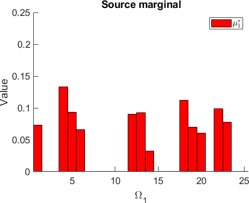
(a)

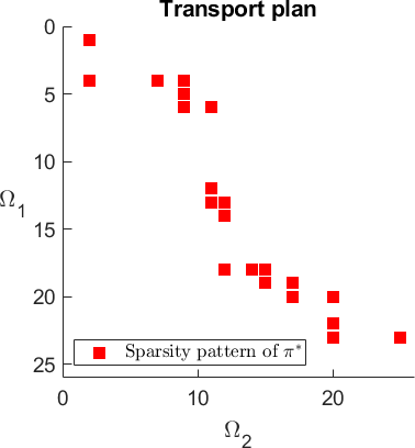
(b)

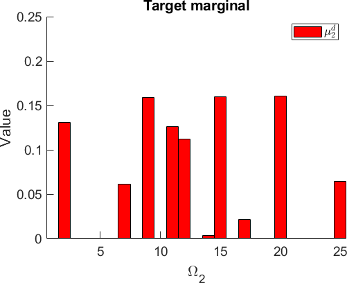
(c)

Figure 4.1. Randomly generated (semi-sparse) data. Figure 1(b) shows the sparsity pattern of the optimal transport plan $\pi^{*}$.

We then choose the observation domains $D_{1}=\Omega_{1}$ and $D=\Omega$, the exact observations $\mu_{1}^{\mathrm{d}}=\mu_{1}^{*}$ and $\pi_{\mathrm{d}}=\pi^{*}$, as well as the weight $\lambda=1$. As already mentioned, in this setting, the unique solution of the transportation identification problem (TI) is given by the couple $(\pi^{*},\mu_{1}^{*})$.

Figure 4.2 shows the evolution of the cluster point $\bar{\mu}_{1}$ of Algorithm 4.1 that we applied to solve the reduced transportation identification problem (RTI${}_{\gamma}^{\varepsilon}$) and Figure 4.3 shows the corresponding optimal transport plan $\bar{\pi}$ for different choices of the regularization parameters $\gamma$ and $\varepsilon$. For the constrained nonsmooth TR method, we chose the standard parameter configuration $R=\sqrt{n_{1}}$, $\Delta_{\min}=10^{-6}$, $\eta_{1}=0.1$, $\eta_{2}=0.9$, $\beta_{1}=0.5$, $\beta_{2}=1.5$, and $\nu=1$. The initial point and the initial TR radius were set to be $\mu_{1,0}={n_{1}}^{-1}\Mathbb{1}$ and $\Delta_{0}=1$, respectively, for every application of the method. We set the stationarity tolerance for the termination criterion in Step 5 to $\verb*|TOL|=10^{-5}$. This tolerance was achieved after a maximum of $70$ iterations in each test run shown.

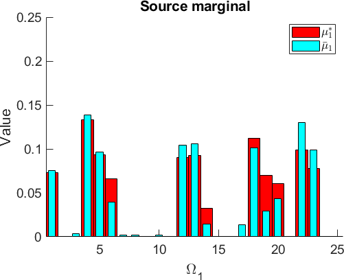
(a) $\gamma=\varepsilon=10^{-2}$

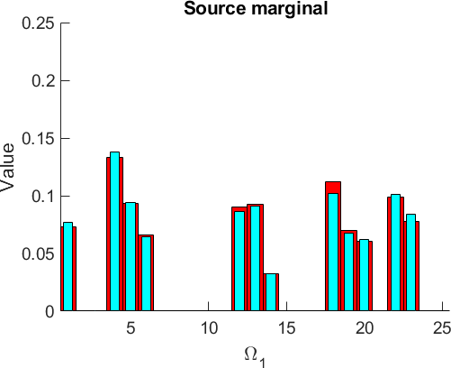
(b) $\gamma=\varepsilon=10^{-4}$

(c) $\gamma=\varepsilon=10^{-6}$

Figure 4.2. Estimated source marginal $\bar{\mu}_{1}$ (blue bars) compared to the “true” source marginal $\mu_{1}^{*}$ (red bars) for different values of regularization parameters $\gamma$ and $\varepsilon$.

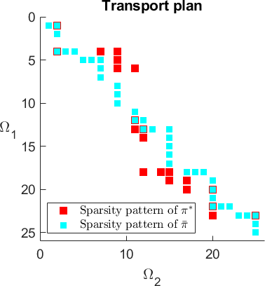
(a) $\gamma=\varepsilon=10^{-2}$

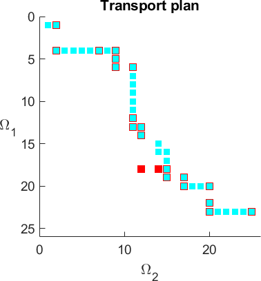
(b) $\gamma=\varepsilon=10^{-4}$

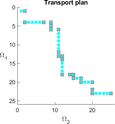
(c) $\gamma=\varepsilon=10^{-6}$

Figure 4.3. Comparison of the sparsity pattern (blue squares) of the optimal transport plans $\bar{\pi}$ corresponding to the estimated source marginals $\bar{\mu}_{1}$ from Figure 4.2 with the sparsity pattern (red squares) of the “true” optimal transport plan $\pi^{*}$ for different values of regularization parameters $\gamma$ and $\varepsilon$.

We observe that even with relatively large regularization parameters (i.e., $\gamma=\varepsilon=10^{-2})$ the source marginal $\mu_{1}^{*}$ is reasonably approximated, see Figure 2(a), and the quality of approximation becomes even better for declining regularization parameters, see Figure 2(b) – 2(c). When examining the corresponding optimal transport plans, it can be seen that the approximation is inaccurate for larger regularization parameters, but improves significantly up to a point where the sparsity pattern of $\pi^{*}$ is completely captured, see Figure 4.3. This (visual) observation is underpinned by the data given in Table 4.1.

$\gamma=\varepsilon$	$\max(\mu_{1}^{*}-\bar{\mu}_{1})$	$\max(\pi^{*}-\bar{\pi})$	$\mathcal{J}(\bar{\pi},\bar{\mu}_{1})$
$M^{M^{M}}$$10^{-2}$	$3.9855\cdot 10^{-2}$	$9.9722\cdot 10^{-2}$	$2.9307\cdot 10^{-2}$
$10^{-4}$	$1.0519\cdot 10^{-2}$	$8.9377\cdot 10^{-2}$	$2.6759\cdot 10^{-4}$
$10^{-6}$	$1.2200\cdot 10^{-4}$	$7.1756\cdot 10^{-5}$	$3.4216\cdot 10^{-8}$

Table 4.1. Collection of end-of-iteration data of the first numerical experiment for different values of regularization parameters $\gamma$ and $\varepsilon$.

For the second experiment, we reuse the data (i.e., the marginals, the cost matrix, and the optimal transport plan) from the first experiment but now consider different observation domains. In particular, we set $D_{1}=\{9,\dots,15\}$ and define $D$ to correspond to a band matrix with upper and lower bandwidth of $3$. The observed variables $\mu_{1}^{\mathrm{d}}$ and $\pi_{\mathrm{d}}$ are defined to be the restrictions of $\mu_{1}^{*}$ and $\pi^{*}$ to $D_{1}$ and $D$, respectively. Again, $(\pi^{*},\mu_{1}^{*})$ is a solution to the corresponding transportation identification problem (TI).

We again use the standard parameter configuration of the TR method. Similarly to before, Figure 4.4 shows the evolution of the cluster point $\bar{\mu}_{1}$ and Figure 4.5 shows the corresponding optimal transport plan $\bar{\pi}$ for different choices of the regularization parameters $\gamma$ and $\varepsilon$. In contrast to the previous experiment, the TR method exceeded the iteration limit of $200$ iterations in two of the three tests presented.

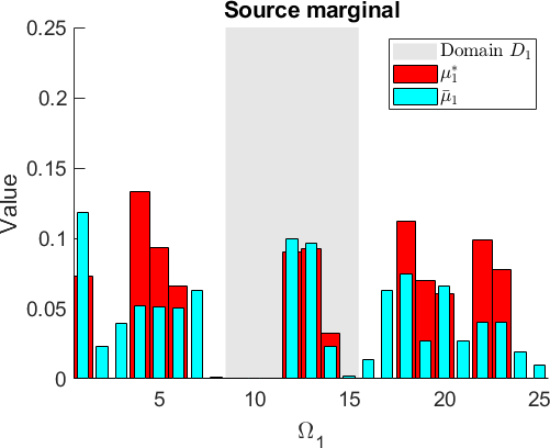
(a) $\gamma=\varepsilon=10^{-2}$

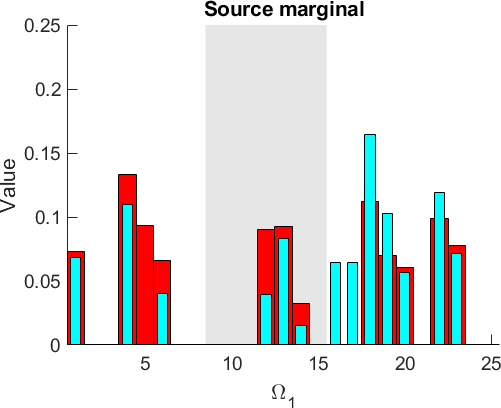
(b) $\gamma=\varepsilon=10^{-4}$

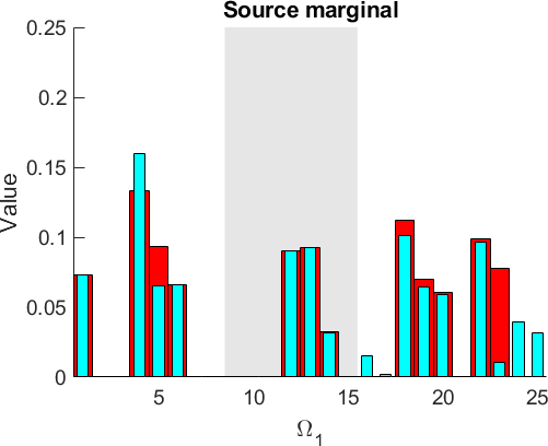
(c) $\gamma=\varepsilon=10^{-6}$

Figure 4.4. Estimated source marginal $\bar{\mu}_{1}$ (blue bars) compared to the “true” source marginal $\mu_{1}^{*}$ (red bars) for different values of regularization parameters $\gamma$ and $\varepsilon$. The gray region indicates the observation domain $D_{1}$.

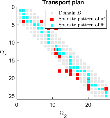
(a) $\gamma=\varepsilon=10^{-2}$

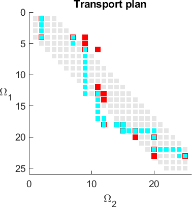
(b) $\gamma=\varepsilon=10^{-4}$

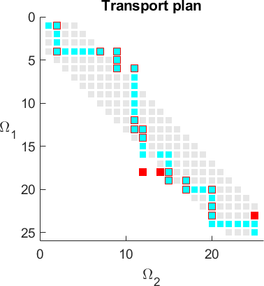
(c) $\gamma=\varepsilon=10^{-6}$

Figure 4.5. Comparison of the sparsity pattern (blue squares) of the optimal transport plans $\bar{\pi}$ corresponding to the estimated source marginals $\bar{\mu}_{1}$ from Figure 4.2 with the sparsity pattern (red squares) of the “true” optimal transport plan $\pi^{*}$ for different values of regularization parameters $\gamma$ and $\varepsilon$. The gray region indicates the observation domain $D$.

Again, we find that the quality of the approximation of both the source marginal and the corresponding optimal transport plan increases when the regularization parameters are reduced, see Table 4.2. Moreover, it seems that we can even (to some extent) approximate both variables outside the observation domain. We suspect that this behavior is due to the fact that the support of the transport plan $\pi^{*}$ lies to a large extent in the observation domain $D$ and that the relationship between marginals and transport plan is continuous. However, if we compare the objective function values of the two experiments, see the last columns of Table 4.1 and Table 4.2, we find that the quality of the approximation is several orders of magnitude worse in the latter case. However, this is not surprising since in the first experiment we had complete information (encoded in the objective function and its derivatives) about the source marginal and the optimal transportation plan, while in the second experiment there was a great lack of knowledge about the source marginal.

$\gamma=\varepsilon$	$\max(\mu_{1}^{*}-\bar{\mu}_{1})$	$\max(\pi^{*}-\bar{\pi})$	$\mathcal{J}(\bar{\pi},\bar{\mu}_{1})$
$M^{M^{M}}$$10^{-2}$	$8.1087\cdot 10^{-2}$	$9.9722\cdot 10^{-2}$	$2.7878\cdot 10^{-2}$
$10^{-4}$	$9.3342\cdot 10^{-2}$	$9.3342\cdot 10^{-2}$	$1.0152\cdot 10^{-2}$
$10^{-6}$	$6.6571\cdot 10^{-2}$	$6.4498\cdot 10^{-2}$	$3.1405\cdot 10^{-3}$

Table 4.2. Collection of end-of-iteration data of the second numerical experiment for different values of regularization parameters $\gamma$ and $\varepsilon$.

Appendix A Postponed Proofs

We now present the (rather technical) proofs of the lemmas that we have postponed from Subsection 2.3 to this Appendix. We start with the lemma that allows us to ”advance” the non-zero entry of a given matrix that is subject to a monotonic ordering without losing the existence of solutions to the corresponding system of inequations. We recall its formulation for the sake of clarity.

Lemma A.1 (Lemma 2.17 of Subsection 2.3).

We consider, for $p\in\{0,1\}$, the monotonic assignment functions $j_{p}\colon\Omega_{1}\to\Omega_{2}$, with $j_{p}(1)=1$, and denote their corresponding reduced system matrix and reduced cost vector by $A_{p}$ and $c_{p}$, respectively. Assume that $N\coloneqq j_{0}(n_{1})<n_{2}$ and that $j_{0}|_{\{1,\dots,n_{1}-1\}}\equiv j_{1}|_{\{1,\dots,n_{1}-1\}}$ as well as $j_{1}(n_{1})=j_{0}(n_{1})+1$.

Then, if the linear inequality system $A_{0}b\leq c_{0}$ has a solution, so does the linear inequality system $A_{1}b\leq c_{1}$.

Proof.

We have already examined the case that $N=1$ in Example 2.16 and therefore assume that $N\geq 2$. Let $d_{1}\in\mathbb{R}^{n_{1}(n_{2}-1)}$ be a solution to the linear system $A_{1}^{\top}d=0$ with $d_{1}\geq 0$. We then define the vector $d_{0}\in\mathbb{R}^{n_{1}(n_{2}-1)}$ by

$$\begin{split}&d^{(i_{1}-1)(n_{2}-1)+i_{2}}_{0}\\ &\quad\coloneqq\begin{cases}d^{(i_{1}-1)(n_{2}-1)+N-1}_{1}+d^{(i_{1}-1)(n_{2}-1)+N}_{1},&\text{if}~{}i_{1}\notin j_{0}^{-1}(N)~{}\text{and}~{}i_{2}=N-1,\\ 0,&\text{if}~{}i_{2}=N,\\ d^{(i_{1}-1)(n_{2}-1)+i_{2}}_{1},&\text{else},\end{cases}\end{split}$$ (A.1)

for all $i_{1}\in\{1,\dots,n_{1}\}$ and $i_{2}\in\{1,\dots,n_{2}-1\}$. In the following, we will show that $d_{0}$ is a solution to the linear system $A_{0}^{\top}d=0$.

By construction, $d_{0}\geq 0$ and

$$\sum_{i_{2}=1}^{n_{2}-1}d^{(i_{1}-1)(n_{2}-1)+i_{2}}_{0}=\sum_{i_{2}=1}^{n_{2}-1}d^{(i_{1}-1)(n_{2}-1)+i_{2}}_{1}\quad\text{for all}~{}i_{1}\notin j_{0}^{-1}(N).$$ (A.2)

For $p\in\{0,1\}$, the structure of the reduced system matrices $A_{p}$ yields that

$$\begin{split}\bigl{(}A_{p}^{\top}d_{p}\bigr{)}_{l}&=\sum_{i_{1}\colon j_{p}(i_{1})<l}d^{(i_{1}-1)(n_{2}-1)+l-1}_{p}\\ &\quad+\sum_{i_{1}\colon j_{p}(i_{1})=l}\sum_{i_{2}=1}^{n_{2}-1}-d^{(i_{1}-1)(n_{2}-1)+i_{2}}_{p}\\ &\quad+\sum_{i_{1}\colon j_{p}(i_{1})>l}d^{(i_{1}-1)(n_{2}-1)+l}_{p}\end{split}$$ (A.3)

for all $l\in\Omega_{2}$. If follows from the definition of $j_{1}$ that

$$\begin{split}&\{i_{1}\colon j_{0}(i_{1})<l\}=\{i_{1}\colon j_{1}(i_{1})<l\},\\ &\{i_{1}\colon j_{0}(i_{1})=l\}=\{i_{1}\colon j_{1}(i_{1})=l\},\hskip 20.00003pt\text{for all}~{}l\in\{1,\dots,N-1\}.\\ &\{i_{1}\colon j_{0}(i_{1})>l\}=\{i_{1}\colon j_{1}(i_{1})>l\},\end{split}$$ (A.4)

For $l\in\{1,\dots,N-2\}$ it holds that $j_{0}^{-1}(l)\cap j_{0}^{-1}(N)=\emptyset$. We thus use (A.1) – (A.4) to find that

$$(A_{0}^{\top}d_{0})_{l} =\sum_{i_{1}\colon j_{1}(i_{1})<l}d^{(i_{1}-1)(n_{2}-1)+l-1}_{1}$$

$$\quad+\sum_{i_{1}\colon j_{1}(i_{1})=l}\sum_{i_{2}=1}^{n_{2}-1}-d^{(i_{1}-1)(n_{2}-1)+i_{2}}_{1}$$

$$\quad+\sum_{i_{1}\colon j_{1}(i_{1})>l}d^{(i_{1}-1)(n_{2}-1)+l}_{1}=(A_{1}^{\top}d_{1})_{l}=0,$$

where the last equality follows from the assumption on $d_{1}$. We moreover find that

$$\{i_{1}\colon j_{0}(i_{1})\leq N-1\}\,\cap\,j_{0}^{-1}(N)=\emptyset\quad\text{and}\quad\{i_{1}\colon j_{0}(i_{1})>N-1\}=j_{0}^{-1}(N),$$ (A.5)

since $j_{0}$ is monotone and $N=j_{0}(n_{1})$. Similarly to before, we use (A.1) – (A.5) to obtain that

$$(A_{0}^{\top}d_{0})_{N-1} =\sum_{i_{1}\colon j_{1}(i_{1})<N-1}d^{(i_{1}-1)(n_{2}-1)+N-2}_{1}$$

$$\quad+\sum_{i_{1}\colon j_{1}(i_{1})=N-1}\sum_{i_{2}=1}^{n_{2}-1}-d^{(i_{1}-1)(n_{2}-1)+i_{2}}_{1}$$

$$\quad+\sum_{i_{1}\colon j_{1}(i_{1})>N-1}d^{(i_{1}-1)(n_{2}-1)+N-1}_{1}=(A_{1}^{\top}d_{1})_{N-1}=0.$$

By the properties of $j_{0}$, it holds that $\Omega_{1}=\{i_{1}\colon j_{0}(i_{1})<N\}~{}\dot{\cup}~{}j_{0}^{-1}(N)$ and therefore $\{i_{1}\colon j_{0}(i_{1})>N\}=\emptyset$. Thus, we again use (A.1) and (A.3) to calculate that

$$(A_{0}^{\top}d_{0})_{N}$$

$$\quad=\sum_{i_{1}\notin j_{0}^{-1}(N)}\bigl{(}d^{(i_{1}-1)(n_{2}-1)+N-1}_{1}+d^{(i_{1}-1)(n_{2}-1)+N}_{1}\bigr{)}$$

$$\qquad+\sum_{i_{1}\in j_{0}^{-1}(N)}\sum_{i_{2}=1}^{n_{2}-1}-d^{(i_{1}-1)(n_{2}-1)+i_{2}}_{0}$$

$$\quad=d_{1}^{N-1}+d_{1}^{N}+\sum_{i_{1}\in\{2,\dots,n_{1}\}\setminus j_{0}^{-1}(N)}\bigl{(}d^{(i_{1}-1)(n_{2}-1)+N-1}_{1}+d^{(i_{1}-1)(n_{2}-1)+N}_{1}\bigr{)}$$

$$\qquad+\sum_{i_{1}\in j_{0}^{-1}(N)}d^{(i_{1}-1)(n_{2}-1)+N}_{1}+\sum_{i_{1}\in j_{0}^{-1}(N)}-d^{(i_{1}-1)(n_{2}-1)+N}_{1}$$

$$\qquad+\sum_{i_{1}\in j_{0}^{-1}(N)}\sum_{i_{2}\in\{1,\dots,n_{2}-1\}\setminus\{N\}}-d^{(i_{1}-1)(n_{2}-1)+i_{2}}_{1}$$

$$\quad=d_{1}^{N-1}+d_{1}^{N}+\sum_{i_{1}\in\{2,\dots,n_{1}\}\setminus j_{0}^{-1}(N)}d^{(i_{1}-1)(n_{2}-1)+N-1}_{1}+r_{1}+r_{2},$$

with

$$r_{1} =\sum_{i_{1}\in\{2,\dots,n_{1}\}\setminus j_{0}^{-1}(N)}d^{(i_{1}-1)(n_{2}-1)+N}_{1}+\sum_{i_{1}\in j_{0}^{-1}(N)}d^{(i_{1}-1)(n_{2}-1)+N}_{1}$$

$$=\sum_{i_{1}=2}^{n_{1}-1}d^{(i_{1}-1)(n_{2}-1)+N}_{1}+d^{(n_{1}-1)(n_{2}-1)+N}_{1}$$

and

$$r_{2} =\sum_{i_{1}\in j_{0}^{-1}(N)}-d^{(i_{1}-1)(n_{2}-1)+N}_{1}+\sum_{i_{1}\in j_{0}^{-1}(N)}\sum_{i_{2}\in\{1,\dots,n_{2}-1\}\setminus\{N\}}-d^{(i_{1}-1)(n_{2}-1)+i_{2}}_{1}$$

$$=\sum_{i_{1}\in j_{0}^{-1}(N)\setminus\{n_{1}\}}\sum_{i_{2}=1}^{n_{2}-1}-d^{(i_{1}-1)(n_{2}-1)+i_{2}}_{1}+\sum_{i_{2}=1}^{n_{2}-1}-d^{(n_{1}-1)(n_{2}-1)+i_{2}}_{1}.$$

Further, taking a close look at the linear system $A_{1}^{\top}d_{1}=0$, we find that

$$\sum_{i_{1}\in\{2,\dots,n_{1}\}\setminus j_{0}^{-1}(N)}d^{(i_{1}-1)(n_{2}-1)+N-1}_{1}+r_{1}+r_{2}$$

$$\quad=-\biggl{(}\sum_{i_{1}\in\{2,\dots,n_{1}\}\setminus j_{0}^{-1}(N)}-d^{(i_{1}-1)(n_{2}-1)+N-1}_{1}$$

$$\qquad\quad-d^{(n_{1}-1)(n_{2}-1)+N}_{1}+\sum_{i_{1}\in j_{0}^{-1}(N)\setminus\{n_{1}\}}\sum_{i_{2}=1}^{n_{2}-1}d^{(i_{1}-1)(n_{2}-1)+i_{2}}_{1}\biggr{)}$$

$$\qquad-\biggl{(}\sum_{i_{1}=2}^{n_{1}-1}-d^{(i_{1}-1)(n_{2}-1)+N}_{1}+\sum_{i_{2}=1}^{n_{2}-1}d^{(n_{1}-1)(n_{2}-1)+i_{2}}_{1}\biggr{)}$$

$$\quad=-d_{1}^{N-1}-d_{1}^{N}$$

and consequently $(A_{0}^{\top}d_{0})_{N}=0.$ Because of $\{i_{1}\colon j_{0}(i_{1})<N+1\}=\Omega_{1}$, we immediately receive from (A.1) and (A.3) that

$$(A_{0}^{\top}d_{0})_{N+1}=\sum_{i_{1}\colon j_{0}(i_{1})<N+1}d^{(i_{1}-1)(n_{2}-1)+N}_{0}=0.$$

Similarly, for $l\in\{N+2,\dots,n_{2}\}$, we find that

$$(A_{0}^{\top}d_{0})_{l}=\sum_{i_{1}\colon j_{0}(i_{1})<l}d^{(i_{1}-1)(n_{2}-1)+l-1}_{0}=\sum_{i_{1}=1}^{n_{1}}d^{(i_{1}-1)(n_{2}-1)+l-1}_{1}=0,$$

where the last equality again can be deduced from the linear system $A_{1}^{\top}d_{1}=0$. Im summary, we have shown that $A_{0}^{\top}d_{0}=0$.

Now, assume that the system $A_{0}b\leq c_{0}$ has a solution. Then by Farka’s lemma, $d_{0}^{\top}c_{0}\geq 0$. Comparing $c_{0}$ with $c_{1}$ yields that

$$\begin{split}&c^{(i_{1}-1)(n_{2}-1)+i_{2}}_{1}\\ &\quad=c^{(i_{1}-1)(n_{2}-1)+i_{2}}_{0}+\begin{cases}0,&\text{if}~{}i_{1}\leq n_{1}-1,\\ 2\,\bigl{(}c_{\mathrm{d}}^{n_{1},N}-c_{\mathrm{d}}^{n_{1},N+1}\bigr{)},&\text{if}~{}i_{1}=n_{1}~{}\text{and}~{}i_{2}=N,\\ c_{\mathrm{d}}^{n_{1},N}-c_{\mathrm{d}}^{n_{1},N+1},&\text{else},\end{cases}\end{split}$$ (A.6)

for all $i_{1}\in\Omega_{1}$ and $i_{2}\in\Omega_{2}\setminus\{n_{2}\}$, see (2.4). Moreover,

$$c^{(i_{1}-1)(n_{2}-1)+N}_{1}=c_{\mathrm{d}}^{i_{1},N+1}-c_{\mathrm{d}}^{i_{1},j_{0}(i_{1})}\quad\text{for all}~{}i_{1}\in\Omega_{1}\setminus\{n_{1}\},$$

whereas

$$c^{(n_{1}-1)(n_{2}-1)+N}_{1}=c_{\mathrm{d}}^{n_{1},N}-c_{\mathrm{d}}^{n_{1},N+1},$$

and

$$c^{(i_{1}-1)(n_{2}-1)+N-1}_{1}=c_{\mathrm{d}}^{i_{1},N}-c_{\mathrm{d}}^{i_{1},j_{0}(i_{1})}\quad\text{for all}~{}i_{1}\notin j_{0}^{-1}(N).$$

This, together with the definition of $d_{0}$ from (A.1) and (A.6) leads to

$$\begin{split}&d_{1}^{\top}c_{1}-d_{0}^{\top}c_{0}\\ &\quad=\sum_{i_{1}\notin j_{0}^{-1}(N)}d^{(i_{1}-1)(n_{2}-1)+N}_{1}\bigl{(}c^{(i_{1}-1)(n_{2}-1)+N}_{1}-c^{(i_{1}-1)(n_{2}-1)+N-1}_{1}\bigr{)}\\ &\qquad+\sum_{i_{1}\in j_{0}^{-1}(N)\setminus\{n_{1}\}}d^{(i_{1}-1)(n_{2}-1)+N}_{1}c^{(i_{1}-1)(n_{2}-1)+N}_{1}\\ &\qquad+\sum_{i_{2}\in\{1,\dots,n_{2}-1\}\setminus\{N\}}d^{(n_{1}-1)(n_{2}-1)+i_{2}}_{1}\bigl{(}c^{(n_{1}-1)(n_{2}-1)+i_{2}}_{1}-c^{(n_{1}-1)(n_{2}-1)+i_{2}}_{0}\bigr{)}\\ &\qquad+d^{(n_{1}-1)(n_{2}-1)+N}_{1}\,c^{(n_{1}-1)(n_{2}-1)+N}_{1}\\ &\quad=\sum_{i_{1}=1}^{n_{1}-1}d^{(i_{1}-1)(n_{2}-1)+N}_{1}\bigl{(}c_{\mathrm{d}}^{i_{1},N+1}-c_{\mathrm{d}}^{i_{1},N}\bigr{)}\\ &\qquad+\sum_{i_{2}=1}^{n_{2}-1}d^{(n_{1}-1)(n_{2}-1)+i_{2}}_{1}\bigl{(}c_{\mathrm{d}}^{n_{1},N}-c_{\mathrm{d}}^{n_{1},N+1}\bigr{)}.\end{split}$$ (A.7)

The equation $(A_{1}^{\top}d_{1})_{N+1}=0$ reveals that

$$\sum_{i_{1}=1}^{n_{1}-1}d^{(i_{1}-1)(n_{2}-1)+N}_{1}=\sum_{i_{2}=1}^{n_{2}-1}d^{(n_{1}-1)(n_{2}-1)+i_{2}}_{1},$$

which, if plugged into the equation in (A.7), yields that

$$d_{1}^{\top}c_{1}-d_{0}^{\top}c_{0} =\sum_{i_{1}=1}^{n_{1}-1}d^{(i_{1}-1)(n_{2}-1)+N}_{1}\bigl{(}c_{\mathrm{d}}^{i_{1},N+1}-c_{\mathrm{d}}^{i_{1},N}-(c_{\mathrm{d}}^{n_{1},N+1}-c_{\mathrm{d}}^{n_{1},N})\bigr{)}\geq 0,$$

where the nonnegativity stems from the assumption that $d_{1}\geq 0$ and Lemma 2.14 (for $i_{2}=N+1$). Consequently, $d_{1}^{\top}c_{1}\geq d_{0}^{\top}c_{0}\geq 0$ which, owing to Farka’s lemma, completes the proof. ∎

It remains to prove the lemma that allows us to “move up” the non-zero entries of the rows above.

Lemma A.2 (Lemma 2.18 of Subsection 2.3).

For $n_{2}\geq n_{1}\geq 3$ and $p\in\{0,1\}$, consider the monotonic assignment functions $j_{p}\colon\Omega_{1}\to\Omega_{2}$ with $j_{p}(1)=1$ and denote their corresponding reduced system matrix and reduced cost vector by $A_{p}$ and $c_{p}$, respectively. Assume that $N\coloneqq j_{0}(n_{1})\geq 2$, abbreviate $I\coloneqq\max\{i_{1}\in\Omega_{1}\colon i_{1}\notin j_{0}^{-1}(N)\}$, and, moreover, assume that $I>1$, $j_{0}(I)=N-1$, $j_{0}|_{\Omega_{1}\setminus\{I\}}\equiv j_{1}|_{\Omega_{1}\setminus\{I\}}$, as well as $j_{1}(I)=N=j_{0}(I)+1$.

Then, if the linear inequality system $A_{0}b\leq c_{0}$ has a solution, so does the linear inequality system $A_{1}b\leq c_{1}$.

Proof.

Let us assume that the linear system $A_{0}b\leq c_{0}$ given by

$$b_{i_{2}}-b_{j_{0}(i_{1})}\leq c_{\mathrm{d}}^{i_{1},i_{2}}-c_{\mathrm{d}}^{i_{1},j_{0}(i_{1})}\quad\text{for all}~{}i_{1}\in\Omega_{1},~{}i_{2}\in\Omega_{2}\setminus\{j_{0}(i_{1})\},$$

has a solution. Then obviously, the subsystem

$$b_{i_{2}}-b_{j_{0}(i_{1})}\leq c_{\mathrm{d}}^{i_{1},i_{2}}-c_{\mathrm{d}}^{i_{1},j_{0}(i_{1})}\quad\text{for all}~{}i_{1}\in\{1,\dots,I\},~{}i_{2}\in\Omega_{2}\setminus\{j_{0}(i_{1})\},$$

has the same solution. We apply Lemma 2.17 to the restriction $j_{0}|_{\{1,\dots,I\}}$ to find that the system

$$b_{i_{2}}-b_{j_{1}(i_{1})}\leq c_{\mathrm{d}}^{i_{1},i_{2}}-c_{\mathrm{d}}^{i_{1},j_{1}(i_{1})}\quad\text{for all}~{}i_{1}\in\{1,\dots,I\},~{}i_{2}\in\Omega_{2}\setminus\{j_{1}(i_{1})\},$$ (A.8)

with $j_{1}|_{\{1,\dots,I-1\}}\equiv j_{0}|_{\{1,\dots,I-1\}}$ and $j_{1}(I)=j_{0}(I)+1=N$, admits a solution $b^{\prime}\in\mathbb{R}^{n_{2}}$, which we then use to define the vector $b_{1}\in\mathbb{R}^{n_{2}}$ by

$$b_{1}^{i_{2}}\coloneqq b_{i_{2}}^{\prime}-\begin{cases}0,&\text{if}~{}i_{2}\leq N,\\ c_{\mathrm{d}}^{I,i_{2}}-c_{\mathrm{d}}^{I,N}-(c_{\mathrm{d}}^{n_{1},i_{2}}-c_{\mathrm{d}}^{n_{1},N}),&\text{if}~{}i_{2}>N,\end{cases}$$

for all $i_{2}\in\Omega_{2}$.

Let $i_{1}\in\{1,\dots,I-1\}$ and $i_{2}\in\Omega_{2}\setminus\{j_{1}(i_{1})\}$ be arbitrary. By construction of $j_{1}$, it holds that $j_{1}(i_{1})<N$. If $i_{2}\leq N$, then because $b^{\prime}$ satisfies (A.8) we find that

$$b_{1}^{i_{2}}-b_{1}^{j_{1}(i_{1})}=b_{i_{2}}^{\prime}-b_{j_{1}(i_{1})}^{\prime}\leq c_{\mathrm{d}}^{i_{1},i_{2}}-c_{\mathrm{d}}^{i_{1},j_{1}(i_{1})}.$$

If $i_{2}>N$, we additionally apply Lemma 2.14 to receive

$$b_{1}^{i_{2}}-b_{1}^{j_{1}(i_{1})} =b_{i_{2}}^{\prime}-\bigl{(}c_{\mathrm{d}}^{I,i_{2}}-c_{\mathrm{d}}^{I,N}-(c_{\mathrm{d}}^{n_{1},i_{2}}-c_{\mathrm{d}}^{n_{1},N})\bigr{)}-b_{j_{1}(i_{1})}^{\prime}$$

$$\leq b_{i_{2}}^{\prime}-b_{j_{1}(i_{1})}^{\prime}\leq c_{\mathrm{d}}^{i_{1},i_{2}}-c_{\mathrm{d}}^{i_{1},j_{1}(i_{1})}.$$

The other case, i.e., $i_{1}\in\{I,\dots,n_{1}\}$, can be discussed analogously and is therefore omitted.

Altogether, we have shown that

$$b_{1}^{i_{2}}-b_{1}^{j_{1}(i_{1})}\leq c_{\mathrm{d}}^{i_{1},i_{2}}-c_{\mathrm{d}}^{i_{1},j_{1}(i_{1})}$$

for all $i_{1}\in\Omega_{1}$ and all $i_{2}\in\Omega_{2}\setminus\{j_{1}(i_{1})\}$, as claimed. ∎

References

• [1] Francisco Andrade, Gabriel Peyre and Clarice Poon “Sparsistency for Inverse Optimal Transport” In arXiv preprint arXiv:2310.05461, 2023
• [2] Marcello Carioni, José A Iglesias and Daniel Walter “Extremal Points and Sparse Optimization for Generalized Kantorovich–Rubinstein Norms” In Foundations of Computational Mathematics Springer, 2023, pp. 1–42
• [3] Eduardo Casas, Christian Clason and Karl Kunisch “Approximation of elliptic control problems in measure spaces with sparse solutions” In SIAM J. Control Optim. 50.4, 2012, pp. 1735–1752
• [4] Eduardo Casas and Karl Kunisch “Optimal control of semilinear elliptic equations in measure spaces” In SIAM J. Control Optim. 52.1, 2014, pp. 339–364
• [5] Eduardo Casas and Karl Kunisch “Optimal control of the two-dimensional stationary Navier-Stokes equations with measure valued controls” In SIAM J. Control Optim. 57.2, 2019, pp. 1328–1354
• [6] Wei-Ting Chiu, Pei Wang and Patrick Shafto “Discrete probabilistic inverse optimal transport” In International Conference on Machine Learning, 2022, pp. 3925–3946 PMLR
• [7] Constantin Christof, Juan Carlos De los Reyes and Christian Meyer “A nonsmooth trust-region method for locally Lipschitz functions with application to optimization problems constrained by variational inequalities” In SIAM J. Optim. 30.3, 2020, pp. 2163–2196 DOI: 10.1137/18M1164925
• [8] Frank H Clarke “Optimization and nonsmooth analysis” SIAM, 1990
• [9] Christian Clason, Dirk A. Lorenz, Hinrich Mahler and Benedikt Wirth “Entropic regularization of continuous optimal transport problems” In J. Math. Anal. Appl. 494.1, 2021, pp. Paper No. 124432\bibrangessep22 DOI: 10.1016/j.jmaa.2020.124432
• [10] Marco Cuturi “Sinkhorn distances: Lightspeed computation of optimal transport” In Advances in neural information processing systems, 2013, pp. 2292–2300
• [11] Lester Randolph Ford “Flows in networks” Princeton university press, 2015
• [12] Sebastian Hillbrecht “A Quadratic Regularization of Optimal Transport Problems and Its Application to Bilevel Optimization”, 2024 DOI: http://dx.doi.org/10.17877/DE290R-24300
• [13] Sebastian Hillbrecht and Christian Meyer “Bilevel Optimization of the Kantorovich Problem and its Quadratic Regularization Part I: Existence Results” arXiv:2206.13220, 2022
• [14] Sebastian Hillbrecht, Christian Meyer and Paul Manns “Bilevel Optimization of the Kantorovich Problem and its Quadratic Regularization Part II: Convergence Analysis” arXiv:2211.07287, 2022
• [15] Michael Hintermüller and Thomas Surowiec “A Bundle-Free Implicit Programming Approach for a Class of Elliptic MPECs in Function Space” In Math. Program. 160.1–2, 2016, pp. 271–305
• [16] Leonid V. Kantorovič “On the translocation of masses” In C. R. (Doklady) Acad. Sci. URSS (N.S.) 37, 1942, pp. 199–201
• [17] Michal Kočvara “Topology optimization with displacement constraints: a bilevel programming approach” In Structural optimization 14 Springer, 1997, pp. 256–263
• [18] Dirk A. Lorenz, Paul Manns and Christian Meyer “Quadratically regularized optimal transport” In Appl. Math. Optim. 83.3, 2021, pp. 1919–1949 DOI: 10.1007/s00245-019-09614-w
• [19] David G Luenberger and Yinyu Ye “Linear and nonlinear programming” Springer, 1984
• [20] Konstantin Pieper and Boris Vexler “A priori error analysis for discretization of sparse elliptic optimal control problems in measure space” In SIAM Journal on Control and Optimization 51.4 SIAM, 2013, pp. 2788–2808
• [21] Filippo Santambrogio “Optimal transport for applied mathematicians” Calculus of variations, PDEs, and modeling 87, Progress in Nonlinear Differential Equations and their Applications Birkhäuser/Springer, Cham, 2015 DOI: 10.1007/978-3-319-20828-2
• [22] Alexander Shapiro “On concepts of directional differentiability” In Journal of optimization theory and applications 66 Springer, 1990, pp. 477–487
• [23] Andrew M Stuart and Marie-Therese Wolfram “Inverse optimal transport” In SIAM Journal on Applied Mathematics 80.1 SIAM, 2020, pp. 599–619
• [24] Cédric Villani “Optimal transport. Old and new” 338, Grundlehren der Mathematischen Wissenschaften [Fundamental Principles of Mathematical Sciences] Springer-Verlag, Berlin, 2009 DOI: 10.1007/978-3-540-71050-9
• [25] Cédric Villani “Topics in optimal transportation” 58, Graduate Studies in Mathematics American Mathematical Society, Providence, RI, 2003 DOI: 10.1007/b12016