On the block size spectrum of the multiplicative Beta coalescent

Abstract.

In this work we introduce the dynamic $\Lambda$-random graph and the associated multiplicative $\Lambda$-coalescent. The dynamic $\Lambda$-random graph is an exchangeable and consistent random graph process, inspired by the classical $\Lambda$-coalescent studied in mathematical population genetics. Our main concern is the multiplicative $\Lambda$-coalescent, which accounts for the connected components (blocks) of the graph. This process is exchangeable but not consistent. We focus on the case where $\Lambda$ is the beta measure and prove a dynamic law of large numbers for the block size spectrum, which tracks the numbers of blocks containing $1,...,d$ elements. On top of that, we provide a functional limit theorem for the fluctuations around its deterministic trajectory. The limit process satisfies a stochastic differential equation of Ornstein-Uhlenbeck type.

Keywords: coalescent process, random graphs, functional limit theorem, Poisson representation, Ornstein-Uhlenbeck type process.

MSC 2020 classification: Primary: 60J90, Secondary: 05C80, 60F17, 60F15.

1. Introduction

The study of random graphs and networks is an active and rapidly developing area of research [29, 10]. In addition to their rich mathematical structure, random networks find applications in a large number of fields such as biology [18], sociology [14], neuroscience [7], computer science [6], and more.

The perhaps most canonical example of a random graph is that of Erdős and Rényi, by now known as the Erdős-Rényi random graph model  [12, 13]; see for example [16] for more details about random graphs. In that model, a random number of edges is drawn, connecting each pair of edges with a fixed probability. After proper rescaling, the connected components can be described by means of excursions of a Brownian motion with drift [1]. Dynamic versions of this model, in which vertices are connected by edges arriving at exponential waiting times, have been investigated as well. It was shown that, after letting the total number of vertices tend to infinity, slowing down time and normalising appropriately, the behaviour of the frequencies of small connected components is captured by a deterministic ordinary differential equation, known as Smoluchowski’s coagulation equation [15].

By restricting attention to their connected components and ignoring the rest of the graph structure, dynamic random graph models give rise in a natural way to coalescent processes, i.e. stochastic processes that take values in the set of partitions (or, equivalently, equivalence relations) of the set of vertices by declaring two vertices equivalent if they are connected via some path in the graph [4]. For instance, the evolution of the components of the dynamic Erdős-Rényi model is known as the multiplicative coalescent [1, 5, 21]. Another coalescent process that can be interpreted via an underlying random graph is the additive coalescent, treated alongside the multiplicative case in [5].

To a large degree, the interest in coalescent processes is due to their application in mathematical population genetics [30]. There, the goal is usually to describe the backward-in-time evolution of the genealogy of a sample of genes taken at present; as one looks further and further into the past, sets/blocks of samples are merged to indicate identity by descent. Owing to biological reality, a main focus has traditionally been on coalescent processes that are exchangeable in the sense that they should be insensitive to arbitrary reordering of labels, and consistent in the sense that the coalescent associated with a subsample should agree with the marginal of the coalescent of the full sample. In 1999, Pitman [24] and Sagitov [26] independently classified all such coalescents with asynchronous mergers by showing them to be in one-to-one correspondence with finite measures on $[0,1]$. Later, Schweinsberg [27] generalised this classification to allow for simultaneous mergers.

By incorporating types one can weaken the usual notion of exchangeability to partial exchangeability. Johnston, Rogers and Kyprianou [17] gave a classification of such coalescents analogous to the one in [24, 26] for the exchangeable case.

A natural extension is to drop (or at least to weaken) the assumption of consistency. One way to do this is to consider coalescent processes that may not be consistent themselves, but are associated with consistent, exchangeable random graph processes. Although a classification of such random graph processes was given in [8], a detailed investigation of their properties has yet to be carried out.

As a prototypical example, we consider in this work a dynamic random graph model that is associated with a finite measure $\Lambda$ in a similar way as the classical coalescents in [24, 26, 9]. Put simply, in the classical $\Lambda$-coalescent one observes $u$ mergers at rate $\Lambda({\,\rm d}u)/u^{2}<\infty$, in which each block participates independently with probability $u$. This choice of $\Lambda$ guarantees that we observe transitions at a finite rate when considering finitely many blocks, resulting in a well-defined coalescent process.

In our work we consider a random graph model in which, at rate $\Lambda({\,\rm d}u)/u^{2}$, a large community is created by connecting a proportion of vertices with a complete graph. Leaving a more detailed exploration of its structure to future work, we investigate the associated coalescent, which we call the multiplicative $\Lambda$-coalescent. The qualifier ‘multiplicative’ is due to the fact that the effective merging rates for different blocks is proportional to the product of their sizes. This is in contrast to the classical $\Lambda$-coalescent, where the merging rate is independent of the block sizes. We stress that our model is different from that treated in [20]. While that paper also considers an extension of the multiplicative coalescent with multiple mergers, the family sizes stay bounded as the number of vertices increases, resulting in a non-consistent random graph process. In our model, family sizes are a positive fraction of the total number of vertices.

In line with the tradition in population genetics, we will focus on the special case, where $\Lambda$ is the Beta distribution; this allows for nice, explicit computations, although we expect our results to also hold in (slightly) greater generality. Similar to [23], we derive a dynamic law of large numbers for the number of connected components containing $1,...,d$ elements, see Remark 2.1. We also prove a non-standard functional limit for the fluctuations around this deterministic limit. Our results mirrors that of [22] on the fluctuations of the total number of blocks in the $\Lambda$-coalescent when $\Lambda$ looks like a Beta distribution around the origin. More details can be found in Remark 2.3.

The rest of the paper is organised as follows. After introducing our model and stating our main results in Section 2, we start Section 3 by adapting the Poisson integral representation from [22] to our setting, which will be the central tool for our proof. These kind of representations are reminiscent of those used in [19] or [11]. Right after, we give an overview over the structure of the proof before diving into the technical details. Finally, in Section 4, we recall some useful results from real analysis that are used elsewhere in the text.

2. Model and main results

2.1. The dynamic $\Lambda$-random graph and its (finite) block spectrum

We start this section by introducing the main objects and stating our two main results. We define a Markov process $G^{n}=(G^{n}_{t})_{t\geqslant 0}$ taking values in the set of (undirected) graphs with vertices $[n]\mathrel{\mathop{:}}=\{1,\ldots,n\}$ and dynamically evolving edges.

Definition 2.1 ($\Lambda$-dynamic random graph).

Let $\Lambda$ be a finite measure on $(0,1]$ and let $N$ be a Poisson point process on $[0,\infty)\times(0,1]$ with intensity

$$\mu({\,\rm d}t,{\,\rm d}u)\mathrel{\mathop{:}}={\,\rm d}t\frac{\Lambda({\,\rm d}u)}{u^{2}}.$$ (2.1)

For each atom $(t,u)$ of $N$ we colour at time $t$ each vertex independently with probability $u$ and subsequently connect all pairs of coloured vertices.

Denoting by $E^{n}_{t}\subseteq[n]^{2}$ the set of edges of $G^{n}$ at time $t$, we set for each atom $(t,u)$ of $N$

$$E_{t}^{n}\mathrel{\mathop{:}}=E_{t-}^{n}\cup\big{\{}\{i,j\}:i,j\in[n],i\neq j,B_{i}=B_{j}=1\big{\}},$$ (2.2)

where $B_{1},\ldots,B_{n}$ are independent Bernoulli random variables with success probability $u$, i.e. we consider $i\in[n]$ to be coloured if and only if $B_{i}=1$. We call the resulting graph-valued Markov process $G^{n}$ the $\Lambda$-dynamic random graph on $n$ vertices; see Figure 1 for an illustration.

In general $G_{0}^{n}$ might be any graph with $n$ vertices, however in our case we usually consider $G_{0}^{n}=([n],\varnothing)$. Note that this defines a consistent family $G_{n}$ of exchangeable dynamic random graphs.

Figure 1. An illustration of two consecutive transitions of the $\Lambda$-graph on $16$ vertices. Left: a given state of the graph; the green vertices are selected to be connected via a complete graph. Middle: the graph after the first transition; the superposed complete graph is depicted bold; the green vertices are selected to be connected. Right: the graph after the second transition; the superposed graph is depicted bold. The associated multiplicative $\Lambda$-coalescent performs the transitions:
$\text{ }\qquad\qquad\qquad\{\{1\},\{2,13\},\{{\color[rgb]{0,0.9,0}3},5,6\},\{4\},\{7\},\{8\},\{9,14,15,{\color[rgb]{0,0.9,0}16}\},\{10\},\{{\color[rgb]{0,0.9,0}11}\},\{{\color[rgb]{0,0.9,0}12}\}$
$\text{ }\qquad\qquad\qquad\qquad\to\{\{1\},\{2,{\color[rgb]{0,0.9,0}13}\},\{3,5,6,9,11,12,14,15,16\},\{{\color[rgb]{0,0.9,0}4}\},\{7\},\{{\color[rgb]{0,0.9,0}8}\},\{10\}\}$
$\text{ }\qquad\qquad\qquad\qquad\qquad\to\{\{1\},\{2,4,8,13\},\{3,5,6,9,11,12,14,15,16\},\{7\},\{10\}\}.$

Note that the second set on the right-hand side of Eq. (2.2) is almost surely empty outside of a locally finite set of $t\in[0,\infty)$. Therefore, this indeed defines a Markov process with càdlàg paths on the set of undirected graphs with $n$ vertices, if the latter is endowed with the discrete topology.

It is natural to associate with $G^{n}$ a coalescent process, i.e. a Markov process taking values in the partitions of $[n]$, which becomes coarser as connected components merge over time.

Definition 2.2.

We call the process $\Pi^{n}=(\Pi^{n}_{t})_{t\geqslant 0}$ with $\Pi^{n}_{t}$ being the set of connected components of $G^{n}_{t}$ the multiplicative $\Lambda$-coalescent on $n$ vertices.

Clearly, $\Pi^{n}$ is a Markov process in its own right; at each atom $(t,u)$, which we also call a $u$-merger, of the driving Poisson random measure, colour each vertex in $[n]$ independently with probability $u$, and mark all blocks that contain at least one coloured vertex. Then, merge all marked blocks. Equivalently, we may skip the colouring step and mark each block $A$ independently with probability

$$p_{|A|}(u)\mathrel{\mathop{:}}=1-(1-u)^{|A|}=|A|u^{|A|}+O(u^{|A|+1}).$$ (2.3)

This is in contrast to the classical $\Lambda$-coalescents studied in mathematical population genetics [24, 26]; there, upon a $u$-merger, each block is marked independently with probability $u$, regardless of its size. In particular, the probability that a given collection of $m$ blocks $A_{1},\ldots,A_{m}$ participates in a $u$-merger is $u^{m}$. In the multiplicative $\Lambda$-coalescent, that probability is

$$\prod_{i=1}^{m}\big{(}1-(1-u)^{|A|}\big{)}=u^{m}\prod_{i=1}^{m}|A_{i}|+O(u^{m+1}).$$ (2.4)

Definition 2.3.

For any fixed $n,d\in{\mathbb{N}}_{+}$ and with $\Pi^{n}$ as in Definition 2.2, we call the process
$\texttt{C}^{n}=(\texttt{C}^{n}_{t})_{t\geqslant 0}=(\texttt{C}^{n}_{t,1},\ldots,\texttt{C}^{n}_{t,d})_{t\geqslant 0}$ with

$$\texttt{C}^{n}_{t,i}\mathrel{\mathop{:}}=\big{|}\{A\in\Pi_{t}^{n}:|A|=i\}\big{|}$$

the block size frequency spectrum (of order $d$) of $\Pi^{n}$.

In the following, our focus will be on the block size frequency spectrum of the multiplicative Beta-coalescent, that is, we fix $\Lambda$ to be proportional to the Beta distribution, i.e.

$$\Lambda({\,\rm d}u)\mathrel{\mathop{:}}={\bf 1}_{(0,1)}(u)u^{\alpha-1}(1-u)^{\beta-1}{\,\rm d}u,$$ (2.5)

for some fixed $\alpha\in(0,1)$ and $\beta>0$, neglecting the normalisation $B(\alpha,\beta)^{-1}$ for ease of notation. We will also fix $d\in{\mathbb{N}}_{+}$ in Definition 2.3.

We want to study the asymptotics of the block size frequency spectrum as $n$ tends to infinity. It is important to keep in mind that in the parameter regime we are considering here (i.e., $\alpha\in(0,1)$), the classical Beta coalescent comes down from infinity, meaning that, even when started with infinitely many blocks at time $0$, it consists of a finite number of blocks of infinite size at every positive time. This implies that the rate of merging explodes and hence one has to slow down time accordingly to observe a non-trivial limit, see e.g. [23] or [3]. Since mergers occur with higher probability in the multiplicative setting as seen in Eq. (2.4), this will also be true for us.

Let us be a bit more precise. For a single vertex to participate in a non-silent $u$-merger, it must be coloured (which happens with probability $u$) and at least one other vertex needs to be coloured as well (which happens with probability $1-(1-u)^{n}$). Thus, the rate at which each individual vertex is affected by a non-silent $u$-merger is

$$\int_{(0,1]}u(1-(1-u)^{n-1})\frac{\Lambda({\,\rm d}u)}{u^{2}} =\int_{(0,1]}u^{\alpha-2}(1-(1-u)^{n-1})(1-u)^{\beta-1}{\,\rm d}u$$

$$=n^{1-\alpha}\frac{\Gamma(\alpha)}{1-\alpha}+O(1),$$

due to Lemma 4.2. Since there are $n$ vertices in total, this means that after slowing down time by a factor of the order $n^{\alpha-1}$, we expect to see a macroscopic (i.e. of order $n$) number of vertices involved in merging events per unit time. This motivates the following definition.

Definition 2.4.

In what follows, we denote by

$$\mathbf{C}^{n}_{t}\mathrel{\mathop{:}}=\frac{1}{n}\texttt{C}^{n}_{n^{\alpha-1}t}$$

the rescaled and normalised block size spectrum of $\Pi^{n}$.

Before proceeding with our further investigation of $C^{n}$ and stating our main results, namely a law of large numbers and a functional limit theorem, note that $C^{n}$ is a Markov chain in its own right with state space

$$E^{n}\mathrel{\mathop{:}}=\Big{\{}\mathbf{c}\in[0,1]^{d}\cap\frac{1}{n}{\mathbb{N}}^{d}:\sum_{j=1}^{d}jc_{j}\leq 1\Big{\}}.$$

Before we state its transition rates, we introduce three norms on ${\mathbb{R}}^{d}$, namely

$$|\mathbf{x}|\mathrel{\mathop{:}}=\sum_{i=1}^{d}|x_{i}|,\quad\|\mathbf{x}\|_{2}\mathrel{\mathop{:}}=\left(\sum_{i=1}^{d}x_{i}^{2}\right)^{\frac{1}{2}},$$

and

$$\|\mathbf{x}\|\mathrel{\mathop{:}}=\sum_{i=1}^{d}i|x_{i}|.$$

We also write

$${\mathcal{P}}_{2+}(i)\mathrel{\mathop{:}}=\big{\{}\boldsymbol{\ell}\in{\mathbb{N}}^{d}:\|\boldsymbol{\ell}\|=i,\ell_{i}=0\big{\}},$$

for the set of integer partitions of $i$ into at least two parts. For any $\mathbf{c}\in E^{n}$ and $\boldsymbol{\ell}\in{\mathbb{N}}^{d}$, we set

$$\binom{n\mathbf{c}}{\boldsymbol{\ell}}:=\prod_{j=1}^{d}\binom{nc_{j}}{\ell_{j}}.$$

Then, starting from any state $\mathbf{c}\in E^{n}$ and for any $\boldsymbol{\ell}\in{\mathbb{N}}^{d}$ such that $\mathbf{c}-\boldsymbol{\ell}/n\in E^{n}$, we observe a transition of $\mathbf{C}$ of the form $\mathbf{c}\to\mathbf{c}-\boldsymbol{\ell}/n$ at rate $\lambda^{n,>}_{\boldsymbol{\ell}}(\mathbf{c})$, where

$$\lambda^{n,>}_{\boldsymbol{\ell}}(\mathbf{c})=\binom{n\mathbf{c}}{\boldsymbol{\ell}}\int_{0}^{1}\prod_{j=1}^{d}\big{(}1-(1-u)^{j}\big{)}^{\ell_{j}}u^{\alpha-3}(1-u)^{n\|\mathbf{c}\|-\|\boldsymbol{\ell}\|+\beta-1}\big{(}1-(1-u)^{n-n\|\mathbf{c}\|}\big{)}{\,\rm d}u,$$ (2.6)

is the rate at which we see a merging event in which, for each $i=1,\ldots,d$, exactly $\ell_{i}$ blocks of size $i$ are marked along with at least one block of size strictly greater than $d$.

In addition, we observe a transition from $\mathbf{c}\to\mathbf{c}-\boldsymbol{\ell}/n+e_{\|\boldsymbol{\ell}\|}{\bf 1}_{\|\boldsymbol{\ell}\|\leqslant d})$ at rate $\lambda^{n,\leq}_{\boldsymbol{\ell}}(\mathbf{c})$, where

$$\lambda^{n,\leqslant}_{\ell}(\mathbf{c})=\binom{n\mathbf{c}}{\boldsymbol{\ell}}\int_{0}^{1}\prod_{j=1}^{d}\big{(}1-(1-u)^{j}\big{)}^{\ell_{j}}u^{\alpha-3}(1-u)^{n-\|\boldsymbol{\ell}\|+\beta-1}{\,\rm d}u$$ (2.7)

is the rate at which we see a merging event in which, for each $i=1,\ldots,d$, exactly $\ell_{i}$ blocks of size $i$ are marked and nothing else. Note that the family $(\Pi^{n})_{n\in{\mathbb{N}}_{+}}$ is not consistent, whence we cannot define the multiplicative $\Lambda$-coalescent on ${\mathbb{N}}_{+}$. On the other hand, the family $(G^{n})_{n\in{\mathbb{N}}_{+}}$ of underlying graph processes is exchangeable, which allows us to couple $\Pi^{n}$ for different $n$ in a natural way. Such a coupling will play an important role in our proofs; we denote it by ${\mathbb{P}}$ in everything that follows; see Subsection 3.1 for a precise definition.

2.2. Results

Our first goal is to derive a dynamic law of large numbers for the normalised block size spectrum. That is, we will describe the limit as $n\to\infty$ of $\mathbf{C}^{n}$ in terms of an ordinary differential equation.

Theorem 2.5 (A dynamic law of large numbers).

For all $\varepsilon>0$ and $T>0$,

$$\lim_{n\to\infty}{\mathbb{P}}\Big{(}\sup_{t\in[0,T]}|\mathbf{C}^{n}_{t}-{\mathfrak{c}}_{t}|>\varepsilon\Big{)}\to 0,\quad\textnormal{as }n\to\infty,$$

where ${\mathfrak{c}}_{t}=({\mathfrak{c}}_{t,1},\ldots,{\mathfrak{c}}_{t,d})_{t\geqslant 0}$ solves the following system of ordinary differential equations

$$\frac{{\,\rm d}}{{\,\rm d}t}{\mathfrak{c}}_{t,i}=\sum_{\boldsymbol{\ell}\in{\mathcal{P}}_{2+}(i)}\prod_{j=1}^{d}\frac{(j{\mathfrak{c}}_{t,j})^{\ell_{j}}}{\ell_{j}!}\Gamma(\alpha+|\boldsymbol{\ell}|-2)-\frac{\Gamma(\alpha)}{1-\alpha}i{\mathfrak{c}}_{t,i}=\mathrel{\mathop{:}}F_{i}({\mathfrak{c}}_{t}),\quad 1\leqslant i\leqslant d,$$ (2.8)

with initial condition ${\mathfrak{c}}_{0,i}=\delta_{i,1}$.

Remark 2.1.

Let ${\mathfrak{c}}_{0}\in[0,1]^{d}$ such that $\|{\mathfrak{c}}_{0}\|=1$, then one can easily relax the assumption on the initial condition and simply assume $\mathbb{E}\left[(\mathbf{C}_{0}^{n}-{\mathfrak{c}}_{0})^{2}\right]\to 0$ for $n\to\infty$. The initial condition of the system of ordinary differential equations in (2.8) then has initial condition ${\mathfrak{c}}_{0}$.

A similar result on the block size spectrum of Beta coalescent coming down from infinity has been obtained recently in [23]. They obtain the convergence of the block size spectrum towards polynomials, hence the decay in the frequency of blocks of any size is of polynomial order, whereas in our case the decay of blocks is exponentially fast. Notably, the time rescaling in both models is the same, namely time is slowed down by $n^{a-1}$. Since the Beta coalescent comes down from infinity for $a\in(0,1)$ [28], Miller and Pitters also provide a limiting result if one starts the coalescent with infinitely many lineages. In our case the multiplicative coalescent is not consistent in $n$, hence we do not provide such a result.

It is a straightforward exercise to compute ${\mathfrak{c}}$ in an iterative fashion.

Corollary 2.6.

For $i=1,\ldots,d$ and $t\geqslant 0$,

$${\mathfrak{c}}_{t,i}=p_{i}(t){\rm e}^{-i\gamma t},$$

where $\gamma=\Gamma(\alpha)/(1-\alpha)$ and $p_{i}$ is a polynomial of degree $i-1$ for each $i$ between $1$ and $d$, see Figure 2 for a plot of ${\mathfrak{c}}_{t,1},\dots,{\mathfrak{c}}_{t,4}$. These polynomials can be computed via the recursion

$$p_{i}(t)={\mathfrak{c}}_{0,i}+\sum_{\boldsymbol{\ell}\in{\mathcal{P}}_{2+}(i)}\Gamma(\alpha+|\boldsymbol{\ell}|-2)\prod_{j=1}^{d}\frac{j^{\ell_{j}}}{\ell_{j}!}\int_{0}^{t}\prod_{j=1}^{d}p_{j}(s)^{\ell_{j}}{\,\rm d}s.$$

In particular $p_{1}(t)={\mathfrak{c}}_{0,1}$ and

$$p_{2}(t) ={\mathfrak{c}}_{0,2}+\frac{\Gamma(\alpha)}{2}{\mathfrak{c}}_{0,1}^{2}t$$

$$p_{3}(t) ={\mathfrak{c}}_{0,3}+\Gamma(\alpha+1)\left(\frac{{\mathfrak{c}}_{0,1}^{3}t}{3!}+2{\mathfrak{c}}_{0,1}{\mathfrak{c}}_{0,2}t+\Gamma(\alpha){\mathfrak{c}}_{0,1}^{3}\frac{t^{2}}{4}\right).$$

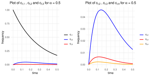
Figure 2. A plot of ${\mathfrak{c}}_{t,i}$ for $i=1,...,4$ for $\alpha=0.5$. The right hand side is a scaled version of the first picture excluding the blocks which contain exactly one element.

Remark 2.2.

Theorem 2.5 can be proved based on its characterisation via transition rates, given in Eqs. (2.6) and (2.7), using general theory [19, 11]. However, in view of our proof of the functional limit theorem, we will work with a representation via Poisson integrals, see Subsection 3.1, which also provides the appropriate coupling for $(\mathbf{C}^{n})_{n\geqslant 0}$ so that the convergence in probability in Theorem 2.8 holds. In fact, using this method, we obtain slightly more; we can show that for all $\varepsilon>0$ and any $T>0$,

$${\mathbb{P}}\Big{(}\sup_{0\leqslant t\leqslant T}|\mathbf{C}^{n}_{t}-{\mathfrak{c}}_{t}|\geqslant\varepsilon\Big{)}=O(n^{\alpha-1})\,\textnormal{ as }n\to\infty.$$

The following theorem is a $L_{2}$ version of the law of large numbers, which plays a pivotal role in our proof of the functional limit theorem below and also seems interesting in its own right.

Theorem 2.7 (Law of large numbers — $L_{2}$-version).

For all $T>0$,

$$\sup_{0\leqslant t\leqslant T}\mathbb{E}\left[\|\mathbf{C}_{t}^{n}-{\mathfrak{c}}_{t}\big{\|}_{2}^{2}\right]=O(n^{\alpha-1}).$$

Note that Theorem 2.7 does not directly imply Theorem 2.5.

Our second main result is a functional limit theorem (FLT) for the fluctuations of $\mathbf{C}^{n}$ around its deterministic limit ${\mathfrak{c}}$.

Theorem 2.8 (Functional Limit Theorem).

For $n\in{\mathbb{N}}_{+}$, set $\sigma_{n}\mathrel{\mathop{:}}=n^{\frac{1-\alpha}{2-\alpha}}$ and $\mathbf{U}_{t}^{n}\mathrel{\mathop{:}}=\sigma_{n}(\mathbf{C}_{t}^{n}-{\mathfrak{c}}_{t})$. Then, there exists a Poisson point process ${\mathcal{N}}$ on $[0,\infty)\times(0,\infty)$ with intensity

$${\,\rm d}t\,u^{\alpha-3}{\,\rm d}u,$$

defined on the same probability space as $\mathbf{C}^{n}$, such that for any $T>0$

$${\mathbb{P}}\Big{(}\sup_{0\leqslant t\leqslant T}|U^{n}_{t,i}-U_{t,i}|\geqslant\varepsilon\Big{)}\to 0\,\textnormal{as }n\to\infty.$$

Here, for all $i=1,\ldots,d$, $\mathbf{U}_{i}=(U_{t,i})_{t\geqslant 0}$ is a generalised Ornstein-Uhlenbeck process satisfying

$${\,\rm d}U_{t,i}=\langle\nabla F_{i}({\mathfrak{c}}_{t}),\mathbf{U}_{t}\rangle{\,\rm d}t+{\,\rm d}M_{t,i},$$

see (2.8) for the definition of $F_{i}$; the driving martingale $\mathbf{M}_{i}$ is defined as

$$M_{t,i}\mathrel{\mathop{:}}=-i\int_{[0,t)\times[0,\infty)}{\mathfrak{c}}_{s,i}u\,\widetilde{\mathcal{N}}({\,\rm d}s{\,\rm d}u),$$

where here and in the following $\widetilde{{\mathcal{N}}}$ denotes the compensation of ${\mathcal{N}}$. Put differently, $U_{i}$ satisfies

$${\,\rm d}U_{t,i}=\langle\nabla F_{i}({\mathfrak{c}}_{t}),\mathbf{U}_{t}\rangle{\,\rm d}t-i{\mathfrak{c}}_{t,i}{\,\rm d}L_{t},$$

where $L$ is a spectrally positive Lévy process with Lévy measure $u^{\alpha-3}{\,\rm d}u$ driven by ${\mathcal{N}}$.

Remark 2.3.

We expect our results to carry over to the more general situation that $\Lambda(\{0\})=\Lambda(\{1\})=0$ and there exists $y_{0}\leqslant 1$ such that

$$\Lambda({\,\rm d}y)=g(y){\,\rm d}y\textnormal{ for, }y\in[0,y_{0}]\quad\textnormal{ and }\quad\lim_{y\to 0+}g(y)y^{1-\alpha}=A,$$ (2.9)

for some $A\in(0,\infty)$ and $\alpha\in(0,1)$; see Assumption (A) in [22]. However, to keep technicalities in check, we restrict ourselves to measures with densities of the form (2.5).

In particular, a result in this spirit was obtained for the Beta coalescent in [22], where it is shown that the fluctuations of the block counting process of the Beta coalescent around its deterministic limit fulfils a functional limit theorem. More precisely, under the assumption in (2.9), they prove that the fluctuations are given by $(2-\alpha)$ stable process of Ornstein-Uhlenbeck type, see Theorem 1.2 in [22]. However, note that in their work they are able to start the coalescent with infinitely many lineages.

3. Proofs

3.1. Integral/Poisson representation

The main device that is used in the proofs of Theorems 2.5, 2.7 and 2.8 is a representation of the normalised block size spectrum $\mathbf{C}^{n}$ in terms of an integral equation with respect to a Poisson measure similar to $N$ (see beginning of Section 2), but augmented by additional information regarding which blocks are affected by each merger. For this, we let $N^{E}$ (the ‘E’ stands for ‘extended’) be a Poisson point process on $[0,\infty)\times[0,1]\times[0,1]^{\mathbb{N}}$ with intensity

$$\mu^{E}({\,\rm d}t,{\,\rm d}u,{\,\rm d}x)\mathrel{\mathop{:}}={\,\rm d}t\frac{\Lambda({\,\rm d}u)}{u^{2}}{\,\rm d}\mathbf{x},$$

where ${\,\rm d}\mathbf{x}$ stands for the uniform distribution on $[0,1]^{\mathbb{N}}$. In other words, $N^{E}$ may be constructed by first constructing the process $N$ as in Eq. (2.1), and then sampling, independently for each atom $(t,u)$, a third component $\mathbf{x}$ as a realisation of a random variable $\mathbf{X}=(X_{1},X_{2},\ldots)$ where $X_{i},i\in{\mathbb{N}}$ are independent random variables, uniformly distributed on $[0,1]$.

In analogy with our earlier habit of referring to atoms $(t,u)$ of $N$ as $u$-mergers, we refer to an atom $(t,u,\mathbf{x})$ of $N^{E}$ as a $(u,\mathbf{x})$-merger. The idea is to index the blocks of $\Pi^{n}$ and their elements in a consistent manner by ${\mathbb{N}}$, such that upon an $(u,\mathbf{x})$-merger, the $i$-th vertex participates in a merger if and only if $x_{i}\leqslant u$.

Let us be a bit more precise. By exchangeability, we can assume without loss of generality that, whenever $\mathbf{C}_{t}^{n}=\mathbf{c}$, say, $\pi=\Pi^{n}_{tn^{\alpha-1}}$ has the following form.

• The $nc_{1}$ singleton blocks of $\pi$ are $\{1\},\{2\},\ldots,\{nc_{1}\}$.

• The $nc_{2}$ blocks of $\pi$ of size $2$ are $\{nc_{1}+1,nc_{1}+2\},\{nc_{1}+3,nc_{1}+4\},\ldots,\{nc_{1}+2nc_{2}-1,nc_{1}+2nc_{2}\}$.

• In general, the $k$-th block of size $i$ is given by $I_{i,k}\mathrel{\mathop{:}}=\{S_{i}+(k-1)i+1,\ldots,S_{i}+ki\}$ with $S_{i}\mathrel{\mathop{:}}=nc_{1}+2nc_{2}+\ldots+(i-1)nc_{i-1}$.

Consequently, for any $1\leqslant i\leqslant d$ and $1\leqslant k\leqslant nc_{i}$,

$$B_{i,k}\mathrel{\mathop{:}}=\big{\{}(u,\mathbf{x})\in[0,1]\times[0,1]^{\mathbb{N}}:\exists j\in I_{i,k}\textnormal{ s.t. }x_{j}\leqslant u\big{\}}$$

is the set of all $(u,\mathbf{x})$ for which the $k$-th block of size $i$ is marked by an $(u,\mathbf{x})$-merger. We also define

$$B_{\geqslant}\mathrel{\mathop{:}}=\big{\{}(u,\mathbf{x})\in[0,1]\times[0,1]^{\mathbb{N}}:\exists\|\mathbf{c}\|n+1\leqslant j\leqslant n\textnormal{ s.t. }x_{j}\leqslant u\big{\}},$$

the set of all $(u,\mathbf{x})$ for which some block with more than $d$ vertices is marked. Note that $B_{j,q}$ and $B_{\geqslant}$ all depend implicitly on $\mathbf{c}$ as well as $n$.

The advantage of this augmented representation is that, having fixed a realisation of $N^{E}$, there is no additional randomness; each $(u,\mathbf{x})$-merger induces a unique (possibly trivial) transition of $\mathbf{C}^{n}$. For $1\leqslant i\leqslant d$, we will write $f_{i}^{n,+}(\mathbf{c},u,\mathbf{x})$ and $f_{i}^{n,-}(\mathbf{c},u,\mathbf{x})$ for the normalised number of blocks of size $i$ that are gained and lost upon an $(u,\mathbf{x})$-merger.

Clearly, every marked block of size $i$ is lost, except when no other vertex outside of that block is coloured.

$$f_{i}^{n,-}(\mathbf{c},u,\mathbf{x})=\frac{1}{n}\sum_{k=1}^{nc_{i}}{\bf 1}_{B_{i,k}}(u,\mathbf{x})\Big{(}1-\prod_{r\in[n]\setminus I_{i,k}}{\bf 1}_{x_{r}>u}\Big{)}.$$ (3.1)

On the other hand, we gain a block of size $i$ whenever, for some $\boldsymbol{\ell}\in{\mathcal{P}}_{2+}(i)$, exactly $\ell_{j}$ blocks of size $j$ are marked, and no other vertex participates

$$f_{i}^{n,+}(\mathbf{c},u,\mathbf{x})=\frac{1}{n}\sum_{\boldsymbol{\ell}\in{\mathcal{P}}_{2+}(i)}{\bf 1}_{B_{\geqslant n}^{c}}(u,\mathbf{x})\prod_{j=1}^{d}\Big{(}\sum_{\begin{subarray}{c}K\subseteq[nc_{j}]\\ |K|=\ell_{j}\end{subarray}}\prod_{q\in K}{\bf 1}_{B_{j,q}}(u,\mathbf{x})\prod_{r\in[nc_{j}]\setminus K}{\bf 1}_{B_{j,r}^{c}}(u,\mathbf{x})\Big{)}.$$ (3.2)

Finally, we also write

$$f_{i}^{n}(\mathbf{c},u,\mathbf{x})\mathrel{\mathop{:}}=f_{i}^{n,+}(\mathbf{c},u,\mathbf{x})-f_{i}^{n,-}(\mathbf{c},u,\mathbf{x}),$$

for the net change in the (normalised) number of blocks of size $i$ upon a $(u,\mathbf{x})$-merger. To account for the time change, we write $N_{n}^{E}$ for the image of $N^{E}$ under the map $(t,u,\mathbf{x})\mapsto(tn^{1-\alpha},u,\mathbf{x})$. Note that by the Poisson mapping theorem (see, for example, Proposition 11.2 in [25]), $N_{n}^{E}$ is a Poisson point process with intensity

$$\mu_{n}^{E}({\,\rm d}t,{\,\rm d}u,{\,\rm d}\mathbf{x})\mathrel{\mathop{:}}=n^{\alpha-1}\mu^{E}({\,\rm d}t,{\,\rm d}u,{\,\rm d}\mathbf{x})=n^{\alpha-1}{\,\rm d}t\frac{\Lambda({\,\rm d}u)}{u^{2}}{\,\rm d}\mathbf{x}.$$

With this, we now have for all $n\in{\mathbb{N}}_{+}$, $t\geqslant 0$ and $1\leqslant i\leqslant d$,

$$C_{t,i}^{n}=\int_{[0,t)\times[0,1]\times[0,1]^{\mathbb{N}}}f_{i}^{n}\big{(}\mathbf{C}_{s}^{n},u,\mathbf{x}\big{)}N_{n}^{E}({\,\rm d}s,{\,\rm d}u,{\,\rm d}\mathbf{x}).$$

By decomposing $N_{n}^{E}$ into the compensated Poisson measure $\widetilde{N}_{n}^{E}$ and its intensity $\mu_{n}^{E}$, we arrive at

$$C_{t,i}^{n}=\delta_{i,1}+\int_{[0,t)}F_{i}^{n}(\mathbf{C}_{s}^{n}){\,\rm d}s+\widehat{M}_{t,i}^{n},$$ (3.3)

where, for all $\mathbf{c}\in E^{n}$,

$$F_{i}^{n}(\mathbf{c})\mathrel{\mathop{:}}=\int_{[0,1]\times[0,1]^{\mathbb{N}}}f_{i}^{n}\big{(}\mathbf{c},u,\mathbf{x}\big{)}\mu_{n}^{E}({\,\rm d}s,{\,\rm d}u,{\,\rm d}\mathbf{x})$$ (3.4)

and

$$\widehat{M}_{t,i}^{n}\mathrel{\mathop{:}}=\int_{[0,t)\times[0,1]\times[0,1]^{\mathbb{N}}}f_{i}^{n}\big{(}\mathbf{C}_{s}^{n},u,\mathbf{x}\big{)}\widetilde{N}_{n}^{E}({\,\rm d}s,{\,\rm d}u,{\,\rm d}\mathbf{x}).$$ (3.5)

We will also let $\widehat{\mathbf{M}}_{t}^{n}\mathrel{\mathop{:}}=(\widehat{M}_{t,1}^{n},\ldots,\widehat{M}_{t,d}^{n})$ and note that $\widehat{\mathbf{M}}^{n}\mathrel{\mathop{:}}=(\widehat{\mathbf{M}}_{t}^{n})_{t\geqslant 0}$ is a martingale with respect to the filtration generated by $N_{n}^{E}$.

3.2. Structure of the proof / Heuristics

Before diving into the computations, we start by outlining the structure of our arguments. In order to prove the law of large numbers, we will show that the martingale part $\widehat{\mathbf{M}}^{n}_{t}$ vanishes as $n\to\infty$. We will also show (see Lemma 3.1), that the limit of $F_{i}^{n}$ in Eq. (3.4) is given by $F_{i}$ in Theorem 2.5. Taking the limit on both sides of Eq. (3.3) and exchanging the limit with the integral, we expect ${\mathfrak{c}}_{t,i}=\lim_{n\to\infty}C_{t,i}^{n}$ to satisfy the integral equation

$${\mathfrak{c}}_{t,i}=\int_{0}^{t}F_{i}({\mathfrak{c}}_{t}){\,\rm d}s$$

or, equivalently, the ordinary differential equation

$$\frac{{\,\rm d}}{{\,\rm d}t}{\mathfrak{c}}_{t,i}=F_{i}({\mathfrak{c}}_{t}).$$

Controlling the $L^{2}$ norm of the martingale part will lead to the $L^{2}$ version of the law of large numbers in Theorem 2.7.

To obtain the functional limit theorem (FLT), we need a finer understanding of the asymptotics of the martingale $\widehat{\mathbf{M}}^{n}$. For that, it is crucial to observe that due to slowing down time by a factor of $n^{\alpha-1}$, we will only see $u$-mergers for very small $u$ and may neglect effects that are of higher order in $u$. In particular, recall that the probability that any given block of size $i$ is lost during an $u$-merger is $iu+O(u^{2})$ (see Eq. (2.3)) and the probability that such a block is gained is of order $u^{2}$ and thus negligible. We therefore expect the net rate of change in the (normalised) number of blocks of size $i$ to be roughly $-iu{\mathfrak{c}}_{t,i}$, which suggests the approximation

$$\widehat{M}_{t,i}^{n}\approx M_{t,i}^{n}\mathrel{\mathop{:}}=-i\int_{[0,t)\times[0,1]}u{\mathfrak{c}}_{s,i}\widetilde{N}_{n}({\,\rm d}s,{\,\rm d}u),$$ (3.6)

where $\widetilde{N}_{n}$ is a compensated Poisson point process on $[0,\infty)\times(0,1)$ with intensity

$$\mu_{n}({\,\rm d}t,{\,\rm d}u)\mathrel{\mathop{:}}=n^{\alpha-1}\mu({\,\rm d}t,{\,\rm d}u)\mathrel{\mathop{:}}=n^{\alpha-1}{\,\rm d}t\frac{\Lambda({\,\rm d}u)}{u^{2}}.$$

Next, we investigate the asymptotics of the integral on the right-hand side of Eq. (3.6) and give a heuristic for the scaling $\sigma_{n}$ in Theorem 2.8. First, note that due to the presence of the factor $n^{\alpha-1}$ in the density $\mu_{n}$, $\mathbf{M}^{n}$ will vanish as $n\to\infty$, hence we need to scale it up by a factor $\sigma_{n}$ to obtain a nontrivial limit. We see that

$$\sigma_{n}M_{t,i}^{n}=-i\int_{[0,t)\times[0,1]}(\sigma_{n}u){\mathfrak{c}}_{s,i}\widetilde{N}_{n}({\,\rm d}s,{\,\rm d}u)=-i\int_{[0,t)\times[0,\sigma_{n}]}u{\mathfrak{c}}_{s,i}\widetilde{N}_{n}^{\ast}({\,\rm d}s,{\,\rm d}u),$$

where $N_{n}^{\ast}$ is the image of $N_{n}$ under the map $(t,u)\mapsto(t,\sigma_{n}u)$, which is by the Poisson mapping theorem (see again [25]) a Poisson point process with intensity

$$n^{\alpha-1}{\,\rm d}t(u/\sigma_{n})^{\alpha-3}(1-u/\sigma_{n})^{\beta-1}{\,\rm d}(u/\sigma_{n})=\sigma_{n}^{2-\alpha}n^{\alpha-1}{\,\rm d}tu^{\alpha-3}(1-u/\sigma_{n})^{\beta-1}{\,\rm d}u,$$

which converges to the intensity of ${\mathcal{N}}$ in Theorem 2.8 upon choosing $\sigma_{n}=n^{(1-\alpha)/(2-\alpha)}$.

3.3. Rigorous argument

To prepare our proof of Theorem 2.5, we first prove that the functions $F_{i}^{n}$ defined in Eq. (3.4) converge uniformly to $F_{i}$ given in Theorem 2.5. In view of later applications in the proof of Theorem 2.8, we need some quantitative control.

Lemma 3.1.

For $1\leqslant i\leqslant d$, we have

$$\sup_{\mathbf{c}\in E^{n}}|F_{i}^{n}(\mathbf{c})-F_{i}(\mathbf{c})|=O(n^{\alpha-1}).$$

Here and in the following, $O(\cdot)$ refers to the limit $n\to\infty$ unless mentioned otherwise. Additionally, $K>0$ will denote some constant which precise value might change from line to line.

Proof.

Recall the definition of $f_{i}^{n,\pm}$ in Eqs. (3.1) as well as (3.2) and define accordingly, mimicking Eq. (3.4),

$$F_{i}^{n,\pm}(\mathbf{c})\mathrel{\mathop{:}}=n^{\alpha-1}\int_{[0,1]\times[0,1]^{\mathbb{N}}}f_{i}^{n,\pm}(\mathbf{c},u,\mathbf{x})\frac{\Lambda({\,\rm d}u)}{u^{2}}{\,\rm d}\mathbf{x}.$$

Let also

$$F_{i}^{+}(\mathbf{c})\mathrel{\mathop{:}}=\sum_{\boldsymbol{\ell}\in{\mathcal{P}}_{2+}(i)}\prod_{j=1}^{d}\frac{(jc_{j})^{\ell_{j}}}{\ell_{j}!}\Gamma(\alpha+|\boldsymbol{\ell}|-2)$$

and

$$F_{i}^{-}(\mathbf{c})\mathrel{\mathop{:}}=\frac{\Gamma(\alpha)}{1-\alpha}ic_{i}.$$

We will separately show that

$$\sup_{\mathbf{c}\in E^{n}}|F_{i}^{n,\pm}(\mathbf{c})-F_{i}^{\pm}(\mathbf{c})|=O(n^{\alpha-1}).$$

We use the definition of $f_{i}^{n,+}$ (see (3.2)) and the fact that ${\bf 1}_{B_{j,q}}$ depends only on $x_{i}$ with $i\in I_{j,q}$, and $I_{j,q}\cap I_{h,r}=\varnothing$ for $j\neq h$, and that ${\bf 1}_{B_{\geqslant}}$ only depends on $[\|\mathbf{c}\|n+1,\ldots,n]$, which is disjoint from all $I_{j,q}$. We get for $i\in[2,d]\cap{\mathbb{N}}$

$$\begin{split}&F_{i}^{n,+}(\mathbf{c})=n^{\alpha-1}\int_{[0,1]\times[0,1]^{\mathbb{N}}}f_{i}^{n,+}(\mathbf{c},u,\mathbf{x})\frac{\Lambda({\,\rm d}u)}{u^{2}}{\,\rm d}\mathbf{x}\\ &\quad=n^{\alpha-2}\sum_{\boldsymbol{\ell}\in{\mathcal{P}}_{2+}(i)}\int_{0}^{1}(1-u)^{n-n\|\mathbf{c}\|}\prod_{j=1}^{d}\left[\binom{nc_{j}}{\ell_{j}}p_{j}(u)^{\ell_{j}}(1-u)^{jnc_{j}-j\ell_{j}}\right]u^{\alpha-3}(1-u)^{\beta-1}{\,\rm d}u\\ &\quad=n^{\alpha-2}\sum_{\boldsymbol{\ell}\in{\mathcal{P}}_{2+}(i)}\binom{n\mathbf{c}}{\boldsymbol{\ell}}\int_{0}^{1}\left[\prod_{j=1}^{d}p_{j}(u)^{\ell_{j}}\right]u^{\alpha-3}(1-u)^{n-\|\boldsymbol{\ell}\|+\beta-1}{\,\rm d}u,\end{split}$$ (3.7)

with $p_{i}(u)$ as in Eq (2.3), where for the last step, we used the notation

$$\binom{n\mathbf{c}}{\boldsymbol{\ell}}\mathrel{\mathop{:}}=\prod_{j=1}^{d}\binom{nc_{j}}{\ell_{j}}.$$

Next, we deal with the $u$-integration. For this, we need to evaluate for all $\boldsymbol{\ell}\in{\mathcal{P}}_{2+}(i)$ the limit as $n\to\infty$ of the integral

$$\int_{0}^{1}P_{\boldsymbol{\ell}}(u)u^{\alpha-3}(1-u)^{n-\|\boldsymbol{\ell}\|+\beta-1}{\,\rm d}u$$

with $P_{\boldsymbol{\ell}}(u)\mathrel{\mathop{:}}=\prod_{j=1}^{d}p_{j}(u)^{\ell_{j}}=u^{|\boldsymbol{\ell}|}\prod_{j=1}^{d}j^{\ell_{j}}+O(u^{|\boldsymbol{\ell}|+1})$, as $u\to 0$. By Lemma 4.1, we have

$$\int_{0}^{1}P_{\boldsymbol{\ell}}(u)u^{\alpha-3}(1-u)^{n-\|\boldsymbol{\ell}\|+\beta-1}{\,\rm d}u=n^{2-\alpha-|\boldsymbol{\ell}|}\prod_{j=1}^{d}j^{\ell_{j}}\Gamma(\alpha-2+|\boldsymbol{\ell}|)+O(n^{1-\alpha-|\boldsymbol{\ell}|}).$$

Inserting this into Eq. (3.7) and noting that

$$\binom{n\mathbf{c}}{\boldsymbol{\ell}}=\frac{n^{|\boldsymbol{\ell}|}}{\boldsymbol{\ell}!}\prod_{j=1}^{d}c_{j}^{\ell_{j}}+O(n^{|\boldsymbol{\ell}|-1}),$$

uniformly in $\mathbf{c}$ with the convention $\boldsymbol{\ell}!=\mathrel{\mathop{:}}\prod_{j=1}^{d}\ell_{j}!$, we see that

$$\begin{split}F_{i}^{n,+}(\mathbf{c})&=\sum_{\boldsymbol{\ell}\in{\mathcal{P}}_{2+}(i)}\binom{n\mathbf{c}}{\boldsymbol{\ell}}\Big{(}n^{-|\boldsymbol{\ell}|}\Gamma(\alpha-2+|\boldsymbol{\ell}|)\prod_{j=1}^{d}j^{\ell_{j}}+O(n^{-|\boldsymbol{\ell}|-1})\Big{)}\\ &\quad=\sum_{\boldsymbol{\ell}\in{\mathcal{P}}_{2+}(i)}\prod_{j=1}^{d}\frac{(jc_{j})^{\ell_{j}}}{\ell_{j}!}\Gamma(\alpha-2+|\boldsymbol{\ell}|)+O(n^{-1})\\ &\quad=F_{i}^{+}(\mathbf{c})+O(n^{-1}),\end{split}$$

where the error term is uniform in $\mathbf{c}$.

Next, we show the convergence of $F_{i}^{n,-}$. Proceeding as before, we have

$$\begin{split}F_{i}^{n,-}(\mathbf{c})&=n^{\alpha-1}\int_{[0,1]\times[0,1]^{\mathbb{N}}}f_{i}^{n,-}(\mathbf{c},u,\mathbf{x})\frac{\Lambda({\,\rm d}u)}{u^{2}}{\,\rm d}\mathbf{x}\\ &=n^{\alpha-1}c_{i}\int_{0}^{1}p_{i}(u)\big{(}1-(1-u)^{n-i}\big{)}u^{\alpha-3}(1-u)^{\beta-1}{\,\rm d}u\\ &=n^{\alpha-1}ic_{i}\int_{0}^{1}u^{\alpha-2}(1-u)^{\beta-1}\big{(}1-(1-u)^{n-i}\big{)}{\,\rm d}u+O(n^{\alpha-1}),\end{split}$$

where we used in the second step that $p_{i}(u)=iu+O(u^{2})$. From Lemma 4.2 we see that

$$\int_{0}^{1}u^{\alpha-2}(1-u)^{\beta-1}\big{(}1-(1-u)^{n-i}\big{)}=n^{1-\alpha}\frac{\Gamma(\alpha)}{1-\alpha}+O(1),$$

which finishes the proof. ∎

Next, we will prove an a-priori estimate for the martingales $\widehat{M}_{i}^{n}$.

Lemma 3.2.

For all $1\leqslant i\leqslant d$ and $T>0$,

$$\mathbb{E}\left[(\widehat{M}_{T,i}^{n})^{2}\right]=O(n^{\alpha-1}).$$

Proof.

We define, decomposing $f_{i}^{n}$ in Eq. (3.5) into $f_{i}^{n,\pm}$,

$$\widehat{M}_{T,i}^{n,\pm}\mathrel{\mathop{:}}=\int_{[0,T)\times[0,1]\times[0,1]^{\mathbb{N}}}f_{i}^{n,\pm}\big{(}\mathbf{C}_{s}^{n},u,\mathbf{x}\big{)}\widetilde{N}_{n}^{E}({\,\rm d}s,{\,\rm d}u,{\,\rm d}\mathbf{x}).$$

By Ito isometry, we have

$$\mathbb{E}\left[(\widehat{M}_{T,i}^{n,+})^{2}\right]=\int_{[0,T)\times[0,1]\times[0,1]^{\mathbb{N}}}f_{i}^{n,+}(\mathbf{C}_{s}^{n},u,\mathbf{x})^{2}\,\mu_{n}({\,\rm d}s,{\,\rm d}u){\,\rm d}\mathbf{x}.$$ (3.8)

To evaluate this note that for $\mathbf{X}\sim\textnormal{unif}([0,1]^{\mathbb{N}})$, $nf_{i}^{n,+}(\mathbf{C}_{s}^{n},u,\mathbf{X})$ conditional on $\mathbf{C}_{s}^{n}$ is a Bernoulli random variable with success probability

$$\sum_{\boldsymbol{\ell}\in{\mathcal{P}}_{2+}(i)}(1-u)^{n-n\|\mathbf{C}^{n}_{s}\|}\prod_{j=1}^{d}\binom{nC^{n}_{s,j}}{\ell_{j}}p_{j}(u)^{\ell_{j}}(1-u)^{j(nC^{n}_{s,j}-\ell_{j})}.$$

Thus, the integral on the right-hand side of Eq. (3.8) evaluates to

$$\begin{split}&\quad n^{\alpha-3}\sum_{\boldsymbol{\ell}\in{\mathcal{P}}_{2+}(i)}\int_{[0,T)\times[0,1]}\binom{n\mathbf{C}^{n}_{s}}{\boldsymbol{\ell}}P_{\boldsymbol{\ell}}(u)u^{\alpha-3}(1-u)^{n-\|\boldsymbol{\ell}\|+\beta-1}{\,\rm d}u{\,\rm d}s\\ &\quad\leqslant K\sum_{\boldsymbol{\ell}\in{\mathcal{P}}_{2+}(i)}n^{\alpha-3+|\boldsymbol{\ell}|}\int_{0}^{1}P_{\boldsymbol{\ell}}(u)u^{\alpha-3}(1-u)^{n-\|\boldsymbol{\ell}\|+\beta-1}{\,\rm d}u,\end{split}$$

with $P_{\boldsymbol{\ell}}(u)=\prod_{j=1}^{d}j^{\ell_{j}}u^{|\boldsymbol{\ell}|}+O(u^{|\boldsymbol{\ell}|+1})$ as $u\to 0$ and some uniform constant $K$. By Lemma 4.1, we have the estimate

$$\int_{0}^{1}P_{\boldsymbol{\ell}}(u)u^{\alpha-3}(1-u)^{n-\|\boldsymbol{\ell}\|+\beta-1}{\,\rm d}u=O(n^{2-\alpha-|\boldsymbol{\ell}|}).$$

We have thus shown that

$$\mathbb{E}\left[(\widehat{M}_{T,i}^{n,+})^{2}\right]=O(n^{-1})=O(n^{\alpha-1}).$$ (3.9)

We now turn to estimating $\mathbb{E}\left[(\widehat{M}_{T,i}^{n,-})^{2}\right]$. Again by Ito isometry,

$$\mathbb{E}\left[(\widehat{M}_{T,i}^{n,-})^{2}\right]=\int_{[0,T)\times[0,1]\times[0,1]^{\mathbb{N}}}f_{i}^{n,-}(\mathbf{C}_{s}^{n},u,\mathbf{x})^{2}\,\mu_{n}({\,\rm d}s,{\,\rm d}u){\,\rm d}\mathbf{x}.$$

Recall the definition of $f_{i}^{n,-}$ in Eq. (3.1). Bounding the number of marked blocks of size $i$ by the number of coloured vertices we see that for $\mathbf{X}\sim\textnormal{unif}([0,1]^{\mathbb{N}})$ and fixed $u\in[0,1]$ and $\mathbf{c}\in E^{n}$, there is $B\sim\textnormal{Binomial}(n,u)$ s.t. $nf_{i}^{n,-}(\mathbf{c},u,\mathbf{X})$ is dominated by $B{\bf 1}_{B\geqslant 2}$ so that we get the bound

$$\mathbb{E}\left[(\widehat{M}_{T,i}^{n,-})^{2}\right]\leqslant Kn^{\alpha-3}\int_{0}^{1}\mathbb{E}\left[B^{2}{\bf 1}_{B\geqslant 2}\right]u^{\alpha-3}(1-u)^{\beta-1}{\,\rm d}u,$$

for some uniform constant $K>0$. A short calculation gives

$$\mathbb{E}\left[B^{2}{\bf 1}_{B\geqslant 2}\right]\leqslant n^{2}u^{2}+nu\big{(}1-(1-u)^{n}\big{)}.$$

Clearly,

$$\int_{0}^{1}u^{\alpha-1}(1-u)^{\beta-1}{\,\rm d}u<\infty,$$

and by Lemma 4.2,

$$\int_{0}^{1}u^{\alpha-2}\big{(}1-(1-u)^{n}\big{)}(1-u)^{\beta-1}=O(n^{1-\alpha}).$$

Altogether, this shows that $\mathbb{E}\left[(\widehat{M}_{T,i}^{n,-})^{2}\right]=O(n^{\alpha-1})$ and together with Eq. (3.9), this concludes the proof. ∎

We are now ready to prove the law of large numbers.

Proof of Theorem 2.5.

Let $\varepsilon>0$ and $i\in\{1,\dots,d\}$, we start from the representation (3.3)

$$C_{t,i}^{n}=\delta_{i,1}+\int_{0}^{t}F_{i}^{n}(\mathbf{C}_{s}^{n}){\,\rm d}s+\widehat{M}_{t,i}^{n}.$$

By definition, ${\mathfrak{c}}$ is the solution of the integral equation

$${\mathfrak{c}}_{t,i}=\delta_{i,1}+\int_{0}^{t}F_{i}({\mathfrak{c}}_{s}){\,\rm d}s.$$

Thus, we have for all $t\in[0,T]$

$$C_{t,i}^{n}-{\mathfrak{c}}_{t,i}=\int_{0}^{t}F_{i}^{n}(\mathbf{C}_{s}^{n})-F_{i}(\mathbf{C}_{s}^{n}){\,\rm d}s+\int_{0}^{t}F_{i}(\mathbf{C}_{s}^{n})-F_{i}({\mathfrak{c}}_{s}){\,\rm d}s+\widehat{M}_{t,i}^{n}.$$

Lemma 3.1 yields a deterministic bound for the first integral.

$$\left|\int_{0}^{t}F_{i}^{n}(\mathbf{C}_{s}^{n})-F_{i}(\mathbf{C}_{s}^{n}){\,\rm d}s\right|\leqslant\int_{0}^{t}|F_{i}^{n}(\mathbf{C}_{s}^{n})-F_{i}(\mathbf{C}_{s}^{n})|{\,\rm d}s\leqslant T\sup_{\mathbf{c}\in E^{n}}|F_{i}^{n}(\mathbf{c})-F_{i}(\mathbf{c})|=O(n^{\alpha-1}).$$

Setting

$$D_{t}^{n}\mathrel{\mathop{:}}=\max_{1\leqslant i\leqslant d}|C_{t,i}^{n}-{\mathfrak{c}}_{t,i}|$$ (3.10)

and noting that $F_{i}$ is smooth implies

$$D_{t}^{n}\leqslant K\int_{0}^{t}D_{s}^{n}{\,\rm d}s+\max_{1\leqslant i\leqslant d}|\widehat{M}_{t,i}^{n}|+O(n^{\alpha-1}).$$

For $\varepsilon^{\prime}>0$, let $A_{n,\varepsilon^{\prime}}$ be the event that

$$\max_{1\leqslant i\leqslant d}\sup_{t\in[0,T]}|\widehat{M}^{n}_{t,i}|\leqslant\varepsilon^{\prime}.$$

By Doob’s inequality and Lemma 3.2,

$$\mathbb{P}\left[A^{c}_{n,\varepsilon^{\prime}}\right]\leqslant{(\varepsilon^{\prime})}^{-2}\sum_{i=1}^{d}\mathbb{E}\left[(\widehat{M}_{T,i}^{n})^{2}\right]=O(n^{\alpha-1}).$$

Moreover, on the event $A_{n,\varepsilon^{\prime}}$ and for sufficiently large $n$ we have

$$D_{t}^{n}\leqslant K\int_{0}^{t}D_{s}^{n}{\,\rm d}s+2\varepsilon^{\prime}$$

and Grönwall’s inequality implies that

$$D_{t}^{n}\leqslant 2\varepsilon^{\prime}(1+T{\rm e}^{T})\leqslant\varepsilon,$$

for sufficiently small $\varepsilon^{\prime}$ and all $t\in[0,T]$. To conclude, we have shown that for all $i\in\{1,\dots,d\}$

$$\mathbb{P}\left[\sup_{t\in[0,T]}|C_{t,i}^{n}-{\mathfrak{c}}_{t,i}|\geqslant\varepsilon\right]=O(n^{\alpha-1}),$$

from which the claim follows by a union bound. ∎

The proof of the $L^{2}$-version follows along similar lines.

Proof of Theorem 2.7.

Using Eq. (3.5) and the definition of $F_{i}^{n}$ in Lemma 3.1, the representation from Eq. (3.3) reads

$$C_{t,i}^{n}=\delta_{i,1}+\int_{0}^{t}F_{i}^{n}(\mathbf{C}_{s}^{n}){\,\rm d}s+\widehat{M}_{t,i}^{n}.$$

Recalling the definition of ${\mathfrak{c}}$, we have for all $t\in[0,T]$

$$C_{t,i}^{n}-{\mathfrak{c}}_{t,i}=\int_{0}^{t}F_{i}^{n}(\mathbf{C}_{s}^{n})-F_{i}(\mathbf{C}_{s}^{n}){\,\rm d}s+\int_{0}^{t}F_{i}(\mathbf{C}_{s}^{n})-F_{i}(\mathbf{C}_{s}){\,\rm d}s+\widehat{M}_{t,i}^{n}.$$

Bounding the first integral with the help of Lemma 3.1 and using the elementary estimate
$(a+b+c)^{2}\leavevmode\nobreak\ \leqslant\leavevmode\nobreak\ 3(a^{2}+b^{2}+c^{2})$, we see that

$$\begin{split}\big{(}C_{t,i}^{n}-{\mathfrak{c}}_{t,i}\big{)}^{2}&\leqslant 3\Big{(}\int_{0}^{t}F_{i}(\mathbf{C}_{s}^{n})-F_{i}(\mathbf{C}_{s}){\,\rm d}s\Big{)}^{2}+3(\widehat{M}_{t,i}^{n})^{2}+O(n^{\alpha-1})\\ &\leqslant 3\int_{0}^{t}\big{(}F_{i}(\mathbf{C}_{s}^{n})-F_{i}(\mathbf{C}_{s})\big{)}^{2}{\,\rm d}s+3(\widehat{M}_{t,i}^{n})^{2}+O(n^{\alpha-1}),\end{split}$$

where the second step is an application of Jensen’s inequality and the error is uniform in $t\in[0,T]$. Next, we take the maximum over all $1\leqslant i\leqslant d$ and the expectation and obtain, using the smoothness of $F_{i}$,

$$\mathbb{E}\left[\max_{1\leqslant i\leqslant d}\big{(}C^{n}_{t,i}-{\mathfrak{c}}_{t,i}\big{)}^{2}\right]\leqslant K\int_{0}^{t}\mathbb{E}\left[\max_{1\leqslant i\leqslant d}\big{(}C^{n}_{s,i}-{\mathfrak{c}}_{s,i}\big{)}^{2}\right]{\,\rm d}s+O(n^{\alpha-1}),$$

where we also used Lemma 3.2. The claim follows from Gronwall’s inequality. ∎

3.4. The functional limit theorem

As a first step towards the proof of the functional limit theorem 2.8, we make the approximation in Eq. (3.6) precise. Recall that $\sigma_{n}=n^{\frac{1-\alpha}{2-\alpha}}$.

Lemma 3.3.

Let $\widehat{\mathbf{M}}^{n}$ be as in Eq. (3.5) and $\mathbf{M}^{n}$ as in Eq. (3.6). Then, for any $T>0$, $\varepsilon>0$ and $i\in\{1,\ldots,d\}$

$$\mathbb{P}\left[\sup_{t\in[0,T]}\sigma_{n}|\widehat{M}_{t,i}^{n}-M_{t,i}^{n}|\geqslant\varepsilon\right]\to 0,\quad\textnormal{as }n\to\infty.$$

Proof.

By Doob’s inequality, it is enough to show that

$$\sigma_{n}^{2}\mathbb{E}\left[\big{(}\widehat{M}_{T,i}^{n}-M_{T,i}^{n}\big{)}^{2}\right]\to 0.$$

With $\widehat{\mathbf{M}}^{n}=\widehat{\mathbf{M}}^{n,+}-\widehat{\mathbf{M}}^{n,-}$ as in the proof of Lemma 3.2 and by the elementary inequality $(a+b)^{2}\leqslant 2a^{2}+2b^{2}$,

$$\mathbb{E}\left[\big{(}\widehat{M}_{T,i}^{n}-M_{T,i}^{n}\big{)}^{2}\right]\leqslant 2\mathbb{E}\left[(\widehat{M}_{T,i}^{n,+})^{2}\right]+2\mathbb{E}\left[\big{(}\widehat{M}_{T,i}^{n,-}+M_{T,i}^{n}\big{)}^{2}\right].$$

We have already shown (see Eq. (3.9)) that $\mathbb{E}\left[(\widehat{M}_{T,i}^{n,+})^{2}\right]=O(n^{-1})=o(\sigma_{n}^{2})$. By Ito isometry,

$$\begin{split}\mathbb{E}\left[\big{(}\widehat{M}_{T,i}^{n,-}+M_{T,i}^{n}\big{)}^{2}\right]&=\int_{[0,T)\times[0,1]\times[0,1]^{\mathbb{N}}}\mathbb{E}\left[\big{(}f_{i}^{n,-}(\mathbf{C}_{s}^{n},u,x)-iu{\mathfrak{c}}_{s,i}\big{)}^{2}\right]\mu_{n}({\,\rm d}s,{\,\rm d}u){\,\rm d}\mathbf{x}\\ &\leqslant 2\int_{[0,T)\times[0,1]\times[0,1]^{\mathbb{N}}}\mathbb{E}\left[\big{(}f_{i}^{n,-}(\mathbf{C}_{s}^{n},u,x)-iuC_{s,i}^{n}\big{)}^{2}\right]\mu_{n}({\,\rm d}s,{\,\rm d}u){\,\rm d}\mathbf{x}\\ &\quad+2\int_{[0,T)\times[0,1]}\mathbb{E}\left[\big{(}iuC_{s,i}^{n}-iu{\mathfrak{c}}_{s,i}\big{)}^{2}\right]\mu_{n}({\,\rm d}s,{\,\rm d}u).\end{split}$$

We can estimate the second integral with the help of Theorem 2.7. For some constant $K>0$,

$$\int_{[0,T)\times[0,1]}\mathbb{E}\left[\big{(}iuC_{s,i}^{n}-iu{\mathfrak{c}}_{s,i}\big{)}^{2}\right]\mu_{n}({\,\rm d}s,{\,\rm d}u) \leqslant Kn^{\alpha-1}\int_{0}^{1}u^{2}n^{\alpha-1}u^{\alpha-3}(1-u)^{\beta-1}{\,\rm d}u$$

$$=O(n^{2\alpha-2})=o(\sigma_{n}^{2}).$$

To estimate the first integral, we proceed similarly as in the proof of Lemma 3.2. For fixed $u\in[0,1]$ and $\mathbf{c}\in E^{n}$, we have

$$\int_{[0,1]^{\mathbb{N}}}\big{(}f_{i}^{n,-}(\mathbf{c},u,\mathbf{x})-iuc_{i}\big{)}^{2}{\,\rm d}\mathbf{x} \leqslant 2\int_{[0,1]^{\mathbb{N}}}\big{(}f_{i}^{n,-}(\mathbf{c},u,\mathbf{x})-p_{i}(u)c_{i}\big{)}^{2}{\,\rm d}x$$

$$\qquad+2\int_{[0,1]^{\mathbb{N}}}\big{(}p_{i}(u)c_{i}-iuc_{i}\big{)}^{2}{\,\rm d}\mathbf{x}.$$

We bound the first integral via the following probabilistic interpretation. Recalling Eq. (3.1), we have for $\mathbf{X}\sim\textnormal{unif}([0,1]^{\mathbb{N}})$ the following equality in distribution.

$$f_{i}^{n,-}(\mathbf{c},u,\mathbf{X})=\frac{1}{n}B\big{(}{\bf 1}_{B\geqslant 2}+B^{\prime}{\bf 1}_{B=1}\big{)},$$

where $B\sim\textnormal{Binomial}\big{(}nc_{i},p_{i}(u)\big{)}$ and $B^{\prime}\sim\textnormal{Ber}\big{(}1-(1-u)^{n-ic_{i}n}\big{)}$ independently of $B$. This is because upon a $(u,\mathbf{X})$-merger, there is a number $B$ of marked blocks of size $i$. These are removed if either $B\geqslant 2$, or if $B=1$ and there is at least one coloured vertex that is not part of a block of size $i$, which happens with probability $\big{(}1-(1-u)^{n-ic_{i}n}\big{)}$. Thus,

$$\int_{[0,1]^{\mathbb{N}}}\big{(}f_{i}^{n,-}(\mathbf{c},u,\mathbf{x})-p_{i}(u)c_{i}\big{)}^{2}{\,\rm d}\mathbf{x}=n^{-2}\mathbb{E}\left[\big{(}B{\bf 1}_{B\geqslant 2}+B^{\prime}{\bf 1}_{B=1}-np_{i}(u)c_{i}\big{)}^{2}\right].$$ (3.11)

To evaluate this further, note that

$$\big{(}B{\bf 1}_{B\geqslant 2}+B^{\prime}{\bf 1}_{B=1}-np_{i}(u)c_{i}\big{)}^{2}=\big{(}B-np_{i}(u)c_{i}\big{)}^{2}-{\bf 1}_{B=1}{\bf 1}_{B^{\prime}=0}\big{[}1-2np_{i}(u)c_{i}\big{]}.$$

Inserting this into Eq. (3.11), we see that

$$\begin{split}&n^{2}\int_{[0,1]^{\mathbb{N}}}\big{(}f_{i}^{n,-}(\mathbf{c},u,\mathbf{x})-iuc_{i}\big{)}^{2}{\,\rm d}\mathbf{x}\\ &\quad=\textnormal{Var}\left[B\right]+\big{(}2np_{i}(u)c_{i}-1\big{)}\mathbb{P}\left[B=1\right]\mathbb{P}\left[B^{\prime}=0\right]\\ &\quad=nc_{i}p_{i}(u)\big{(}1-p_{i}(u)\big{)}+\big{(}2np_{i}(u)c_{i}-1\big{)}\big{(}nc_{i}p_{i}(u)\big{(}1-p_{i}(u)\big{)}^{nc_{i}-1}\big{)}(1-u)^{n-nc_{i}i}\\ &\quad=nc_{i}p_{i}(u)\big{(}1-(1-u)^{n-i}\big{)}-nc_{i}p_{i}(u)^{2}+2n^{2}c_{i}^{2}p_{i}(u)^{2}(1-u)^{n-i}.\end{split}$$

We separately multiply each of the terms in the last line with $n^{\alpha-3}u^{\alpha-3}(1-u)^{\beta-1}$ and integrate with respect to $u$. We get, making use of the fact $p_{i}(u)\leq iu$

$$n^{\alpha-3}nc_{i}\int_{0}^{1}p_{i}(u)\big{(}1-(1-u)^{n-i}\big{)}u^{\alpha-3}(1-u)^{\beta-1}{\,\rm d}u \leqslant n^{\alpha-2}\Big{(}in^{1-\alpha}\frac{\Gamma(\alpha)}{1-\alpha}+O(1)\Big{)}$$

$$=O(n^{-1})=o(\sigma_{n}^{-2}),$$

by Lemma 4.2. By Lemma 4.1, we get

$$n^{\alpha-3}n^{2}c_{i}^{2}\int_{0}^{1}p_{i}(u)^{2}(1-u)^{n-i}u^{\alpha-3}(1-u)^{\beta-1}{\,\rm d}u \leqslant n^{\alpha-1}\big{(}i^{2}n^{-\alpha}\Gamma(\alpha)+O(n^{-\alpha-1})\big{)}$$

$$=O(n^{-1})=o(\sigma_{n}^{-2}).$$

Moreover, the integration of the middle term gives

$$-n^{\alpha-3}n\int_{0}^{1}c_{i}p_{i}(u)^{2}u^{\alpha-3}(1-u)^{\beta-1}{\,\rm d}u \geqslant-n^{\alpha-2}c_{i}i^{2}\int_{0}^{1}u^{\alpha-1}(1-u)^{\beta-1}{\,\rm d}u$$

$$=O(n^{\alpha-2})=o(\sigma_{n}^{-2}).$$

All of these errors are uniform in $\mathbf{c}$, and the proof is thus finished. ∎

Our final ingredient for the proof of Theorem 2.8 is the convergence of $\sigma_{n}M_{t,i}^{n}$ to $M_{t,i}$. In the next lemma we consider an appropriate coupling of the Poisson point processes ${\mathcal{N}}$ and $N_{n}$ for all $n\in{\mathbb{N}}$.

Lemma 3.4.

For any $T>0$, $\varepsilon>0$ and $i\in\{1,\ldots,d\}$, there exists a coupling of ${\mathcal{N}}$ and $(N_{n})_{n\geq 1}$ such that

$$\mathbb{P}\left[\sup_{t\in[0,T]}|\sigma_{n}M_{t,i}^{n}-M_{t,i}|\geqslant\varepsilon\right]\to 0,\quad\textnormal{as }n\to\infty.$$ (3.12)

Proof.

We will give a construction of $(N_{n})_{n\geqslant 1}$ in terms of ${\mathcal{N}}$. The details of this construction will depend on the sign of $\beta-1$. We start with the case $\beta<1$. Given (a realisation of) ${\mathcal{N}}$, we define, for each $n\in{\mathbb{N}}$, a Poisson point process $N_{n}^{\Delta}$ on $[0,\infty]\times[0,\sigma_{n}]$ with intensity

$$\bigg{(}\Big{(}1-\frac{u}{\sigma_{n}}\Big{)}^{\beta-1}-1\bigg{)}u^{\alpha-3}{\bf 1}_{(0,\sigma_{n})}(u){\,\rm d}s{\,\rm d}u=\left|\Big{(}1-\frac{u}{\sigma_{n}}\Big{)}^{\beta-1}-1\right|u^{\alpha-3}{\bf 1}_{(0,\sigma_{n})}(u){\,\rm d}s{\,\rm d}u.$$

Then, we set

$$N_{n}^{\ast}\mathrel{\mathop{:}}={\mathcal{N}}\cap\big{(}[0,\infty)\times[0,\sigma_{n}]\big{)}+N_{n}^{\Delta},$$

where $+$ stands for the superposition of Poisson point processes. We define $N_{n}$ as the image of $N_{n}$ under the map $(t,u)\mapsto(t,u/\sigma_{n})$. By the Poisson mapping theorem, $N_{n}$ indeed has the desired distribution, i.e. it is a Poisson point process on $[0,\infty)\times(0,1)$ with intensity $\mu_{n}({\,\rm d}t,{\,\rm d}u)$.

In the case $\beta\geqslant 1$, we construct $N_{n}^{\Delta}$ by selecting each point $(t,u)\in{\mathcal{N}}\cap\big{(}[0,\infty)\times[0,\sigma_{n}]\big{)}$ with probability

$$1-\Big{(}1-\frac{u}{\sigma_{n}}\Big{)}^{\beta-1}.$$

Then, $N_{n}^{\Delta}$ is again a Poisson point process with intensity

$$\bigg{(}1-\Big{(}1-\frac{u}{\sigma_{n}}\Big{)}^{\beta-1}\bigg{)}u^{\alpha-3}{\bf 1}_{(0,\sigma_{n})}(u){\,\rm d}s{\,\rm d}u=\left|\Big{(}1-\frac{u}{\sigma_{n}}\Big{)}^{\beta-1}-1\right|u^{\alpha-3}{\bf 1}_{(0,\sigma_{n})}(u){\,\rm d}s{\,\rm d}u,$$

and we define $N_{n}^{\ast}\mathrel{\mathop{:}}={\mathcal{N}}\cap\big{(}[0,\infty)\times[0,\sigma_{n}]\big{)}-N_{n}^{\Delta}$, where $-$ denotes the set difference of Poisson point processes. Again $N_{n}$ is the image of $N_{n}^{\ast}$ under $(t,u)\mapsto(t,u/\sigma_{n})$. Also in this case, it is easily checked that $N_{n}$ has the desired distribution.

With ${\mathcal{N}}_{n}^{\prime}\mathrel{\mathop{:}}={\mathcal{N}}\cap\big{(}[0,\infty)\times(\sigma_{n},\infty)\big{)}$, we have in any case the following decomposition

$${\mathcal{N}}=N_{n}^{\ast}+\textnormal{sgn}(\beta-1)N_{n}^{\Delta}+{\mathcal{N}}_{n}^{\prime}.$$

Applying this to the definition of $M_{t,i}$, we get

$$M_{t,i}=M_{t,i}^{\ast,n}+\textnormal{sgn}(\beta-1)M_{t,i}^{\Delta,n}+M_{t,i}^{\prime,n},$$

where

$$M_{t,i}^{\ast,n} \mathrel{\mathop{:}}=-i\int_{[0,t)\times(0,\sigma_{n})}u{\mathfrak{c}}_{s,i}\widetilde{N}_{n}^{\ast,n}({\,\rm d}s,{\,\rm d}u)$$

$$M_{t,i}^{\Delta,n} \mathrel{\mathop{:}}=-i\int_{[0,t)\times(0,\sigma_{n})}u{\mathfrak{c}}_{s,i}\widetilde{N}_{n}^{\Delta}({\,\rm d}s,{\,\rm d}u),$$

$$M_{t,i}^{\prime,n} \mathrel{\mathop{:}}=-i\int_{[0,t)\times[\sigma_{n},\infty)}u{\mathfrak{c}}_{s,i}\widetilde{\mathcal{N}}^{\prime}_{n}({\,\rm d}s,{\,\rm d}u).$$

Because we have defined $N_{n}$ as the image of $N_{n}^{\ast}$ under the map $(t,u)\mapsto(t,u/\sigma_{n})$, we have $\sigma_{n}M_{t,i}^{n}=M_{t,i}^{\ast,n}$. Consequently,

$$\sup_{t\in[0,T]}|\sigma_{n}M_{t,i}^{n}-M_{t,i}|\leqslant\sup_{t\in[0,T]}|M_{t,i}^{\Delta,n}|+\sup_{t\in[0,T]}|M_{t,i}^{\prime,n}|.$$

In order to not overload the notation we are going to drop the superscript $n$ in the remainder of the proof.

To bound the first supremum, we further split $M_{t,i}^{\Delta}=M_{t,i}^{\Delta,<}+M_{t,i}^{\Delta,\geqslant}$ with

$$M_{t,i}^{\Delta,<}\mathrel{\mathop{:}}=-i\int_{[0,t)\times(0,\sigma_{n}^{1/2})}u{\mathfrak{c}}_{s,i}\widetilde{N}_{n}^{\Delta}({\,\rm d}s,{\,\rm d}u)$$

and

$$M_{t,i}^{\Delta,\geqslant}\mathrel{\mathop{:}}=-i\int_{[0,t)\times[\sigma_{n}^{1/2},\sigma_{n})}u{\mathfrak{c}}_{s,i}\widetilde{N}_{n}^{\Delta}({\,\rm d}s,{\,\rm d}u).$$

By Doob’s inequality and Ito isometry, we have

$$\mathbb{P}\left[\sup_{t\in[0,T]}|M_{t,i}^{\Delta,<}|\geqslant\varepsilon/3\right]\leqslant 9\varepsilon^{-2}\mathbb{E}\left[\big{(}M_{T,i}^{\Delta,<}\big{)}^{2}\right]\leqslant 9\varepsilon^{-2}i^{2}T\int_{0}^{\sigma_{n}^{1/2}}u^{\alpha-1}\Big{|}1-\Big{(}1-\frac{u}{\sigma_{n}}\Big{)}^{\beta-1}\Big{|}{\,\rm d}u.$$

As in the proof of Lemma 4.2, we use the mean value theorem to bound

$$\Big{|}1-\big{(}1-x\big{)}^{\beta-1}\Big{|}\leqslant Kx,$$

for some constant $K$ and all $x\in[0,1/2]$, say. Then, for $n$ sufficiently large so that $\sigma_{n}^{1/2}\leqslant\sigma_{n}/2$, we can bound the right-hand side as follows.

$$9\varepsilon^{-2}i^{2}T\int_{0}^{\sigma_{n}^{1/2}}u^{\alpha-1}\Big{|}1-\Big{(}1-\frac{u}{\sigma_{n}}\Big{)}^{\beta-1}\Big{|}{\,\rm d}u\leqslant 9\varepsilon^{-2}i^{2}TK\sigma_{n}^{-1}\int_{0}^{\sigma_{n}^{1/2}}u^{\alpha}{\,\rm d}u=O\big{(}\sigma_{n}^{(\alpha-1)/2}\big{)},$$

which shows that

$$\mathbb{P}\left[\sup_{t\in[0,T]}|M_{t,i}^{\Delta,<}|\geqslant\varepsilon/3\right]=O\big{(}\sigma_{n}^{(\alpha-1)/2}\big{)}.$$ (3.13)

Next, we deal with $M_{t,i}^{\Delta,\geqslant}$. We decompose

$$M_{t,i}^{\Delta,\geqslant}=-i\int_{[0,t)\times[\sigma_{n}^{1/2},\sigma_{n})}u{\mathfrak{c}}_{s,i}N_{n}^{\Delta}({\,\rm d}s,{\,\rm d}u)+i\int_{[0,t)\times[\sigma_{n}^{1/2},\sigma_{n})}u{\mathfrak{c}}_{s,i}\mu_{n}^{\Delta}({\,\rm d}s,{\,\rm d}u).$$

On the event

$$A_{n,T}\mathrel{\mathop{:}}=\big{\{}({\mathcal{N}}_{n}^{\prime}\cup N_{n}^{\Delta})\cap[0,T)\times[\sigma_{n}^{1/2},\infty)\neq\varnothing\big{\}},$$

the first integral vanishes, and after substituting $v=\sigma_{n}u$, the second one is bounded by

$$iT\sigma_{n}^{\alpha-1}\int_{1/2}^{1}v^{\alpha-2}\big{|}1-(1-v)^{\beta-1}\big{|}{\,\rm d}s{\,\rm d}u.$$

This is of order $O(\sigma_{n}^{\alpha-1})$ since

$$\big{|}1-(1-v)^{\beta-1}\big{|}\leqslant 2+2(1-v)^{\beta-1}\quad\textnormal{for all }v\in(1/2,1).$$

We have thus shown that

$$\lim_{n\to\infty}\mathbb{P}\left[\sup_{t\in[0,T]}|M_{t,i}^{\Delta,\geqslant}|\geqslant\varepsilon/3\right]=\lim_{n\to\infty}\mathbb{P}\left[A_{n,T}\right].$$

A straightforward calculation shows that $\mathbb{P}\left[A_{n,T}\right]\to 0$ as $n\to\infty$. Analogously, one can show that

$$\lim_{n\to\infty}\mathbb{P}\left[\sup_{t\in[0,T]}|M_{t,i}^{\prime}|\geqslant\varepsilon/3\right]=\lim_{n\to\infty}\mathbb{P}\left[A_{n,T}\right]=0.$$

Together with Eq. (3.13), we finally obtain

$$\begin{split}&\lim_{n\to\infty}\mathbb{P}\left[\sup_{t\in[0,T]}|\sigma_{n}M_{t,i}^{n}-iM_{t,i}|\geqslant\varepsilon\right]\\ &\quad\leqslant\lim_{n\to\infty}\Bigg{(}\mathbb{P}\left[\sup_{t\in[0,T]}|M_{t,i}^{\prime}|\geqslant\varepsilon/3\right]+\mathbb{P}\left[\sup_{t\in[0,T]}|M_{t,i}^{\Delta,<}|\geqslant\varepsilon/3\right]+\mathbb{P}\left[\sup_{t\in[0,T]}|M_{t,i}^{\Delta,\geqslant}|\geqslant\varepsilon/3\right]\Bigg{)}\\ &\quad=0.\end{split}$$

∎

We need another a-priori estimate for the size of the fluctuations.

Lemma 3.5.

For all $1\leqslant i\leqslant d$ and $\varepsilon,T>0$ we have

$$\lim_{n\to\infty}\mathbb{P}\left[\sup_{t\in[0,T]}\sigma_{n}(C_{t,i}^{n}-{\mathfrak{c}}_{t,i})^{2}\geqslant\varepsilon\right]=0.$$

Proof.

Following the proof of Theorem 2.5 after Eq. (3.10)

$$\sup_{t\in[0,T]}\sigma^{1/2}_{n}D_{t}^{n}\leqslant K\int_{0}^{T}\sigma_{n}^{1/2}D_{s}^{n}{\,\rm d}s+\max_{1\leqslant i\leqslant d}\sigma_{n}^{1/2}|\widehat{M}_{T,i}^{n}|+O(n^{\alpha-1+\frac{1-\alpha}{4-2\alpha}})$$

and thus, for an appropriate $\varepsilon^{\prime}>0$ by Grönwall’s inequality

$$\mathbb{P}\left[\sup_{t\in[0,T]}\sigma_{n}^{1/2}D_{t}^{n}\geqslant\varepsilon\right]\leqslant(\varepsilon^{\prime})^{-2}\max_{1\leqslant i\leqslant d}\sigma_{n}\mathbb{E}\left[(\widehat{M}_{T,i}^{n})^{2}\right]+O(n^{\alpha-1+\frac{1-\alpha}{4-2\alpha}})=O(n^{\alpha-1+\frac{1-\alpha}{2-\alpha}}),$$

which holds for $n$ large enough and the results follows by taking $n\to\infty$. ∎

Now, we just have to put the pieces together.

Proof of Theorem 2.8.

Recall the decomposition from (3.3)

$$C_{t,i}^{n}=\int_{0}^{t}F_{i}^{n}(\mathbf{C}_{s}^{n}){\,\rm d}s+\widehat{M}_{t,i}^{n}$$

and that $U_{t,i}^{n}=\sigma_{n}\big{(}C_{t,i}^{n}-{\mathfrak{c}}_{t,i}\big{)}$. Hence, we have

$$U_{t,i}^{n}=\sigma_{n}\int_{0}^{t}F_{i}^{n}(\mathbf{C}_{s}^{n})-F_{i}({\mathfrak{c}}_{s}){\,\rm d}s+\sigma_{n}\widehat{M}_{t,i}^{n}$$

and therefore, recalling that

$$U_{t,i}=\int_{0}^{t}\langle\nabla F_{i}({\mathfrak{c}}_{s}),\mathbf{U}_{s}\rangle{\,\rm d}s+M_{t,i},$$

we see that

$$\begin{split}U_{t,i}^{n}-U_{t,i}&=\int_{0}^{t}\Big{(}\sigma_{n}\big{(}F_{i}(\mathbf{C}_{s}^{n})-F_{i}({\mathfrak{c}}_{s})\big{)}-\langle\nabla F_{i}({\mathfrak{c}}_{s}),\mathbf{U}_{s}\rangle\Big{)}{\,\rm d}s+\sigma_{n}\int_{0}^{t}F_{i}^{n}(\mathbf{C}_{s}^{n})-F_{i}(\mathbf{C}_{s}^{n}){\,\rm d}s\\ &\quad+\sigma_{n}\widehat{M}_{t,i}^{n}-M_{t,i}\\ &=\int_{0}^{t}\Big{(}\sigma_{n}\big{(}F_{i}(\mathbf{C}_{s}^{n})-F_{i}({\mathfrak{c}}_{s})\big{)}-\langle\nabla F_{i}({\mathfrak{c}}_{s}),\mathbf{U}_{s}\rangle\Big{)}{\,\rm d}s\\ &\quad+\sigma_{n}\widehat{M}_{t,i}^{n}-M_{t,i}+O(n^{\alpha-1+\frac{1-\alpha}{2-\alpha}}),\end{split}$$

where we used Lemma 3.1 in the last step. Because $F_{i}$ is a polynomial, it is straightforward to see that

$$\sigma_{n}\big{(}F_{i}(\mathbf{C}_{s}^{n})-F_{i}({\mathfrak{c}}_{s})\big{)}=\langle\nabla F_{i}({\mathfrak{c}}_{s}),\mathbf{U}_{s}^{n}\rangle+\mathbf{G}_{s},$$

where

$$|\mathbf{G}_{t}|\leqslant K\sigma_{n}\|\mathbf{C}_{t}^{n}-{\mathfrak{c}}_{t}\|_{\infty}^{2},$$

for some uniform constant $K$, where $\|.\|_{\infty}$ denotes the maximum over all $d$ components. Setting ${\mathcal{U}}_{t}^{n}\mathrel{\mathop{:}}=\|\mathbf{U}_{t}^{n}-\mathbf{U}_{t}\|_{\infty}$, we have (because $\mathbf{c}\mapsto DF_{i}(\mathbf{c})$ is bounded) for some (perhaps different) constant $K$ that

$${\mathcal{U}}_{t}^{n}\leqslant K\int_{0}^{t}{\mathcal{U}}_{s}^{n}{\,\rm d}s+\sup_{t,r\in[0,T]}K\Big{(}\|\sigma_{n}\widehat{\mathbf{M}}_{t}^{n}-\mathbf{M}_{t}\|_{\infty}+\sigma_{n}\|\mathbf{C}_{r}^{n}-{\mathfrak{c}}_{r}\|_{\infty}^{2}\Big{)}+O(n^{\alpha-1+\frac{1-\alpha}{2-\alpha}}).$$

By Grönwall’s inequality, we see that for sufficiently large $n$

$$\mathbb{P}\left[\sup_{t\in[0,T]}{\mathcal{U}}_{t}^{n}\geqslant\varepsilon\right]\leqslant\sum_{i=1}^{d}\mathbb{P}\left[\sup_{t,r\in[0,T]}K\Big{(}|\sigma_{n}\widehat{M}_{t,i}^{n}-M_{t,i}|+\sigma_{n}\|\mathbf{C}_{r}^{n}-{\mathfrak{c}}_{r}\|_{\infty}^{2}\Big{)}\geqslant\frac{\varepsilon}{2+2{\rm e}^{KT}}\right].$$

By Lemmas 3.3, 3.4 and 3.5, the right-hand side goes to $0$ as $n\to\infty$. ∎

4. Some auxiliary results

In the next two lemmas, we provide approximation results for certain integrals that appear throughout the manuscript.

Lemma 4.1.

For all $\theta\in{\mathbb{R}}$, $\alpha\in(0,1)$ and all $k\geqslant 2$,

$$\int_{0}^{1}u^{k+\alpha-3}(1-u)^{n+\theta}{\,\rm d}u=n^{2-\alpha-k}\Gamma(k+\alpha-2)+O(n^{1-\alpha-k}).$$

as $n\to\infty$.

Proof.

Since $k\geq 2$, we have $k+\alpha-3\geq-1$, hence by the definition of the Beta-function

$$\int_{0}^{1}u^{k+\alpha-3}(1-u)^{n+\theta}{\,\rm d}u=\frac{\Gamma(k+\alpha-2)\Gamma(n+\theta+1)}{\Gamma(n+\theta+k+\alpha-2)}.$$

We note that by 6.1.47 in [2] it holds

$$\frac{\Gamma(n+\theta+1)}{\Gamma(n+\theta+k+\alpha-2)}(n+\theta)^{k+\alpha-2}=1+O(n^{-1}),$$

and we arrive at

$$\int_{0}^{1}u^{k+\alpha-3}(1-u)^{n+\theta}{\,\rm d}u =\Gamma(k+\alpha-2)(n+\theta)^{2-\alpha-k}(1+O(n^{-1}))$$

$$=\Gamma(k+\alpha-2)n^{2-\alpha-k}(1+O(n^{-1})).$$

∎

Lemma 4.2.

For all $\theta_{1}\in(-1,\infty),\theta_{2}\in{\mathbb{R}}$ and $\alpha\in(0,1)$,

$$\int_{0}^{1}u^{\alpha-2}(1-u)^{\theta_{1}}\big{(}1-(1-u)^{n+\theta_{2}}\big{)}{\,\rm d}u=n^{1-\alpha}\frac{\Gamma(\alpha)}{1-\alpha}+O(1),$$

as $n\to\infty$.

Proof.

We start by decomposing the integral as

$$\int_{0}^{1/2}u^{\alpha-2}(1-u)^{\theta_{1}}\big{(}1-(1-u)^{n+\theta_{2}}\big{)}{\,\rm d}u+\int_{1/2}^{1}u^{\alpha-2}(1-u)^{\theta_{1}}\big{(}1-(1-u)^{n+\theta_{2}}\big{)}{\,\rm d}u.$$ (4.1)

Clearly, since $\big{(}1-(1-u)^{n+\theta_{2}}\big{)}\leqslant 1$ for $n\geqslant-\theta_{2}$, the second integral in (4.1) can be bounded uniformly in $n$. To deal with the first integral in (4.1), we employ the substitution $u\mapsto un$ and obtain

$$\int_{0}^{1/2}u^{\alpha-2}(1-u)^{\theta_{1}}\big{(}1-(1-u)^{n+\theta_{2}}\big{)}{\,\rm d}u=n^{1-\alpha}\int_{0}^{n/2}u^{\alpha-2}\Big{(}1-\frac{u}{n}\Big{)}^{\theta_{1}}\Big{(}1-\Big{(}1-\frac{u}{n}\Big{)}^{n+\theta_{2}}\Big{)}{\,\rm d}u.$$

We split the integral on the right-hand side into three parts

$$\begin{split}&\int_{0}^{n/2}u^{\alpha-2}\Big{(}1-\frac{u}{n}\Big{)}^{\theta_{1}}\Big{(}1-\Big{(}1-\frac{u}{n}\Big{)}^{n+\theta_{2}}\Big{)}{\,\rm d}u\\ &\quad=\int_{0}^{n/2}u^{\alpha-2}\Big{(}1-\frac{u}{n}\Big{)}^{\theta_{1}}(1-{\rm e}^{-u}){\,\rm d}u+\int_{0}^{n/2}u^{\alpha-2}\Big{(}1-\frac{u}{n}\Big{)}^{\theta_{1}}\Big{(}{\rm e}^{-u}-\Big{(}1-\frac{u}{n}\Big{)}^{n}\Big{)}{\,\rm d}u\\ &\quad\quad+\int_{0}^{n/2}u^{\alpha-2}\Big{(}1-\frac{u}{n}\Big{)}^{\theta_{1}+n}\Big{(}1-\Big{(}1-\frac{u}{n}\Big{)}^{\theta_{2}}\Big{)}{\,\rm d}u.\end{split}$$ (4.2)

To proceed, note that the mean-value theorem implies that

$$\left|1-\Big{(}1-\frac{u}{n}\Big{)}^{\theta_{2}}\right|\leqslant K\frac{u}{n}$$ (4.3)

for all $u\in[0,n/2]$ and some constant $K>0$; here and in the following, $K$ will always denote a constant that may change its value from line to line. Thus, the third integral in Eq. (4.2) can be bounded from above by

$$Kn^{-1}\int_{0}^{n/2}u^{\alpha-1}\Big{(}1-\frac{u}{n}\Big{)}^{n}{\,\rm d}u\leqslant Kn^{-1}\int_{0}^{\infty}u^{\alpha-1}{\rm e}^{-u}{\,\rm d}u=O(n^{-1}),$$

again for some constant $K$ (different from the one above). To bound the second integral, we use Lemma 4.3 and see that

$$\int_{0}^{n/2}u^{\alpha-2}\Big{(}1-\frac{u}{n}\Big{)}^{\theta_{1}}\Big{(}{\rm e}^{-u}-\Big{(}1-\frac{u}{n}\Big{)}^{n}\Big{)}{\,\rm d}u\leqslant Kn^{-1}\int_{0}^{\infty}u^{\alpha}{\rm e}^{-u}{\,\rm d}u=O(n^{-1}).$$

We further decompose the first integral in Eq. (4.2) as follows

$$\begin{split}&\int_{0}^{n/2}u^{\alpha-2}\Big{(}1-\frac{u}{n}\Big{)}^{\theta_{1}}(1-{\rm e}^{-u}){\,\rm d}u\\ &\quad=\int_{0}^{\infty}u^{\alpha-2}(1-{\rm e}^{-u}){\,\rm d}u-\int_{n/2}^{\infty}u^{\alpha-2}(1-{\rm e}^{-u}){\,\rm d}u\\ &\quad\quad+\int_{0}^{n/2}u^{\alpha-2}\Big{(}\Big{(}1-\frac{u}{n}\Big{)}^{\theta_{1}}-1\Big{)}(1-{\rm e}^{-u}){\,\rm d}u.\end{split}$$

The first integral is precisely $\Gamma(\alpha)/(1-\alpha)$, as can be seen by an elementary application of integration by parts. Bounding $1-{\rm e}^{-u}$ in the second integral by $1$, we see that it is bounded in absolute value by $n^{\alpha-1}$. For the third integral, we once more apply Eq. (4.3) to see that

$$\int_{0}^{n/2}\left|u^{\alpha-2}\Big{(}\Big{(}1-\frac{u}{n}\Big{)}^{\theta_{1}}-1\Big{)}(1-{\rm e}^{-u})\right|{\,\rm d}u\leqslant Kn^{-1}\int_{0}^{n/2}u^{\alpha-1}{\,\rm d}u=O(n^{\alpha-1}).$$

∎

Lemma 4.3.

Let $n\in\mathbb{N}$, then for all $u\in[0,\frac{n}{2}]$ it holds

$$\left|\Big{(}1-\frac{u}{n}\Big{)}^{n}-{\rm e}^{-u}\right|\leqslant 2n^{-1}u^{2}e^{-u}.$$

Proof.

Note that $\Big{(}1-\frac{u}{n}\Big{)}^{n}\leq e^{-u}$, hence we have

$$0\leq f(u):=e^{-u}-\Big{(}1-\frac{u}{n}\Big{)}^{n}.$$

Then, for all $u\in[0,\frac{n}{2}]$

$$f^{\prime}(u) =\Big{(}1-\frac{u}{n}\Big{)}^{n-1}-e^{-u}=\frac{\left(1-\frac{u}{n}\right)^{n}-e^{-u}\left(1-\frac{u}{n}\right)}{\left(1-\frac{u}{n}\right)}$$

$$\leq 2\left[e^{-u}-e^{-u}\left(1-\frac{u}{n}\right)\right]=2e^{-u}\frac{u}{n}.$$

Finally, noting that $f(0)=0$, by the mean value theorem

$$f(u)\leq u\sup_{0\leq v\leq u}f^{\prime}(v)\leq 2e^{-u}u^{2}n^{-1},$$

which finishes the proof. ∎

Acknowledgements

Frederic Alberti was funded by the Deutsche Forschungsgemeinschaft (DFG, German Research Foundation) — Project-ID 519713930.

Fernando Cordero was funded by the Deutsche Forschungsgemeinschaft (DFG, German Research Foundation) — Project-ID 317210226 — SFB 1283.

References

- Ald [97] D. Aldous. Brownian excursions, critical random graphs and the multiplicative coalescent. Ann. Probab., 25(2):812–854, 1997.
- AS [72] M. Abramowitz and I. A. Stegun. Handbook of mathematical functions with formulas, graphs, and mathematical tables. 10th printing, with corrections. National Bureau of Standards. A Wiley-Interscience Publication. New York etc.: John Wiley & Sons., 1972.
- BBL [10] J. Berestycki, N. Berestycki, and V. Limic. The -coalescent speed of coming down from infinity. Ann. Probab., 38(1), January 2010.
- Ber [09] N. Berestycki. Recent progress in coalescent theory, volume 16 of Ensaios Matemáticos. Sociedade Brasileira de Matemática, Rio de Janeiro, 2009.
- BM [15] N. Broutin and J. F. Marckert. A new encoding of coalescent processes: applications to the additive and multiplicative cases. Probab. Theory Relat. Fields, 166:515–552, 2015.
- BP [98] S. Brin and L. Page. The anatomy of a large-scale hypertextual web search engine. Computer Networks and ISDN Systems, 33:107–117, 1998.
- Bre [14] P. Bressloff. Waves in neural media. Lecture Notes on Mathematical Modelling in the Life Sciences. New York: Springer, 2014.
- Cra [16] H. Crane. Dynamic random networks and their graph limits. Ann. Appl. Probab., 26(2):691–721, 2016.
- DK [99] P. Donnelly and T. G. Kurtz. Particle representations for measure-valued population models. Ann. Probab., 27(1):166–205, 1999.
- Dur [07] R. Durrett. Random graph dynamics. Cambridge Series in Statistical and Probabilistic Mathematics. Cambridge University Press, 2007.
- EK [86] S.N. Ethier and T.G. Kurtz. Markov Processes: Characterization and Convergence. John Wiley & Sons, Inc., 1986.
- ER [59] P. Erdős and A. Rényi. On random graphs. i. Publ. Math. Debrecen, 6:290–297, 1959.
- ER [60] P. Erdős and A. Rényi. On the evolution of random graphs. Magyar Tud. Akad. Mat. Kutató Int. Közl., 5:17–61, 1960.
- Fel [91] S.L. Feld. Why your friends have more friends than you do. American Journal of Sociology, 96(6):1464–1477, 1991.
- FG [04] N. Fournier and J. S. Giet. Convergence of the Marcus-Lushnikov process. Methodol. Comput. Appl., 6(2):219–231, 2004.
- Gri [18] G. Grimmett. Probability on graphs. Random processes on graphs and lattices., volume 8 of IMS Textb. Cambridge: Cambridge University Press, 2nd edition, 2018.
- JKR [23] S.G.G Johnston, A. Kyprianou, and T. Rogers. Multitype -coalescents. Ann. Appl. Probab., 33(6A):4210–4237, 2023.
- KKEP [20] M. Koutrouli, E. Karatzas, D.P. Espino, and G. A. Pavlopoulos. A guide to conquer the biological network era using graph theory. Front. Bioeng. Biotechnol., 8(34), 2020.
- Kur [70] T.G. Kurtz. Solutions of ordinary differential equations as limits of pure jump Markov processes. J. Appl. Probab., 7, 1970.
- Lem [17] S. Lemaire. A multiplicative coalescent with asynchronous multiple mergers. arXiv Preprint, 2017.
- Lim [19] V. Limic. The eternal multiplicative coalescent encoding via excursions of lévy-type processes. Bernoulli, 25(4A):2479–2507, 2019.
- LT [15] V. Limic and A. Talarczyk. Second-order asymptotics for the block counting process in a class of regularly varying -coalescents. Ann. Probab., 43(3):1419–1455, 2015.
- MP [23] L. Miller and H. H. Pitters. Large-scale behaviour and hydrodynamic limit of beta coalescents. Ann. Appl. Probab., 33(1):1–27, 2023.
- Pit [99] J. Pitman. Coalescents with multiple collisions. Ann. Probab., 27(4):1870–1902, 1999.
- Pri [18] N. Privault. Understanding Markov chains. Examples and applications. Springer Undergrad. Math. Ser. Singapore: Springer, 2nd edition, 2018.
- Sag [99] S. Sagitov. The general coalescent with asynchronous merges of ancestral lines. J. Appl. Probab., 36(4):1116–1125, 1999.
- [27] J. Schweinsberg. Coalescents with simultaneous multiple collisions. Electron. J. Probab., 5:1–50, 2000.
- [28] J. Schweinsberg. A necessary and sufficient condition for the -coalescent to come down from the infinity. Electron. Commun. Prob., 5:1–11, 2000.
- vH [16] R. v.d. Hofstad. Random Graphs and Complex Networks. Cambridge Series in Statistical and Probabilistic Mathematics. Cambridge University Press, 1st edition, 2016.
- Wak [16] J. Wakeley. Coalescent Theory: An Introduction. Roberts, 2016.