Stabilization of a twisted modulus on a mirror of rigid Calabi-Yau manifold

Abstract

We study the stabilization of a twisted modulus in Type IIB flux compactifications on a mirror of the rigid Calabi-Yau threefold. By analyzing the effective action of twisted and untwisted moduli, we find that three-form fluxes satisfying the tadpole cancellation conditions lead to supersymmetric AdS vacua. We also investigate swampland conjectures on this non-geometric background.

1 Introduction

It is important to reveal consistency conditions that the four-dimensional (4D) effective theories admit an ultra-violet completion to a consistent theory of quantum gravity (see for a review, e.g., Ref. Palti:2019pca .) In the context of swampland program Vafa:2005ui ; ArkaniHamed:2006dz ; Ooguri:2006in , moduli fields appearing in the 4D effective action of string theory are of particular interest in testing the swampland conjectures. The vacuum expectation values (VEVs) of moduli fields play important roles in determining the vacuum energy of our universe as well as 4D couplings in the low-energy effective action. Type IIB flux compactifications on Calabi-Yau (CY) orientifolds can stabilize all the complex structure moduli and axio-dilaton Giddings:2001yu . The remaining Kähler moduli will be stabilized at 4D Anti-de Sitter (AdS) minima by utilizing non-perturbative and/or perturbative corrections, as proposed in the Kachru-Kallosh-Linde-Trivedi scenario Kachru:2003aw and Large Volume Scenario Balasubramanian:2005zx . However, the validity of de Sitter (dS) vacua uplifted by certain non-perturbative effects and/or an existence of anti D3-brane is still an important open question Gautason:2018gln ; Bena:2018fqc ; Blumenhagen:2019qcg ; Gao:2020xqh .

In this paper, we focus on a different class of CY manifold, the so-called “non-geometric” CY manifold with vanishing Kähler moduli, i.e., $h^{1,1}=0$. This background geometry will allow a rigorous check of swampland conjectures. In particular, we deal with a mirror of a rigid CY manifold. Such a rigid CY manifold with $h^{2,1}=0$ was used in Type IIA flux compactifications, e.g., DeWolfe-Giryavets-Kachru-Taylor (DGKT) model DeWolfe:2005uu . Since the mirror of the rigid CY manifold does not have the Kähler deformations, one can only focus on the dynamics of complex structure moduli in Type IIB side. The stabilization of complex structure on such a background geometry has been studied in Refs. Becker:2006ks ; Becker:2007dn ; Ishiguro:2021csu ; Bardzell:2022jfh ; Becker:2022hse in several moduli space of the complex structure moduli, but the vacuum structure of both the untwisted and twisted moduli is not fully explored. The purpose of this paper is to provide a method to derive the effective action of twisted moduli by utilizing a mirror symmetry technique in the context of Type IIB flux compactifications. With this prescription, we study the flux compactification of complex structure moduli and verify swampland conjectures such as the AdS/moduli scale separation conjecture and species scale distance conjecture. Our numerical analysis shows that three-form fluxes satisfying the tadpole cancellation condition lead to supersymmetric AdS vacua which are consistent with swampland conjectures.

This paper is organized as follows. In Sec. 2, we briefly review Type IIB flux compactifications on the mirror of the rigid CY manifold, following Refs. Candelas:1990pi ; Becker:2006ks ; Becker:2007dn ; Ishiguro:2021csu . By utilizing the special geometry of the underlying manifold, we write down the flux-induced superpotential, i.e., Gukov-Vafa-Witten (GVW) type superpotential Gukov:1999ya , as a function of untwisted and twisted moduli fields. In Sec. 3, we verify swampland conjectures for the VEVs of moduli fields obtained in Sec. 2. Finally, Sec. 4 is devoted to the conclusions.

2 Setup

In this section, we derive the effective action of both untwisted and twisted moduli in Type IIB flux compactifications. In Sec. 2.1, we briefly review the geometric structure of background geometry. In Sec. 2.2, we show the period vector including the contribution of a twisted modulus whose asymptotic expansion is shown in Sec. 2.3. The effective action in the context of Type IIB flux compactifications is discussed in Sec. 2.4.

2.1 Geometry

We begin with the $1^{9}$ Gepner model Gepner:1987qi ; Lutken:1988zj ; Greene:1988ut which is known as to the ${\cal Z}$ manifold with $b_{11}({\cal Z})=36$ and $b_{21}({\cal Z})=36$ Candelas:1985en ; Strominger:1985it . The Landau-Ginzburg potential is described by

$$W=\sum_{k=1}^{9}y_{k}^{3}\,,$$ (2.1)

where $y_{k}$ is regarded as a homogeneous coordinate of $\mathbb{P}_{8}$.

It was known that a mirror of the rigid CY manifold ${\cal Z}$ is described by a quotient of $\mathbb{P}_{8}[3]$ with a certain group $G$, i.e., $\tilde{\cal Z}=\mathbb{P}_{8}[3]/G$. Although this background geometry is a seven-dimensional manifold, one can consider the same cohomology structure of usual CY threefolds Candelas_1993 . Indeed, the Hodge number of $H^{7}(\tilde{\cal Z})=\oplus_{p+q=7}H_{\bar{\partial}}^{p,q}(\tilde{\cal Z})$ is given by $(h^{0,7},h^{1,6},h^{2,5},h^{3,4},h^{4,3},h^{5,2},h^{6,1},h^{7,0})=(0,0,1,\beta,\beta,1,0,0)$ with $\beta$ being 84 for $\mathbb{P}_{8}[3]$. Hence, the middle cohomology ($H^{2,5},H^{3,4},H^{4,3},H^{5,2}$) has the same structure for the Hodge decomposition of $H^{3}$ for CY threefolds. Furthermore, existence of a unique $(5,2)$-form indicates that the complex structure moduli space is described by special geometry, as an analogue of the unique holomorphic three-form of CY threefolds.

In this paper, we focus on a mirror of the rigid CY manifold $\tilde{\cal Z}=\mathbb{P}_{8}[3]/\mathbb{Z}_{3}$ whose defining equation is given by

$$W=\sum_{i,j=1}^{3}x_{ij}^{3}-3\sum_{k=1}^{3}\phi_{k}e_{k}-3\sum_{m,n,p=1}^{3}s_{mnp}f_{mnp}\,,$$ (2.2)

where $e_{i}\simeq x_{i1}x_{i2}x_{i3}$ and $f_{mnp}\simeq x_{1m}x_{2n}x_{3p}$ with $x_{ij}=y_{3i+j-3}$. Here, $\phi_{k}$ and $s_{mnp}$ correspond to untwisted and twisted moduli fields, respectively. Note that when we turn off the twisted moduli, i.e., $s_{mnp}=0$ $\forall m,n,p$, the background geometry is described by three factorizable tori, each which is defined on $\mathbb{P}_{2}[3]$. In this paper, we turn on one of the twisted moduli fields as an illustrative purpose. It corresponds to a generalization of the analysis of Ref. Ishiguro:2021csu which deals with only untwisted moduli. On top of that, we introduce the orientifold action with the tadpole charge 12 Becker:2006ks . Thanks to the symplectic structure of the background geometry, one can introduce background fluxes in the context of Type IIB flux compactifications.

Before going into the detail of flux compactifications, we describe special geometry on a generalized CY manifold ${\cal M}$. Let us consider a symplectic basis $(A^{a},B_{b})$ of $H_{7}({\cal M},\mathbb{Z})$ with $a,b=0,1,...,b_{4,3}+1$. They satisfy the following relations:

$$A^{a}\cap B_{b}=\delta^{a}_{b},\quad B_{b}\cap A^{a}=-\delta^{a}_{b},\quad A^{a}\cap A^{b}=0\quad B_{a}\cap B_{b}=0.$$ (2.3)

The dual cohomology basis $(A^{a},B_{b})$ of $H_{7}({\cal M},\mathbb{Z})$ is defined such that it satisfies

$$\int_{A^{a}}\alpha_{b}=\int_{Y}{\alpha_{b}\wedge\beta^{a}}=\delta^{a}_{b},\quad\int_{B_{a}}\beta^{b}=\int_{Y}{\beta^{b}\wedge\alpha_{a}}=-\delta^{b}_{a}.$$ (2.4)

Then, we introduce the so-called period vector as follows:

$$\Pi\equiv\begin{pmatrix}F_{a}\\ u^{a}\end{pmatrix}\equiv\begin{pmatrix}\int_{B_{a}}\Omega\\ \int_{A^{a}}\Omega\end{pmatrix}.$$ (2.5)

The projective coordinates $u^{a}$ are defined on moduli space by using an integral of the $(5,2)$-form $\Omega$ over the $A^{a}$-cycle, and $F_{a}$ is a function of $u^{a}$ which is also defined by the corresponding integral. Hence, the $(5,2)$-form $\Omega$ is expanded by

$$\Omega=u^{a}\alpha_{a}-F_{a}\beta^{a}.$$ (2.6)

The number of projective coordinates defined this way is $h^{4,3}+1$. However, the coordinates $u^{a}$ are only defined up to a complex rescaling. Taking into account this factor, we consider the quotient:

$$\tau_{\alpha}=\frac{u^{\alpha}}{u^{0}}\qquad\alpha=1,...,h^{4,3},$$ (2.7)

where the index $\alpha$ excludes 0 from the index $a$. By setting $u^{0}=1$, $\tau_{\alpha}$ becomes a set of dynamical fields, namely the complex structure moduli, and this way gives the right number of coordinates to describe the moduli.

2.2 The periods for twisted moduli

In this research, we examine a specific period vector calculated in Ref. Candelas_1993 . Suppose we let only one of the twisted moduli be non-zero, the period vector is given by

$$\Pi\equiv\begin{pmatrix}F_{0}\\ F_{1}\\ F_{2}\\ F_{3}\\ F_{4}\\ u^{0}\\ u^{1}\\ u^{2}\\ u^{3}\\ u^{4}\end{pmatrix}=f\begin{pmatrix}-\varpi_{QQQ}\\ \varpi_{RQQ}\\ \varpi_{QRQ}\\ \varpi_{QQR}\\ c(\omega^{2}\varpi+\omega\hat{\varpi})\\ \varpi_{RRR}\\ \varpi_{QRR}\\ \varpi_{RQR}\\ \varpi_{RRQ}\\ c(\varpi+\hat{\varpi})\end{pmatrix},$$ (2.8)

where $\omega=e^{\frac{2\pi i}{3}},~{}c=\frac{(2\pi)^{6}i}{3^{5/2}}$ and the gauge factor $f=\prod_{i=1}^{3}J^{-\frac{1}{3}}(\phi_{i})\left(\frac{d\phi_{i}}{dJ}\right)^{1/2}$ with $J(\phi_{i})=\frac{\phi_{i}^{3}}{4^{3}}\frac{(\phi_{i}^{3}+8)^{3}}{(\phi_{i}^{3}-1)^{3}}$. Here and in what follows, we define the untwisted moduli $\phi_{i}$ and twisted modulus $\chi$, respectively. Let us introduce

$$\varpi_{IJK}=\sum_{r=0}^{\infty}\frac{(3\chi)^{3r}}{(3r)!}I(\phi_{1},r)J(\phi_{2},r)K(\phi_{3},r),$$ (2.9)

for $I,J,K=\{Q,R\}$, and $Q$ and $R$ are functions depending on $\phi_{i}$ via $Z_{1},Z_{2}$ as

$$\begin{aligned} Q(\phi_{i},r)&=\frac{(2\pi)^{2}}{3}(-Z_{1}(\phi_{i},r)+Z_{2}(\phi_{i},r)),\\ R(\phi_{i},r)&=\frac{(2\pi)^{2}}{3}(-i\sqrt{3})(\omega^{2}Z_{1}(\phi,r)+\omega Z_{2}(\phi,r)),\end{aligned}$$ (2.10)

with

$$\begin{aligned} Z_{1}(\phi_{i},r)&=&\frac{\Gamma(\frac{1}{3})\Gamma(r+\frac{1}{3})}{\Gamma(\frac{2}{3})}\ _{2}F_{1}\left(\frac{1}{3},r+\frac{1}{3};\frac{2}{3};\phi_{i}^{3}\right),\\ Z_{2}(\phi_{i},r)&=\phi_{i}&\frac{\Gamma(\frac{2}{3})\Gamma(r+\frac{2}{3})}{\Gamma(\frac{4}{3})}\ _{2}F_{1}\left(\frac{2}{3},r+\frac{2}{3};\frac{4}{3};\phi_{i}^{3}\right).\end{aligned}$$ (2.11)

The 5- and 10-th components $\varpi,\hat{\varpi}$ in the period vector are given by

$$\begin{aligned} \varpi=\sum_{r=0}^{\infty}\frac{(3\chi)^{3r+1}}{(3r+1)!}Z_{3}\left(\phi_{1},r\right)Z_{3}\left(\phi_{2},r\right)Z_{3}\left(\phi_{3},r\right),\\ \widehat{\varpi}=\sum_{r=0}^{\infty}\frac{(3\chi)^{3r+2}}{(3r+2)!}Z_{4}\left(\phi_{1},r\right)Z_{4}\left(\phi_{2},r\right)Z_{4}\left(\phi_{3},r\right),\end{aligned}$$ (2.12)

with

$$\begin{aligned} Z_{3}(\phi_{i},r)&=Z_{1}\left(\phi_{i},r+\frac{1}{3}\right),\\ Z_{4}(\phi_{i},r)&=Z_{2}\left(\phi_{i},r+\frac{2}{3}\right).\end{aligned}$$ (2.13)

Now we consider the limit $\chi\rightarrow 0$ that a set of eight periods of the ten basis elements reduce to the periods of three torus. In this limit, $\varpi_{IJK}$ is given by

$$\varpi_{IJK} \simeq I(\phi_{1},0)J(\phi_{2},0)K(\phi_{3},0)\qquad\left(I,J,K=\{Q,R\}\right).$$ (2.14)

Also, $\varpi,\hat{\varpi}$ are given by

$$\begin{aligned} \varpi&\simeq 3\chi Z_{3}\left(\phi_{1},0\right)Z_{3}\left(\phi_{2},0\right)Z_{3}\left(\phi_{3},0\right)\\ &=3\chi\prod_{i=1}^{3}Z_{1}\left(\phi_{i},\frac{1}{3}\right),\\ \widehat{\varpi}&\simeq\frac{(3\chi)^{2}}{2}Z_{4}\left(\phi_{1},0\right)Z_{4}\left(\phi_{2},0\right)Z_{4}\left(\phi_{3},0\right)\\ &=\frac{(3\chi)^{2}}{2}\prod_{i=1}^{3}Z_{2}\left(\phi_{i},\frac{2}{3}\right).\end{aligned}$$ (2.15)

The functions of $Q$ and $R$ have important relations for the untwisted complex structure moduli as follows:

$$\tau_{\alpha}=\frac{Q(\phi_{\alpha})}{R(\phi_{\alpha})}\qquad(\alpha=1,2,3),$$ (2.16)

Hence, we obtain a specific period vector that has three moduli $\tau_{i}~{}(i=1,2,3)$ and twisted modulus $\chi$. We arrive at the period vector:

$$\Pi=\begin{pmatrix}-\tau_{1}\tau_{2}\tau_{3}\\ \tau_{2}\tau_{3}\\ \tau_{1}\tau_{3}\\ \tau_{1}\tau_{2}\\ cf(\omega^{2}\varpi+\omega\hat{\varpi})\\ 1\\ \tau_{1}\\ \tau_{2}\\ \tau_{3}\\ cf(\varpi+\hat{\varpi})\end{pmatrix},$$ (2.17)

where $f=\frac{1}{R(\phi_{1})R(\phi_{2})R(\phi_{3})}$.

2.3 Asymptotic approximation of hypergeometric function

In this section, we examine the asymptotic approximation of hypergeometric function which appears in the period vector. The hypergeometric function ${}_{2}F_{1}$ has a following expansion:

$${}_{2}F_{1}(a,a+m;c;z)=\frac{\Gamma(c)}{\Gamma(c-a)\Gamma(a+m)}(-z)^{-a-m}\sum_{n=0}^{\infty}\frac{(a)_{n+m}(a-c+1)_{n+m}}{n!(n+m)!}$$

$$\times z^{-n}[\log(-z)+\psi(1+n)-\psi(a+n+m)-\psi(c-a-n-m)+\psi(1+n+m)]$$

$$+\frac{\Gamma(c)}{\Gamma(a+m)}(-z)^{-a}\sum_{n=0}^{m-1}\frac{(a)_{n}\Gamma(m-n)}{n!\Gamma(c-a-n)}z^{-n},$$ (2.18)

with $|{\rm arg}(-z)|\leq\pi,|z|>1,c-a\notin\mathbb{Z},m\in\mathbb{N}\cup\{0\}$. Here, all functions are understood by their principal values.

To apply this expression of the hypergeometric function into some elements of the period vector, it is notable that $\phi$ and $\tau$ are asymptotically related as follows. From the relation Candelas_1993 :

$$J(\tau)=\frac{\phi^{3}}{4^{3}}\frac{(\phi^{3}+8)^{3}}{(\phi^{3}-1)^{3}}.\qquad\left(J\sim\frac{1}{12^{3}}e^{-2\pi i\tau}\right),$$ (2.19)

$\phi$ and $\tau$ are related as $\phi\sim\frac{1}{3}e^{-\frac{2\pi i\tau}{3}}$. To satisfy this approximation $\phi\sim\frac{1}{3}e^{-\frac{2\pi i\tau}{3}}$, it becomes apparent that at least the following lower bound for $\text{Im}\tau$ is necessary:

$$\text{Im}\tau>\frac{\text{log}729}{2\pi}.$$ (2.20)

Furthermore, $J(\tau)$ can be explicitly described by using $q$-expansion as follows:

$$12^{3}J(\tau)=\frac{1}{q}+744+\mathcal{O}(q)\qquad(q\equiv e^{2\pi i\tau}).$$ (2.21)

Then, similarly to the above, it becomes necessary to impose further lower bounds on $\text{Im}\tau$ to fulfill $J\sim\frac{1}{12^{3}}e^{-2\pi i\tau}$:

$$\text{Im}\tau>\frac{\text{log}744}{2\pi}.$$ (2.22)

Therefore, our analysis to explore flux vacua is valid for the range $\text{Im}\tau\geq 1.1$.

Then, in the large complex structure regime $\phi\sim\frac{1}{3}e^{-\frac{2\pi i\tau}{3}}=\frac{1}{3}e^{\frac{2\pi{\rm Im}\tau}{3}}e^{-\frac{2\pi i{\rm Re}\tau}{3}}\rightarrow\infty$ with ${\rm Arg}\phi=-\frac{2\pi{\real}\tau}{3}(0\leq{\rm Re}\tau<1)$, $Z_{1},Z_{2}$ appearing in the period vector are given by

$$\begin{aligned} Z_{1}(\phi,0)&\sim(-\phi^{3})^{-\frac{1}{3}}\left[\log(-\phi^{3})-2\psi\left(\frac{1}{3}\right)+2\gamma\right],\\ Z_{2}(\phi,0)&\sim(-\phi^{3})^{-\frac{2}{3}}\left[\log(-\phi^{3})-2\psi\left(\frac{2}{3}\right)+2\gamma\right],\\ \end{aligned}$$ (2.23)

where $z=-\phi^{3}$, $\gamma$ is a Euler’s constant and $\psi(x)$ is a polygamma function. It was known in Ref. Candelas_1993 that the background geometry enjoys the $\Pi_{i}SL(2,\mathbb{Z})_{i}$ modular symmetry associated with three untwisted complex structure moduli $\tau_{i}$. For a fundamental domain of ${\rm Re}\,\tau_{i}$, for instance, we restrict ourselves to the region of $0\leq{\rm Re}\,\tau_{i}<1$ because of $|{\rm arg}(-\phi_{i}^{3})|\leq\pi$, but the other region of ${\rm Re}\,\tau_{i}$ is also possible to analyze. Then, the asymptotic expression of function $R$ is derived as follows:

$$\begin{aligned} R(\phi_{i},0)=&-i\frac{(2\pi)^{2}}{\sqrt{3}}\left(\omega^{2}Z_{1}(\phi_{i},0)+\omega Z_{2}(\phi_{i},0)\right)\\ \sim&-i\frac{(2\pi)^{2}}{\sqrt{3}}\frac{1}{\phi_{i}}\left[2\psi\left(\frac{1}{3}\right)-2\psi\left(\frac{2}{3}\right)\right].\end{aligned}$$ (2.24)

Similarly, for the 5-th and 10-th directions of the period vector, we can obtain the explicit expression of $\varpi,\hat{\varpi}$:

$$\begin{aligned} \varpi&\sim 3\chi\prod_{i=1}^{3}\frac{\Gamma\left(\frac{1}{3}\right)}{(1-\phi_{i}^{3})^{1/3}}&&\sim 3\chi\prod_{i=1}^{3}\frac{\Gamma\left(\frac{1}{3}\right)}{(-1)^{1/3}\phi_{i}},\\ \widehat{\varpi}&\sim\frac{(3\chi)^{2}}{2}\prod_{i=1}^{3}\phi_{i}\frac{\Gamma\left(\frac{2}{3}\right)}{(1-\phi_{i}^{3})^{2/3}}&&\sim\frac{(3\chi)^{2}}{2}\prod_{i=1}^{3}\frac{\Gamma\left(\frac{2}{3}\right)}{(-1)^{2/3}\phi_{i}},\end{aligned}$$ (2.25)

where ${}_{2}F_{1}(a,b;b;z)=(1-z)^{-a}$ and $|\phi_{i}|\rightarrow\infty$. Therefore, in the limit $\text{Im}\tau\rightarrow\infty$, the 5- and 10-th components $\Pi_{5},\Pi_{10}$ in the period vector are given by

$$\begin{aligned} \Pi_{5}&=cf(\omega^{2}\varpi+\omega\hat{\varpi})\\ &\sim\frac{1}{24}\left(\psi\left(\frac{1}{3}\right)-\psi\left(\frac{1}{3}\right)\right)^{-3}\left[-3\chi\omega^{2}\Gamma^{3}\left(\frac{1}{3}\right)+\frac{(3\chi)^{2}}{2}\omega\Gamma^{3}\left(\frac{2}{3}\right)\right],\\ \Pi_{10}&=cf(\varpi+\hat{\varpi})\\ &\sim\frac{1}{24}\left(\psi\left(\frac{1}{3}\right)-\psi\left(\frac{1}{3}\right)\right)^{-3}\left[-3\chi\Gamma^{3}\left(\frac{1}{3}\right)+\frac{(3\chi)^{2}}{2}\Gamma^{3}\left(\frac{2}{3}\right)\right].\end{aligned}$$ (2.26)

2.4 Effective action of untwisted and twisted moduli in Type IIB flux compactification

Here, we discuss Type IIB flux compactifications on the mirror of the rigid CY manifold, following Refs. Ishiguro:2021csu ; Becker_2007_run . The three-form fluxes $F_{3}$ and $H_{3}$ are quantized on each cycle which are defined as

$$\begin{aligned} N_{F_{a}}&\equiv\int_{A^{a}}F_{3},&\quad N_{F_{a+5}}&\equiv\int_{B^{a}}F_{3},\\ N_{H_{a}}&\equiv\int_{A^{a}}H_{3},&\quad N_{H_{a+5}}&\equiv\int_{B^{a}}H_{3},\quad(a=0,...,4)\end{aligned}$$ (2.27)

so that $\{N_{F_{0}},...,N_{F_{9}},N_{H_{0}},...,N_{H_{9}}\}$ becomes a set of integers. When these fluxes are turned on three cycles, GVW superpotential in the 4D effective action is provided by Gukov:1999ya

$$W=\int_{\tilde{\cal{Z}}}G_{3}\wedge\Omega,$$ (2.28)

with $G_{3}\equiv F_{3}-SH_{3}$. Here in what follows, the 4D reduced Plank mass is set to be 1, and $S$ is defined by $S\equiv C_{0}+ie^{-\phi}$ with $C_{0}$ and $\phi$ being the Ramond-Ramond 0-form and 4D dilaton, respectively. Then, we can find an explicit form of the superpotential by taking into account Eqs. (2.6), (2.26) and (2.27) as follows:

$$\begin{aligned} W&=(N_{F_{0}}-SN_{H_{0}})\tau_{1}\tau_{2}\tau_{3}\\ &-\left[(N_{F_{1}}-SN_{H_{1}})\tau_{2}\tau_{3}+(N_{F_{2}}-SN_{H_{2}})\tau_{3}\tau_{1}+(N_{F_{3}}-SN_{H_{3}})\tau_{1}\tau_{2}\right]\\ &-(N_{F_{4}}-SN_{H_{4}})\Pi_{5}\\ &+(N_{F_{5}}-SN_{H_{5}})\\ &+\left[(N_{F_{6}}-SN_{H_{6}})\tau_{1}+(N_{F_{7}}-SN_{H_{7}})\tau_{2}+(N_{F_{8}}-SN_{H_{8}})\tau_{3}\right]\\ &+(N_{F_{9}}-SN_{H_{9}})\Pi_{10}.\end{aligned}$$ (2.29)

The Kähler potential in the case of geometric CY threefolds is given by

$$K=K_{\text{ad}}+K_{\text{cs}}+K_{\text{vol}}=-\text{log}(-i(S-\bar{S}))-\text{log}\left(-i\int\Omega\wedge\bar{\Omega}\right)-2\text{log}\mathcal{V},$$ (2.30)

where $\mathcal{V}$ is the volume of CY threefolds. However, in the non-geometric case, the Kähler moduli has no deformation under the orbifolding as discussed in Ref. Becker_2007_run . The contribution of fixed Kähler moduli modifies the axio-dilaton Kähler potential:

$$K_{\text{ad}}+K_{\text{vol}}=-4\text{log}(-i(S-\bar{S})),$$ (2.31)

As regards the Kähler potential of the complex structure moduli, we employ $K_{\text{cs}}$ as the potential including up to the second order of twisted modulus:

$$\begin{aligned} K_{\text{cs}}&=-\text{log}\left(i\prod_{i=1}^{3}(\tau_{i}-\bar{\tau}_{i})-i\left(\Pi_{5}\bar{\Pi}_{10}-\Pi_{10}\bar{\Pi}_{5}\right)\right)\\ &\sim-\text{log}\left(i\prod_{i=1}^{3}(\tau_{i}-\bar{\tau}_{i})\right)+\frac{(2\pi)^{9}\pi^{3}\Gamma^{6}\left(\frac{1}{3}\right)}{3^{5/2}}\frac{|\chi|^{2}}{|R_{1}R_{2}R_{3}|^{2}}\prod_{i=1}^{3}\frac{|1-\phi_{i}^{3}|^{-\frac{2}{3}}}{\text{Im}\tau_{i}}\\ &\sim-\text{log}\left(i\prod_{i=1}^{3}(\tau_{i}-\bar{\tau}_{i})\right)+A|\chi|^{2}\prod_{i=1}^{3}\frac{1}{\text{Im}\tau_{i}}.\end{aligned}$$ (2.32)

Then, by taking into account Eq. (2.24), we can estimate the value of $A$ as follows:

$$A=\left(\frac{(2\pi)^{2}}{\sqrt{3}}\left[2\psi\left(\frac{1}{3}\right)-2\psi\left(\frac{2}{3}\right)\right]\right)^{-6}\frac{(2\pi)^{9}\pi^{3}\Gamma^{6}\left(\frac{1}{3}\right)}{3^{5/2}},$$ (2.33)

As a result, the 4D scalar potential $V$ is defined in terms of $K$ and $W$:

$$V=e^{K}(K^{I\bar{J}}D_{I}WD_{\bar{J}}\bar{W}-3|W|^{2}),$$ (2.34)

where $D_{I}W\equiv W\partial_{I}K+\partial_{I}W$, $K_{I\bar{J}}\equiv\partial_{I}\partial_{\bar{J}}K$ denotes the Kähler metric, and the index $I$ runs the complex structure moduli and the axio-dilaton.

Finally, we discuss the D3-brane charge that appears in the 4D effective action. The $N_{\text{flux}}$ constituted by the 3-form fluxes is defined as follows:

$$\begin{aligned} N_{\text{flux}}&=\int_{\tilde{\cal Z}}H_{3}\wedge F_{3}\\ &=N_{F_{5}}N_{H_{0}}+N_{F_{6}}N_{H_{1}}+N_{F_{7}}N_{H_{2}}+N_{F_{8}}N_{H_{3}}+N_{F_{9}}N_{H_{4}}\\ &\quad-N_{F_{0}}N_{H_{5}}-N_{F_{1}}N_{H_{6}}-N_{F_{2}}N_{H_{7}}-N_{F_{3}}N_{H_{8}}-N_{F_{4}}N_{H_{9}}.\end{aligned}$$ (2.35)

Moreover, $N_{\text{flux}}$ is canceled by the number of D3-branes ($N_{\text{D3}}$) and O3-planes ($N_{\text{O3}}$) according to the tadpole cancellation condition:

$$N_{\text{flux}}+N_{\text{D3}}-\frac{1}{2}N_{\text{O3}}=0.$$ (2.36)

Given that the specific values of O3-planes are determined by orientifold actions in Ref. Becker_2007_nongeo , the maximum value of $N_{\text{flux}}$ is restricted to 12. Hence, the following upper bound exists for $N_{\text{flux}}$:

$$N_{\text{flux}}\leq 12.$$ (2.37)

3 Numerical analysis and swampland conjectures

In Sec. 3.1, we first numerically analyze the effective action. For the obtained SUSY AdS vacua, we next examine the AdS/moduli scale separation conjecture in Sec. 3.2. Finally, the species scale and distance conjecture on this non-geometric background are discussed in Sec. 3.3.

3.1 SUSY AdS/Minkovski vacua with twisted moduli

We numerically analyze the scalar potential by using the superpotential (2.29) and the Kähler potential (2.31) and (2.32). To search for the flux vacua of scalar potential numerically, we utilize the “FindRoot” function in Mathematica. In this research, we examine the flux vacua within the specified range for the three-form flux quanta:

$$-10\leq\{N_{F_{0}},...,N_{F_{9}},N_{H_{0}},...,N_{H_{9}}\}\leq 10.$$ (3.1)

Considering all possible combinations of three-form fluxes within the range of Eq. (3.1), there are approximately $10^{15}$ sets of fluxes in the isotropic case $\tau:=\tau_{1}=\tau_{2}=\tau_{3}$ and $10^{26}$ sets in the anisotropic case. Note that in the isotropic case, we assume the flux relations $N_{F_{1}}=N_{F_{2}}=N_{F_{3}}$, $N_{F_{6}}=N_{F_{7}}=N_{F_{8}}$, $N_{H_{1}}=N_{H_{2}}=N_{H_{3}}$ and $N_{H_{6}}=N_{H_{7}}=N_{H_{8}}$. To simplify our numerical analysis, we randomly generate sets of fluxes within the range of Eq. (3.1).

Here, we will discuss the necessary constraints involved in the random exploration of stable vacua. As discussed in Sec. 2.3, the obtained flux vacua adhere to the constraint $\text{Im}\tau\geq 1.1$. Considering the limit as $\chi\rightarrow 0$ in Eq. (2.15), we discuss the restriction $|\chi|<1$ on the VEVs of the twisted modulus. Moreover, since we consider the effective supergravity action in perturbative string theory, it is necessary to focus on the weak coupling region $\langle\text{Im}S\rangle=g_{\text{s}}^{-1}>1$. Although it seems to be no lower bound for $N_{\rm flux}$, we constrain the range of fluxes using $|N_{\rm flux}|\leq 12$.

	Minkowski ($W=0$)	AdS ($W\neq 0$)
Isotropic Torus with $|N_{\rm flux}|\leq 12$	0 $\quad(10^{5})$	30 $\quad(10^{4})$
Anisotropic Torus with $|N_{\rm flux}|\leq 12$	0 $\quad(10^{3})$	1 $\quad(6.5\times 10^{4})$

Table 1: The numbers of stable vacua, where the number in the parentheses denotes the generated set of three-form fluxes.

In Table 1, we summarize the number of stable vacua for a given set of fluxes. It turns out that in the random search for flux vacua using Eqs. (2.29) (2.31) (2.32), no SUSY Minkowski solutions were found in the isotropic and anisotropic cases, and only SUSY AdS solutions are allowed. For illustrative purposes, we show the benchmark points for supersymmetric AdS vacua in Table 2, where we list the values of the three-form fluxes as well as the D3-brane charge induced by fluxes $N_{\rm flux}$, and the VEVs of moduli fields and the scalar potential. Note that these vacua are classically stable, and we also present the mass squared of the lightest modulus $m^{2}_{\text{light}}$ in the untwisted and twisted sectors.

Properties	Vacuum 1	Vacuum 2	Vacuum3
$N_{F_{0}}$	4	3	-10
$N_{F_{1}}$	-2	-10	8
$N_{F_{4}}$	7	6	9
$N_{F_{5}}$	-6	9	2
$N_{F_{6}}$	-2	-2	9
$N_{F_{9}}$	2	-9	10
$N_{H_{0}}$	0	-9	1
$N_{H_{1}}$	-5	1	6
$N_{H_{4}}$	-2	6	-5
$N_{H_{5}}$	0	9	-8
$N_{H_{6}}$	1	6	0
$N_{H_{9}}$	4	2	3
$\langle\text{Re}S\rangle$	0.420	-0.461	1.15
$\langle\text{Im}S\rangle$	1.66	1.79	5.38
$\langle\text{Re}\tau\rangle$	0.0522	0.435	0.641
$\langle\text{Im}\tau\rangle$	2.35	1.42	3.31
$\langle\text{Re}\chi\rangle$	-0.125	0.182	-0.824
$\langle\text{Im}\chi\rangle$	0.413	0.590	0.438
$\langle V\rangle$	-1.13	-2.32	-0.210
$N_{\text{flux}}$	4	0	7
$m^{2}_{\text{light}}$	1.28	3.87	7.97

Table 2: The explicit values of SUSY AdS vacua in the isotropic case.

3.2 AdS/moduli scale separation conjecture

For the obtained supersymmetric AdS vacua, we will examine the swampland conjecture. In particular, we focus on the overall untwisted moduli, i.e., $\tau=\tau_{1}=\tau_{2}=\tau_{3}$. The AdS/moduli scale separation conjecture posits that in the AdS minimum, the size of the AdS space cannot be separated from the lightest mass of the moduli Gautason:2018gln . In this context, the following relation exists between the size of the AdS and the lightest modulus:

$$m_{\text{light}}R_{\text{AdS}}\leq c,$$ (3.2)

where $c$ is $\mathcal{O}(1)$ constant. The mass of the lightest modulus satisfies $m_{\text{light}}\sim R_{AdS_{5}}$, and $AdS_{5}\times S^{5}$ solution of type IIB superstring upholds this conjecture. Note that the 5-form fluxes are related to the sizes of $R_{\text{AdS}}$ and $R_{S^{5}}$.

In the following, we will discuss the AdS/moduli scale separation conjecture numerically. Here, we employ the following expression as the specific $R_{\text{AdS}}$ in Ref. Ishiguro:2021csu :

$$R_{\text{AdS}}=\sqrt{\frac{(d-1)(d-2)}{|\Lambda_{\text{AdS}}|}}.$$ (3.3)

Using Eq. (3.3) and the numerical values obtained from the random search of flux vacua, we summarize the distribution of $\sqrt{|m_{\text{light}}^{2}R_{\text{AdS}}^{2}|}$ in Fig 1.

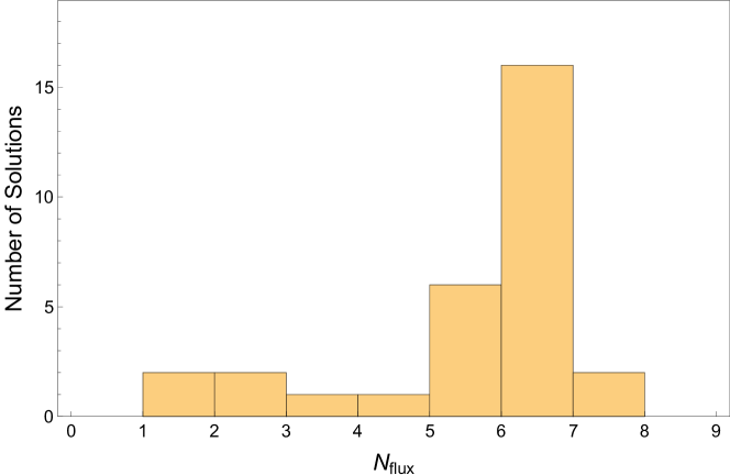
Figure 1: The value of $\sqrt{|m^{2}_{\text{light}}R^{2}_{\text{AdS}}|}$ at SUSY AdS vacua in the isotropic moduli space.

It turns out that this distribution peaks at $\sqrt{|m_{\text{light}}^{2}R_{\text{AdS}}^{2}|}\sim 6$. On the other hand, the results in Ref. Ishiguro:2021csu have peaks at the different value of $\sqrt{|m_{\text{light}}^{2}R_{\text{AdS}}^{2}|}$. According to this result, we can see that the value of $\sqrt{|m_{\text{light}}^{2}R_{\text{AdS}}^{2}|}$ is affected to be larger when moduli stabilization is performed including contributions from twisted sectors.

Figure 2: $\sqrt{|m^{2}_{\text{light}}R^{2}_{\text{AdS}}|}$ v.s. $N_{\rm flux}$ in the isotropic moduli space.

In Fig. 2, we plot the distribution which is the relation between $\sqrt{|m_{\text{light}}^{2}R_{\text{AdS}}^{2}|}$ and $N_{\text{flux}}$. From this results, it can be observed that $\sqrt{|m_{\text{light}}^{2}R_{\text{AdS}}^{2}|}$ has the $N_{\text{flux}}$ dependence. Specifically, small $\sqrt{|m_{\text{light}}^{2}R_{\text{AdS}}^{2}|}$ is less likely to appear in the region of large $N_{\text{flux}}$. In particular, it is found that the solutions with $N_{\text{flux}}=0$ emerge.

3.3 Species scale and distance conjecture

Lastly, we examine the species scale $\Lambda_{s}$ on the non-geometric CY manifold. In the presence of a large number of light particles, the cutoff scale in the 4D EFT is smaller than the Planck scale. This scale is called the species scale Dvali:2007hz ; Dvali:2009ks ; Dvali:2010vm ; Dvali:2012uq . Through the Kaluza-Klein (KK) compactifications, the light degrees of freedom correspond to string and KK modes, and the species scale is given by the string scale for the light string case and the higher-dimensional Planck mass for the light KK case Agmon:2022thq . Indeed, in an infinite-distance limit in the moduli space, it was proposed in Ref. Lee:2019xtm that there are two types of light tower of states in string theory: (i) a tower of light string states corresponding to an emergent string limit at which a charged fundamental string becomes tensionless, and (ii) a tower of light KK states corresponding to a decompactification limit.

In the light string scale, the scale of higher-derivative corrections in the 4D effective action is controlled by the string scale, and the species scale is regarded as a cutoff scale. Then, the species scale is determined by the string scale:

$$\Lambda_{s}^{\rm string}=M_{s}\sim g_{s}M_{\rm Pl}.$$ (3.4)

When we approach the boundary of the moduli space of dilaton, a light tower of states appears in the 4D effective action, as known in the distance conjecture Ooguri:2006in . In a large distance in the moduli space, the typical mass scale in units of 4D reduced Planck mass behaves as

$$m\sim e^{-\lambda\phi},$$ (3.5)

where $\phi$ denotes the canonically normalized modulus, and $\lambda\sim{\cal O}(1)$ in units of $M_{\rm Pl}=1$.

In weakly-coupled perturbative string theory on CY threefolds, the Kähler potential of the 4D axio-dilaton is $K=-\ln(i(\bar{S}-S))$, and the canonical normalization of the 4D dilaton $\phi_{s}=\ln({\rm Im}\,S)/\sqrt{2}$ leads to

$$\Lambda_{s}^{\rm string}\simeq e^{-\frac{\phi_{s}}{\sqrt{2}}}M_{\rm Pl},$$ (3.6)

with $\lambda=1/\sqrt{2}$. Note that in the case of a fundamental string, the tension scales as $T_{\rm string}\sim e^{-\frac{2}{\sqrt{d-2}}\phi_{s}}$ in the $d$-dimensional theory. (For more details, see, e.g., Ref. Etheredge:2022opl .)

In contrast to the geometric CY compactifications, the Kähler potential of the axion dilaton is modified as in (2.31) on the non-geometric background. Thus, the canonical normalization of the 4D dilaton $\phi_{s}=\sqrt{2}\ln({\rm Im}\,S)$ changes the dilaton dependence of the species scale to

$$\Lambda_{s}^{\rm string}\simeq e^{-\frac{\phi_{s}}{2}}M_{\rm Pl},$$ (3.7)

with $\lambda=\frac{1}{2}$. It seems to violate the bound on $\lambda$, i.e., $\lambda\geq\frac{1}{\sqrt{d-2}}$ proposed in Ref. Etheredge:2022opl , but this bound is applicable to the lightest tower of states in an infinite-distance limit of the moduli space. Indeed, the tower of KK mass is lighter than these string states, as will be shown later. On top of that, $\lambda=\frac{1}{2}$ satisfies the bound $\lambda\geq\lambda_{\rm min}=1/\sqrt{(d-1)(d-2)}$ proposed in $d$ dimensions from several theoretical viewpoints Grimm:2018ohb ; Andriot:2020lea ; Gendler:2020dfp ; Lanza:2020qmt ; Bedroya:2020rmd ; Lanza:2021udy ; Calderon-Infante:2023ler .

The KK mass can be extracted from the T-dual Type IIA side. By using the expression of KK mass $m_{\rm KK}$ in Eq. (60) of Ref. Blumenhagen:2019vgj , one can evaluate the lightest KK mass on the mirror of CY manifold:

$$m^{2}_{\rm KK}\simeq\frac{1}{({\rm Im}S)^{2}{\rm Im\tau}_{\rm max}},$$ (3.8)

with ${\rm Im\tau}_{\rm max}\equiv{\rm Max}\{{\rm Im\tau}_{1},{\rm Im\tau}_{2},{\rm Im\tau}_{3}\}$ for the anisotropic case and ${\rm Im\tau}_{\rm max}\equiv{\rm Im\tau}$ for the isotropic case. Here, we assume that the vacuum expectation value of twisted modulus is smaller than that of untwisted modulus, and we show the KK mass associated with the largest untwisted cycle. Hence, the lightest KK mass is smaller than the string scale since the KK mass has an additional suppression factor with respect to the complex structure modulus. After canonically normalizing fields, the lightest KK mass is estimated as

$$m^{2}_{\rm KK}\simeq e^{-\frac{\phi_{s}}{2}-\sqrt{2}\phi_{\tau}},$$ (3.9)

where $\phi_{\tau}=\ln({\rm Im}\,\tau)/\sqrt{2}$ denote the canonically normalized complex structure modulus. Here, we consider the anisotropic case, and $\phi_{\tau}=\sqrt{\frac{3}{2}}\ln({\rm Im}\,\tau)$ in the isotropic case. When there are several infinite towers of light states in a certain infinite-distance limit, $\lambda$ is taken to be the largest one, as discussed in the convex hull swampland distance conjecture Calderon-Infante:2020dhm . For the lightest KK mass (3.9), the maximum value of $\lambda$, i.e., $\lambda=1/\sqrt{2}$, saturates the bound $\lambda\geq 1/\sqrt{d-2}$.

4 Conclusions

In this paper, we have studied the stabilization of both the untwisted and twisted moduli on the mirror of the rigid CY manifold, as an extension of Ref. Ishiguro:2021csu . In this class of background geometry, three-form fluxes can stabilize all the geometric moduli fields due to the lack of Kähler moduli, and it will be a moderate background geometry to verify swampland conjectures.

We present the method to calculate the Type IIB effective action of both untwisted and twisted moduli by utilizing the period vector developed in Ref. Candelas:1990pi . With this prescription, one can write down the flux-induced potential as a function of twisted moduli, as shown in Sec. 2. When we turn on a single twisted modulus, we find that three-form fluxes within the tadpole cancellation condition lead to the stabilization of all of the moduli at supersymmetric AdS vacua. Furthermore, it is possible to realize a small contribution to the tadpole such as $N_{\rm flux}=0$. We restricted ourselves to a single twisted modulus, but it is interesting to explore the vacuum structure of such a mirror of the rigid CY manifold, which is left for future work.

The Kähler potential of the axio-dilaton is different from the usual geometric CY compactifications due to the fixed Kähler moduli. Hence, it is interesting to check the proposed swampland conjectures. In particular, we focused on the AdS/moduli scale separation conjecture and species scale distance conjecture. Our numerical analysis exhibits that the parameter in the AdS/moduli scale separation conjecture is indeed ${\cal O}(1)$ in a similar to the previous analysis Ishiguro:2021csu , and ${\cal O}(1)$ parameter is peaked around a specific value. Furthermore, we examined the species scale for two types of light tower of states in string theory, i.e., a tower of light string states and light KK states. In the case of light string states, the species scale, i.e., the string scale has a novel dependence on the dilaton which leads to the small $\lambda$ in the species scale $\Lambda_{s}\sim e^{-\lambda\phi}$ in contrast to geometric CY compactifications, but it satisfies the bound on the minimum value for $\lambda_{\rm min}=1/\sqrt{(d-1)(d-2)}$. In the case of light KK states, they satisfy the bound on $\lambda$, $\lambda\geq 1/\sqrt{d-2}$, since the lightest tower of states corresponds to KK states in the large complex structure regime of untwisted moduli.

Note added

After finishing this work, we learned of another work Becker:2024ijy where the stabilization of twisted moduli around the Fermat point was studied.

- (1) E. Palti, The Swampland: Introduction and Review, Fortsch. Phys. 67 (2019) 1900037 [1903.06239].
- (2) C. Vafa, The String landscape and the swampland, hep-th/0509212.
- (3) N. Arkani-Hamed, L. Motl, A. Nicolis and C. Vafa, The String landscape, black holes and gravity as the weakest force, JHEP 06 (2007) 060 [hep-th/0601001].
- (4) H. Ooguri and C. Vafa, On the Geometry of the String Landscape and the Swampland, Nucl. Phys. B 766 (2007) 21 [hep-th/0605264].
- (5) S.B. Giddings, S. Kachru and J. Polchinski, Hierarchies from fluxes in string compactifications, Phys. Rev. D 66 (2002) 106006 [hep-th/0105097].
- (6) S. Kachru, R. Kallosh, A.D. Linde and S.P. Trivedi, De Sitter vacua in string theory, Phys. Rev. D 68 (2003) 046005 [hep-th/0301240].
- (7) V. Balasubramanian, P. Berglund, J.P. Conlon and F. Quevedo, Systematics of moduli stabilisation in Calabi-Yau flux compactifications, JHEP 03 (2005) 007 [hep-th/0502058].
- (8) F. Gautason, V. Van Hemelryck and T. Van Riet, The Tension between 10D Supergravity and dS Uplifts, Fortsch. Phys. 67 (2019) 1800091 [1810.08518].
- (9) I. Bena, E. Dudas, M. Graña and S. Lüst, Uplifting Runaways, Fortsch. Phys. 67 (2019) 1800100 [1809.06861].
- (10) R. Blumenhagen, D. Kläwer and L. Schlechter, Swampland Variations on a Theme by KKLT, JHEP 05 (2019) 152 [1902.07724].
- (11) X. Gao, A. Hebecker and D. Junghans, Control issues of KKLT, Fortsch. Phys. 68 (2020) 2000089 [2009.03914].
- (12) O. DeWolfe, A. Giryavets, S. Kachru and W. Taylor, Type IIA moduli stabilization, JHEP 07 (2005) 066 [hep-th/0505160].
- (13) K. Becker, M. Becker, C. Vafa and J. Walcher, Moduli Stabilization in Non-Geometric Backgrounds, Nucl. Phys. B 770 (2007) 1 [hep-th/0611001].
- (14) K. Becker, M. Becker and J. Walcher, Runaway in the Landscape, Phys. Rev. D 76 (2007) 106002 [0706.0514].
- (15) K. Ishiguro and H. Otsuka, Sharpening the boundaries between flux landscape and swampland by tadpole charge, JHEP 12 (2021) 017 [2104.15030].
- (16) J. Bardzell, E. Gonzalo, M. Rajaguru, D. Smith and T. Wrase, Type IIB flux compactifications with h1,1 = 0, JHEP 06 (2022) 166 [2203.15818].
- (17) K. Becker, E. Gonzalo, J. Walcher and T. Wrase, Fluxes, vacua, and tadpoles meet Landau-Ginzburg and Fermat, JHEP 12 (2022) 083 [2210.03706].
- (18) K. Becker, M. Rajaguru, A. Sengupta, J. Walcher and T. Wrase, Stabilizing massless fields with fluxes in Landau-Ginzburg models, 2406.03435.
- (19) P. Candelas and X. de la Ossa, Moduli Space of Calabi-Yau Manifolds, Nucl. Phys. B 355 (1991) 455.
- (20) S. Gukov, C. Vafa and E. Witten, CFT’s from Calabi-Yau four folds, Nucl. Phys. B 584 (2000) 69 [hep-th/9906070].
- (21) D. Gepner, Space-Time Supersymmetry in Compactified String Theory and Superconformal Models, Nucl. Phys. B 296 (1988) 757.
- (22) C.A. Lutken and G.G. Ross, Symmetries and Couplings in Heterotic Superconformal Field Theories, Phys. Lett. B 214 (1988) 357.
- (23) B.R. Greene, C. Vafa and N.P. Warner, Calabi-Yau Manifolds and Renormalization Group Flows, Nucl. Phys. B 324 (1989) 371.
- (24) P. Candelas, G.T. Horowitz, A. Strominger and E. Witten, Vacuum configurations for superstrings, Nucl. Phys. B 258 (1985) 46.
- (25) A. Strominger and E. Witten, New Manifolds for Superstring Compactification, Commun. Math. Phys. 101 (1985) 341.
- (26) P. Candelas, E. Derrick and L. Parkes, Generalized calabi-yau manifolds and the mirror of a rigid manifold, Nuclear Physics B 407 (1993) 115–154.
- (27) K. Becker, M. Becker and J. Walcher, Runaway in the landscape, Physical Review D 76 (2007) .
- (28) K. Becker, M. Becker, C. Vafa and J. Walcher, Moduli stabilization in non-geometric backgrounds, Nuclear Physics B 770 (2007) 1–46.
- (29) G. Dvali, Black Holes and Large N Species Solution to the Hierarchy Problem, Fortsch. Phys. 58 (2010) 528 [0706.2050].
- (30) G. Dvali and D. Lust, Evaporation of Microscopic Black Holes in String Theory and the Bound on Species, Fortsch. Phys. 58 (2010) 505 [0912.3167].
- (31) G. Dvali and C. Gomez, Species and Strings, 1004.3744.
- (32) G. Dvali, C. Gomez and D. Lust, Black Hole Quantum Mechanics in the Presence of Species, Fortsch. Phys. 61 (2013) 768 [1206.2365].
- (33) N.B. Agmon, A. Bedroya, M.J. Kang and C. Vafa, Lectures on the string landscape and the Swampland, 2212.06187.
- (34) S.-J. Lee, W. Lerche and T. Weigand, Emergent strings, duality and weak coupling limits for two-form fields, JHEP 02 (2022) 096 [1904.06344].
- (35) M. Etheredge, B. Heidenreich, S. Kaya, Y. Qiu and T. Rudelius, Sharpening the Distance Conjecture in diverse dimensions, JHEP 12 (2022) 114 [2206.04063].
- (36) T.W. Grimm, E. Palti and I. Valenzuela, Infinite Distances in Field Space and Massless Towers of States, JHEP 08 (2018) 143 [1802.08264].
- (37) D. Andriot, N. Cribiori and D. Erkinger, The web of swampland conjectures and the TCC bound, JHEP 07 (2020) 162 [2004.00030].
- (38) N. Gendler and I. Valenzuela, Merging the weak gravity and distance conjectures using BPS extremal black holes, JHEP 01 (2021) 176 [2004.10768].
- (39) S. Lanza, F. Marchesano, L. Martucci and I. Valenzuela, Swampland Conjectures for Strings and Membranes, JHEP 02 (2021) 006 [2006.15154].
- (40) A. Bedroya, de Sitter Complementarity, TCC, and the Swampland, LHEP 2021 (2021) 187 [2010.09760].
- (41) S. Lanza, F. Marchesano, L. Martucci and I. Valenzuela, The EFT stringy viewpoint on large distances, JHEP 09 (2021) 197 [2104.05726].
- (42) J. Calderón-Infante, A. Castellano, A. Herráez and L.E. Ibáñez, Entropy bounds and the species scale distance conjecture, JHEP 01 (2024) 039 [2306.16450].
- (43) R. Blumenhagen, M. Brinkmann and A. Makridou, Quantum Log-Corrections to Swampland Conjectures, JHEP 02 (2020) 064 [1910.10185].
- (44) J. Calderón-Infante, A.M. Uranga and I. Valenzuela, The Convex Hull Swampland Distance Conjecture and Bounds on Non-geodesics, JHEP 03 (2021) 299 [2012.00034].