S-SOS: Stochastic Sum-Of-Squares for Parametric Polynomial Optimization
Abstract
Global polynomial optimization is an important tool across applied mathematics, with many applications in operations research, engineering, and physical sciences. In various settings, the polynomials depend on external parameters that may be random. We discuss a stochastic sum-of-squares (S-SOS) algorithm based on the sum-of-squares hierarchy that constructs a series of semidefinite programs to jointly find strict lower bounds on the global minimum and extract candidates for parameterized global minimizers. We prove quantitative convergence of the hierarchy as the degree increases and use it to solve unconstrained and constrained polynomial optimization problems parameterized by random variables. By employing -body priors from condensed matter physics to induce sparsity, we can use S-SOS to produce solutions and uncertainty intervals for sensor network localization problems containing up to 40 variables and semidefinite matrix sizes surpassing .
1 Introduction
Many effective nonlinear and nonconvex optimization techniques use local information to identify local minima. But it is often the case that we want to find global optima. Sum-of-squares (SOS) optimization is a powerful and general technique in this setting.
The core idea is as follows: suppose we are given polynomials where each function is on and we seek to determine the minimum value of on the closed set : . Our optimization problem is then to find . An equivalent formulation is to find the largest constant (i.e. the tightest lower bound) that can be subtracted from such that over the set . This reduction converts a polynomial optimization problem over a semialgebraic set to the problem of checking polynomial non-negativity. This problem is NP-hard in general [14], therefore one instead resorts to checking if is a sum-of-squares (SOS) function, e.g. in the unconstrained setting where one seeks to find some polynomials such that . If such a decomposition can be found, then we have an easily checkable certification that , as all sum-of-squares are non-negative but not all non-negative functions are sum-of-squares.
Notably, if we restrict the to have maximum degree , the search for a degree- SOS decomposition of a function can be automated as a semidefinite program (SDP) [28, 21, 24]. Solving this SDP for varying degrees generates the well-known Lasserre (SOS) hierarchy. A given degree corresponds to a particular level of the hierarchy. Solving this SDP produces a lower bound which has been proven to converge to the true global minimum as increases, with finite convergence ( at finite ) for functions with second-order local optimality conditions [30, 5] and asymptotic convergence with milder assumptions thanks to representation theorems for positive polynomials from real algebraic geometry [34, 36]. Further work has elucidated both theoretical implications [34, 21, 20, 23] and useful applications of SOS to disparate fields [33, 29, 10, 30, 5, 2, 32] (see further discussion in Section A.2).
Motivated by the sum-of-squares certification for a lower bound on a function , we generalize to the case where the function to be minimized has additional parameters, i.e. where are variables and are parameters drawn from some probability distribution . We seek a function that is the tightest lower bound to everywhere: with . This setting was originally presented in [22] as a “Joint and Marginal” approach to parametric polynomial optimization. With the view that and seeking to parameterize the minimizers , we are reminded of some of the prior work in polynomial chaos, where a system of stochastic variables is expanded into a deterministic function of those stochastic variables [40, 27].
Contributions and outline. Our primary contributions are a quantitative convergence proof for the Stochastic Sum-of-Squares (S-SOS) hierarchy of semidefinite programs (SDPs), a formulation of a new hierarchy (the cluster basis hierarchy) that uses the structure of a problem to sparsify the SDP, and numerical results on its application to the sensor network localization problem.
In Section 2, we review the S-SOS hierarchy of SDPs [22] and its primal and dual formulations (Section 2.1). We then detail how different hierarchies can be constructed (Section 2.2.1). Finally, in Section 2.3 (complete proofs in Section A.5.2) we specialize to compact and outline the proofs for two theorems on quantitative convergence (the gap between the optimal values of the degree- S-SOS SDP and the “tightest lower-bounding” optimization problem goes as ) of the S-SOS hierarchy for trigonometric polynomials on following the kernel formalism of [13, 5, 38]. The first one applies in the general case and the second one applies to the case where .
In Section 3 we review the hierarchy’s applications in parametric polynomial minimization and uncertainty quantification, focusing on several variants of sensor network localization on . We present numerical results for the accuracy of the extracted solutions that result from S-SOS, comparing to other approaches to parametric polynomial optimization, including a simple Monte Carlo-based method.
2 Stochastic Sum-of-squares (S-SOS)
2.0.1 Notation
Let be the space of polynomials on , where . and , respectively, where and are (not-necessarily compact) subsets of their respective ambient spaces and . A polynomial in can be written as (substituting for a polynomial in ). Let , be a multi-index (size given by context), and be the polynomial coefficients. Let for some denote the subspace of consisting of polynomials of degree , i.e. polynomials where the multi-indices of the monomial terms satisfy . refers to the space of polynomials on that can be expressible as a sum-of-squares in and jointly, and be the same space restricted to polynomials of degree . Additionally, for a matrix denotes that is symmetric positive semidefinite (PSD). Finally, denotes the set of Lebesgue probability measures on . For more details, see Section A.1.
2.1 Formulation of S-SOS hierarchy
We present two formulations of the S-SOS hierarchy that are dual to each other in the sense of Fenchel duality [35, 7]. The primal problem seeks to find the tightest lower-bounding function and the dual problem seeks to find a minimizing probability distribution. Note that the “tightest lower bound” approach is dual to the “minimizing distribution” approach, otherwise known as a “joint and marginal” moment-based approach originally detailed in [22].
2.1.1 Primal S-SOS: The tightest lower-bounding function
Consider a polynomial with equipped with a probability measure . We interpret as our optimization variables and as noise parameters, and seek a lower-bounding function such that for all . In particular, we want the tightest lower bound . Note that even when is polynomial, the tightest lower bound can be non-polynomial. A simple example is the function , which has (Section A.6.1).
For us to select the “best” lower-bounding function, we want to maximize the expectation of the lower-bounding function under while requiring , giving us the following optimization problem over -integrable lower-bounding functions:
| (1) | ||||
| s.t. |
Even if we restricted to be polynomial so that the residual is also polynomial, we would still have a challenging nonconvex optimization problem over non-negative polynomials. In SOS optimization, we take a relaxation and require the residual to be SOS: . Doing the SOS relaxation of the non-negative Equation 1 and restricting , i.e. to polynomials of degree gives us Equation 2, which we call the primal S-SOS degree- SDP:
| (2) | ||||
| s.t. |
where is a basis function containing monomial terms of degree written as a column vector, and a symmetric PSD matrix. Here, represents the dimension of the basis function, which depends on the degree and on the dimensions . For this formulation to find the best degree- approximation to the lower-bounding function, we require to span . Selecting all combinations of standard monomial terms of degree suffices and results in a basis function with size .
2.1.2 Dual S-SOS: A minimizing distribution
The formal dual to Equation 1 (proof of duality in Section A.5.1) seeks to find a “minimizing distribution” , i.e. a probability distribution that places weight on the minimizers of subject to the constraint that the marginal matches :
| (3) | ||||
| s.t. |
where we have written as the space of joint probability distributions on and is the marginal of with respect to , obtained via disintegration.
For the primal, we considered polynomials of degree . We do the same here. The formal dual becomes a tractable SDP, where the objective turns into moment-minimization and the constraints become moment-matching. Following [21, 29], let be the symmetric PSD moment matrix with entries defined as where is the -th element of the basis function . Let be the moment vector of independent moments that completely specifies , e.g. in the case that we use all standard monomials of degree and have , then . We write as the moment matrix that is formed from these independent moments. We have where the multi-index corresponds to the sum of the multi-indices corresponding to the -th entry and the -th entry of .
We write in terms of the monomials , where is the concatenation of the variables from and is a multi-index. Note that every monomial has a corresponding moment : . We then observe that the integral in the objective reduces to a dot product between the coefficients of and the moment vector:
After converting the distribution-matching constraint in (3) into equality constraints on the moments of up to degree , we obtain the following dual S-SOS degree- SDP:
| (4) | ||||
| s.t. | ||||
We write as the set of representing the moment-matching constraints on up to degree-, i.e. we want to set for all multi-indices with . There are multi-indices where only the entries associated with are non-zero, and therefore the number of moment-matching constraints is . Note that the moment matrix is a symmetric PSD matrix and is the dual variable to the primal . Observe also that we require the moments of of degree up to to be bounded. (4) is often a more convenient form than (2), especially when working with additional equality or inequality constraints, as we will see in Section 3. For concrete examples of the primal and dual SDPs with explicit constraints, see Section A.3.
2.2 Variations
In this section, we detail two ways of building a hierarchy, one based on the maximum degree of monomial terms in the basis function (Lasserre) and a novel one based on the maximum number of interactions occurring in the terms of the basis function (cluster basis). To define any SOS hierarchy, we first select a monomial basis. Some examples include the standard monomial basis , trigonometric/Fourier 1-periodic monomial basis ), or others. Using this basis, we write down a basis function which comprises some combinations of monomials. Squared linear combinations of the basis functions then span a SOS space of functions: .
2.2.1 Standard Lasserre hierarchy
In the Lasserre hierarchy, the basis function is composed of all combinations of monomials up to degree and a given level of the hierarchy is set by the maximum degree . The basis function consists of terms with a multi-index and . The degree- SOS function space parameterized by this basis function is that spanned by for PSD , i.e. the functions that can result from squaring any linear combination of degree- polynomials that can be generated from our basis . As we increase the degree , our basis function gets larger and our S-SOS SDP objective values converge to the optimal value of the “tightest lower-bounding” problem Equation 1 [22].
2.2.2 Cluster basis hierarchy
In this section, we propose a cluster basis hierarchy, wherein we utilize possible spatial organization of the problem to sparsify the problem and reduce the size of the SDP that must be solved [41, 8]. The cluster basis is a physically motivated prior often used in statistical and condensed matter physics, where we assume that our degrees of freedom can be arrayed in space, with locally close variables interacting strongly (kept in the model) and globally separated variables interacting weakly (ignored). Moreover, one may also keep only the terms with interactions between a small number of degrees of freedom, such as considering only pairwise or triplet interactions between particles.
In the cluster basis hierarchy, a given level of the hierarchy is defined both by the maximum degree of a variable and the desired body order . Body order denotes the maximum number of interacting variables in a given monomial term, e.g. would have body order 3 and total degree . The basis function consists of terms with a multi-index, (at most interacting variables can occur in a single term), and (each variable can have up to degree . The maximum degree of the basis function is then . If we are to compare from the cluster basis hierarchy with from the Lasserre hierarchy, we find that even when we still have strictly fewer terms, e.g. in the case where we have containing terms of the form but only has degree-4 terms of the . For further details, see discussion in Section A.7.4.
2.3 Convergence of S-SOS
As we increase the degree (either in the Lasserre hierarchy or in the cluster basis hierarchy) we would expect the SDP objective values (Equation 2) to converge to the optimal value and the lower bounding function to converge to the tightest lower bound . In this paper we refer to and interchangeably as strong duality occurs in practice despite being difficult to formally verify (Section A.4). This convergence is a common feature of SOS hierarchies. In this section we show that using polynomial to approximate still allows for asymptotic convergence in as . We further show how this can be improved with other choices of approximating function classes beyond polynomial . We specialize to the particular case of trigonometric polynomials on and compact and prove asymptotic convergence of the degree- S-SOS hierarchy as .
2.3.1 convergence using a polynomial approximation to
We would like to bound the gap between the optimal lower bound and the lower bound resulting from solving the degree- primal S-SOS SDP, i.e.
| (5) |
To that end, we need to understand the regularity of . Without further assumptions, we may assume to be Lipschitz continuous, per Proposition 2.1.
With Equation 5 we may then integrate
where we control in terms of the degree . If we can drive as then we are done.
Proposition 2.1 (Theorem 2.1 in [9]).
Let be polynomial. Then is Lipschitz continuous.
Theorem 2.1 (Asymptotic convergence of S-SOS).
Let be a trigonometric polynomial of degree , the optimal lower bound as a function of , and any probability measure on compact . Let refer to the degree of the basis in both terms and the degree of the lower-bounding polynomial , i.e. is the full basis function of terms with and only has terms with .
Let be the solution to the following S-SOS SDP (c.f. Equation 2) with a spanning basis of trigonometric monomials with degree :
Then there is a constant depending only on such that the following holds:
where denotes the average value of the function over , i.e. and denotes the norm of the Fourier coefficients. Thus we have asymptotic convergence of the S-SOS SDP hierarchy to the optimal value of Equation 1 as we send .
Proof.
The following is an outline of the proof. For complete details, including the full theorem and proof, please see Section A.5.2.
We define a trigonometric polynomial (t.p.) of degree that approximates the lower-bounding function such that . The error integral breaks apart into two terms, one bounding the approximation error between and , and the other bounding the error between the approximate lower-bounding t.p. and the SOS lower-bounding t.p. .
We then follow the proofs of [13, 5, 38] wherein we define an invertible linear operator that constructs a SOS function out of a non-negative function, and show that such an operator exists for sufficiently large . The core modification is to the operator which is defined as an integral operator over two kernels , i.e.
∎
2.3.2 convergence using a piecewise-constant approximation to
Prior work [5] achieves convergence for the regular SOS hierarchy without further assumptions. In the previous section, we could only achieve due to the need to first approximate the tightest lower-bounding function with a polynomial approximation, which converges at a slower rate. To accelerate the convergence rate, we want to control the regularity of . We can achieve by approximating the pointwise instead of using a smooth parameterized polynomial. By constructing a domain decomposition of and finding a SOS approximation in for each domain, we can stitch these together to build a piecewise-constant approximation to the lower-bounding function .
In the one-dimensional case (full proof in Section A.5.2) we achieve the following:
Proposition 2.2.
Let be a compact interval and be a trigonometric polynomial of degree . Let be equi-distant grid points in and the number of such points. Denote by the best SOS approximation of degree of and define
Then we have for some constant depending only on :
3 Numerical experiments
We present two numerical studies of S-SOS demonstrating its use in applications. The first study (Section 3.1) numerically tests how the optimal values of the SDP Equation 2 converge to of the original primal Equation 1 as we increase the degree. The second study (Section 3.2) evaluates the performance of S-SOS for solution extraction and uncertainty quantification in various sensor network localization problems.
3.1 Simple quadratic SOS function
As a simple illustration of S-SOS, we test it on the SOS function
| (6) |
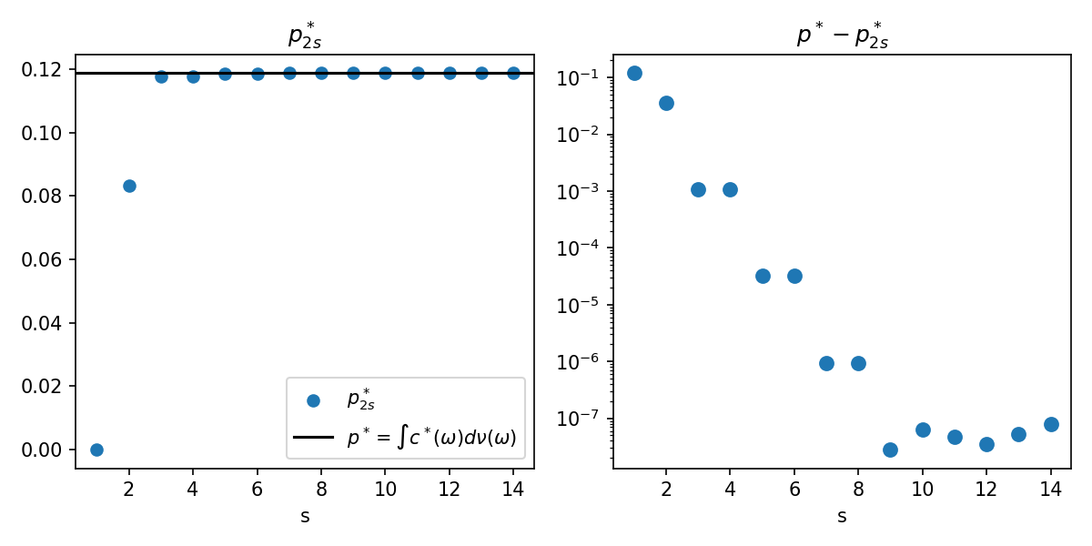
with . The lower bound can be computed analytically as . Assuming , we get that the objective value for the “tightest lower-bounding” primal problem Equation 1 is . For further details, see Section A.6.
We are interested in studying the quantitative convergence of the S-SOS hierarchy numerically. The idea is to solve the primal (dual) degree- SDP to find the tightest polynomial lower bound (the minimizing probability distribution) for varying degrees . As gets larger, the basis function gets larger and the objective value of the SDP Equation 2 should converge to the theoretical optimal value .
In Figure 1 we see very good agreement between and with exponential convergence as increases. This is much faster than the rate we found in Section 2.3.1, but agrees with the exponential convergence results from [5] achieved with local optimality assumptions. Due to the simplicity of (6), it’s not surprising that we see much faster convergence. In fact, for most typical functions, we might expect convergence much faster than the worst-case rate. The tapering-off of the convergence rate is likely attributed to the numerical tolerance used in our solver (CVXPY/MOSEK), as we observed that increasing the tolerance shifts the best-achieved gap higher.
3.2 Sensor network localization
Sensor network localization (SNL) is a common testbed for global optimization and SDP solvers due to the high sensitivity and ill-conditioning of the problem. In SNL, one seeks to recover the positions of sensors positioned in given a set of noisy observations of pairwise distances between the sensors [29, 39]. To have a unique global minimum and remove symmetries, sensor-anchor distance observations are often added, where several sensors are anchored at known locations in the space. This can improve the conditioning of the problem, making it “easier” in some sense.
3.2.1 Definitions
We define a SNL problem instance with as the ground-truth positions for sensors, as the ground-truth positions for anchors, as the set of observed sensor-sensor distances and as the set of observed sensor-anchor distances, both of which depend on some sensing radius .
Writing as the unknown positions of the -th sensor and the -th anchor, we can write the potential function to be minimized as a polynomial:
| (7) |
The observed sensor-sensor and sensor-anchor distances can be perturbed arbitrarily, but in this paper we focus on linear uniform noise, i.e. for a subset of observed distances we have with . Other noise types may be explored, including those including outliers, which may be a better fit for robust methods (Section A.7.2).
Equation 7 contains soft penalty terms for sensor-sensor terms and sensor-anchor terms. We can see that this is a degree-4 polynomial in the standard monomial basis elements, and a global minimum of this function is achieved at (where the distances have not been perturbed by any noise). In general for non-zero (measuring distances under noise perturbations) we expect the function minimum to be , as there may not exist a configuration of sensors that is consistent with the observed noisy distances.
We can also support equality constraints in our solution, in particular hard equality constraints on the positions of certain sensors relative to known anchors. This corresponds to removing all sensor-anchor soft penalty terms from the function and instead selecting sensors at random to exactly fix in known positions via equality constraints in the SDP. The SDP is still large but the effective number of variable sensors has been reduced to .
A given SNL problem type is specified by a spatial dimension , sensors, anchors, a sensing radius , a noise type (linear), and anchor type (soft penalty or hard equality). Once these are specified, we generate a random problem instance by sampling . The potential for a given instance is formed (either with sensor-anchor terms or not, with terms kept based on some sensing radius , and noise variables appropriately added).
The number of anchors is chosen to be as few as possible so as to still enable exact localization, i.e. anchors for a SNL problem in spatial dimensions. The SDPs are formulated with the help of SymPy [26] and solved using CVXPY [11, 1] and Mosek [4] on a server with two Intel Xeon 6130 Gold processors (32 physical cores total) and 256GB of RAM. For an expanded discussion and further details, see Section A.7.
3.2.2 Evaluation metrics
The accuracy of the recovered solution is of primary interest, i.e. our primary evaluation metric should be the distance between our extracted sensor positions and the ground-truth sensor positions , i.e. . Because the S-SOS hierarchy recovers estimates of the sensor positions along with uncertainty estimates , we would like to measure the distance between our ground-truth positions to our estimated distribution . The Mahalanobis distance (Equation 8) is a modified distance metric that accounts for the uncertainty [25]. We use this as our primary metric for sensor recovery accuracy.
| (8) |
As our baseline method, for each problem instance we apply a basic Monte Carlo method detailed in Algorithm 1 (Section A.7.3) where we sample , use a local optimization solver to find , and use this to estimate . Note that though this non-SOS method achieves some estimate of the dual SDP objective , it is not guaranteed to be a lower bound.
3.2.3 Results
Recovery accuracy. In Table 1 we see a comparison of the S-SOS method and the MCPO baseline. Each row corresponds to one SNL problem type, i.e. we fix the physical dimension , the number of anchors , and select the sensing radius and the noise scale . We then generate random instances of each problem type, corresponding to a random realization of the ground-truth sensor and anchor configurations , producing a that we then solve the SDP for (in the case of S-SOS) or do pointwise optimizations for (in the case of MCPO). Each method outputs estimates for the sensor positions and uncertainty around it as a , which we then compute for (see Equation 8), treating each dimension as independent of each other (i.e. as a flat vector). Each instance solve gives us one observation of or each method, and we report the median and the values over the instances we generate.
| Parameters | Basis comparison | M-distance () | ||||||||
| S-SOS | MCPO | |||||||||
| 1 | 0.5 | 0.3 | 0 | 1 | 10 | 78 | 78 | 1x | ||
| 1 | 1.0 | 0.3 | 0 | 1 | 10 | 78 | 78 | 1x | ||
| 1 | 1.5 | 0.3 | 0 | 1 | 10 | 78 | 78 | 1x | ||
| 1 | 1.5 | 0.3 | 2 | 1 | 10 | 78 | 78 | 1x | ||
| 1 | 1.5 | 0.3 | 4 | 1 | 10 | 78 | 78 | 1x | ||
| 1 | 1.5 | 0.3 | 6 | 1 | 10 | 78 | 78 | 1x | ||
| 1 | 1.5 | 0.3 | 8 | 1 | 10 | 78 | 78 | 1x | ||
| 2 | 1.5 | 0.1 | 0 | 9 | 9 | 406 | 163 | 2.5x | ||
| 2 | 1.5 | 0.1 | 0 | 9 | 15 | 820 | 317 | 2.6x | ||
4 Discussion
In this paper, we discuss the stochastic sum-of-squares (S-SOS) method to solve global polynomial optimization in the presence of noise, prove two asymptotic convergence results for polynomial and compact , and demonstrate its application to parametric polynomial minimization and uncertainty quantification along with a new cluster basis hierarchy that enables S-SOS to scale to larger problems. In our experiments, we specialized to sensor network localization and low-dimensional uniform random noise with small . However, it is relatively straightforward to extend this method to support other noise types (such as Gaussian random variates without compact support, which we do in Section A.6.4) and support higher-dimensional noise with .
Scaling this method to larger problems is an open problem for all SOS-type methods. In this paper, we take the approach of sparsification, by making the cluster basis assumption to build up a block-sparse . We anticipate that methods that leverage sparsity or other structure in will be promising avenues of research, as well as approximate solving methods that avoid the explicit materialization of the matrices . For example, we assume that the ground-truth polynomial possesses the block-sparse structure because our SDP explicitly requires the polynomial to exactly decompose into some lower-bounding and SOS . Relaxing this exact-decomposition assumption and generalizing beyond polynomial may require novel approaches and would be an exciting area for future work.
References
- Agrawal et al. [2018] Akshay Agrawal, Robin Verschueren, Steven Diamond, and Stephen Boyd. A rewriting system for convex optimization problems. Journal of Control and Decision, 5(1):42–60, 2018.
- Ahmadi and Majumdar [2019] Amir Ali Ahmadi and Anirudha Majumdar. DSOS and SDSOS Optimization: More Tractable Alternatives to Sum of Squares and Semidefinite Optimization. SIAM Journal on Applied Algebra and Geometry, 3(2):193–230, January 2019. ISSN 2470-6566. doi: 10.1137/18M118935X. URL https://epubs.siam.org/doi/10.1137/18M118935X.
- Ambrosio et al. [2005] Luigi Ambrosio, Nicola Gigli, and Savare. Gradient Flows in Metric Spaces and in the Space of Probability Measures. Birkhäuser, second edition, 2005.
- ApS [2023] MOSEK ApS. The MOSEK optimization toolbox for Python manual. Version 10.0., 2023. URL https://docs.mosek.com/10.0.44/pythonapi/index.html.
- Bach and Rudi [2023] Francis Bach and Alessandro Rudi. Exponential convergence of sum-of-squares hierarchies for trigonometric polynomials, April 2023. URL http://arxiv.org/abs/2211.04889. arXiv:2211.04889 [math].
- Bertsimas et al. [2011] Dimitris Bertsimas, Dan Andrei Iancu, and Pablo A. Parrilo. A Hierarchy of Near-Optimal Policies for Multistage Adaptive Optimization. IEEE Transactions on Automatic Control, 56(12):2809–2824, December 2011. ISSN 0018-9286. doi: 10.1109/TAC.2011.2162878. URL http://ieeexplore.ieee.org/document/5986692/.
- Boyd and Vandenberghe [2004] Stephen Boyd and Lieven Vandenberghe. Convex Optimization. Cambridge University Press, 1 edition, March 2004. ISBN 978-0-521-83378-3 978-0-511-80444-1. doi: 10.1017/CBO9780511804441. URL https://www.cambridge.org/core/product/identifier/9780511804441/type/book.
- Chen et al. [2023] Yian Chen, Yuehaw Khoo, and Lek-Heng Lim. Convex Relaxation for Fokker-Planck, June 2023. URL http://arxiv.org/abs/2306.03292. arXiv:2306.03292 [cs, math].
- Clarke [1975] Frank H. Clarke. Generalized gradients and applications. Transactions of the American Mathematical Society, 205:247–262, 1975. URL https://api.semanticscholar.org/CorpusID:120174258.
- de Klerk [2008] Etienne de Klerk. The complexity of optimizing over a simplex, hypercube or sphere: a short survey. Central European Journal of Operations Research, 16(2):111–125, June 2008. ISSN 1613-9178. doi: 10.1007/s10100-007-0052-9. URL https://doi.org/10.1007/s10100-007-0052-9.
- Diamond and Boyd [2016] Steven Diamond and Stephen Boyd. CVXPY: A Python-embedded modeling language for convex optimization. Journal of Machine Learning Research, 17(83):1–5, 2016.
- Ekeland and Temam [1976] Ivar Ekeland and Roger Temam. Convex analysis and variational problems, 1976.
- Fang and Fawzi [2021] Kun Fang and Hamza Fawzi. The sum-of-squares hierarchy on the sphere, and applications in quantum information theory. Mathematical Programming, 190(1-2):331–360, November 2021. ISSN 0025-5610, 1436-4646. doi: 10.1007/s10107-020-01537-7. URL http://arxiv.org/abs/1908.05155. arXiv:1908.05155 [quant-ph].
- Garey and Johnson [2009] Michael R. Garey and David S. Johnson. Computers and intractability: a guide to the theory of NP-completeness. A series of books in the mathematical sciences. Freeman, New York [u.a], 27. print edition, 2009. ISBN 978-0-7167-1044-8 978-0-7167-1045-5.
- Hastings [2023] M. B. Hastings. Field Theory and The Sum-of-Squares for Quantum Systems, February 2023. URL http://arxiv.org/abs/2302.14006. arXiv:2302.14006 [quant-ph].
- Hastings [2022] Matthew B. Hastings. Perturbation Theory and the Sum of Squares, June 2022. URL http://arxiv.org/abs/2205.12325. arXiv:2205.12325 [cond-mat, physics:hep-th, physics:quant-ph].
- Hopkins [2018] Samuel B. Hopkins. Statistical Inference and the Sum of Squares Method. PhD Thesis, Cornell University, August 2018. URL https://www.samuelbhopkins.com/thesis.pdf.
- Hopkins and Li [2018] Samuel B. Hopkins and Jerry Li. Mixture models, robustness, and sum of squares proofs. In Proceedings of the 50th Annual ACM SIGACT Symposium on Theory of Computing, pages 1021–1034, Los Angeles CA USA, June 2018. ACM. ISBN 978-1-4503-5559-9. doi: 10.1145/3188745.3188748. URL https://dl.acm.org/doi/10.1145/3188745.3188748.
- Jackson [1930] D. Jackson. The Theory of Approximation. Colloquium Publications. American Mathematical Society, 1930. ISBN 9780821838921. URL https://books.google.de/books?id=e6GPCwAAQBAJ.
- Lasserre [2018] Jean Lasserre. The Moment-SOS hierarchy, August 2018. URL http://arxiv.org/abs/1808.03446. arXiv:1808.03446 [math].
- Lasserre [2001] Jean B. Lasserre. Global Optimization with Polynomials and the Problem of Moments. SIAM Journal on Optimization, 11(3):796–817, January 2001. ISSN 1052-6234. doi: 10.1137/S1052623400366802. URL https://epubs.siam.org/doi/10.1137/S1052623400366802. Publisher: Society for Industrial and Applied Mathematics.
- Lasserre [2010] Jean B. Lasserre. A “Joint+Marginal” Approach to Parametric Polynomial Optimization. SIAM Journal on Optimization, 20(4):1995–2022, January 2010. ISSN 1052-6234. doi: 10.1137/090759240. URL https://epubs.siam.org/doi/10.1137/090759240. Publisher: Society for Industrial and Applied Mathematics.
- Lasserre [2023] Jean-Bernard Lasserre. The Moment-SOS hierarchy: Applications and related topics. To appear in Acta Numerica (2024), September 2023. URL https://laas.hal.science/hal-04201167.
- Laurent [2009] Monique Laurent. Sums of Squares, Moment Matrices and Optimization Over Polynomials. In Mihai Putinar and Seth Sullivant, editors, Emerging Applications of Algebraic Geometry, The IMA Volumes in Mathematics and its Applications, pages 157–270. Springer, New York, NY, 2009. ISBN 978-0-387-09686-5. doi: 10.1007/978-0-387-09686-5_7. URL https://doi.org/10.1007/978-0-387-09686-5_7.
- Mahalanobis [1936] PC Mahalanobis. On the generalized distance in statistics. In Proceedings National Institute of Science of India, volume 49, pages 234–256, 1936. Issue: 2.
- Meurer et al. [2017] Aaron Meurer, Christopher P. Smith, Mateusz Paprocki, Ondřej Čertík, Sergey B. Kirpichev, Matthew Rocklin, AMiT Kumar, Sergiu Ivanov, Jason K. Moore, Sartaj Singh, Thilina Rathnayake, Sean Vig, Brian E. Granger, Richard P. Muller, Francesco Bonazzi, Harsh Gupta, Shivam Vats, Fredrik Johansson, Fabian Pedregosa, Matthew J. Curry, Andy R. Terrel, Štěpán Roučka, Ashutosh Saboo, Isuru Fernando, Sumith Kulal, Robert Cimrman, and Anthony Scopatz. Sympy: symbolic computing in python. PeerJ Computer Science, 3:e103, January 2017. ISSN 2376-5992. doi: 10.7717/peerj-cs.103. URL https://doi.org/10.7717/peerj-cs.103.
- Najm [2009] Habib N. Najm. Uncertainty Quantification and Polynomial Chaos Techniques in Computational Fluid Dynamics. Annual Review of Fluid Mechanics, 41(1):35–52, 2009. doi: 10.1146/annurev.fluid.010908.165248. URL https://doi.org/10.1146/annurev.fluid.010908.165248. _eprint: https://doi.org/10.1146/annurev.fluid.010908.165248.
- Nesterov [2000] Yurii Nesterov. Squared Functional Systems and Optimization Problems. In Hans Frenk, Kees Roos, Tamás Terlaky, and Shuzhong Zhang, editors, High Performance Optimization, Applied Optimization, pages 405–440. Springer US, Boston, MA, 2000. ISBN 978-1-4757-3216-0. doi: 10.1007/978-1-4757-3216-0_17. URL https://doi.org/10.1007/978-1-4757-3216-0_17.
- Nie [2009] Jiawang Nie. Sum of squares method for sensor network localization. Computational Optimization and Applications, 43(2):151–179, June 2009. ISSN 1573-2894. doi: 10.1007/s10589-007-9131-z. URL https://doi.org/10.1007/s10589-007-9131-z.
- Nie [2014] Jiawang Nie. Optimality conditions and finite convergence of Lasserre’s hierarchy. Mathematical Programming, 146(1-2):97–121, August 2014. ISSN 0025-5610, 1436-4646. doi: 10.1007/s10107-013-0680-x. URL http://link.springer.com/10.1007/s10107-013-0680-x.
- O Donnell [2016] Ryan O Donnell. SOS is not obviously automatizable, even approximately. R. O, 2016.
- Papp and Yildiz [2019] Dávid Papp and Sercan Yildiz. Sum-of-Squares Optimization without Semidefinite Programming. SIAM Journal on Optimization, 29(1):822–851, January 2019. ISSN 1052-6234, 1095-7189. doi: 10.1137/17M1160124. URL https://epubs.siam.org/doi/10.1137/17M1160124.
- Parrilo [2000] P.A. Parrilo. Structured Semidefinite Programs and Semialgebraic Geometry Methods in Robustness and Optimization. PhD thesis, California Institute of Technology, Pasadena, CA, 2000. URL https://thesis.library.caltech.edu/1647/1/Parrilo-Thesis.pdf.
- Putinar [1993] Mihai Putinar. Positive Polynomials on Compact Semi-algebraic Sets. Indiana University Mathematics Journal, 42(3):969–984, 1993. ISSN 0022-2518. URL https://www.jstor.org/stable/24897130. Publisher: Indiana University Mathematics Department.
- Rockafellar [2015] Ralph Tyrell Rockafellar. Convex Analysis. Princeton Landmarks in Mathematics and Physics. Princeton University Press, Princeton, NJ, 2015. ISBN 0691015864.
- Schmüdgen [2017] Konrad Schmüdgen. The Moment Problem, volume 277 of Graduate Texts in Mathematics. Springer International Publishing, Cham, 2017. ISBN 978-3-319-64545-2 978-3-319-64546-9. doi: 10.1007/978-3-319-64546-9. URL http://link.springer.com/10.1007/978-3-319-64546-9.
- Sedighi et al. [2021] Saeid Sedighi, Kumar Vijay Mishra, M. R. Bhavani Shankar, and Bjorn Ottersten. Localization With One-Bit Passive Radars in Narrowband Internet-of-Things Using Multivariate Polynomial Optimization. IEEE Transactions on Signal Processing, 69:2525–2540, January 2021. ISSN 1053-587X. doi: 10.1109/TSP.2021.3072834. URL https://ui.adsabs.harvard.edu/abs/2021ITSP...69.2525S. ADS Bibcode: 2021ITSP…69.2525S.
- Slot [2023] Lucas Slot. Sum-of-squares hierarchies for polynomial optimization and the Christoffel-Darboux kernel, February 2023. URL http://arxiv.org/abs/2111.04610. arXiv:2111.04610 [math].
- So and Ye [2007] Anthony Man-Cho So and Yinyu Ye. Theory of semidefinite programming for Sensor Network Localization. Mathematical Programming, 109(2-3):367–384, January 2007. ISSN 0025-5610, 1436-4646. doi: 10.1007/s10107-006-0040-1. URL http://link.springer.com/10.1007/s10107-006-0040-1.
- Sudret [2008] Bruno Sudret. Global sensitivity analysis using polynomial chaos expansion. Reliability Engineering & System Safety, 93:964–979, July 2008. doi: 10.1016/j.ress.2007.04.002.
- Vandenberghe [2017] Lieven Vandenberghe. Chordal Graphs and Sparse Semidefinite Optimization, 2017.
Appendix A Appendix / supplemental material
A.1 Notation
Let and denote the spaces of polynomials on and , respectively, where and are (not-necessarily compact) subsets of their respective ambient spaces and . Specifically, all polynomials of the forms below belong to their respective spaces:
where , is a multi-index for the respective spaces, and are the polynomial coefficients.
Let for some denote the subspace of consisting of polynomials of degree , i.e. polynomials where the multi-indices of the monomial terms satisfy . refers to the space of polynomials on that can be expressible as a sum-of-squares in and jointly. Additionally, for a matrix denotes that is symmetric positive semidefinite (PSD). Finally, denotes the set of Lebesgue probability measures on .
A.2 Related work
A.2.1 Sum-of-squares theory and practice
The theoretical justification underlying the SDP relaxations in global optimization we use here derive from the Positivstellensätz (positivity certificate) of [34], a representation theorem guaranteeing that strictly positive polynomials on certain sets admit sum-of-squares representations. Following this, [21, 20, 23] developed the Moment-SOS hierarchy, describing a hierarchy of primal-dual SDPs (each having fixed degree) of increasing size that provides a monotonic non-decreasing sequence of lower bounds.
There is rich theory underlying the SOS hierarchy combining disparate results from algebraic geometry [33, 20, 23], semidefinite programming [29, 32], and complexity theory [10, 31]. The hierarchy exhibits finite convergence in particular cases where convexity and a strict local minimum are guaranteed [30], otherwise converging asymptotically [5]. In practice, the hierarchy often does even better than these guarantees, converging exactly at for some small .
The SOS hierarchy has found numerous applications in wide-ranging fields, including: reproducing certain results of perturbation theory and providing useful lower-bound certifications in quantum field theory and quantum chemistry [16, 15], providing better provable guarantees in high-dimensional statistical problems [17, 18], useful applications in the theory and practice of sensor network localization [29, 37] and in robust and stochastic optimization [6].
Due to the SDP relaxation, the SOS hierarchy is quite powerful. This flexibility comes at a cost, primarily in the form of computational complexity. The SDP prominently features a PSD matrix with scaling as for dimensions and maximum degree . Without exploiting the structure of the polynomial, such as locality (coupled terms) or sparsity, solving the SDP using a standard interior point method becomes prohibitively expensive for moderate values of or . Work attempting to improve the scalability of the core ideas underlying the SOS hierarchy and the SDP method include [2, 32].
A.2.2 Stochastic sum-of-squares and parametric polynomial optimization
The S-SOS hierarchy we present in this paper as a solution to parametric polynomial optimization was presented originally by [22] as a “Joint + Marginal” approach. That work provides the same hierarchy of semidefinite relaxations where the sequence of optimal solutions converges to the moment vector of a probability measure encoding all information about the globally-optimal solutions and provides a proof that the dual problem (our primal) obtains a polynomial approximation to the optimal value function that converges almost-uniformly to .
A.2.3 Uncertainty quantification and polynomial chaos
Once a physical system or optimization problem is characterized, sensitivity analysis and uncertainty quantification seek to quantify how randomness or uncertainty in the inputs can affect the response. In our work, we have the parametric problem of minimizing a function over where parameterizes the function and is drawn from some noise distribution .
If only function evaluations are allowed and no other information is known, Monte Carlo is often applied, where one draws and solves many realizations of to approximately solve the following stochastic program:
Standard Monte Carlo methods are ill-suited for integrating high-dimensional functions, so this method is computationally challenging in its own right. In addition, we have no guarantees on our result except that as we take the number of Monte Carlo iterates we converge to some unbiased estimate of .
Our approach to quantifying the uncertainty in optimal function value resulting from uncertainty in parameters is to find a deterministic lower-bounding which guarantees no matter the realization of noise. This is reminiscent of the polynomial chaos expansion literature, wherein a system of some stochastic variables is expanded into a deterministic function of those stochastic variables, usually in some orthogonal polynomial basis [40, 27].
A.3 An example
Example A.1.
Let be some polynomial of degree written in the standard monomial basis, i.e.
Let be the basis vector representing the full set of monomials in of degree with .
For all with and for all (i.e. monomial terms containing only ) we must have:
Explicitly, for to be a valid probability distribution we must have:
Suppose so that , . We require:
∎
A.4 Strong duality
To guarantee strong duality theoretically, we need a strictly feasible point in the interior (Slater’s condition). For us, this is a consequence of Putinar’s Positivstellensatz, if admits a decomposition as where (i.e. is strictly positive), we have strong duality, i.e. and [21, 36]. However, it is difficult to verify the conditions analytically. In practice, strong duality is observed in most cases, so in this paper we refer to solving the primal and dual interchangeably, as in all cases we encounter where a SDP solver returns a feasible point.
A.5 Proofs
A.5.1 Primal-dual relationship of S-SOS
Regular SOS
Global polynomial optimization can be framed as the following lower-bound maximization problem where we need to check global non-negativity:
| (9) | ||||
| s.t. |
When we take the SOS relaxation of the non-negativity constraint in the primal, we now arrive at the SOS primal problem, where we require to be SOS which guarantees non-negativity but is a stronger condition than necessary:
| (10) | ||||
| s.t. |
The dual to Equation 9 is the following moment-minimization problem:
| (11) | ||||
| with |
Taking some spanning basis of monomials up to degree , we have the moment matrix :
where we introduce a moment vector whose elements correspond to the unique moments of the matrix . Then we may write the degree- moment-minimization problem, which is now in a solvable numerical form:
| (12) | ||||
| with | ||||
where we write as the matrix formed by placing the moments from into their appropriate places and we set the first element of to be 1, hence is simply the normalization constraint. For further reading, see [29, 21].
Stochastic SOS
Now let us lift this problem into the stochastic setting with parameters sampled from a given distribution , i.e. replacing . We need to make some choice for the objective. The expectation of the lower bound under is a reasonable choice, i.e.
but we could also make other choices, such as ones that encourage more robust lower bounds. In this paper however, we formulate the primal S-SOS as below (same as Equation 1):
| (13) | ||||
| s.t. |
Note that if the ansatz space for the function is general enough, the maximization of the curve is equivalent to a pointwise maximization, i.e. we recover the best approximation for almost all Then the dual problem has a very similar form to the non-stochastic case.
Theorem A.2.
The dual to Equation 13 is the following moment minimization where is a probability measure on :
| with |
Remark A.3.
Notice, that the condition implies that the first marginal of is the noise distribution . Let denote the disintegration of with respect to , [3]. Then the moment matching condition is equivalent to for almost all and being a Young measure w.r.t. . The idea is that is a minimizing density for every single configuration of .
Proof.
We use to denote the space of non-negative polynomials on . Given measure on and polynomial function consider
This is equivalent to
with
and
i.e. is the characteristic function enforcing non-negativity.
Denote by the Legendre dual, i.e.
Then by Rockafellar duality, [12, 35], and noting that signed Borel measures are the dual to continuous functions, the dual problem reads
and we would have
The Legendre duals of and can be explicitly calculated as
and
since
and
Altogether, we get
∎
A.5.2 Convergence of S-SOS hierarchy
Lemma on approximating polynomials
Lemma A.4.
Let be compact and be Lipschitz continuous. Then there is a trigonometric polynomial of degree and a constant depending only on and such that
and
One cannot expect much more as the following example shows:
Example A.5.
Consider defined by
Then we have for every that
Therefore, is once differentiable but not twice. ∎
Convergence at rate
Theorem A.1 (Asymptotic convergence of S-SOS).
Let be a trigonometric polynomial of degree , the optimal lower bound as a function of , and any probability measure on compact . Let , referring separately to the degree of the basis in terms, the degree of the basis in terms, and the degree of the lower-bounding polynomial .
Let be the lower bounding function obtained from the primal S-SOS SDP with a spanning basis of trigonometric monomials with degree in terms and of degree in terms:
Then there is a constant depending only on and such that for all the following holds:
where denotes the average value of the function over , i.e. and denotes the norm of the Fourier coefficients.
bounds the expected error, giving us asymptotic convergence as . Note the first two terms give a convergence rate. However, the overall error will be dominated by the degree of (from the third term) hence our convergence rate is .
Proof.
By the convergence of Fourier series [19] we have the existence of a trigonometric polynomial of degree with
as well as
Then we define and hence . Furthermore,
Writing we have the desired form where is the volume of ∎
Proof of A.1.
Let be compact and be a 1-periodic trigonometric polynomial (t.p.) of degree . We then make isomorphic to and hereafter consider and . Let and . Let the best lower bound be
Proof outline. We split the error into two parts. First, we use the fact that there is a lower-bounding t.p. of degree such that
and
This will provide us with a degree- t.p. approximation to the lower bounding function, which in general is only known to be Lipschitz continuous.
Next, we show, that for any there is a degree- SOS t.p. such that
We write where denotes the respective max degrees in the variables . Once we have constructed this, we can compute and since we know that everywhere and is some degree- t.p. we have found a degree- lower-bounding t.p. The construction of this SOS t.p. adds another error term. If we can drive as then we are done.
Proof continued. To that end, let be the best degree- trigonometric approximation of with respect to such that
By [9], we know that is locally Lipschitz continuous with Lipschitz constant and hence, by Lemma A.4 we get that there is such that
Next we introduce which is some degree- t.p. After an application of the triangle inequality and Cauchy-Schwarz on the integrated error term we have
Now we want to show that for any we can construct a degree- SOS trigonometric polynomial such that
with and . We can then set as the degree- lower-bounding function. If we can drive as we are done, as by construction .
Observe that by assumption is a t.p. in where is degree- and is degree . Denote by its coefficients w.r.t the basis. Note that the coefficients are functions in . Following the integral operator proof methodology in [5], define the integral operator to be
where is a trigonometric polynomial in of degree and is a trigonometric polynomial in of degree . The intuition is that this integral operator explicitly builds a SOS function of degrees out of any non-negative function by hitting it against the kernels .
We want to find a positive function such that
In frequency space, the Fourier transform turns a convolution into pointwise multiplication so we have:
In the Fourier domain it is easy to write down the coefficients of :
Computing gives:
and thus after requiring we have:
As a reminder, because everywhere we have or , since . Since and it is a SOS, we need to guarantee .
If then
Since and we have
and hence if we ensure .
Now let us show that
can be ensured if is large enough.
Using the same kernel and bounds as in [5], we choose for the triangular kernel such that
Note that . Then we have
Therefore, by choosing and large enough such that
we have
and thus is SOS. By design we have
and thus
Recalling
we can additionally choose large enough to guarantee
and then we are done.
Setting and sending we have asymptotic behavior of the final error expression:
with the constants depending on and . ∎
Convergence at rate
Proof of Proposition 2.2.
Let be a piecewise-constant approximation of on equidistant grid-points. Then where is the number of grid points . Let
where is the best lower bound (resulting from regular SOS) of degree of . Then we have can be bounded by
by [5]. Then
Using the same bound we get for the first term from the proof of A.1, we can reduce the first term to a dependence and we use the theorem on the convergence of piecewise-constant approximation to 1-periodic trigonometric polynomials from [19] for the second:
∎
A.6 S-SOS for a simple quadratic potential
We provide a simple application of S-SOS to a simple quadratic potential that admits a closed-form solution so as to demonstrate its usage and limitations.
A.6.1 Analytic solution for the lower bounding function with
Let and . Suppose that we have
In this case we may explicitly evaluate the exact minimum function . Note that
Explicitly evaluating the zeros of the first derivative we have
and, thus,
Note that despite being a simple degree-2 SOS polynomial, the tightest lower-bound is explicitly not polynomial. However, it is algebraic, as it is defined implicitly as the root of the polynomial equation
A.6.2 Degree- S-SOS to find a polynomial lower-bounding function
Observe that the tightest lower-bounding function is not polynomial even in this simple setting. However, we can relax the problem to trying to find to obtain a weaker bound with .
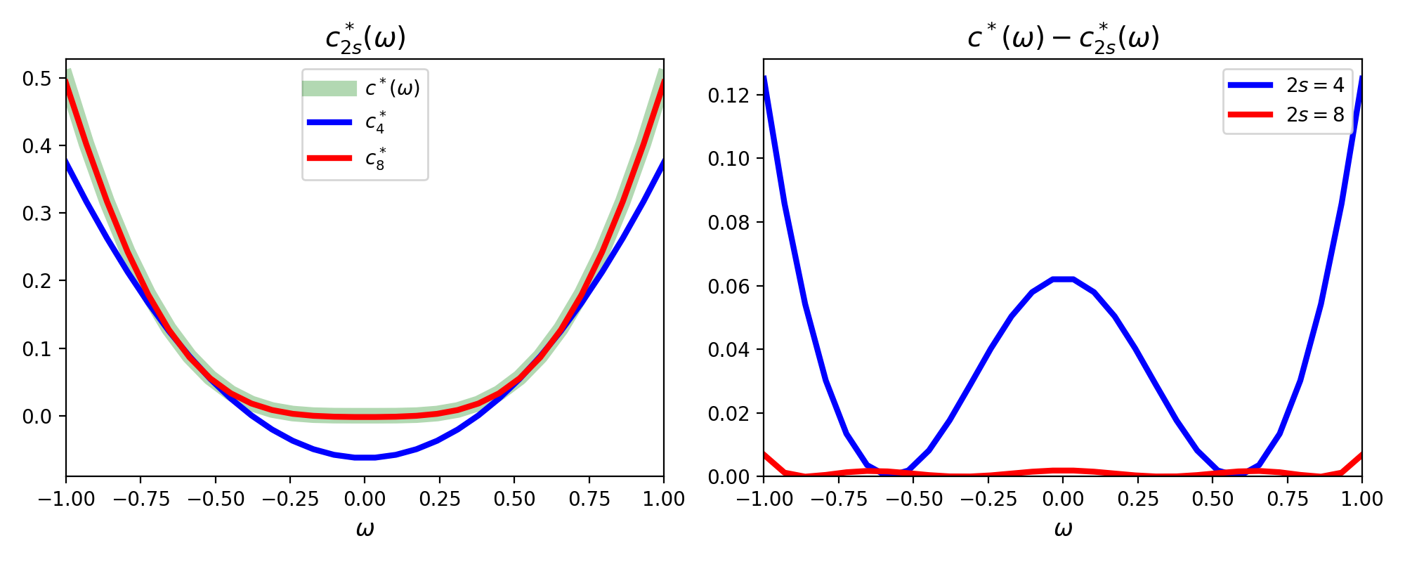
We now proceed with formulating and solving the degree- primal S-SOS SDP (Equation 2). We assume that is parameterized by a polynomial of degree in . Observe that this class of functions is not large enough to contain the true function .
We choose and use the standard monomial basis in , we have the feature maps and , since there are unique monomials of up to degree- in variables. These assumptions together enable us to explicitly write a SOS SDP in terms of coefficient matching. Note that we must assume some noise distribution . For this section, we present results assuming . We solve the resulting SDP in CVXPY using Legendre quadrature with zeroes on to evaluate the objective . In fact, sample points suffice to exactly integrate polynomials of degree .
We solve the SDP for two different levels of the hierarchy, and (producing lower-bound polynomials of degree and respectively), and plot the lower bound functions vs the true lower bound as well as the optimality gap to the true lower bound in Fig.2.
A.6.3 Convergence of lower bound as degree increases
To solve the S-SOS SDP in practice, we must choose a maximum degree for the SOS function and the lower-bounding function , which are both restricted to be polynomials. Indeed, a larger not only increases the dimension of our basis function but also the complexity of the resulting SDP. We would expect that as , i.e. the optimal value of the degree- S-SOS SDP (Equation 4) converges to that of the “minimizing distribution” optimization problem (Equation 3).
In particular, note that in the standard SOS hierarchy we typically find finite convergence (exact agreement at some degree ). However, in S-SOS, we thus far have only a guarantee of asymptotic convergence, as each finite-degree S-SOS SDP solves for a polynomial approximation to the optimal lower bound . In Figure 1, we illustrate the primal S-SOS SDP objective values
for a given level of the hierarchy (a chosen degree for the basis ) and their convergence towards the optimal objective value
for the simple quadratic potential, assuming with . We note that in the log-linear plot (right) we have a “hinge”-type curve, with a linear decay (in logspace) and then flattening completely. This suggests perhaps that in realistic scenarios the degree needed to achieve a close approximation is very low, lower than suggested by our bounds. The flattening that occurs here is likely due to the numerical tolerance used in our solver (CVXPY/MOSEK), as increasing the tolerance also increases the asymptotic gap and decreases the degree at which the gap flattens out.
A.6.4 Effect of different noise distributions
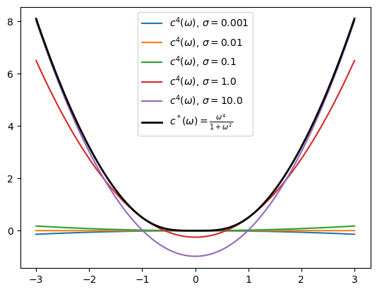
In the previous two sections, we assumed that . This enabled us to solve the primal exactly using Legendre quadrature of polynomials. Note that in Figure 1 we see that the lower-bounding for is a smooth polynomial that has curvature (i.e. sign matching that of the true minimum). This is actually not guaranteed, as we will see shortly.
In Figure 3, we present the lower-bounding functions achieved by degree-4 S-SOS by solving the dual for for varying widths . We can see that for small , the primal solution only cares about the lower-bound accuracy within a small region of , and the lower-bounding curve fails to “generalize” effectively outside the region of consideration.
A.7 S-SOS for sensor network localization
A.7.1 SDP formulation
Recall the form of :
Note that the function is exactly a degree-4 SOS polynomial, so it suffices to choose the degree-2 monomial basis containing elements as . That is, we have sensor positions in spatial dimensions and parameters for a total of variables.
Let the moment matrix be with elements defined as
for , which fully specifies the minimizing distribution as in Equation 4.
Our SDP is then of the form
where corresponds to the moment-matching constraints of Equation 4 and correspond to any possible hard equality constraints required to set the exact position (and uncertainty) of a sensor for all . represents the moment-matching constraints necessary for all moments w.r.t. and represents the constraints needed to set the exact positions of known sensor positions in (i.e. 1 constraint per sensor and dimension, 2 each for mean and variance).
A.7.2 Noise types
In this paper we focus on the linear uniform noise case, as it is a more accurate reflection of measurement noise in true SNL problems. Special robust estimation approaches may be needed to properly handle the outlier noise case.
-
•
Linear uniform noise: for a subset of edges we write , , and some noise scale we set. The same random variate may perturb any number of edges. Otherwise the observed distances are the true distances.
-
•
Outlier uniform noise: for a subset of edges we ignore any information in the actual measurement , where is the physical dimension of the problem, i.e. .
A.7.3 Algorithms: S-SOS and MCPO
Here we explicitly formulate MCPO and S-SOS as algorithms. Let and use the standard monomial basis. We write . Our objective is to approximate for all , with a view towards maximizing for sampled from some probability density .
MCPO (Algorithm 1) simply samples and finds a set of tuples where the optimal minimizer is computed using a local optimization scheme (we use BFGS).
S-SOS (Algorithm 2) via solving the dual (Equation 4) is also detailed below.
A.7.4 Cluster basis hierarchy
Recall from Section 2.2.2 that we defined the cluster basis hierarchy using body order and maximum degree per variable . In this section, we review the additional modifications needed to scale S-SOS for SNL.
In SNL, is by design a degree polynomial in , with interactions of body order (due to the interactions) and maximum individual variable degree . Written this way, we want to only consider monomial terms with , , and .
To sparsify our problem, we start with some -clustering ( clusters, mutually-exclusive) of the sensor set . This clustering can be considered as leveraging some kind of “coarse“ information about which sensors are close to each other. For example, just looking at the polynomial enables us to see which sensors must be interacting.
Assume that there is some a priori clustering given to us. We denote as the subset of the variables restricted to the cluster , i.e. . Moreover, let be a graph where the vertices correspond to the clusters and the edges correspond to known cluster-cluster interactions.
The SOS part of the function may then be approximated as the sum of dense intra-cluster interactions and sparse inter-cluster interactions, where the cluster-cluster interactions are given exactly by edges in the graph :
where are symmetric PSD matrices and are rectangular matrices where we require . for here behaves as before and denotes the basis function generated by all combinations of monomials with degree . Notice that this is a strict reduction from the standard Lasserre hierarchy at the same degree , since in general the standard basis on the full variable set will contain terms that mix variables from two different clusters that may not have an edge connecting them.
Efficiency gains in the SDP solve occur when we constrain certain of the off-diagonal blocks to be zero, i.e. the graph is sparse in cluster-cluster interactions. As we can see from the block decomposition written above, this resembles block sparsity on the matrix . We may interpret the above scheme as having a hierarchical structure out to depth 2, where we have dense interactions at the lowest level and sparse interactions aggregating them. In full generality, the resulting hierarchical sparsity in may be interpreted as generating a chordal , which is known to admit certain speed-ups in SDP solvers [41].
When attempting to solve an SNL problem in the cluster basis instead of the full basis, we need to throw away terms in the potential that correspond to cross-terms that are “ignored” by the particular cluster basis we chose. The resulting polynomial has fewer terms and produces a cluster basis SDP that is easier to solve, but generally less accurate due to the sparser connectivity.
In particular, for the rows in Table 1 that have , we do a -means clustering of the ground-truth sensor positions and use those sensor labels to create our partitioning of the sensors. We connect every cluster using plus-one (including the wrap-around one) connections, so that the cluster-cluster connectivity graph has edges. We then use this information to throw out observed distances from the set and from the full basis function . See our code for complete details.
A.7.5 Hard equality constraints
The sensor-anchor terms in Equation 7 are added to make the problem easier, because by adding them now each sensor no longer needs to rely only on a local neighborhood of sensors to localize itself, but can also use its position relative to some known anchor. When we remove them entirely, we need to incorporate hard equality constraints between certain sensors and known “anchor” positions. This fixes certain known sensors but lets every other sensor be unrooted, defined only relative to other sensors (and potentially an anchor if it is within the sensing radius).
To deal with the equality constraints where we set the exact position of a sensor , we solve the dual Equation 4 and implement them as equality constraints on the moment matrix, i.e. for the basis element we may set . Note that we also need to set so for we add the equality constraint .
A.7.6 Solution extraction
Once the dual SDP has been solved, we extract the moment matrix and can easily recover the point and uncertainty estimates for the sensor positions by inspecting the appropriate entries corresponding to and corresponding to .
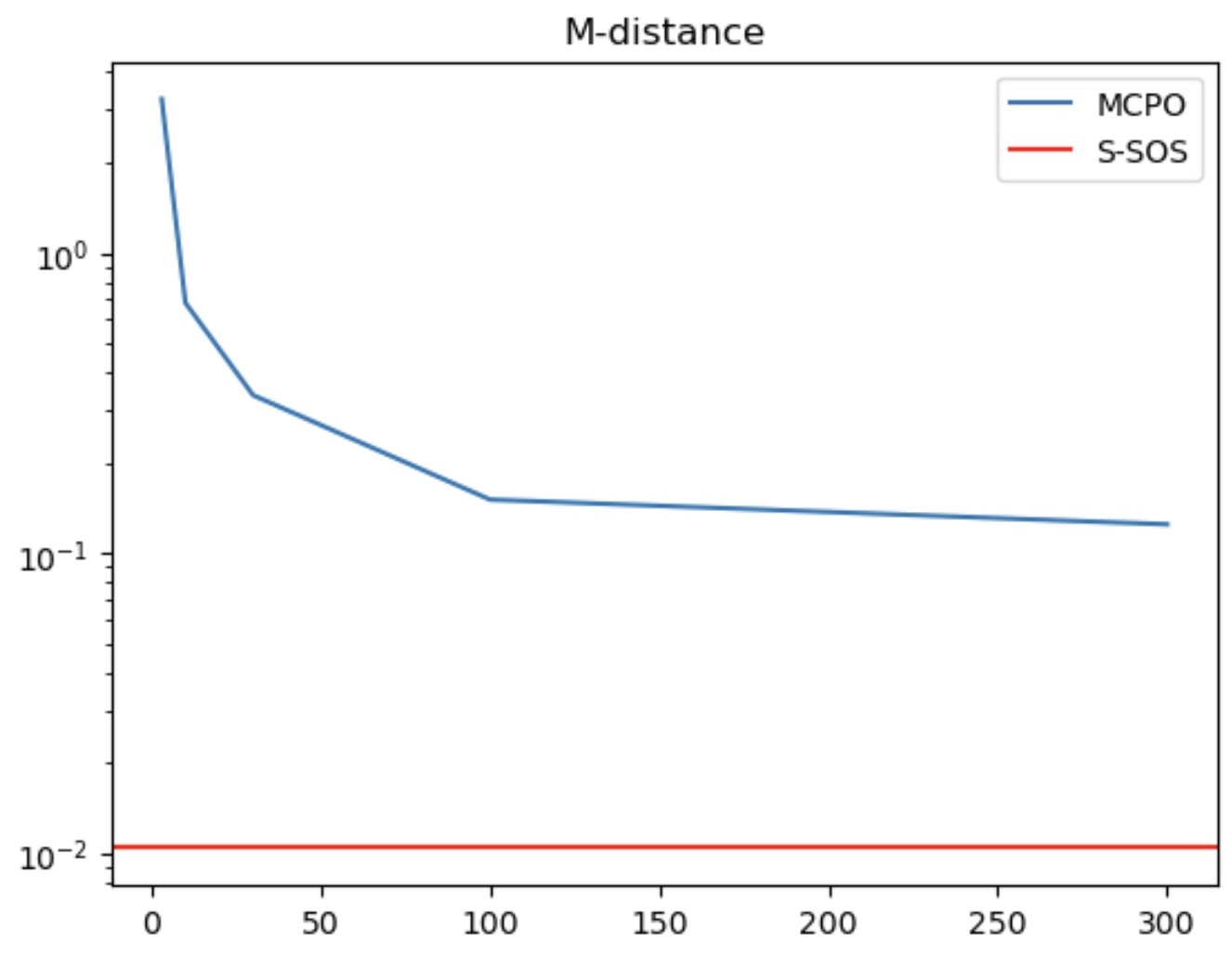
A.7.7 Impact of using MCPO with varying numbers of samples
In Figure 4 we can see how varies as we scale the number of samples used in the MCPO estimate of the empirical mean/covariance of the recovered solutions. In this particular example, the runtime of the S-SOS estimate was 0.3 seconds, comparing to 30 seconds for the MCPO point. Despite taking 100x longer, the MCPO solution recovery still dramatically underperforms S-SOS in . This reflects the poor performance of local optimization methods vs. a global optimization method (when it is available).
A.7.8 Scalability
The largest 2D SNL experiment we could run had sensors, clusters, and noise parameters. This generated variables and basis elements in the naive construction, which was reduced to after our application of the cluster basis, giving us . A single solve in CVXPY (MOSEK) took 30 minutes on our workstation (2x Intel Xeon 6130 Gold and 256GB of RAM). We attempted a run with sensors and clusters and noise parameters, but the process failed due to OOM constraints. Thus, we report the largest experiment that succeeded.