Mirror and Preconditioned Gradient Descent in Wasserstein Space

Abstract

As the problem of minimizing functionals on the Wasserstein space encompasses many applications in machine learning, different optimization algorithms on $\mathbb{R}^{d}$ have received their counterpart analog on the Wasserstein space. We focus here on lifting two explicit algorithms: mirror descent and preconditioned gradient descent. These algorithms have been introduced to better capture the geometry of the function to minimize and are provably convergent under appropriate (namely relative) smoothness and convexity conditions. Adapting these notions to the Wasserstein space, we prove guarantees of convergence of some Wasserstein-gradient-based discrete-time schemes for new pairings of objective functionals and regularizers. The difficulty here is to carefully select along which curves the functionals should be smooth and convex. We illustrate the advantages of adapting the geometry induced by the regularizer on ill-conditioned optimization tasks, and showcase the improvement of choosing different discrepancies and geometries in a computational biology task of aligning single-cells.

1 Introduction

Minimizing functionals on the space of probability distributions has become ubiquitous in Machine Learning for e.g. sampling [12, 118], generative modeling [13] or learning neural networks [33, 83], and is a challenging task as it is an infinite-dimensional problem. Wasserstein gradient flows [4] provide an elegant way to solve such problems on the Wasserstein space, i.e., the space of probability distributions with bounded second moment, equipped with the 2-Wasserstein distance from optimal transport (OT). These flows provide continuous paths of distributions decreasing the objective functional and can be seen as analog to Euclidean gradient flows [103]. Their implicit time discretization, referred to as the JKO scheme [61], has been studied in depth [88, 1, 25, 103]. In contrast, explicit schemes, despite being easier to implement, have been less investigated. Most previous works focus on the optimization of a specific objective functional with a time-discretation of its gradient flow with the 2-Wasserstein metrics. For instance, the forward Euler discretization leads to the Wasserstein gradient descent. The latter takes the form of gradient descent (GD) on the position of particles for functionals with a closed-form over discrete measures, e.g. Maximum Mean Discrepancy (MMD), which can be of interest to train neural networks [6]. For objectives involving absolutely continuous measures, such as the Kullback-Leibler (KL) divergence for sampling, other discretizations can be easily computed such as the Unadjusted Langevin Algorithm (ULA) [99]. This leaves the question open of assessing the theoretical and empirical performance of other optimization algorithms relying on alternative geometries and time-discretizations.

In the optimization community, a recent line of works has focused on extending the methods and convergence theory beyond the Euclidean setting by using more general costs for the gradient descent scheme [70]. For instance, mirror descent (MD), originally introduced by Nemirovskij and Yudin [85] to solve constrained convex problems, uses a cost that is a divergence defined by a Bregman potential [11]. Mirror descent benefits from convergence guarantees for objective functions that are relatively smooth in the geometry induced by the (Bregman) divergence [81], even if they do not have a Lipschitz gradient, i.e., are not smooth in the Euclidean sense. More recently, a closely related scheme, namely preconditioned gradient descent, was introduced in [82]. It can be seen as a dual version of the mirror descent algorithm, where the role of the objective function and Bregman potential are exchanged. In particular, its convergence guarantees can be obtained under relative smoothness and convexity of the Fenchel transform of the potential, with respect to the objective. This algorithm appears more efficient to minimize the gradient magnitude than mirror descent [63]. The flexible choice of the Bregman divergence used by these two schemes enables to design or discover geometries that are potentially more efficient.

Mirror descent has already attracted attention in the sampling community, and some popular algorithms have been extended in this direction. For instance, ULA was adapted into the Mirror Langevin algorithm [58, 120, 30, 59, 3, 72]. Other sampling algorithms have received their counterpart mirror versions such as the Metropolis Adjusted Langevin Algorithm [108], diffusion models [75], Stein Variational Gradient Descent (SVGD) [106], or even Wasserstein gradient descent [105]. Preconditioned Wasserstein gradient descent has been also recently proposed for specific geometries in [41, 29] to minimize the KL in a more efficient way, but without an analysis in discrete time. All the previous references focus on optimizing the KL as an objective, while Wasserstein gradient flows have been studied in machine learning for different functionals such as more general $f$-divergences [5, 86], interaction energies [71], MMDs [6, 67, 56, 55] or Sliced-Wasserstein (SW) distances [18, 79, 42, 15]. In this work, we propose to bridge this gap by providing a general convergence theory of both mirror and preconditioned gradient descent schemes for general target functionals, and investigate as well empirical benefits of alternative transport geometries for optimizing functionals on the Wasserstein space. We emphasize that the latter is different from [8, 62], wherein mirror descent is defined in the Radon space of probability distributions, using the flat geometry defined by TV or $L^{2}$ norms on measures, see Appendix A for more details.

Contributions.

We are interested in minimizing a functional $\mathcal{F}:\mathcal{P}_{2}(\mathbb{R}^{d})\to\mathbb{R}\cup\{+\infty\}$ over probability distributions, through schemes of the form, for $k\geq 0$,

$$\mathrm{T}_{k+1}=\operatorname*{argmin}_{\mathrm{T}\in L^{2}(\mu_{k})}\ \langle\nabla_{\mathrm{W}_{2}}\mathcal{F}(\mu_{k}),\mathrm{T}-\mathrm{Id}\rangle_{L^{2}(\mu_{k})}+\frac{1}{\tau}\mathrm{d}(\mathrm{T},\mathrm{Id}),\quad\mu_{k+1}=(\mathrm{T}_{k+1})_{\#}\mu_{k},$$ (1)

with different costs $\mathrm{d}:L^{2}(\mu_{k})\times L^{2}(\mu_{k})\to\mathbb{R}_{+}$, and in providing convergence conditions. While we can recover a map $\bar{\mathrm{T}}=\mathrm{T}_{k}\circ\mathrm{T}_{k-1}\dots\circ\mathrm{T}_{1}$ such that $\mu_{k}=\bar{\mathrm{T}}_{\#}\mu_{0}$, the scheme (1) proceeds by successive regularized linearizations retaining the Wasserstein structure, since the tangent space to $\mathcal{P}_{2}(\mathbb{R}^{d})$ at $\mu$ is a subset of $L^{2}(\mu)$ [89]. This paper is organized as follows. In Section 2, we provide some background on Bregman divergences and differentiability over the Wasserstein space. In Section 3, we consider Bregman divergences on $L^{2}(\mu)$ for the cost in (1), generalizing the mirror descent scheme to the Wasserstein space. In Section 4, we consider alternative costs in (1), that are analogous to OT distances with translation-invariant cost, extending the dual space preconditioning scheme to the latter space. Finally, in Section 5, we apply the two schemes to different objective functionals, including standard free energy functionals such as interaction energies and KL divergence, but also to Sinkhorn divergences [47] or SW [95, 16] with polynomial preconditioners on single-cell datasets.

Notation. Consider the set $\mathcal{P}_{2}(\mathbb{R}^{d})$ of probability measures $\mu$ on $\mathbb{R}^{d}$ with finite second moment and $\mathcal{P}_{2,\mathrm{ac}}(\mathbb{R}^{d})\subset\mathcal{P}_{2}(\mathbb{R}^{d})$ its subset of absolutely continuous probability measures with respect to the Lebesgue measure. For any $\mu\in\mathcal{P}_{2}(\mathbb{R}^{d})$, we denote by $L^{2}(\mu)$ the Hilbert space of functions $f:\mathbb{R}^{d}\to\mathbb{R}^{d}$ such that $\int\|f\|^{2}\mathrm{d}\mu<\infty$ equipped with the norm $\|\cdot\|_{L^{2}(\mu)}$ and inner product $\langle\cdot,\cdot\rangle_{L^{2}(\mu)}$. For a Hilbert space $X$, the Fenchel transform of $f:X\to\mathbb{R}$ is $f^{*}(y)=\sup_{x\in X}\ \langle x,y\rangle-f(x)$. Given a measurable map $\mathrm{T}:\mathbb{R}^{d}\to\mathbb{R}^{d}$ and $\mu\in\mathcal{P}_{2}(\mathbb{R}^{d})$, $\mathrm{T}_{\#}\mu$ is the pushforward measure of $\mu$ by $\mathrm{T}$; and $\mathrm{T}\star\mu=\int\mathrm{T}(\cdot-x)\mathrm{d}\mu(x)$. For $\mu,\nu\in\mathcal{P}_{2}(\mathbb{R}^{d})$, the 2-Wasserstein distance is $\mathrm{W}_{2}^{2}(\mu,\nu)=\inf_{\gamma\in\Pi(\mu,\nu)}\int\|x-y\|^{2}\ \mathrm{d}\gamma(x,y)$, where $\Pi(\mu,\nu)$ is the set of couplings between $\mu$ and $\nu$, and we denote by $\Pi_{o}(\mu,\nu)$ the set of optimal couplings. We refer to the metric space $(\mathcal{P}_{2}(\mathbb{R}^{d}),\mathrm{W}_{2})$ as the Wasserstein space.

2 Background

In this section, we fix $\mu\in\mathcal{P}_{2}(\mathbb{R}^{d})$ and introduce first the Bregman divergence on $L^{2}(\mu)$ along with the notions of relative convexity and smoothness that will be crucial in the analysis of the optimization schemes. Then, we introduce the differential structure and computation rules for differentiating a functional $\mathcal{F}:\mathcal{P}_{2}(\mathbb{R}^{d})\to\mathbb{R}$ along curves and discuss notions of convexity on $\mathcal{P}_{2}(\mathbb{R}^{d})$. We refer the reader to Appendix B and Appendix C for more details on $L^{2}(\mu)$ and the Wasserstein space respectively. Finally, we introduce the mirror descent and preconditioned gradient descent on $\mathbb{R}^{d}$.

Bregman divergence on $L^{2}(\mu)$.

Frigyik et al. [50, Definition 2.1] defined the Bregman divergence of Fréchet differentiable functionals. In our case, we only need Gâteaux differentiability. In this paper, $\nabla$ refers to the Gâteaux differential, which coincides with the Fréchet derivative if the latter exists.

Definition 1.

Let $\phi_{\mu}:L^{2}(\mu)\to\mathbb{R}$ be convex and continuously Gâteaux differentiable. The Bregman divergence is defined for all $\mathrm{T},\mathrm{S}\in L^{2}(\mu)$ as $\mathrm{d}_{\phi_{\mu}}(\mathrm{T},\mathrm{S})=\phi_{\mu}(\mathrm{T})-\phi_{\mu}(\mathrm{S})-\langle\nabla\phi_{\mu}(\mathrm{S}),\mathrm{T}-\mathrm{S}\rangle_{L^{2}(\mu)}.$

We use the same definition on $\mathbb{R}^{d}$. The map $\phi_{\mu}$ (respectively $\nabla\phi_{\mu}$) in the definition of $\mathrm{d}_{\phi_{\mu}}$ above is referred to as the Bregman potential (respectively mirror map). If $\phi_{\mu}$ is strictly convex, then $\mathrm{d}_{\phi_{\mu}}$ is a valid Bregman divergence, i.e. it is positive and separates maps $\mu$-almost everywhere (a.e.). In particular, for $\phi_{\mu}(\mathrm{T})=\frac{1}{2}\|\mathrm{T}\|_{L^{2}(\mu)}^{2}$, we recover the $L^{2}$ norm as a divergence $\mathrm{d}_{\phi_{\mu}}(\mathrm{T},\mathrm{S})=\frac{1}{2}\|\mathrm{T}-\mathrm{S}\|_{L^{2}(\mu)}^{2}$. Bregman divergences have received a lot of attention as they allow to define provably convergent schemes for functions which are not smooth in the standard (e.g. Euclidean) sense [81, 10], and thus for which gradient descent is not appropriate. These guarantees rely on the notion of relative smoothness and relative convexity [81, 82], which we introduce now on $L^{2}(\mu)$.

Definition 2 (Relative smoothness and convexity).

Let $\psi_{\mu},\phi_{\mu}:L^{2}(\mu)\to\mathbb{R}$ convex and continuously Gâteaux differentiable. We say that $\psi_{\mu}$ is $\beta$-smooth (respectively $\alpha$-convex) relative to $\phi$ if and only if for all $\mathrm{T},\mathrm{S}\in L^{2}(\mu),\ \mathrm{d}_{\psi_{\mu}}(\mathrm{T},\mathrm{S})\leq\beta\mathrm{d}_{\phi_{\mu}}(\mathrm{T},\mathrm{S})$ (respectively $\mathrm{d}_{\psi_{\mu}}(\mathrm{T},\mathrm{S})\geq\alpha\mathrm{d}_{\phi_{\mu}}(\mathrm{T},\mathrm{S})$).

Similarly to the Euclidean case [81], relative smoothness and convexity are equivalent with respectively $\beta\phi_{\mu}-\psi_{\mu}$ and $\psi_{\mu}-\alpha\phi_{\mu}$ being convex (see Section B.2). Yet, proving the convergence of (1) requires only that these properties hold at specific functions (directions), a fact we will soon exploit.

In some situations, we need the $L^{2}$ Fenchel transform $\phi_{\mu}^{*}$ of $\phi_{\mu}$ to be differentiable, e.g. to compute its Bregman divergence $\mathrm{d}_{\phi_{\mu}^{*}}$. We show in Lemma 16 that a sufficient condition to satisfy this property is for $\phi_{\mu}$ to be strictly convex, lower semicontinuous and superlinear, i.e. $\lim_{\|\mathrm{T}\|\to\infty}\phi_{\mu}(\mathrm{T})/\|\mathrm{T}\|_{L^{2}(\mu)}=+\infty$. Moreover, in this case, $(\nabla\phi_{\mu})^{-1}=\nabla\phi_{\mu}^{*}$. When needed, we will suppose that $\phi_{\mu}$ satisfies this.

Differentiability on $(\mathcal{P}_{2}(\mathbb{R}^{d}),\mathrm{W}_{2})$.

Let $\mathcal{F}:\mathcal{P}_{2}(\mathbb{R}^{d})\to\mathbb{R}\cup\{+\infty\}$, and denote $D(\mathcal{F})=\{\mu\in\mathcal{P}_{2}(\mathbb{R}^{d}),\ \mathcal{F}(\mu)<+\infty\}$ the domain of $\mathcal{F}$ and $D(\tilde{\mathcal{F}}_{\mu})=\{\mathrm{T}\in L^{2}(\mu),\ \mathrm{T}_{\#}\mu\in D(\mathcal{F})\}$ the domain of $\tilde{\mathcal{F}}_{\mu}$ defined as $\tilde{\mathcal{F}}_{\mu}(\mathrm{T}):=\mathcal{F}(\mathrm{T}_{\#}\mu)$ for all $\mathrm{T}\in L^{2}(\mu)$. In the following, we use the differential structure of $(\mathcal{P}_{2}(\mathbb{R}^{d}),\mathrm{W}_{2})$ introduced in [17, Definition 2.8], and we say that $\nabla_{\mathrm{W}_{2}}\mathcal{F}(\mu)$ is a Wasserstein gradient of $\mathcal{F}$ at $\mu\in D(\mathcal{F})$ if for any $\nu\in\mathcal{P}_{2}(\mathbb{R}^{d})$ and any optimal coupling $\gamma\in\Pi_{o}(\mu,\nu)$,

$$\mathcal{F}(\nu)=\mathcal{F}(\mu)+\int\langle\nabla_{\mathrm{W}_{2}}\mathcal{F}(\mu)(x),y-x\rangle\ \mathrm{d}\gamma(x,y)+o\big{(}\mathrm{W}_{2}(\mu,\nu)\big{)}.$$ (2)

If such a gradient exists, then we say that $\mathcal{F}$ is $\mathrm{W}_{2}$-differentiable at $\mu$ [17, 69]. The differentiability of $\tilde{\mathcal{F}}_{\mu}$ and $\mathcal{F}$ are clearly related. Indeed, if $\mathcal{F}$ satisfies (2), $\tilde{\mathcal{F}}_{\mu}$ defined as above is Fréchet differentiable (Proposition 8). Moreover there is a unique gradient belonging to the tangent space of $\mathcal{P}_{2}(\mathbb{R}^{d})$ verifying $\eqref{eq:wass_diff}$ [69, Proposition 2.5]. We will always restrict ourselves to this particular gradient, as it satisfies, for all $\mathrm{S}\in D(\tilde{\mathcal{F}}_{\mu})$, $\nabla\tilde{\mathcal{F}}_{\mu}(\mathrm{S})=\nabla_{\mathrm{W}_{2}}\mathcal{F}(\mathrm{S}_{\#}\mu)\circ\mathrm{S}$, see Section C.1. $\mathrm{W}_{2}$-differentiable functionals include $c$-Wasserstein costs, potential energies $\mathcal{V}(\mu)=\int V\mathrm{d}\mu$ or interaction energies $\mathcal{W}(\mu)=\iint W(x-y)\ \mathrm{d}\mu(x)\mathrm{d}\mu(y)$ for $V$ and $W$ differentiable and $L$-smooth [69, Section 2.4]. However, entropy functionals, e.g. the negative entropy defined as $\mathcal{H}(\mu)=\int\log\big(\rho(x)\big{missing})\mathrm{d}\mu(x)$ for distributions $\mu$ admitting a density $\rho$ w.r.t. the Lebesgue measure, are not $\mathrm{W}_{2}$-differentiable. In this case, we can consider subgradients $\nabla_{\mathrm{W}_{2}}\mathcal{F}(\mu)$ at $\mu$ for which (2) becomes an inequality. To guarantee that the Wasserstein subgradient is not empty, we need $\rho$ to satisfy some Sobolev regularity, see e.g. [4, Theorem 10.4.13] or [100]. Then, if $\nabla\log\rho\in L^{2}(\mu)$, the only subgradient of $\mathcal{H}$ in the tangent space is $\nabla_{\mathrm{W}_{2}}\mathcal{H}(\mu)=\nabla\log\rho$, see [4, Theorem 10.4.17] and [44, Proposition 4.3]. Free energies write as sums of potential, interaction and entropy terms [102, Chapter 7]. It is notably the case for the KL to a fixed target distribution, that is the sum of a potential and entropy term [118], or the MMD as a sum of a potential and interaction term [6].

Examples of functionals.

The definitions of Bregman divergences on $L^{2}(\mu)$ and of $\mathrm{W}_{2}$-differentiability enable us to consider alternative Bregman potentials than the $L^{2}(\mu)$-norm mentioned above. For instance, for $V$ and $W$ convex, differentiable and $L$-smooth with $W$ even, we can use potential energies $\phi_{\mu}^{V}(\mathrm{T}):=\mathcal{V}(\mathrm{T}_{\#}\mu)$, for which $\mathrm{d}_{\phi_{\mu}^{V}}(\mathrm{T},\mathrm{S})=\int\mathrm{d}_{V}\big{(}\mathrm{T}(x),\mathrm{S}(x)\big{)}\mathrm{d}\mu(x)$ where $\mathrm{d}_{V}$ is the Bregman divergence of $V$ on $\mathbb{R}^{d}$. Notice that $\phi_{\mu}(\mathrm{T})=\frac{1}{2}\|\mathrm{T}\|^{2}_{L^{2}(\mu)}$ is a specific example of a potential energy where $V=\frac{1}{2}\|\cdot\|^{2}$. In particular, we have $\nabla_{\mathrm{W}_{2}}\mathcal{V}(\mu)=\nabla V$. We will also consider interaction energies $\phi_{\mu}^{W}(\mathrm{T}):=\mathcal{W}(\mathrm{T}_{\#}\mu)$, for which $\mathrm{d}_{\phi_{\mu}^{W}}(\mathrm{T},\mathrm{S})=\iint\mathrm{d}_{W}\big{(}\mathrm{T}(x)-\mathrm{T}(x^{\prime}),\mathrm{S}(x)-\mathrm{S}(x^{\prime})\big{)}\mathrm{d}\mu(x)\mathrm{d}\mu(x^{\prime})$ (see Section I.3). In that case, $\nabla_{\mathrm{W}_{2}}\mathcal{W}(\mu)=\nabla W\star\mu$. We will also use $\phi_{\mu}^{\mathcal{H}}(\mathrm{T})=\mathcal{H}(\mathrm{T}_{\#}\mu)$ with $\mathcal{H}$ the negative entropy. Note that Bregman divergences on the Wasserstein space using these functionals were proposed by Li [73], but only for $\mathrm{S}=\mathrm{Id}$ and OT maps $\mathrm{T}$.

Convexity and smoothness in $(\mathcal{P}_{2}(\mathbb{R}^{d}),\mathrm{W}_{2})$.

In order to study the convergence of gradient flows and their discrete-time counterparts, it is important to have suitable notions of convexity and smoothness. On $(\mathcal{P}_{2}(\mathbb{R}^{d}),\mathrm{W}_{2})$, different such notions have been proposed based on specific choices of curves. The most popular one is to require the functional $\mathcal{F}$ to be $\alpha$-convex along geodesics (see Definition 11), which are of the form $\mu_{t}=\big{(}(1-t)\mathrm{Id}+t\mathrm{T}_{\mu_{0}}^{\mu_{1}}\big{)}_{\#}\mu_{0}$ if $\mu_{0}\in\mathcal{P}_{2,\mathrm{ac}}(\mathbb{R}^{d})$ and $\mu_{1}\in\mathcal{P}_{2}(\mathbb{R}^{d})$, with $\mathrm{T}_{\mu_{0}}^{\mu_{1}}$ the OT map between them. In that setting,

$$\frac{\alpha}{2}\mathrm{W}_{2}^{2}(\mu_{0},\mu_{1})=\frac{\alpha}{2}\|\mathrm{T}_{\mu_{0}}^{\mu_{1}}-\mathrm{Id}\|_{L^{2}(\mu_{0})}^{2}\leq\mathcal{F}(\mu_{1})-\mathcal{F}(\mu_{0})-\langle\nabla_{\mathrm{W}_{2}}\mathcal{F}(\mu_{0}),\mathrm{T}_{\mu_{0}}^{\mu_{1}}-\mathrm{Id}\rangle_{L^{2}(\mu_{0})}.$$ (3)

For instance, free energies such as potential or interaction energies with convex $V$ or $W$, or the negative entropy, are convex along geodesics [102, Section 7.3]. However, some popular functionals, such as the 2-Wasserstein distance $\mu\mapsto\frac{1}{2}\mathrm{W}_{2}^{2}(\mu,\eta)$ itself, for a given $\eta\in\mathcal{P}_{2}(\mathbb{R}^{d})$, are not convex along geodesics. Instead Ambrosio et al. [4, Theorem 4.0.4] showed that it was sufficient for the convergence of the gradient flow to be convex along other curves, e.g. along particular generalized geodesics for the 2-Wasserstein distance [4, Lemma 9.2.7], which, for $\mu,\nu\in\mathcal{P}_{2}(\mathbb{R}^{d})$, are of the form $\mu_{t}=\big{(}(1-t)\mathrm{T}_{\eta}^{\mu}+t\mathrm{T}_{\eta}^{\nu}\big{)}_{\#}\eta$ for $\mathrm{T}_{\eta}^{\mu}$, $T_{\eta}^{\nu}$ OT maps from $\eta$ to $\mu$ and $\nu$. Observing that for $\phi_{\mu}(\mathrm{T})=\frac{1}{2}\|\mathrm{T}\|_{L^{2}(\mu)}^{2}$, we can rewrite (3) as $\alpha\mathrm{d}_{\phi_{\mu_{0}}}(\mathrm{T}_{\mu_{0}}^{\mu_{1}},\mathrm{Id})\leq\mathrm{d}_{\tilde{\mathcal{F}}_{\mu_{0}}}(\mathrm{T}_{\mu_{0}}^{\mu_{1}},\mathrm{Id})$, we see that being convex along geodesics boils down to being convex in the $L^{2}$ sense for $\mathrm{S}=\mathrm{Id}$ and $\mathrm{T}$ chosen as an OT map. This observation motivates us to consider a more refined notion of convexity along curves.

Definition 3.

Let $\mu\in\mathcal{P}_{2}(\mathbb{R}^{d})$, $\mathrm{T},\mathrm{S}\in L^{2}(\mu)$ and for all $t\in[0,1]$, $\mu_{t}=(\mathrm{T}_{t})_{\#}\mu$ with $\mathrm{T}_{t}=(1-t)\mathrm{S}+t\mathrm{T}$. We say that $\mathcal{F}:\mathcal{P}_{2}(\mathbb{R}^{d})\to\mathbb{R}$ is $\alpha$-convex (resp. $\beta$-smooth) relative to $\mathcal{G}:\mathcal{P}_{2}(\mathbb{R}^{d})\to\mathbb{R}$ along $t\mapsto\mu_{t}$ if for all $s,t\in[0,1]$, $\mathrm{d}_{\tilde{\mathcal{F}}_{\mu}}(\mathrm{T}_{s},\mathrm{T}_{t})\geq\alpha\mathrm{d}_{\tilde{\mathcal{G}}_{\mu}}(\mathrm{T}_{s},\mathrm{T}_{t})$ (resp. $\mathrm{d}_{\tilde{\mathcal{F}}_{\mu}}(\mathrm{T}_{s},\mathrm{T}_{t})\leq\beta\mathrm{d}_{\tilde{\mathcal{G}}_{\mu}}(\mathrm{T}_{s},\mathrm{T}_{t})$).

Notice that in contrast with Definition 2, Definition 3 is stated for a fixed distribution $\mu$ and directions ($\mathrm{S},\mathrm{T}$), and involves comparisons between Bregman divergences depending on $\mu$ and curves $(\mathrm{T}_{s})_{s\in[0,1]}$ depending on $\mathrm{S},\mathrm{T}$. The larger family of $\mathrm{S}$ and $\mathrm{T}$ for which Definition 3 holds, the more restricted is the notion of convexity of $\mathcal{F}-\alpha\mathcal{G}$ (resp. of $\beta\mathcal{G}-\mathcal{F}$) on $\mathcal{P}_{2}(\mathbb{R}^{d})$. For instance, 2-Wasserstein generalized geodesics with anchor $\eta\in\mathcal{P}_{2}(\mathbb{R}^{d})$ correspond to considering $\mathrm{S},\mathrm{T}$ as all the OT maps originating from $\eta$, among which geodesics are particular cases when taking $\eta=\mu$ (hence $\mathrm{S}=\mathrm{Id}$). If we furthermore ask for $\alpha$-convexity to hold for all $\mu\in\mathcal{P}_{2}(\mathbb{R}^{d})$ and $\mathrm{T},\mathrm{S}\in L^{2}(\mu)$ (i.e., not only OT maps), then we recover the convexity along acceleration free-curves as introduced in [109, 91, 27]. Our motivation behind Definition 3 is that the convergence proofs of MD and preconditioned GD require relative smoothness and convexity properties to hold only along specific curves.

Mirror (MD) and preconditioned gradient descent (PGD) on $\mathbb{R}^{d}$.

These schemes read respectively as $\nabla\phi(x_{k+1})-\nabla\phi(x_{k})=-\tau\nabla f(x_{k})$ [11] and $y_{k+1}-y_{k}=-\tau\nabla h^{*}\big{(}\nabla g(y_{k})\big{)}$ [82], where the objectives $f,g$ and the regularizers $h,\phi$ are convex $C^{1}$ functions from $\mathbb{R}^{d}$ to $\mathbb{R}$. The algorithms are closely related since, using the Fenchel transform and setting $g=\phi^{*}$ and $h^{*}=f$, we see that, for $y=\nabla\phi(x)$, the two schemes are equivalent when permuting the roles of the objective and of the regularizer. For MD, convergence of $f$ is ensured if $f$ is both $\nicefrac{{1}}{{\tau}}$-smooth and $\alpha$-convex relative to $\phi$ [81, Theorem 3.1]. Concerning PGD, assuming that $h,g$ are Legendre, $g(y_{n})$ converges to the minimum of $g$ if $h^{*}$ is both $\nicefrac{{1}}{{\tau}}$-smooth and $\alpha$-convex relative to $g^{*}$ with $\alpha>0$ [82, Theorem 3.9].

3 Mirror descent

For every $\mu\in\mathcal{P}_{2}(\mathbb{R}^{d})$, let $\phi_{\mu}:L^{2}(\mu)\to\mathbb{R}$ be strictly convex, proper and differentiable and assume that the (sub)gradient $\nabla_{\mathrm{W}_{2}}\mathcal{F}(\mu)\in L^{2}(\mu)$ exists. In this section, we are interested in analyzing the scheme (1) where the cost $\mathrm{d}$ is chosen as a Bregman divergence, i.e. $\mathrm{d}_{\phi_{\mu}}$ as defined in Definition 1. This corresponds to a mirror descent scheme in $\mathcal{P}_{2}(\mathbb{R}^{d})$:

$$\mathrm{T}_{k+1}=\operatorname*{argmin}_{\mathrm{T}\in L^{2}(\mu_{k})}\ \mathrm{d}_{\phi_{\mu_{k}}}(\mathrm{T},\mathrm{Id})+\tau\langle\nabla_{\mathrm{W}_{2}}\mathcal{F}(\mu_{k}),\mathrm{T}-\mathrm{Id}\rangle_{L^{2}(\mu_{k})},\quad\mu_{k+1}=(\mathrm{T}_{k+1})_{\#}\mu_{k}.$$ (4)

Iterates of MD.

In all that follows, we assume that the iterates (4) exist, which is true e.g. for a superlinear $\phi_{\mu_{k}}$, since the objective is a sum of linear functions and of the continuous $\phi_{\mu_{k}}$. In the previous section, we have seen that the second term in the proximal scheme (4) can be interpreted as a linearization of the functional $\mathcal{F}$ at $\mu_{k}$ for Wasserstein (sub-)differentiable functionals. Now define for all $\mathrm{T}\in L^{2}(\mu_{k})$, $\mathrm{J}(\mathrm{T})=\mathrm{d}_{\phi_{\mu_{k}}}(\mathrm{T},\mathrm{Id})+\tau\langle\nabla_{\mathrm{W}_{2}}\mathcal{F}(\mu_{k}),\mathrm{T}-\mathrm{Id}\rangle_{L^{2}(\mu_{k})}$. Then, deriving the first order conditions of (4) as $\nabla\mathrm{J}(\mathrm{T}_{k+1})=0$, we obtain $\mu_{k}$-a.e.,

$$\nabla\phi_{\mu_{k}}(\mathrm{T}_{k+1})=\nabla\phi_{\mu_{k}}(\mathrm{Id})-\tau\nabla_{\mathrm{W}_{2}}\mathcal{F}(\mu_{k})\Longleftrightarrow\mathrm{T}_{k+1}=\nabla\phi_{\mu_{k}}^{*}\big{(}\nabla\phi_{\mu_{k}}(\mathrm{Id})-\tau\nabla_{\mathrm{W}_{2}}\mathcal{F}(\mu_{k})\big{)}.$$ (5)

Note that for $\phi_{\mu}(\mathrm{T})=\frac{1}{2}\|\mathrm{T}\|^{2}_{L^{2}(\mu)}$, the update (5) translates as $\mathrm{T}_{k+1}=\mathrm{Id}-\tau\nabla_{\mathrm{W}_{2}}\mathcal{F}(\mu_{k})$, and our scheme recovers Wasserstein gradient descent [32, 84]. This is analogous to mirror descent recovering gradient descent when the Bregman potential is chosen as the Euclidean squared norm in $\mathbb{R}^{d}$ [11]. We discuss in Section D.2 the continuous formulation of (4), showing it coincides with the gradient flow of the mirror Langevin [3, 119], the limit of the JKO scheme with Bregman groundcosts [97], Information Newton’s flows [115], or Sinkhorn’s flow [38] for specific choices of $\phi$ and $\mathcal{F}$.

Our proof of convergence of the mirror descent algorithm will require the Bregman divergence to satisfy the following property, which is reminiscent of conditions of optimality for couplings in OT.

Assumption 1.

For $\mu,\rho\in\mathcal{P}_{2,\mathrm{ac}}(\mathbb{R}^{d})$ and $\nu\in\mathcal{P}_{2}(\mathbb{R}^{d})$, setting $\mathrm{T}_{\phi_{\mu}}^{\mu,\nu}=\operatorname*{argmin}_{\mathrm{T}_{\#}\mu=\nu}\ \mathrm{d}_{\phi_{\mu}}(\mathrm{T},\mathrm{Id})$, $\mathrm{U}_{\phi_{\rho}}^{\rho,\nu}=\operatorname*{argmin}_{\mathrm{U}_{\#}\rho=\nu}\ \mathrm{d}_{\phi_{\rho}}(\mathrm{U},\mathrm{Id})$, the functional $\phi_{\mu}$ is such that, for any $\mathrm{S}\in L^{2}(\mu)$ satisfying $\mathrm{S}_{\#}\mu=\rho$, we have $\mathrm{d}_{\phi_{\mu}}(\mathrm{T}_{\phi_{\mu}}^{\mu,\nu},\mathrm{S})\geq\mathrm{d}_{\phi_{\rho}}(\mathrm{U}_{\phi_{\rho}}^{\rho,\nu},\mathrm{Id})$.

The inequality in 1 can be interpreted as follows: the "distance" between $\rho$ and $\nu$ is greater when observed from an anchor $\mu$ that differs from $\rho$ and $\nu$. We show that a sufficient condition for Bregman divergences to satisfy this assumption are the following conditions on the Bregman potential $\phi$.

Proposition 1.

Let $\mu,\rho\in\mathcal{P}_{2,\mathrm{ac}}(\mathbb{R}^{d})$ and $\nu\in\mathcal{P}_{2}(\mathbb{R}^{d})$. Let $\phi_{\mu}$ be a pushforward compatible functional, i.e. there exists $\phi:\mathcal{P}_{2}(\mathbb{R}^{d})\to\mathbb{R}$ such that for all $\mathrm{T}\in L^{2}(\mu)$, $\phi_{\mu}(\mathrm{T})=\phi(\mathrm{T}_{\#}\mu)$. Assume furthermore $\nabla_{\mathrm{W}_{2}}\phi(\mu)$ and $\nabla_{\mathrm{W}_{2}}\phi(\rho)$ invertible (on $\mathbb{R}^{d}$). Then, $\phi_{\mu}$ satisfies 1.

All the maps $\phi_{\mu}^{V}$, $\phi_{\mu}^{W}$ and $\phi_{\mu}^{\mathcal{H}}$ defined in Section 2 satisfy the assumptions of Proposition 1 under mild requirements, see Section D.1. The proof of Proposition 1 is given in Section H.1. It relies on the definition of an appropriate optimal transport problem

$$\mathrm{W}_{\phi}(\nu,\mu)=\inf_{\gamma\in\Pi(\nu,\mu)}\ \phi(\nu)-\phi(\mu)-\int\langle\nabla_{\mathrm{W}_{2}}\phi(\mu)(y),x-y\rangle\ \mathrm{d}\gamma(x,y),$$ (6)

and on the proof of existence of OT maps for absolutely continuous measures (see Proposition 13), which implies $\mathrm{W}_{\phi}(\nu,\mu)=\mathrm{d}_{\phi_{\mu}}(\mathrm{T}_{\phi_{\mu}}^{\mu,\nu},\mathrm{Id})$ with $\mathrm{T}_{\phi_{\mu}}^{\mu,\nu}$ defined as in 1. From there, we can conclude that $\phi_{\mu}$ satisfies 1. We notice that the corresponding transport problem recovers previously considered objects such as OT problems with Bregman divergence costs [24, 96], but is strictly more general (as our results pertain to the existence of OT maps), as detailed in Section D.1.

We now analyze the convergence of the MD scheme. Under a relative smoothness condition along curves generated by $\mathrm{S}=\mathrm{Id}$ and $\mathrm{T}=\mathrm{T}_{k+1}$ solutions of (4) for all $k\geq 0$, we derive the following descent lemma, which ensures that $\big{(}\mathcal{F}(\mu_{k})\big{)}_{k}$ is non-increasing. Its proof can be found in Section H.2 and relies on the three-point inequality [28], which we extended to $L^{2}(\mu)$ in Lemma 27.

Proposition 2.

Let $\beta>0$, $\tau\leq\frac{1}{\beta}$. Assume for all $k\geq 0$, $\mathcal{F}$ is $\beta$-smooth relative to $\phi$ along $t\mapsto\big{(}(1-t)\mathrm{Id}+t\mathrm{T}_{k+1}\big{)}_{\#}\mu_{k}$, which implies $\beta\mathrm{d}_{\phi_{\mu_{k}}}(\mathrm{T}_{k+1},\mathrm{Id})\geq\mathrm{d}_{\tilde{\mathcal{F}}_{\mu_{k}}}(\mathrm{T}_{k+1},\mathrm{Id})$. Then, for all $k\geq 0$,

$$\mathcal{F}(\mu_{k+1})\leq\mathcal{F}(\mu_{k})-\frac{1}{\tau}\mathrm{d}_{\phi_{\mu_{k}}}(\mathrm{Id},\mathrm{T}_{k+1}).$$ (7)

Assuming additionally the convexity of $\mathcal{F}$ along the curves $\mu_{t}=\big{(}(1-t)\mathrm{Id}+t\mathrm{T}_{\phi_{\mu}}^{\mu,\nu})_{\#}\mu$, $t\in[0,1]$ and that $\phi$ satisfies 1, we can obtain global convergence.

Proposition 3.

Let $\nu\in\mathcal{P}_{2}(\mathbb{R}^{d})$, $\alpha\geq 0$. Suppose 1 and the conditions of Proposition 2 hold, and that $\mathcal{F}$ is $\alpha$-convex relative to $\phi$ along the curves $t\mapsto\big{(}(1-t)\mathrm{Id}+t\mathrm{T}_{\phi_{\mu_{k}}}^{\mu_{k},\nu})_{\#}\mu_{k}$. Then, for all $k\geq 1$,

$$\mathcal{F}(\mu_{k})-\mathcal{F}(\nu)\leq\frac{\alpha}{\left(1-\tau\alpha\right)^{-k}-1}\mathrm{W}_{\phi}(\nu,\mu_{0})\leq\frac{1-\alpha\tau}{k\tau}\mathrm{W}_{\phi}(\nu,\mu_{0}).$$ (8)

Moreover, if $\alpha>0$, taking $\nu=\mu^{*}$ the minimizer of $\mathcal{F}$, we obtain a linear rate: for all $k\geq 0$, $\mathrm{W}_{\phi}(\mu^{*},\mu_{k})\leq\left(1-\tau\alpha\right)^{k}\mathrm{W}_{\phi}(\mu^{*},\mu_{0}).$

The proof of Proposition 3 can be found in Section H.3, and requires 1 to hold so that consecutive distances between iterates and the global minimizer telescope. This is not as direct as in the proofs of [81] over $\mathbb{R}^{d}$, because the minimization problem of each iteration (4) happens in a different space $L^{2}(\mu_{k})$. We discuss in Section 5 how to verify the relative smoothness and convexity on some examples. In particular, when both $\mathcal{F}$ and $\phi$ are potential energies, it is inherited from the relative smoothness and convexity on $\mathbb{R}^{d}$, and the conditions are similar with those for MD on $\mathbb{R}^{d}$. We also note that relative smoothness assumptions along descent directions as stated in Proposition 2 and relative strong convexity along optimal curves between the iterates and a minimizer as stated in Proposition 3 have been used already in the literature of optimization over measures in very specific cases, e.g. for descent results for the KL along SVGD [66] or for Sinkhorn convergence in [8]. We further analyze in Appendix F the convergence of Bregman proximal gradient scheme [10, 113] for objectives of the form $\mathcal{F}(\mu)=\mathcal{G}(\mu)+\mathcal{H}(\mu)$ with $\mathcal{H}$ non smooth; which includes the KL divergence decomposed as a potential energy plus the negative entropy.

Implementation.

We now discuss the practical implementation of MD on $(\mathcal{P}_{2}(\mathbb{R}^{d}),\mathrm{W}_{2})$ as written in (5). If $\phi_{\mu}$ is pushforward compatible, we have $\nabla\phi_{\mu_{k}}(\mathrm{T}_{k+1})=\nabla_{\mathrm{W}_{2}}\phi((\mathrm{T}_{k+1})_{\#}\mu_{k}\big{)}\circ\mathrm{T}_{k+1}$; but if $\nabla\phi_{\mu_{k}}^{*}$ is unknown, the scheme is implicit in $\mathrm{T}_{k+1}$. A possible solution is to rely on a root finding algorithm such as Newton’s method to find the zero of $\nabla\mathrm{J}$ at each step. However, this procedure may be computationally costly and scale badly w.r.t. the dimension and the number of samples, see Section G.1. Nonetheless, in the special case $\phi_{\mu}^{V}(\mathrm{T})=\int V\circ\mathrm{T}\ \mathrm{d}\mu$ with $V$ differentiable, strongly convex and $L$-smooth, since $\nabla_{\mathrm{W}_{2}}\mathcal{V}(\mu)=\nabla V$ and $(\nabla V)^{-1}=\nabla V^{*}$, the scheme reads as

$$\forall k\geq 0,\ \mathrm{T}_{k+1}=\nabla V^{*}\circ\big{(}\nabla V-\tau\nabla_{\mathrm{W}_{2}}\mathcal{F}(\mu_{k})\big{)}.$$ (9)

This scheme is analogous to MD in $\mathbb{R}^{d}$ [11] and has been introduced as the mirror Wasserstein gradient descent [105]. Moreover, for $V=\frac{1}{2}\|\cdot\|_{2}^{2}$, as observed earlier, we recover the usual Wasserstein gradient descent, i.e. $\mathrm{T}_{k+1}=\mathrm{Id}-\tau\nabla_{\mathrm{W}_{2}}\mathcal{F}(\mu_{k})$ [6]. The scheme can also be implemented for Bregman potentials that are not pushforward compatible. For specific $\phi$, it recovers notably (mirrored) SVGD [77, 76, 106] or the Kalman-Wasserstein gradient descent [52]. We refer to Section D.4 for more details.

4 Preconditioned gradient descent

As seen in Section 2, preconditioned gradient descent on $\mathbb{R}^{d}$ has dual convergence conditions compared to MD. Our goal is to extend these to (1) and $\mathcal{P}_{2}(\mathbb{R}^{d})$. Let $\mu\in\mathcal{P}_{2}(\mathbb{R}^{d})$, $h:\mathbb{R}^{d}\to\mathbb{R}$ proper and strictly convex on $\mathbb{R}^{d}$. We consider in this section $\phi_{\mu}^{h}(\mathrm{T})=\int h\circ\mathrm{T}\ \mathrm{d}\mu$ and $\mathrm{d}(\mathrm{T},\mathrm{Id})=\phi_{\mu_{k}}^{h}\big{(}(\mathrm{Id}-\mathrm{T})/\tau\big{)}\tau=\int h\big{(}(x-\mathrm{T}(x))/\tau\big{)}\tau\ \mathrm{d}\mu_{k}(x)$. This type of discrepancy is analogous to OT costs with translation-invariant ground cost $c(x,y)=h(x-y)$, which have been popular as they induce an OT map [102, Box 1.12]. Such costs have been introduced e.g. in [36, 65] to promote sparse transport maps. More generally, for $\phi_{\mu}$ strictly convex, proper, differentiable and superlinear, we have $(\nabla\phi_{\mu})^{-1}=\nabla\phi_{\mu}^{*}$ and the following theory is still valid. For simplicity, we leave studying more general $\phi$ for future works. Here, the scheme (1) results in:

$$\mathrm{T}_{k+1}=\operatorname*{argmin}_{\mathrm{T}\in L^{2}(\mu_{k})}\ \int h\left(\frac{x-\mathrm{T}(x)}{\tau}\right)\tau\ \mathrm{d}\mu_{k}(x)+\langle\nabla_{\mathrm{W}_{2}}\mathcal{F}(\mu_{k}),\mathrm{T}-\mathrm{Id}\rangle_{L^{2}(\mu_{k})},\;\;\mu_{k+1}=(\mathrm{T}_{k+1})_{\#}\mu_{k}.$$ (10)

Deriving the first order conditions similarly to Section 3, we obtain the following update:

$$\forall k\geq 0,\ \mathrm{T}_{k+1}=\mathrm{Id}-\tau(\nabla\phi_{\mu_{k}}^{h})^{-1}\big{(}\nabla_{\mathrm{W}_{2}}\mathcal{F}(\mu_{k})\big{)}=\mathrm{Id}-\tau\nabla h^{*}\circ\nabla_{\mathrm{W}_{2}}\mathcal{F}(\mu_{k}).$$ (11)

Notice that for $h=\frac{1}{2}\|\cdot\|_{2}^{2}$ the squared Euclidean norm, $\phi_{\mu}^{h}$ and $\phi_{\mu}^{h^{*}}$ recover the squared $L^{2}(\mu)$ norm, and schemes (4) and (10) coincide. The scheme (10) is analogous to preconditioned gradient descent [82, 111, 63], which provides a dual alternative to mirror descent. For the latter, the goal is to find a suitable preconditioner $h^{*}$ allowing to have convergence guarantees, or to speed-up the convergence for ill-conditioned problems. It was recently considered on the Wasserstein space by Cheng et al. [29] and Dong et al. [41] with a focus on the KL divergence as objective $\mathcal{F}$ and for $h=\|\cdot\|_{p}^{p}$ with $p>1$ [29] or $h$ quadratic [41]. Moreover, their theoretical analysis was mostly done using the continuous formulation $\partial_{t}\mu_{t}-\mathrm{div}\big{(}\mu_{t}\nabla h^{*}\circ\nabla_{\mathrm{W}_{2}}\mathcal{F}(\mu_{t})\big{)}=0$ [1], while we focus on deriving conditions for the convergence of the discrete scheme (11) for more general functionals objectives.

Convergence guarantees.

Inspired by [82], we now provide a descent lemma on $\big{(}\phi_{\mu_{k}}^{h^{*}}(\nabla_{\mathrm{W}_{2}}\mathcal{F}(\mu_{k}))\big{)}_{k}$ under a technical inequality between the Bregman divergences of $\phi_{\mu_{k}}^{h^{*}}$ and $\tilde{\mathcal{F}}_{\mu_{k}}$ for all $k\geq 0$. Additionally, we also suppose that $\mathcal{F}$ is convex along the curves generated by $\mathrm{T}=\mathrm{Id}$ and $\mathrm{T}_{k+1}$. This last hypothesis ensures that $\mathrm{d}_{\tilde{\mathcal{F}}_{\mu_{k}}}(\mathrm{T}_{k+1},\mathrm{Id})\geq 0$, and thus that $\big{(}\phi_{\mu_{k}}^{h^{*}}(\nabla_{\mathrm{W}_{2}}\mathcal{F}(\mu_{k}))\big{)}_{k}$ is non-increasing. Analogously to the Euclidean case, $\phi_{\mu}^{h^{*}}$ quantifies the magnitude of the gradient, and provides a second quantifier of convergence leading to possibly different efficient methods compared to mirror descent [63]. The proof relies mainly on the three-point identity (see e.g. [50, Appendix B.7] or Lemma 26) and algebra with the definition of Bregman divergences.

Proposition 4.

Let $\beta>0$. Assume $\tau\leq\frac{1}{\beta}$, and for all $k\geq 0$, $\mathcal{F}$ convex along $t\mapsto\big{(}(1-t)\mathrm{T}_{k+1}+t\mathrm{Id}\big{)}_{\#}\mu_{k}$ and $\mathrm{d}_{\phi_{\mu_{k}}^{h^{*}}}\big{(}\nabla_{\mathrm{W}_{2}}\mathcal{F}(\mu_{k+1})\circ\mathrm{T}_{k+1},\nabla_{\mathrm{W}_{2}}\mathcal{F}(\mu_{k})\big{)}\leq\beta\mathrm{d}_{\tilde{\mathcal{F}}_{\mu_{k}}}(\mathrm{Id},\mathrm{T}_{k+1})$. Then, for all $k\geq 0$,

$$\phi_{\mu_{k+1}}^{h^{*}}\big{(}\nabla_{\mathrm{W}_{2}}\mathcal{F}(\mu_{k+1})\big{)}\leq\phi_{\mu_{k}}^{h^{*}}\big{(}\nabla_{\mathrm{W}_{2}}\mathcal{F}(\mu_{k})\big{)}-\frac{1}{\tau}\mathrm{d}_{\tilde{\mathcal{F}}_{\mu_{k}}}(\mathrm{T}_{k+1},\mathrm{Id}).$$ (12)

Under an additional assumption of a reverse inequality between the Bregman divergences of $\phi_{\mu_{k}}^{h^{*}}$ and $\tilde{\mathcal{F}}_{\mu_{k}}$, and assuming that $\phi_{\mu}^{h^{*}}$ attains its minimum in 0, we can show the convergence of the gradient quantified by $\phi^{h^{*}}$ (see Lemma 19), and the convergence of $\big{(}\mathcal{F}(\mu_{k})\big{)}_{k}$ towards the minimum of $\mathcal{F}$.

Proposition 5.

Let $\alpha\geq 0$ and $\mu^{*}\in\mathcal{P}_{2}(\mathbb{R}^{d})$ be the minimizer of $\mathcal{F}$. Assume the conditions of Proposition 4 hold, and for $\bar{\mathrm{T}}=\operatorname*{argmin}_{\mathrm{T},\mathrm{T}_{\#}\mu_{k}=\mu^{*}}\ \mathrm{d}_{\tilde{\mathcal{F}}_{\mu_{k}}}(\mathrm{Id},\mathrm{T}),$ $\alpha\mathrm{d}_{\tilde{\mathcal{F}}_{\mu_{k}}}(\mathrm{Id},\bar{\mathrm{T}})\leq\mathrm{d}_{\phi_{\mu_{k}}^{h^{*}}}\big{(}\nabla_{\mathrm{W}_{2}}\mathcal{F}(\bar{\mathrm{T}}_{\#}\mu_{k})\circ\bar{\mathrm{T}},\nabla_{\mathrm{W}_{2}}\mathcal{F}(\mu_{k})\big{)}$. Then, for all $k\geq 1$, since $\nabla_{\mathrm{W}_{2}}\mathcal{F}(\mu^{*})=0$ and $\phi_{\mu_{k}}^{h^{*}}(0)=h^{*}(0)$,

$$\phi_{\mu_{k}}^{h^{*}}\big{(}\nabla_{\mathrm{W}_{2}}\mathcal{F}(\mu_{k})\big{)}-h^{*}(0)\leq\frac{\alpha}{\left(1-\tau\alpha\right)^{-k}-1}\big{(}\mathcal{F}(\mu_{0})-\mathcal{F}(\mu^{*})\big{)}\leq\frac{1-\tau\alpha}{\tau k}\big{(}\mathcal{F}(\mu_{0})-\mathcal{F}(\mu^{*})\big{)}.$$ (13)

Moreover, assuming that ${h^{*}}$ attains its minimum at $0$ and $\alpha>0$, $\mathcal{F}$ converges towards its minimum at a linear rate, i.e. for all $k\geq 0$, $\mathcal{F}(\mu_{k})-\mathcal{F}(\mu^{*})\leq\left(1-\tau\alpha\right)^{k}\big{(}\mathcal{F}(\mu_{0})-\mathcal{F}(\mu^{*})\big{)}$.

The proofs of Proposition 4 and Proposition 5 can be found in Section H.4 and Section H.5.

We now discuss sufficient conditions to obtain the inequalities between the Bregman divergences required in Proposition 4 and Proposition 5. Maddison et al. [82] showed on $\mathbb{R}^{d}$ for a cost $h$ and an objective function $g$, that these conditions were equivalent to $\beta$-smoothness and $\alpha$-convexity of the preconditioner $h^{*}$ (analogous to $\phi_{\mu}^{*}$) relative to the convex conjugate of the objective $g^{*}$ (analogous to $\tilde{\mathcal{F}}_{\mu}^{*}$). To write the inequalities we assumed as a relative smoothness/convexity property of $\phi_{\mu_{k}}^{h^{*}}$ w.r.t. $\tilde{\mathcal{F}}_{\mu_{k}}^{*}$, we would need at least to ensure that $\tilde{\mathcal{F}}_{\mu_{k}}^{*}$ is differentiable, as to define its Bregman divergence according to Definition 1, e.g. by assuming $\tilde{\mathcal{F}}_{\mu_{k}}$ strictly convex and superlinear (see Lemma 16). The latter is true for several examples of functionals $\mathcal{F}$ we already mentioned, such as potential or interaction energies with strongly convex potentials. In this case, the inequality between the Bregman divergences in Proposition 4 is equivalent with the smoothness of $\phi^{h^{*}}_{\mu}$ relative to $\tilde{\mathcal{F}}_{\mu_{k}}^{*}$ along $t\mapsto\big{(}(1-t)\nabla_{\mathrm{W}_{2}}\mathcal{F}(\mu_{k})+t\nabla_{\mathrm{W}_{2}}\mathcal{F}(\mu_{k+1})\circ\mathrm{T}_{k+1}\big{)}_{\#}\mu_{k}$. In particular, for $\mathcal{F}$ a potential energy, the conditions coincide with those of [82] in $\mathbb{R}^{d}$. We refer to Section E.1 for more details.

5 Applications and Experiments

In this section, we first discuss how to verify the relative convexity and smoothness between functionals in practice. Then, we provide some examples of mirror descent and preconditioned gradient descent on different objectives. We refer to Appendix G for more details on the experiments.

Relative convexity of functionals.

To assess relative convexity or smoothness as stated in Definition 3, we need to compare the Bregman divergences along the right curves. When both functionals are of the same type, for example potential (respectively interaction) energies, this property is lifted from the convexity and smoothness on $\mathbb{R}^{d}$ of the underlying potential functions (respectively interaction kernels) to $\mathcal{P}_{2}(\mathbb{R}^{d})$, see Section E.2 for more details. When both are potential energies, the schemes (4) and (10) are equivalent to parallel MD and preconditioned GD since there are no interactions between the particles, and the conditions of convergences coincide with the ones obtained for MD and preconditioned GD on $\mathbb{R}^{d}$. In other cases, this provide schemes that are novel to the best of our knowledge. For functionals which are not of the same type, it is less straightforward. Using equivalent notions of convexity (Proposition 11), we may instead compare their Hessians along the right curves, see Section E.2 for an example between an interaction and a potential energy. For a functional obtained as a sum $\mathcal{F}=\mathcal{G}+\mathcal{H}$ with $\tilde{\mathcal{G}}_{\mu}$ and $\tilde{\mathcal{H}}_{\mu}$ convex, since $\mathrm{d}_{\tilde{\mathcal{F}}_{\mu}}=\mathrm{d}_{\tilde{\mathcal{G}}_{\mu}}+\mathrm{d}_{\tilde{\mathcal{H}}_{\mu}}$, $\mathrm{d}_{\tilde{\mathcal{F}}_{\mu}}\geq\max\{\mathrm{d}_{\tilde{\mathcal{G}}_{\mu}},\mathrm{d}_{\tilde{\mathcal{H}}_{\mu}}\}$, and thus $\mathcal{F}$ is 1-convex relative to $\mathcal{G}$ and $\mathcal{H}$. This includes e.g. the KL divergence which is convex relative to the potential and the negative entropy.

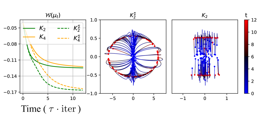
Figure 1: (Left) Value of $\mathcal{W}$ along the flow for two difference interaction Bregman potentials, (Middle and Right) Trajectories of particles to minimize $\mathcal{W}$.

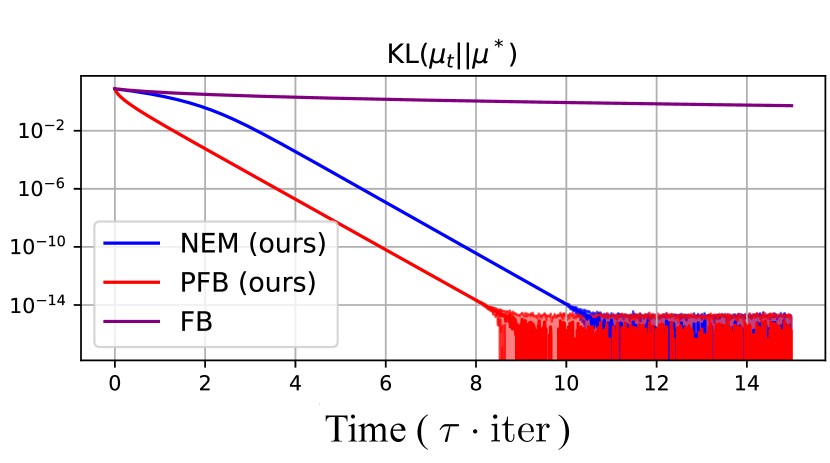
Figure 2: Convergence towards Gaussians $\mathcal{N}(0,UDU^{T})$ averaged over 20 covariances, with $U\sim\mathrm{Unif}(O_{10}(\mathbb{R}))$ and $D$ fixed.

MD on interaction energies.

We first focus on minimizing interaction energies $\mathcal{W}$ with kernel $W(z)=\frac{1}{4}\|z\|_{\Sigma^{-1}}^{4}-\frac{1}{2}\|z\|_{\Sigma^{-1}}^{2}$ with $\Sigma\in S_{d}^{++}(\mathbb{R})$, whose minimizer is an ellipsoid [26]. Since its Hessian norm can be bounded by a polynomial of degree 2, following [81, Section 2], $W$ is smooth relative to $K_{4}(z)=\frac{1}{4}\|z\|_{2}^{4}+\frac{1}{2}\|z\|_{2}^{2}$ and $\mathcal{W}$ is smooth relative to $\phi_{\mu}(\mathrm{T})=\iint K_{4}\big{(}\mathrm{T}(x)-\mathrm{T}(y)\big{)}\ \mathrm{d}\mu(x)\mathrm{d}\mu(y)$. Supposing additionally that the distributions are compactly supported, we can show that $\mathcal{W}$ is smooth relative to the interaction energy with $K_{2}(z)=\frac{1}{2}\|z\|_{2}^{2}$. For ill-conditioned $\Sigma$, the convergence can be slow. Thus, we also propose to use $K_{2}^{\Sigma}(z)=\frac{1}{2}\|z\|_{\Sigma^{-1}}^{2}$ and $K_{4}^{\Sigma}(z)=\frac{1}{4}\|z\|_{\Sigma^{-1}}^{4}+\frac{1}{2}\|z\|_{\Sigma^{-1}}^{2}$. We illustrate these schemes on Figure 2 and observe the convergence we expect for the schemes taking into account $\Sigma$. In practice, since $\nabla\phi_{\mu}(\mathrm{T})=(\nabla K\star\mathrm{T}_{\#}\mu)\circ\mathrm{T}$, the scheme needs to be approximated using Newton’s algorithm which can be computationally heavy. Using $\phi_{\mu}^{V}(\mathrm{T})=\int V\circ\mathrm{T}\ \mathrm{d}\mu$ with $V=K_{2}^{\Sigma}$, we obtain a more computationally friendly scheme with the same convergence, see Section G.2, but for which the smoothness is trickier to show.

MD on KL.

We now focus on minimizing $\mathcal{F}(\mu)=\int V\mathrm{d}\mu+\mathcal{H}(\mu)$ for $V(x)=\frac{1}{2}x^{T}\Sigma^{-1}x$ with $\Sigma$ possibly ill-conditioned, whose minimizer is the Gaussian $\nu=\mathcal{N}(0,\Sigma)$, and for which $\mathrm{W}_{2}$-gradient descent is slow to converge. We study the MD scheme in (4) with negative entropy $\mathcal{H}$ as the Bregman potential (NEM), and compare it on Figure 2 with the Forward-Backward (FB) scheme studied in [40] and the ideally preconditioned Forward-Backward scheme (PFB) with Bregman potential $\phi_{\mu}^{V}$ (see (115) in Appendix F). For computational purpose, we restrain the minimization in (4) over affine maps, which can be seen as taking the gradient over the submanifold of Gaussians [68, 40]. Starting from $\mathcal{N}(0,\Sigma_{0})$, the distributions stay Gaussian over the flow, and their closed-form is reported in (63) (Section D.3). We note that this might not be the case for the scheme (4), and thus that this scheme does not enter into the framework developed in the previous sections. Nonetheless, it demonstrates the benefits of using different Bregman potentials. We generate 20 Gaussian targets $\nu$ on $\mathbb{R}^{10}$ with $\Sigma=UDU^{T}$, $D$ diagonal and scaled in log space between 1 and 100, and $U$ a uniformly sampled orthogonal matrices, and we report the averaged KL over time. Surprisingly, NEM, which does not require an ideal (and not available in general) preconditioner, is almost as fast to converge as the ideal PFB, and much faster than the FB scheme.

Figure 3: Preconditioned GD vs. (vanilla) GD to predict the responses of cell populations to cancer treatment on 4i (Upper row) and scRNAseq (Lower row) datasets. For each treatment, starting from the untreated cells $\mu_{i}$, we minimize $\mathcal{F}(\mu)=D(\mu,\nu_{i})$ with $\nu_{i}$ the treated cells. The plot is organized as pairs of columns, each corresponding to optimizing a specific metric, with two scatter plots displaying points $z_{i}=(x_{i},y_{i})$ where (First column) $y_{i}$ is the attained minima $\mathcal{F}(\hat{\mu})=D(\hat{\mu},\nu_{i})$ with preconditioning and $x_{i}$ that without preconditioning, and (Second column) $y_{i}$ is the number of iterations to reach convergence with preconditioning and $x_{i}$ that without preconditioning. A point below the diagonal $y=x$ then refers to an experiment in which preconditioning provides (First column) a better minima or (Second column) faster convergence. We assign a color to each treatment and plot three runs, obtained with three different initializations, along with their mean (brighter point).

Preconditioned GD for single-cells.

Predicting the response of cells to a perturbation is a central question in biology. In this context, as the measuring process is destructive, feature descriptions of control and treated cells must be dealt with as (unpaired) source $\mu$ and target distributions $\nu$. Following [104], OT theory to recover a mapping $T$ between these two populations has been used in [20, 22, 21, 36, 45, 112, 64]. Inspired by the recent success of iterative refinement in generative modeling, through diffusion [57, 107] or flow-based models [78, 74], our scheme (1) follows the idea of transporting $\mu$ to $\nu$ via successive and dynamic displacements instead of, directly, with a static map $\bar{T}$. We model the transition from unperturbed to perturbed states through the (preconditioned) gradient flow of a functional $\mathcal{F}(\mu)=D(\mu,\nu)$ initialized at $\mu_{0}=\mu$, where $D$ is a distributional metric, and predict the perturbed population via $\hat{\mu}=\min_{\mu}\mathcal{F}(\mu)$. We focus on the datasets used in [20], consisting of cell lines analyzed using (i) 4i [54], and (ii) scRNA sequencing [110]. For each profiling technology, the response to respectively (i) 34 and (ii) 9 treatments are provided. As in [20], training is performed in data space for the 4i data and in a latent space learned by the scGen autoencoder [80] for the scRNA data. We use three metrics: the Sliced-Wasserstein distance $\mathrm{SW}_{2}^{2}$ [16], the Sinkhorn divergence $\mathrm{S}_{\varepsilon,2}^{2}$ [47] and the energy distance $\mathrm{ED}$ [98, 56, 55], and we compare the performances when minimizing this functional via preconditioned GD vs. (vanilla) GD. We measure the convergence speed when using a fixed relative tolerance $\textrm{tol}=10^{-3}$, as well as the attained optimal value $\mathcal{F}(\hat{\mu})$. Note that we follow [20] and additionally consider 40% of unseen (test) target cells for evaluation, i.e., for computing $\mathcal{F}(\hat{\mu})=D(\hat{\mu},\nu)$. As preconditioner, we use the one induced by $h^{*}(\*x)=(\|x\|_{2}^{a}+1)^{1/a}-1$ with $a>0$, which is well suited to minimize functionals which grow in $\|x-x^{*}\|^{a/(a-1)}$ near their minimum [111]. We set the step size $\tau=1$ for all the experiments. Then, we tune $a$ very simply: for a given metric $D$ and a profiling technology, we pick a random treatment and select $a\in\{1.25,1.5,1.75\}$ by grid search, and we generalize the selected $a$ for all the other treatments. Results are described in Figure 3: Preconditioned GD significantly outperforms GD over the 43 datasets, in terms of convergence speed and optimal value $\mathcal{F}(\hat{\mu})$. For instance, for $D=\mathrm{S}_{2,\varepsilon}^{2}$, we converge in 10 times less iterations while providing, on average, a better estimate of the treated population. We also compare our iterative (non parametric) approach with the use of a static (non parametric) map in Section G.4.

6 Conclusion

In this work, we extended two non-Euclidean optimization methods on $\mathbb{R}^{d}$ to the Wasserstein space, generalizing $\mathrm{W}_{2}$-gradient descent to alternative geometries. We investigated the practical benefits of these schemes, and provided rates of convergences for pairs of objectives and Bregman potentials satisfying assumptions of relative smoothness and convexity along specific curves. While these assumptions can be easily checked is some cases (e.g. potential or interaction energies) by comparing the Bregman divergences or Hessian operators in the Wasserstein geometry, they may be hard to verify in general. Different objectives such as the Sliced-Wasserstein distance or the Sinkhorn divergence, or alternative geometries to the Wasserstein-2 as studied in this work, require to derive specific computations on a case-by-case basis. We leave this investigation for future work.

Appendix

Contents

1. 1 Introduction
2. 2 Background
3. 3 Mirror descent
4. 4 Preconditioned gradient descent
5. 5 Applications and Experiments
6. 6 Conclusion
7. A Related works
8. B Background on $L^{2}(\mu)$
   1. B.1 Differential calculus on $L^{2}(\mu)$
   2. B.2 Convexity on $L^{2}(\mu)$
9. C Background on Wasserstein space
   1. C.1 Wasserstein differentials
   2. C.2 Wasserstein Hessians
   3. C.3 Convexity in Wasserstein space
10. D Additional results on mirror descent
    1. D.1 Optimal transport maps for mirror descent
    2. D.2 Continuous formulation
    3. D.3 Derivation in specific settings
    4. D.4 Mirror scheme with non-pushforward compatible Bregman potentials
11. E Relative convexity and smoothness
    1. E.1 Relative convexity and smoothness between Fenchel transforms
    2. E.2 Relative convexity and smoothness between functionals
12. F Bregman proximal gradient scheme
13. G Additional details on experiments
    1. G.1 Solving the general scheme
    2. G.2 Mirror descent of interaction energies
    3. G.3 Mirror descent on Gaussians
    4. G.4 Single-cell experiments
    5. G.5 Mirror descent on the simplex
14. H Proofs
    1. H.1 Proof of Proposition 1
    2. H.2 Proof of Proposition 2
    3. H.3 Proof of Proposition 3
    4. H.4 Proof of Proposition 4
    5. H.5 Proof of Proposition 5
    6. H.6 Proof of Lemma 9
    7. H.7 Proof of Proposition 10
    8. H.8 Proof of Proposition 11
    9. H.9 Proof of Proposition 22
    10. H.10 Proof of Proposition 23
    11. H.11 Proof of Lemma 24
    12. H.12 Proof of Proposition 25
15. I Additional results
    1. I.1 Three-point identity and inequality
    2. I.2 Convergence lemma
    3. I.3 Some properties of Bregman divergences

Appendix A Related works

Wasserstein Gradient flows with respect to non-Euclidean geometries. Several existing schemes are based on time-discretizations of gradient flows with respect to optimal transport metrics, but different than the Wasserstein-2 distance.

To simplify the computation of the backward scheme, Peyré [93] added an entropic regularization into the JKO scheme while Bonet et al. [14] considered using the Sliced-Wasserstein distance instead. More recently, Rankin and Wong [97] suggested using Bregman divergences e.g. when geodesic distances are not known in closed-forms.

The most popular objective in Wasserstein gradient flows is the KL. However, this can be intricate to compute as it requires the evaluation of the density at each step, which is not known for particles, and thus requires approximations using kernel density estimators [116] or density ratio estimators [5, 117, 46]. Restricting the velocity field to a reproducing kernel Hilbert space (RKHS), an update in closed-form can be obtained, which is given by the SVGD algorithm [77, 76]. This algorithm can also be seen as using an alternative Wasserstein metric [43]. However, the restriction to RKHS can hinder the flexibility of the method. This motivated the introduction of new schemes based on using the Wasserstein distance with a convex translation invariant cost [41, 29]. Particle systems preconditioned by they empirical covariance matrix have also been recently considered, and can be seen as discretization of the Kalman-Wasserstein or Covariance Modulated gradient flow [52, 23].

Mirror descent with flat geometry.

The space of probability distributions can be endowed with different metrics. When endowed with the Fisher-Rao metric instead of the Wasserstein distance, the geometry becomes very different. Notably, the shortest path between the two distributions is now a mixture between them. In this situation, the gradient is the first variation. Aubin-Frankowski et al. [8] studied the mirror descent in this space and notably showed connections with Sinkhorn algorithm when the mirror map and the optimized function are KL divergences. Karimi et al. [62] extended the mirror descent algorithm for more general time steps, and notably recovered the “Wasserstein Mirror Flow” proposed by Deb et al. [38] as a special case.

Bregman divergence on $\mathcal{P}_{2}(\mathbb{R}^{d})$.

Several works introduced Bregman divergences on $\mathcal{P}_{2}(\mathbb{R}^{d})$. Carlier and Jimenez [24] first studied the existence of Monge maps for the OT problem with Bregman costs $c(x,y)=\mathrm{d}_{V}(x,y)$ and symmetrized Bregman costs $c(x,y)=\mathrm{d}_{V}(x,y)+\mathrm{d}_{V}(y,x)$. For Bregman costs, the resulting OT problem was named the Bregman-Wasserstein divergence and its properties were studied in [53, 34, 96]. The Bregman-Wasserstein divergence has also been used by Ahn and Chewi [3] to show the convergence of the Mirror Langevin algorithm while Rankin and Wong [97] studied its JKO scheme with KL objective. Li [73] introduced the notion of Bregman divergence on Wasserstein space for a geodesically strictly convex $\mathcal{F}:\mathcal{P}_{2}(\mathbb{R}^{d})\to\mathbb{R}$ as

$$\forall\mu,\nu\in\mathcal{P}_{2}(\mathbb{R}^{d}),\ \mathrm{d}_{\mathcal{F}}(\mu,\nu)=\mathcal{F}(\mu)-\mathcal{F}(\nu)-\langle\nabla_{\mathrm{W}_{2}}\mathcal{F}(\nu),\mathrm{T}_{\nu}^{\mu}-\mathrm{Id}\rangle_{L^{2}(\nu)},$$ (14)

where $\mathrm{T}_{\nu}^{\mu}$ is the OT map between $\nu$ and $\mu$ w.r.t $\mathrm{W}_{2}$. The Bregman divergence used in our work and as defined in Definition 1 is more general as it allows using more general maps and contains as special case (14). Li [73] studied properties of this Bregman divergence for different functionals $\mathcal{F}$ and provided closed-forms for one-dimensional distributions or Gaussian, but did not use it to define a mirror scheme.

Mirror descent on $\mathcal{P}_{2}(\mathbb{R}^{d})$.

Deb et al. [38] defined a mirror flow by using the continuous formulation. They focused on KL objectives with Bregman potential $\phi(\mu)=\frac{1}{2}\mathrm{W}_{2}^{2}(\mu,\nu)$ with some reference measure $\nu\in\mathcal{P}_{2}(\mathbb{R}^{d})$, and defined the flow as the solution of

$$\begin{cases}\varphi(\mu_{t})=\nabla_{\mathrm{W}_{2}}\phi(\mu_{t})\\ \frac{\mathrm{d}}{\mathrm{d}t}\varphi(\mu_{t})=-\nabla_{\mathrm{W}_{2}}\mathcal{F}(\mu_{t}).\end{cases}$$ (15)

We note that $\phi$ is pushforward compatible and hence enters our framework. Also related to our work, Wang and Li [115] studied a Wasserstein Newton’s flow, which, analogously to the relation between Newton’s method and mirror descent [30], is another discretization of our scheme for $\phi=\mathcal{F}$. We clarify the link with the Mirror Descent algorithm we define in this work with the previous continuous formulation above in Section D.2.

Appendix B Background on $L^{2}(\mu)$

B.1 Differential calculus on $L^{2}(\mu)$

We recall some differentiability definitions on the Hilbert space $L^{2}(\mu)$ for $\mu\in\mathcal{P}_{2}(\mathbb{R}^{d})$. Let $\phi:L^{2}(\mu)\to\mathbb{R}$. We start by recalling the notions of Gâteaux and Fréchet derivatives.

Definition 4.

A function $\phi:L^{2}(\mu)\to\mathbb{R}$ is said to be Gâteaux differentiable at $T$ if there exists an operator $\phi^{\prime}(\mathrm{T}):L^{2}(\mu)\to\mathbb{R}$ such that for any direction $h\in L^{2}(\mu)$,

$$\phi^{\prime}(\mathrm{T})(h)=\lim_{t\to 0}\ \frac{\phi(\mathrm{T}+th)-\phi(\mathrm{T})}{t},$$ (16)

and $\phi^{\prime}(\mathrm{T})$ is a linear function. The operator $\phi^{\prime}(\mathrm{T})$ is called the Gâteaux derivative of $\phi$ at $\mathrm{T}$ and if it exists, it is unique.

Definition 5.

The Fréchet derivative of $\phi$ denoted $\delta\phi$ is defined implicitly by

$$\phi(\mathrm{T}+th)=\phi(\mathrm{T})+t\delta\phi(\mathrm{T},h)+to(\|h\|).$$ (17)

If $\phi$ is Fréchet differentiable, then it is also Gâteaux differentiable, and both derivatives agree, i.e. for all $\mathrm{T},h\in L^{2}(\mu)$, $\delta\phi(\mathrm{T},h)=\phi^{\prime}(\mathrm{T})(h)$ [92, Proposition 1.26].

Moreover, since $L^{2}(\mu)$ is a Hilbert space, and $\delta\phi(\mathrm{T},\cdot)$ and $\phi^{\prime}(\mathrm{T})$ are linear and continuous, if $\phi$ is Fréchet (resp. Gâteaux) differentiable, by the Riesz representation theorem, there exists $\nabla\phi\in L^{2}(\mu)$ such that for all $h\in L^{2}(\mu)$, $\delta\phi(\mathrm{T},h)=\langle\nabla\phi(\mathrm{T}),h\rangle_{L^{2}(\mu)}$ (resp. $\phi^{\prime}(\mathrm{T})(h)=\langle\nabla\phi(\mathrm{T}),h\rangle_{L^{2}(\mu)}$).

As a brief comment on these notions in the context of convexity, if the subdifferential of a convex $f$ at $x$ contains a single element then it is the Gâteaux derivative and we have an inequality $f(y)\geq f(x)+\langle\nabla f(x),y-x\rangle$. Instead Fréchet différentiability gives an equality (17) corresponding to a series expansion.

B.2 Convexity on $L^{2}(\mu)$

Let $\phi:L^{2}(\mu)\to\mathbb{R}$ be Gâteaux differentiable. We recall that $\phi$ is convex if for all $t\in[0,1]$, $\mathrm{T},\mathrm{S}\in L^{2}(\mu)$,

$$\phi\big{(}(1-t)\mathrm{T}+t\mathrm{S}\big{)}\leq(1-t)\phi(\mathrm{T})+t\phi(\mathrm{S}),$$ (18)

which is equivalent by [92, Proposition 3.10] with

$$\forall\mathrm{T},\mathrm{S}\in L^{2}(\mu),\ \phi(\mathrm{T})\geq\phi(\mathrm{S})+\langle\nabla\phi(\mathrm{S}),\mathrm{T}-\mathrm{S})\rangle_{L^{2}(\mu)}\iff\mathrm{d}_{\phi}(\mathrm{T},\mathrm{S})\geq 0.$$ (19)

We now present equivalent definitions of the relative smoothness and relative convexity, which is the equivalent of [81, Proposition 1.1].

Proposition 6.

Let $\psi,\phi:L^{2}(\mu)\to\mathbb{R}$ be convex and Gâteaux differentiable functions. The following conditions are equivalent:

1. $\psi$ $\beta$-smooth relative to $\phi$

2. $\beta\phi-\psi$ convex

3. If twice Gâteaux differentiable, $\langle\nabla^{2}\psi(\mathrm{T})\mathrm{S},\mathrm{S}\rangle_{L^{2}(\mu)}\leq\beta\langle\nabla^{2}\phi(\mathrm{T})\mathrm{S},\mathrm{S}\rangle_{L^{2}(\mu)}$ for all $\mathrm{T},\mathrm{S}\in L^{2}(\mu)$

4. $\langle\nabla\psi(\mathrm{T})-\nabla\psi(\mathrm{S}),\mathrm{T}-\mathrm{S}\rangle_{L^{2}(\mu)}\leq\beta\langle\nabla\phi(\mathrm{T})-\nabla\phi(\mathrm{S}),\mathrm{T}-\mathrm{S}\rangle_{L^{2}(\mu)}$ for all $\mathrm{T},\mathrm{S}\in L^{2}(\mu)$.

The following conditions are equivalent:

1. $\psi$ $\alpha$-convex relative to $\phi$

2. $\psi-\alpha\phi$ convex

3. If twice differentiable, $\langle\nabla^{2}\psi(\mathrm{T})\mathrm{S},\mathrm{S}\rangle_{L^{2}(\mu)}\geq\alpha\langle\nabla^{2}\phi(\mathrm{T})\mathrm{S},\mathrm{S}\rangle_{L^{2}(\mu)}$ for all $\mathrm{T},\mathrm{S}\in L^{2}(\mu)$

4. $\langle\nabla\psi(\mathrm{T})-\nabla\psi(\mathrm{S}),\mathrm{T}-\mathrm{S}\rangle_{L^{2}(\mu)}\geq\alpha\langle\nabla\phi(\mathrm{T})-\nabla\phi(\mathrm{S}),\mathrm{T}-\mathrm{S}\rangle_{L^{2}(\mu)}$ for all $\mathrm{T},\mathrm{S}\in L^{2}(\mu)$.

Proof.

We do it only for the smoothness. It holds likewise for the convexity.

(a1)$\iff$(a2):

$$\forall\mathrm{T},\mathrm{S}\in L^{2}(\mu),\ \mathrm{d}_{\psi}(\mathrm{T},\mathrm{S})\leq\beta\mathrm{d}_{\phi}(\mathrm{T},\mathrm{S})$$ (20)

$$\iff\forall\mathrm{T},\mathrm{S}\in L^{2}(\mu),\ \psi(\mathrm{T})-\psi(\mathrm{S})-\langle\nabla\psi(\mathrm{S}),\mathrm{T}-\mathrm{S}\rangle_{L^{2}(\mu)}$$

$$\qquad\qquad\qquad\qquad\qquad\qquad\qquad\leq\beta\big{(}\phi(\mathrm{T})-\phi(\mathrm{S})-\langle\nabla\phi(\mathrm{S}),\mathrm{T}-\mathrm{S}\rangle_{L^{2}(\mu)}\big{)}$$

$$\iff\forall\mathrm{T},\mathrm{S}\in L^{2}(\mu),\ (\beta\phi-\psi)(\mathrm{S})-\langle\nabla(\beta\phi-\psi)(\mathrm{S}),\mathrm{T}-\mathrm{S}\rangle_{L^{2}(\mu)}\leq(\beta\phi-\psi)(\mathrm{T}).$$

For the rest of the equivalences, we apply [92, Proposition 3.10]. Indeed, $\beta\phi-\psi$ convex is equivalent with

$$\forall\mathrm{T},\mathrm{S}\in L^{2}(\mu),\ \langle\nabla(\beta\phi-\psi)(\mathrm{T})-\nabla(\beta\phi-\psi)(\mathrm{S}),\mathrm{T}-\mathrm{S}\rangle_{L^{2}(\mu)}\geq 0\\ \iff\forall\mathrm{T},\mathrm{S}\in L^{2}(\mu),\ \beta\langle\phi(\mathrm{T})-\nabla\phi(\mathrm{S}),\mathrm{T}-\mathrm{S}\rangle_{L^{2}(\mu)}\geq\langle\nabla\psi(\mathrm{T})-\nabla\psi(\mathrm{S}),\mathrm{T}-\mathrm{S}\rangle_{L^{2}(\mu)},$$ (21)

which gives the equivalence between (a2) and (a4). And if $\psi$ and $\phi$ are twice differentiables, it is also equivalent with

$$\forall\mathrm{T},\mathrm{S}\in L^{2}(\mu),\ \langle\nabla^{2}(\beta\phi-\psi)(\mathrm{T})\mathrm{S},\mathrm{S}\rangle_{L^{2}(\mu)}\geq 0\\ \iff\forall\mathrm{T},\mathrm{S}\in L^{2}(\mu),\ \beta\langle\nabla^{2}\phi(\mathrm{T})\mathrm{S},\mathrm{S}\rangle_{L^{2}(\mu)}\geq\langle\psi(\mathrm{T})\mathrm{S},\mathrm{S}\rangle_{L^{2}(\mu)},$$ (22)

which gives the equivalence between (a2) and (a3). ∎

Appendix C Background on Wasserstein space

C.1 Wasserstein differentials

We recall the notion of Wasserstein differentiability introduced in [17, 69]. First, we introduce sub and super differential.

Definition 6 (Wasserstein sub- and super-differential [17, 69]).

Let $\mathcal{F}:\mathcal{P}_{2}(\mathbb{R}^{d})\to(-\infty,+\infty]$ lower semi-continuous and denote $D(\mathcal{F})=\{\mu\in\mathcal{P}_{2}(\mathbb{R}^{d}),\ \mathcal{F}(\mu)<\infty\}$. Let $\mu\in D(\mathcal{F})$. Then, a map $\xi\in L^{2}(\mu)$ belongs to the subdifferential $\partial^{-}\mathcal{F}(\mu)$ of $\mathcal{F}$ at $\mu$ if for all $\nu\in\mathcal{P}_{2}(\mathbb{R}^{d})$,

$$\mathcal{F}(\nu)\geq\mathcal{F}(\mu)+\sup_{\gamma\in\Pi_{o}(\mu,\nu)}\int\langle\xi(x),y-x\rangle\ \mathrm{d}\gamma(x,y)+o\big{(}\mathrm{W}_{2}(\mu,\nu)\big{)}.$$ (23)

Similarly, $\xi\in L^{2}(\mu)$ belongs to the superdifferential $\partial^{+}\mathcal{F}(\mu)$ of $\mathcal{F}$ at $\mu$ if $-\xi\in\partial^{-}(-\mathcal{F})(\mu)$.

Then, we say that a functional is Wasserstein differentiable if it admits sub and super differentials which coincide.

Definition 7 (Wasserstein differentiability, Definition 2.3 in [69]).

A functional $\mathcal{F}:\mathcal{P}_{2}(\mathbb{R}^{d})\to\mathbb{R}$ is Wasserstein differentiable at $\mu\in\mathcal{P}_{2}(\mathbb{R}^{d})$ if $\partial^{-}\mathcal{F}(\mu)\cap\partial^{+}\mathcal{F}(\mu)\neq\emptyset$. In this case, we say that $\nabla_{\mathrm{W}_{2}}\mathcal{F}(\mu)\in\partial^{-}\mathcal{F}(\mu)\cap\partial^{+}\mathcal{F}(\mu)$ is a Wasserstein gradient of $\mathcal{F}$ at $\mu$, satisfying for any $\nu\in\mathcal{P}_{2}(\mathbb{R}^{d})$, $\gamma\in\Pi_{o}(\mu,\nu)$,

$$\mathcal{F}(\nu)=\mathcal{F}(\mu)+\int\langle\nabla_{\mathrm{W}_{2}}\mathcal{F}(\mu)(x),y-x\rangle\ \mathrm{d}\gamma(x,y)+o\big{(}\mathrm{W}_{2}(\mu,\nu)\big{)}.$$ (24)

Recall that the tangent space of $\mathcal{P}_{2}(\mathbb{R}^{d})$ at $\mu\in\mathcal{P}_{2}(\mathbb{R}^{d})$ is defined as

$$\mathcal{T}_{\mu}\mathcal{P}_{2}(\mathbb{R}^{d})=\overline{\left\{\nabla\psi,\;\psi\in\mathcal{C}_{c}^{\infty}(\mathbb{R}^{d})\right\}}\subset L^{2}(\mu),$$

where the closure is taken in $L^{2}(\mu)$, see Ambrosio et al. [4, Definition 8.4.1]. Lanzetti et al. [69, Proposition 2.5] showed that if $\mathcal{F}$ is Wasserstein differentiable, then there is always a unique gradient living in the tangent space, and we can restrict ourselves without loss of generality to this gradient.

Lanzetti et al. [69] further showed that Wasserstein gradients provide linear approximations even if the perturbations are not induced by OT plans, i.e. differentials are “strong Fréchet differentials”.

Proposition 7 (Proposition 2.6 in [69]).

Let $\mu,\nu\in\mathcal{P}_{2}(\mathbb{R}^{d})$, $\gamma\in\Pi(\mu,\nu)$ any coupling and let $\mathcal{F}:\mathcal{P}_{2}(\mathbb{R}^{d})\to\mathbb{R}$ be Wasserstein differentiable at $\mu$ with Wasserstein gradient $\nabla_{\mathrm{W}_{2}}\mathcal{F}(\mu)\in\mathcal{T}_{\mu}\mathcal{P}_{2}(\mathbb{R}^{d})$. Then,

$$\mathcal{F}(\nu)=\mathcal{F}(\mu)+\int\langle\nabla_{\mathrm{W}_{2}}\mathcal{F}(\mu)(x),y-x\rangle\ \mathrm{d}\gamma(x,y)+o\left(\sqrt{\int\|x-y\|_{2}^{2}\ \mathrm{d}\gamma(x,y)}\right).$$ (25)

The Wasserstein gradient of $\mathcal{F}$ can be computed in practice using the first variation $\frac{\delta\mathcal{F}}{\delta\mu}$ [102, Definition 7.12], which is defined, if is exists, as the unique function (up to a constant) such that, for $\chi$ satisfying $\int\mathrm{d}\chi=0$,

$$\frac{\mathrm{d}}{\mathrm{d}t}\mathcal{F}(\mu+t\chi)\Big{|}_{t=0}=\lim_{t\to 0}\ \frac{\mathcal{F}(\mu+t\chi)-\mathcal{F}(\mu)}{t}=\int\frac{\delta\mathcal{F}}{\delta\mu}(\mu)\ \mathrm{d}\chi.$$ (26)

Then the Wasserstein gradient can be computed as $\nabla_{\mathrm{W}_{2}}\mathcal{F}(\mu)=\nabla\frac{\delta\mathcal{F}}{\delta\mu}(\mu)$.

We now show that we can relate the Fréchet derivative of $\tilde{\mathcal{F}}_{\mu}(\mathrm{T}):=\mathcal{F}(\mathrm{T}_{\#}\mu)$ with the Wasserstein gradient of $\mathcal{F}$ belonging to the tangent space of $\mathcal{P}_{2}(\mathbb{R}^{d})$ at $\mu$.

Proposition 8.

Let $\mathcal{F}:\mathcal{P}_{2}(\mathbb{R}^{d})\to\mathbb{R}\cup\{+\infty\}$ be a Wasserstein differentiable functional on $D(\mathcal{F})$. Let $\mu\in\mathcal{P}_{2}(\mathbb{R}^{d})$ and $\tilde{\mathcal{F}}_{\mu}(\mathrm{T})=\mathcal{F}(\mathrm{T}_{\#}\mu)$ for all $\mathrm{T}\in D(\tilde{\mathcal{F}}_{\mu})$. Then, $\tilde{\mathcal{F}}_{\mu}$ is Fréchet differentiable, and for all $\mathrm{S}\in D(\tilde{\mathcal{F}}_{\mu})$, $\nabla\tilde{\mathcal{F}}_{\mu}(\mathrm{S})=\nabla_{\mathrm{W}_{2}}\mathcal{F}(\mathrm{S}_{\#}\mu)\circ\mathrm{S}$.

Proof.

Let $\mu\in\mathcal{P}_{2}(\mathbb{R}^{d})$, $\mathrm{S},\mathrm{T}\in D(\tilde{\mathcal{F}}_{\mu})$, $\epsilon>0$. Since $\mathcal{F}$ is Wasserstein differentiable at $\mathrm{S}_{\#}\mu$, applying Proposition 7 at $\mathrm{S}_{\#}\mu$ with $\nu=\big{(}\mathrm{S}+\epsilon(\mathrm{T}-\mathrm{S})\big{)}_{\#}\mu$ and $\gamma=\big{(}\mathrm{S},\mathrm{S}+\epsilon(\mathrm{T}-\mathrm{S})\big{)}_{\#}\mu\in\Pi(\mathrm{S}_{\#}\mu,\nu)$, we obtain,

$$\tilde{\mathcal{F}}_{\mu}\big{(}\mathrm{S}+\epsilon(\mathrm{T}-\mathrm{S})\big{)} =\mathcal{F}\big{(}(\mathrm{S}+\epsilon(\mathrm{T}-\mathrm{S}))_{\#}\mu\big{)}$$

$$=\mathcal{F}(\mathrm{S}_{\#}\mu)+\int\langle\nabla_{\mathrm{W}_{2}}\mathcal{F}(\mathrm{S}_{\#}\mu)(x),y-x\rangle\ \mathrm{d}\gamma(x,y)$$

$$\quad+o\left(\sqrt{\int\|x-y\|_{2}^{2}\ \mathrm{d}\gamma(x,y)}\right)$$

$$=\tilde{\mathcal{F}}_{\mu}(\mathrm{S})+\epsilon\int\langle\nabla_{\mathrm{W}_{2}}\mathcal{F}(\mathrm{S}_{\#}\mu)\big{(}\mathrm{S}(x)\big{)},\mathrm{T}(x)-\mathrm{S}(x)\rangle\ \mathrm{d}\mu(x)$$

$$\quad+o\left(\epsilon\sqrt{\int\|\mathrm{T}(x)-\mathrm{S}(x)\|_{2}^{2}\ \mathrm{d}\mu(x)}\right)$$

$$=\tilde{\mathcal{F}}_{\mu}(\mathrm{S})+\epsilon\langle\nabla_{\mathrm{W}_{2}}\mathcal{F}(\mathrm{S}_{\#}\mu)\circ\mathrm{S},\mathrm{T}-\mathrm{S}\rangle_{L^{2}(\mu)}+\epsilon o(\|\mathrm{T}-\mathrm{S}\|_{L^{2}(\mu)}).$$ (27)

Thus, $\delta\tilde{\mathcal{F}}_{\mu}(\mathrm{S},\mathrm{T}-\mathrm{S})=\langle\nabla_{\mathrm{W}_{2}}\mathcal{F}(\mathrm{S}_{\#}\mu)\circ\mathrm{S},\mathrm{T}-\mathrm{S}\rangle_{L^{2}(\mu)}$. Note that in the third equality we used that $\nabla_{\mathrm{W}_{2}}\mathcal{F}\in L^{2}(\mu)$. ∎

A similar formula can be found in Gangbo and Tudorascu [51, Corollary 3.22], however the space $H$ used there is not $L^{2}(\mu)$ but a lifting $L^{2}(\Omega;\mathbb{R}^{d})$ of measures on random variables. They should not be confused.

C.2 Wasserstein Hessians

A natural object of interest is the Hessian of the objective $\mathcal{F}$, which we define below. This notion is usually defined along Wasserstein geodesics, i.e. curves of the form $\mu_{t}=(\mathrm{Id}+t\nabla\psi)_{\#}\mu$ for $\psi\in\mathcal{C}_{c}^{\infty}(\mathbb{R}^{d})$ [67].

Definition 8.

The Wasserstein Hessian of a functional $\mathcal{F}:\mathcal{P}_{2}(\mathbb{R}^{d})\to\mathbb{R}$ at $\mu$ is defined for any $\psi\in\mathcal{C}_{c}^{\infty}(\mathbb{R}^{d})$ as:

$$\operatorname{Hess}_{\mu}\mathcal{F}(\psi,\psi):=\derivative[2]{t}\mathcal{\mathcal{F}}(\mu_{t})\big{|}_{t=0}$$

where $(\mu_{t},v_{t})_{t\in[0,1]}$ is a Wasserstein geodesic with $\mu_{0}=0,v_{0}=\nabla\psi$.

Definition 8 can be straightforwardly related to the usual symmetric bilinear form defined on $\mathcal{T}_{\mu}\mathcal{P}_{2}(\mathbb{R}^{d})\times\mathcal{T}_{\mu}\mathcal{P}_{2}(\mathbb{R}^{d})$ [90, Section 3]:

Definition 9.

The Wasserstein Hessian of $\mathcal{F}$, denoted $\mathrm{H}\mathcal{F}_{\mu}$ is an operator over $\mathcal{T}_{\mu}\mathcal{P}_{2}(\mathbb{R}^{d})$ verifying $\langle\mathrm{H}\mathcal{F}_{\mu}v_{0},v_{0}\rangle_{L^{2}(\mu)}=\frac{\mathrm{d}^{2}}{\mathrm{d}t^{2}}\mathcal{F}(\rho_{t})\big{|}_{t=0}$ if $(\rho_{t},v_{t})_{t\in[0,1]}$ is a Wasserstein geodesic starting at $\mu$.

In this work, we are interested in more general curves, which are acceleration free, i.e. of the form $\mu_{t}=(\mathrm{S}+tv)_{\#}\mu$ with $\mathrm{S},v\in L^{2}(\mu)$. Thus, we define analogously the Hessian and the Hessian operator along such curves. We note that if $\mathrm{S}$ is invertible, $\mu_{t}=(\mathrm{Id}+tv\circ\mathrm{S}^{-1})_{\#}\mathrm{S}_{\#}\mu$, and the notions can be linked with Wasserstein Hessian. However, in general, this does not need to be the case.

Definition 10.

The Hessian of $\mathcal{F}:\mathcal{P}_{2}(\mathbb{R}^{d})\to\mathbb{R}$ along $t\mapsto\mu_{t}=(\mathrm{S}+tv)_{\#}\mu$ for $\mathrm{S},v\in L^{2}(\mu)$ is defined as

$$\operatorname{Hess}_{\mu,t}\mathcal{F}(v,v)=\frac{\mathrm{d}^{2}}{\mathrm{d}t^{2}}\mathcal{F}(\mu_{t}).$$ (28)

Moreover, we define the Hessian operator $\mathrm{H}\mathcal{F}_{\mu,t}:L^{2}(\mu)\to L^{2}(\mu)$ as the operator satisfying for all $t\in[0,1]$,

$$\frac{\mathrm{d}^{2}}{\mathrm{d}t^{2}}\mathcal{F}(\mu_{t})=\langle\mathrm{H}\mathcal{F}_{\mu,t}v,v\rangle_{L^{2}(\mu)}.$$ (29)

Wang and Li [115] derived a general closed form of the Wasserstein Hessian through the first variation of $\mathcal{F}$. Here, we extend their formula along any curve $\mu_{t}=(\mathrm{S}+tv)_{\#}\mu$ with $\mathrm{S},v\in L^{2}(\mu)$. We first provide a lemma computing the derivative of the Wasserstein gradient.

Lemma 9.

Let $\mathcal{F}:\mathcal{P}_{2}(\mathbb{R}^{d})\to\mathbb{R}$ be twice continuously differentiable and assume that $\frac{\delta}{\delta\mu}\nabla\frac{\delta\mathcal{F}}{\delta\mu}=\nabla\frac{\delta^{2}\mathcal{F}}{\delta\mu^{2}}$. Let $\mu\in\mathcal{P}_{2}(\mathbb{R}^{d})$ and for all $t\in[0,1]$, $\mu_{t}=(\mathrm{T}_{t})_{\#}\mu$ where $\mathrm{T}_{t}$ is differentiable w.r.t. $t$ with $\frac{\mathrm{d}\mathrm{T}_{t}}{\mathrm{d}t}\in L^{2}(\mu)$. Then,

$$\frac{\mathrm{d}}{\mathrm{d}t}(\nabla_{\mathrm{W}_{2}}\mathcal{F}(\mu_{t})\circ\mathrm{T}_{t})(x)=\int\big{[}\nabla_{y}\nabla_{x}\frac{\delta^{2}\mathcal{F}}{\delta\mu^{2}}\big{(}(\mathrm{T}_{t})_{\#}\mu\big{)}\big{(}\mathrm{T}_{t}(x),\mathrm{T}_{t}(y)\big{)}\frac{\mathrm{d}\mathrm{T}_{t}}{\mathrm{d}t}(y)\big{]}\ \mathrm{d}\mu(y)\\ +\nabla^{2}\frac{\delta\mathcal{F}}{\delta\mu}\big{(}(\mathrm{T}_{t})_{\#}\mu\big{)}\big{(}\mathrm{T}_{t}(x)\big{)}\frac{\mathrm{d}\mathrm{T}_{t}}{\mathrm{d}t}(x).$$ (30)

Proof.

See Section H.6. ∎

This allows us to define a closed-form for $\mathrm{H}\mathcal{F}_{\mu,t}$.

Proposition 10.

Under the same assumptions as in Lemma 9, let $\mu_{t}=(\mathrm{T}_{t})_{\#}\mu$ with $\mathrm{T}_{t}=\mathrm{S}+tv$, $\mathrm{S},v\in L^{2}(\mu)$, then

$$\frac{\mathrm{d}^{2}}{\mathrm{d}t^{2}}\mathcal{F}(\mu_{t})=\langle\mathrm{H}\mathcal{F}_{\mu,t}v,v\rangle_{L^{2}(\mu)},$$ (31)

with $\mathrm{H}\mathcal{F}_{\mu,t}:L^{2}(\mu)\to L^{2}(\mu)$ defined as, for all $v\in L^{2}(\mu)$, $x\in\mathbb{R}^{d}$,

$$\mathrm{H}\mathcal{F}_{\mu,t}[v](x)=\int\nabla_{y}\nabla_{x}\frac{\delta^{2}\mathcal{F}}{\delta\mu^{2}}\big{(}(\mathrm{T}_{t})_{\#}\mu\big{)}\big{(}\mathrm{T}_{t}(x),\mathrm{T}_{t}(y)\big{)}v(y)\ \mathrm{d}\mu(y)+\nabla^{2}\frac{\delta\mathcal{F}}{\delta\mu}\big{(}(\mathrm{T}_{t})_{\#}\mu\big{)}\big{(}\mathrm{T}_{t}(x)\big{)}v(x).$$ (32)

Proof.

See Section H.7. ∎

We note that if $\mathrm{T}_{t}$ is invertible for all $t$, with $v_{t}=v\circ\mathrm{T}_{t}^{-1}$, we can write

$$\frac{\mathrm{d}^{2}}{\mathrm{d}t^{2}}\mathcal{F}(\mu_{t}) =\langle\mathrm{H}\mathcal{F}_{\mu,t}v,v\rangle_{L^{2}(\mu)}$$ (33)

$$=\int\mathrm{H}\mathcal{F}_{\mu,t}[v](x),v(x)\rangle\ \mathrm{d}\mu(x)$$

$$=\int\langle\mathrm{H}\mathcal{F}_{\mu,t}[v]\big{(}\mathrm{T}_{t}^{-1}(x_{t})\big{)},v_{t}(x_{t})\rangle\ \mathrm{d}\mu_{t}(x_{t})$$

$$=\langle\mathrm{H}\mathcal{F}_{\mu_{t}}v_{t},v_{t}\rangle_{L^{2}(\mu_{t})},$$

because

$$\mathrm{H}\mathcal{F}_{\mu,t}[v](x) =\int\nabla_{y}\nabla_{x}\frac{\delta^{2}\mathcal{F}}{\delta\mu^{2}}(\mu_{t})(\mathrm{T}_{t}(x),y_{t})v_{t}(y_{t})\ \mathrm{d}\mu_{t}(y)+\nabla^{2}\frac{\delta\mathcal{F}}{\delta\mu}(\mu_{t})\big{(}\mathrm{T}_{t}(x)\big{)}v(x),$$ (34)

and thus

$$\mathrm{H}\mathcal{F}_{\mu,t}[v]\big{(}\mathrm{T}_{t}^{-1}(x_{t})\big{)} =\int\nabla_{y}\nabla_{x}\frac{\delta^{2}\mathcal{F}}{\delta\mu^{2}}(\mu_{t})(x_{t},y_{t})v_{t}(y_{t})\ \mathrm{d}\mu_{t}(y)+\nabla^{2}\frac{\delta\mathcal{F}}{\delta\mu}(\mu_{t})(x_{t})v_{t}(x_{t})$$ (35)

$$=\mathrm{H}\mathcal{F}_{\mu_{t}}[v_{t}](x_{t}).$$

Here are two examples of $\mathcal{F}$ satisfying $\frac{\delta}{\delta\mu}\nabla\frac{\delta\mathcal{F}}{\delta\mu}=\nabla\frac{\delta^{2}\mathcal{F}}{\delta\mu^{2}}$ for which Proposition 10 provides an expression of the Wasserstein Hessian.

Example 1 (Potential energy).

Let $\mathcal{V}(\mu)=\int V\ \mathrm{d}\mu$ with $V$ convex and twice differentiable. Then, it is well known that $\frac{\delta\mathcal{V}}{\delta\mu}(\mu)=V$ and $\frac{\delta^{2}\mathcal{V}}{\delta\mu^{2}}=0$. Thus, applying Proposition 10, we recover for $\mu_{t}=(\mathrm{T}_{t})_{\#}\mu$,

$$\frac{\mathrm{d}^{2}}{\mathrm{d}t^{2}}\mathcal{V}(\mu_{t})=\int\left\langle\nabla^{2}V\big{(}\mathrm{T}_{t}(x)\big{)}v(x),v(x)\right\rangle\ \mathrm{d}\mu(x).$$ (36)

Example 2 (Interaction energy).

Let $\mathcal{W}(\mu)=\iint W(x-y)\ \mathrm{d}\mu(x)\mathrm{d}\mu(y)$ with $W$ convex, symmetric and twice differentiable. Then, we have for all $x,y\in\mathbb{R}^{d}$, $\frac{\delta\mathrm{W}}{\delta\mu}(x)=(W\star\mu)(x)$ and $\frac{\delta^{2}\mathrm{W}}{\delta\mu^{2}}(x,y)=W(x-y)$ (see e.g. [115, Example 7]), and thus applying Proposition 10, for $\mu_{t}=(\mathrm{T}_{t})_{\#}\mu$, the operator is

$$\mathrm{H}\mathcal{W}_{\mu,t}[v](x)=-\int\nabla^{2}W\big{(}\mathrm{T}_{t}(x)-\mathrm{T}_{t}(y)\big{)}v(y)\ \mathrm{d}\mu(y)+(\nabla^{2}W\star(\mathrm{T}_{t})_{\#}\mu)(\mathrm{T}_{t}(x))v(x),$$ (37)

and

$$\frac{\mathrm{d}^{2}}{\mathrm{d}t^{2}}\mathcal{W}(\mu_{t})=\iint\langle\nabla^{2}W\big{(}\mathrm{T}_{t}(x)-\mathrm{T}_{t}(y)\big{)}\big{(}v(x)-v(y)\big{)},v(x)\rangle\ \mathrm{d}\mu(y)\mathrm{d}\mu(x).$$ (38)

C.3 Convexity in Wasserstein space

We first recall the definition of $\alpha$-convex functionals [4, Definition 9.1.1].

Definition 11.

$\mathcal{F}$ is $\alpha$-convex along geodesics if for all $\mu_{0},\mu_{1}\in\mathcal{P}_{2}(\mathbb{R}^{d})$,

$$\forall t\in[0,1],\ \mathcal{F}(\mu_{t})\leq(1-t)\mathcal{F}(\mu_{0})+t\mathcal{F}(\mu_{1})-\alpha\frac{t(1-t)}{2}\mathrm{W}_{2}^{2}(\mu_{0},\mu_{1}),$$ (39)

where $(\mu_{t})_{t\in[0,1]}$ is a Wasserstein geodesic between $\mu_{0}$ and $\mu_{1}$.

If we want to derive the minimal set of assumptions for the convergence of the gradient descent algorithms on Wasserstein space, we can actually restrict the smoothness and convexity to specific curves. In the next proposition, we characterize the convexity along one curve. The relative smoothness or convexity follows by considering the convexity of respectively $\beta\mathcal{G}-\mathcal{F}$ or $\mathcal{F}-\alpha\mathcal{G}$.

Proposition 11.

Let $\mathcal{F}:\mathcal{P}_{2}(\mathbb{R}^{d})\to\mathbb{R}$ be twice continuously differentiable. Let $\mu\in\mathcal{P}_{2}(\mathbb{R}^{d})$, $\mathrm{T},\mathrm{S}\in L^{2}(\mu)$, $\mu_{t}=\big{(}\mathrm{T}_{t}\big{)}_{\#}\mu$ for all $t\in[0,1]$ where $\mathrm{T}_{t}=(1-t)\mathrm{S}+t\mathrm{T}$. Furthermore, denote for $t_{1},t_{2}\in[0,1]$, $\tilde{\mu}_{t}^{t_{1}\to t_{2}}=\big{(}(1-t)\mathrm{T}_{t_{1}}+t\mathrm{T}_{t_{2}}\big{)}_{\#}\mu$. Then, the following statement are equivalent,

1. For all $t_{1},t_{2},t\in[0,1]$, $\mathcal{F}(\tilde{\mu}_{t}^{t_{1}\to t_{2}})\leq(1-t)\mathcal{F}\big{(}(\mathrm{T}_{t_{1}})_{\#}\mu)+t\mathcal{F}\big{(}(\mathrm{T}_{t_{2}})_{\#}\mu\big{)}$, i.e. $\mathcal{F}$ is convex along $t\mapsto\mu_{t}$.

2. For all $t_{1},t_{2}\in[0,1]$, we have $\mathrm{d}_{\tilde{\mathcal{F}}_{\mu}}(\mathrm{T}_{t_{2}},\mathrm{T}_{t_{1}})\geq 0$, i.e.

   $$\mathcal{F}\big{(}(\mathrm{T}_{t_{2}})_{\#}\mu\big{)}-\mathcal{F}\big{(}(\mathrm{T}_{t_{1}})_{\#}\mu\big{)}-\langle\nabla_{\mathrm{W}_{2}}\mathcal{F}\big{(}(\mathrm{T}_{t_{1}})_{\#}\mu\big{)}\circ\mathrm{T}_{t_{1}},\mathrm{T}_{t_{2}}-\mathrm{T}_{t_{1}}\rangle_{L^{2}(\mu)}\geq 0.$$

3. For all $t_{1},t_{2}\in[0,1]$,

   $$\langle\nabla_{\mathrm{W}_{2}}\mathcal{F}\big{(}(\mathrm{T}_{t_{2}})_{\#}\mu\big{)}\circ\mathrm{T}_{t_{2}}-\nabla_{\mathrm{W}_{2}}\mathcal{F}\big{(}(\mathrm{T}_{t_{1}})_{\#}\mu\big{)}\circ\mathrm{T}_{t_{1}},\mathrm{T}_{t_{2}}-\mathrm{T}_{t_{1}}\rangle_{L^{2}(\mu)}\geq 0.$$

4. For all $s\in[0,1]$, $\frac{\mathrm{d}^{2}}{\mathrm{d}t^{2}}\mathcal{F}(\mu_{t})\Big{|}_{t=s}\geq 0$.

Proof.

See Section H.8. ∎

As stated in Section 2, if we require the convexity to hold along all curves with $\mathrm{S}=\mathrm{Id}$ and $\mathrm{T}$ the gradient of some convex function, i.e. an OT map, then $\mathcal{F}$ is convex along geodesics. Likewise, if the convexity holds for all $\mathrm{S},\mathrm{T}$ that are gradients of convex functions, then we obtain the convexity along generalized geodesics.

If we require the convexity and the smoothness to hold along any curve of the form $\mu_{t}=\big{(}(1-t)\mathrm{S}+t\mathrm{T})_{\#}\mu$ for $\mu\in\mathcal{P}_{2}(\mathbb{R}^{d})$ and $\mathrm{T},\mathrm{S}\in L^{2}(\mu)$, then it coincides with the transport convexity and smoothness recently introduced by Tanaka [109, Definitions 4.1 and 4.5] as by Proposition 8, $\delta\tilde{\mathcal{F}}_{\mu}(\mathrm{S},\mathrm{T}-\mathrm{S})=\langle\nabla_{\mathrm{W}_{2}}\mathcal{F}(\mathrm{S}_{\#}\mu)\circ\mathrm{S},\mathrm{T}-\mathrm{S}\rangle_{L^{2}(\mu)}$, and thus the convexity reads as follows

$$\mathrm{d}_{\tilde{\mathcal{F}}_{\mu}}(\mathrm{T},\mathrm{S})=\mathcal{F}(\mathrm{T}_{\#}\mu)-\mathcal{F}(\mathrm{S}_{\#}\mu)-\langle\nabla_{\mathrm{W}_{2}}\mathcal{F}(\mathrm{S}_{\#}\mu)\circ\mathrm{S},\mathrm{T}-\mathrm{S}\rangle_{L^{2}(\mu)}\geq 0.$$ (40)

And for $\tilde{\mathcal{G}}_{\mu}(\mathrm{T})=\frac{1}{2}\|\mathrm{T}\|_{L^{2}(\mu)}$, the $\beta$-smoothness of $\mathcal{F}$ relative to $\mathcal{G}$ expresses as

$$\mathrm{d}_{\tilde{\mathcal{F}}_{\mu}}(\mathrm{T},\mathrm{S})=\mathcal{F}(\mathrm{T}_{\#}\mu)-\mathcal{F}(\mathrm{S}_{\#}\mu)-\langle\nabla_{\mathrm{W}_{2}}\mathcal{F}(\mathrm{S}_{\#}\mu)\circ\mathrm{S},\mathrm{T}-\mathrm{S}\rangle_{L^{2}(\mu)}\leq\frac{\beta}{2}\|\mathrm{T}-\mathrm{S}\|_{L^{2}(\mu)}=\beta\mathrm{d}_{\tilde{\mathcal{G}}_{\mu}}(\mathrm{T},\mathrm{S}).$$ (41)

This type of convexity is actually a particular case of the notion of convexity along acceleration-free curves introduced by Parker [91] (also introduced by Cavagnari et al. [27] under the name of total convexity). The latter requires convexity to hold along any curve of the form $\mu_{t}=\big{(}(1-t)\pi^{1}+t\pi^{2}\big{)}_{\#}\gamma$ with $\gamma\in\Pi(\mu,\nu)$, $\mu,\nu\in\mathcal{P}_{2}(\mathbb{R}^{d})$ and $\pi^{1}(x,y)=x$, $\pi^{2}(x,y)=y$. The transport convexity of Tanaka [109] is thus a particular case for couplings obtained through maps, i.e. $\gamma=(\mathrm{T},\mathrm{S})_{\#}\mu$. Parker [91] notably showed that this notion of convexity is equivalent with the geodesic convexity for Wasserstein differentiable functionals.

We can also define the strict convexity using strict inequalities in Proposition 11-(c1)-(c2)-(c3) (but not in (c4)).

Finally, as we defined the relative $\alpha$-convexity and $\beta$-smoothness of $\mathcal{F}$ relative to $\mathcal{G}$ using Bregman divergences in Definition 3, we can show that it is equivalent with $\mathcal{F}-\alpha\mathcal{G}$ and $\beta\mathcal{G}-\mathcal{F}$ being convex.

Proposition 12.

Let $\mathcal{F},\mathcal{G}:\mathcal{P}_{2}(\mathbb{R}^{d})\to\mathbb{R}$ be two differentiable functionals. Let $\mu\in\mathcal{P}_{2}(\mathbb{R}^{d})$, $\mathrm{T},\mathrm{S}\in L^{2}(\mu)$ and for all $t\in[0,1]$, $\mu_{t}=(\mathrm{T}_{t})_{\#}\mu$ with $\mathrm{T}_{t}=(1-t)\mathrm{S}+t\mathrm{T}$. Then, $\mathcal{F}$ is $\alpha$-convex (resp. $\beta$-smooth) relative to $\mathcal{G}$ along $t\mapsto\mu_{t}$ if and only if $\mathcal{F}-\alpha\mathcal{G}$ (resp. $\beta\mathcal{G}-\mathcal{F}$) is convex along $t\mapsto\mu_{t}$.

Proof.

By Definition 3, $\mathcal{F}$ is $\alpha$-convex relative to $\mathcal{G}$ along $t\mapsto\mu_{t}$ if for all $s,t\in[0,1]$, $\mathrm{d}_{\tilde{\mathcal{F}}_{\mu}}(\mathrm{T}_{s},\mathrm{T}_{t})\geq\alpha\mathrm{d}_{\tilde{\mathcal{G}}_{\mu}}(\mathrm{T}_{s},\mathrm{T}_{t})$. This is equivalent with $\mathrm{d}_{\tilde{\mathcal{F}}_{\mu}-\alpha\tilde{\mathcal{G}}_{\mu}}(\mathrm{T}_{s},\mathrm{T}_{t})\geq 0$, which is equivalent by Proposition 11 (c2) with $\mathcal{F}-\alpha\mathcal{G}$ convex along $t\mapsto\mu_{t}$. The result for the $\beta$-smoothness follows likewise. ∎

Appendix D Additional results on mirror descent

D.1 Optimal transport maps for mirror descent

Let $\phi:\mathcal{P}_{2}(\mathbb{R}^{d})\to\mathbb{R}$ be a strictly convex functional along all acceleration-free curves and denote for $\mu\in L^{2}(\mu)$, $\phi_{\mu}(\mathrm{T})=\phi(\mathrm{T}_{\#}\mu)$. Since $\phi$ is strictly convex along all acceleration-free curves, by Proposition 11, for all $\mathrm{T}\neq\mathrm{S}\in L^{2}(\mu)$, $\mathrm{d}_{\phi_{\mu}}(\mathrm{T},\mathrm{S})>0$ and thus $\phi_{\mu}$ is strictly convex. Recall that

$$\forall\mathrm{T},\mathrm{S}\in L^{2}(\mu),\ \mathrm{d}_{\phi_{\mu}}(\mathrm{T},\mathrm{S}) =\phi_{\mu}(\mathrm{T})-\phi_{\mu}(\mathrm{S})-\langle\nabla\phi_{\mu}(\mathrm{S}),\mathrm{T}-\mathrm{S}\rangle_{L^{2}(\mu)}$$ (42)

$$=\phi(\mathrm{T}_{\#}\mu)-\phi(\mathrm{S}_{\#}\mu)-\langle\nabla_{\mathrm{W}_{2}}\phi(\mathrm{S}_{\#}\mu)\circ\mathrm{S},\mathrm{T}-\mathrm{S}\rangle_{L^{2}(\mu)},$$

where we used Proposition 8 for the computation of the gradient.

Let us now define for all $\mu,\nu\in\mathcal{P}_{2}(\mathbb{R}^{d})$,

$$\mathrm{W}_{\phi}(\nu,\mu)=\inf_{\gamma\in\Pi(\nu,\mu)}\ \phi(\nu)-\phi(\mu)-\int\langle\nabla_{\mathrm{W}_{2}}\phi(\mu)(y),x-y\rangle\ \mathrm{d}\gamma(x,y).$$ (43)

This problem encompasses several previously considered objects, as discussed in more detail in Remark 1. Our motivation for introducing Equation 43 is to prove that for $\phi_{\mu}$ verifying the assumptions of Proposition 1, its associated Bregman divergence $\mathrm{d}_{\phi_{\mu}}$ satisfies the property given in 1. First, we can observe that as $\gamma=(\mathrm{T},\mathrm{S})_{\#}\mu\in\Pi(\mathrm{T}_{\#}\mu,\mathrm{S}_{\#}\mu)$, we have $\mathrm{d}_{\phi_{\mu}}(\mathrm{T},\mathrm{S})\geq\mathrm{W}_{\phi}(\mathrm{T}_{\#}\mu,\mathrm{S}_{\#}\mu)$. Then, for $\mu\in\mathcal{P}_{2,\mathrm{ac}}(\mathbb{R}^{d})$, assuming that $\nabla_{\mathrm{W}_{2}}\phi(\mu)=\nabla\phi_{\mu}(\mathrm{Id})$ is invertible, we can leverage Brenier’s theorem [19], and show in Proposition 13 that the optimal coupling of Equation 43 is of the form $(\mathrm{T}_{\phi_{\mu}}^{\mu,\nu},\mathrm{Id})_{\#}\mu$ with $\mathrm{T}_{\phi_{\mu}}^{\mu,\nu}=\operatorname*{argmin}_{\mathrm{T}_{\#}\mu=\nu}\ \mathrm{d}_{\phi_{\mu}}(\mathrm{T},\mathrm{Id})$. Moreover, if $\nu\in\mathcal{P}_{2,\mathrm{ac}}(\mathbb{R}^{d})$, we also have that $\mathrm{T}_{\phi_{\mu}}^{\mu,\nu}$ is invertible with inverse $\bar{\mathrm{T}}_{\phi_{\nu}}^{\nu,\mu}=\operatorname*{argmin}_{\mathrm{T}_{\#}\nu=\mu}\mathrm{d}_{\phi_{\nu}}(\mathrm{Id},\mathrm{T})$.

Proposition 13.

Let $\mu\in\mathcal{P}_{2,\mathrm{ac}}(\mathbb{R}^{d})$, $\nu\in\mathcal{P}_{2}(\mathbb{R}^{d})$ and assume $\nabla_{\mathrm{W}_{2}}\phi(\mu)$ invertible. Then,

1. There exists a unique minimizer $\gamma$ of (43). Besides, there exists a uniquely determined $\mu$-almost everywhere (a.e.) map $\mathrm{T}_{\phi_{\mu}}^{\mu,\nu}:\mathbb{R}^{d}\to\mathbb{R}^{d}$ such that $\gamma=(\mathrm{T}_{\phi_{\mu}}^{\mu,\nu},\mathrm{Id})_{\#}\mu$. Finally, there exists a convex function $u:\mathbb{R}^{d}\to\mathbb{R}$ such that $\mathrm{T}_{\phi_{\mu}}^{\mu,\nu}=\nabla u\circ\nabla_{\mathrm{W}_{2}}\phi(\mu)$ $\mu$-a.e.

2. Assume further that $\nu\in\mathcal{P}_{2,\mathrm{ac}}(\mathbb{R}^{d})$. Then there exists a uniquely determined $\nu$-a.e. map $\bar{\mathrm{T}}_{\phi_{\nu}}^{\nu,\mu}:\mathbb{R}^{d}\to\mathbb{R}^{d}$ such that $\gamma=(\mathrm{Id},\bar{\mathrm{T}}_{\phi_{\nu}}^{\nu,\mu})_{\#}\nu$. Moreover, there exists a convex function $v:\mathbb{R}^{d}\to\mathbb{R}$ such that $\bar{\mathrm{T}}_{\phi_{\nu}}^{\nu,\mu}=\nabla_{\mathrm{W}_{2}}\phi(\mu)^{-1}\circ\nabla v$ $\nu$-a.e., and $\mathrm{T}_{\phi_{\mu}}^{\mu,\nu}\circ\bar{\mathrm{T}}_{\phi_{\nu}}^{\nu,\mu}=\mathrm{Id}$ $\nu$-a.e. and $\bar{\mathrm{T}}_{\phi_{\nu}}^{\nu,\mu}\circ\mathrm{T}_{\phi_{\mu}}^{\mu,\nu}=\mathrm{Id}$ $\mu$-a.e.

3. As a corollary, $\mathrm{W}_{\phi}(\nu,\mu)=\min_{\mathrm{T}_{\#}\mu=\nu}\ \mathrm{d}_{\phi_{\mu}}(\mathrm{T},\mathrm{Id})=\min_{\mathrm{T}_{\#}\nu=\mu}\ \mathrm{d}_{\phi_{\nu}}(\mathrm{Id},\mathrm{T}).$

Proof.

1. Observe that problem (43) is equivalent with

$$\inf_{\gamma\in\Pi(\nu,\mu)}\ \int\|x-\nabla_{\mathrm{W}_{2}}\phi(\mu)(y)\|_{2}^{2}\ \mathrm{d}\gamma(x,y).$$ (44)

Then, since for any $\gamma\in\Pi(\nu,\mu)$, $\big{(}\mathrm{Id},\nabla_{\mathrm{W}_{2}}\phi(\mu)\big{)}_{\#}\gamma\in\Pi\big{(}\nu,\nabla_{\mathrm{W}_{2}}\phi(\mu)_{\#}\mu\big{)}$, we have

$$\inf_{\gamma\in\Pi(\nu,\mu)}\ \int\|x-\nabla_{\mathrm{W}_{2}}\phi(\mu)(y)\|_{2}^{2}\ \mathrm{d}\gamma(x,y)\geq\inf_{\tilde{\gamma}\in\Pi\big{(}\nu,\nabla_{\mathrm{W}_{2}}\phi(\mu)_{\#}\mu\big{)}}\ \int\|x-z\|_{2}^{2}\ \mathrm{d}\tilde{\gamma}(x,z).$$ (45)

Let $\mu\in\mathcal{P}_{2,\mathrm{ac}}(\mathbb{R}^{d})$. Since $\nabla_{\mathrm{W}_{2}}\phi(\mu)$ is invertible, $\nabla_{\mathrm{W}_{2}}\phi(\mu)_{\#}\mu\in\mathcal{P}_{2,\mathrm{ac}}(\mathbb{R}^{d})$. By Brenier’s theorem, there exists a convex function $u$ such that $(\nabla u)_{\#}(\nabla_{\mathrm{W}_{2}}\phi(\mu))_{\#}\mu=\nu$ and the optimal coupling is of the form $\tilde{\gamma}^{*}=(\nabla u,\mathrm{Id})_{\#}\nabla_{\mathrm{W}_{2}}\phi(\mu)_{\#}\mu$. Let $\gamma=(\nabla u\circ\nabla_{\mathrm{W}_{2}}\phi(\mu),\mathrm{Id})_{\#}\mu\in\Pi(\nu,\mu)$, then

$$\int\|z-\tilde{y}\|_{2}^{2}\ \mathrm{d}\tilde{\gamma}^{*}(z,\tilde{y}) =\int\|\nabla u\big{(}\nabla_{\mathrm{W}_{2}}\phi(\mu)(y)\big{)}-\nabla_{\mathrm{W}_{2}}\phi(\mu)(y)\|_{2}^{2}\ \mathrm{d}\mu(y)$$ (46)

$$=\int\|x-\nabla_{\mathrm{W}_{2}}\phi(\mu)(y)\|_{2}^{2}\ \mathrm{d}\gamma(x,y).$$

Thus, since $\gamma\in\Pi(\nu,\mu)$, $\gamma$ is an optimal coupling for (43).

2. We symmetrize the arguments. Assuming $\nu\in\mathcal{P}_{2,\mathrm{ac}}(\mathbb{R}^{d})$ and $\nabla\phi_{\mu}(\mathrm{Id})=\nabla_{\mathrm{W}_{2}}\phi(\mu)$ invertible, by Brenier’s theorem, there exists a convex function $v$ such that $(\nabla v)_{\#}\nu=\nabla_{\mathrm{W}_{2}}\phi(\mu)_{\#}\mu$ (and such that $\nabla u\circ\nabla v=\mathrm{Id}$ $\nu$-a.e. and $\nabla v\circ\nabla u=\mathrm{Id}$ $\nabla_{\mathrm{W}_{2}}\phi(\mu)_{\#}\mu$-a.e.) and the optimal coupling is of the form $\tilde{\gamma}^{*}=(\mathrm{Id},\nabla v)_{\#}\nu$. Let $\gamma=(\mathrm{Id},\nabla_{\mathrm{W}_{2}}\phi(\mu)^{-1}\circ\nabla v)_{\#}\nu\in\Pi(\nu,\mu)$, then

$$\int\|x-z\|_{2}^{2}\ \mathrm{d}\tilde{\gamma}^{*}(x,z) =\int\|x-\nabla v(x)\|_{2}^{2}\ \mathrm{d}\nu(x)$$ (47)

$$=\int\|x-\nabla_{\mathrm{W}_{2}}\phi(\mu)\big{(}(\nabla_{\mathrm{W}_{2}}\phi(\mu))^{-1}(\nabla v(x))\big{)}\|_{2}^{2}\ \mathrm{d}\nu(x)$$

$$=\int\|x-\nabla_{\mathrm{W}_{2}}\phi(\mu)(y)\|_{2}^{2}\ \mathrm{d}\gamma(x,y).$$

Thus, since $\gamma\in\Pi(\nu,\mu)$, $\gamma$ is an optimal coupling for (43). Moreover, noting $\mathrm{T}_{\phi_{\mu}}^{\mu,\nu}=\nabla u\circ\nabla_{\mathrm{W}_{2}}\phi(\mu)$ and $\bar{\mathrm{T}}_{\phi_{\nu}}^{\nu,\mu}=\nabla_{\mathrm{W}_{2}}\phi(\mu)^{-1}\circ\nabla v$, we have $\mu$-a.e., $\bar{\mathrm{T}}_{\phi_{\nu}}^{\nu,\mu}\circ\mathrm{T}_{\phi_{\mu}}^{\mu,\nu}=\nabla_{\mathrm{W}_{2}}\phi(\mu)^{-1}\circ\nabla v\circ\nabla u\circ\nabla_{\mathrm{W}_{2}}\phi(\mu)=\mathrm{Id}$ and $\nu$-a.e., $\mathrm{T}_{\phi_{\mu}}^{\mu,\nu}\circ\bar{\mathrm{T}}_{\phi_{\nu}}^{\nu,\mu}=\nabla u\circ\nabla_{\mathrm{W}_{2}}\phi(\mu)\circ\nabla_{\mathrm{W}_{2}}\phi(\mu)^{-1}\circ\nabla v=\mathrm{Id}$ from the aforementioned consequences of Brenier’s theorem. ∎

We continue this section with additional results relative to the invertibility of mirror maps, which are required in Proposition 1.

Lemma 14.

Let $\mu\in\mathcal{P}_{2}(\mathbb{R}^{d})$ and let $W:\mathbb{R}^{d}\to\mathbb{R}$ be even, $\epsilon$-strongly convex for $\epsilon>0$ and differentiable, then $\nabla_{\mathrm{W}_{2}}\mathcal{W}(\mu)$ is invertible.

Proof.

On one hand, $\nabla_{\mathrm{W}_{2}}\mathcal{W}(\mu)=\nabla W\star\mu$. Moreover, $W$ $\epsilon$-strongly convex is equivalent with

$$\forall x,y\in\mathbb{R}^{d},\ x\neq y,\ \langle\nabla W(x)-\nabla W(y),x-y\rangle\geq\epsilon\|x-y\|_{2}^{2},$$ (48)

which implies for all $x,y,z\in\mathbb{R}^{d}$, $\langle\nabla W(x-z)-\nabla W(y-z),x-y\rangle\geq\epsilon\|x-y\|_{2}^{2}$. By integrating with respect to $\mu$, it implies

$$\langle(\nabla W\star\mu)(x)-(\nabla W\star\mu)(y),x-y\rangle=\int\langle\nabla W(x-z)-\nabla W(y-z),x-y\rangle\ \mathrm{d}\mu(z)\geq\epsilon\|x-y\|_{2}^{2}.$$ (49)

Thus, $\nabla W\star\mu$ is $\epsilon$-strongly monotone, and in particular invertible [2, Theorem 1]. ∎

Lemma 15.

Let $\mu\in\mathcal{P}_{2,\mathrm{ac}}(\mathbb{R}^{d})$ such that its density is of the form $\rho\propto e^{-V}$ with $V:\mathbb{R}^{d}\to\mathbb{R}$ $\epsilon$-strongly convex for $\epsilon>0$, then $\nabla_{\mathrm{W}_{2}}\mathcal{H}(\mu)$ is invertible.

Proof.

Let $\mu$ such distribution. Then, $\nabla_{\mathrm{W}_{2}}\mathcal{H}(\mu)=\nabla\log\rho=-\nabla V$. Since $V$ is $\epsilon$-strongly convex, then $\nabla V$ is $\epsilon$-strongly monotone and in particular invertible [2, Theorem 1]. ∎

We conclude this section with a discussion of (43) with respect to related work.

Remark 1.

The OT problem (43) recovers other OT costs for specific choices of $\phi$. For instance, for $\phi_{\mu}(\mathrm{T})=\frac{1}{2}\|\mathrm{T}\|_{L^{2}(\mu)}^{2}$, it coincides with the squared 2-Wasserstein distance. And more generally, for $\phi_{\mu}^{V}(\mathrm{T})=\int V\circ\mathrm{T}\ \mathrm{d}\mu$, since by Lemma 29, for all $\mathrm{T},\mathrm{S}\in L^{2}(\mu)$,

$$\mathrm{d}_{\phi_{\mu}^{V}}(\mathrm{T},\mathrm{S})=\int\mathrm{d}_{V}\big{(}\mathrm{T}(x),\mathrm{S}(x)\big{)}\ \mathrm{d}\mu(x),$$ (50)

where $\mathrm{d}_{V}$ is the Euclidean Bregman divergence, i.e. for all $x,y\in\mathbb{R}^{d}$, $\mathrm{d}_{V}(x,y)=V(x)-V(y)-\langle\nabla V(y),x-y\rangle$, $\mathrm{W}_{\phi}$ coincides with the Bregman-Wasserstein divergence [96]

$$\mathcal{B}_{V}(\mu,\nu)=\inf_{\gamma\in\Pi(\mu,\nu)}\int\mathrm{d}_{V}(x,y)\ \mathrm{d}\gamma(x,y).$$ (51)

D.2 Continuous formulation

Let $\phi:L^{2}(\mu)\to\mathbb{R}$ be pushforward compatible and superlinear. Introducing the (mirror) map $\varphi(\mu)=\nabla_{\mathrm{W}_{2}}\phi(\mu)$, we can write informally the discrete scheme (4) and its limit when $\tau\to 0$ as

$$\begin{cases}\varphi(\mu_{k})=\nabla_{\mathrm{W}_{2}}\phi(\mu_{k})\\ \varphi(\mu_{k+1})\circ\mathrm{T}_{k+1}=\varphi(\mu_{k})-\tau\nabla_{\mathrm{W}_{2}}\mathcal{F}(\mu_{k})\end{cases}\quad\xrightarrow[\tau\to 0]{}\quad\begin{cases}\varphi(\mu_{t})=\nabla_{\mathrm{W}_{2}}\phi(\mu_{t})\\ \frac{\mathrm{d}}{\mathrm{d}t}\varphi(\mu_{t})=-\nabla_{\mathrm{W}_{2}}\mathcal{F}(\mu_{t}).\end{cases}$$ (52)

However, $\frac{\mathrm{d}}{\mathrm{d}t}\varphi(\mu_{t})=\frac{\mathrm{d}}{\mathrm{d}t}\nabla_{\mathrm{W}_{2}}\phi(\mu_{t})=\mathrm{H}\phi_{\mu_{t}}(v_{t})$ where $\mathrm{H}\phi_{\mu_{t}}:L^{2}(\mu_{t})\to L^{2}(\mu_{t})$ is the Hessian operator defined such that $\frac{\mathrm{d}^{2}}{\mathrm{d}t^{2}}\phi(\mu_{t})=\langle\mathrm{H}\phi_{\mu_{t}}(v_{t}),v_{t}\rangle_{L^{2}(\mu_{t})}$ and $v_{t}\in L^{2}(\mu_{t})$ is a velocity field satisfying $\partial_{t}\mu_{t}+\mathrm{div}(\mu_{t}v_{t})=0$. Thus, the continuity equation followed by the Mirror Flow is given by

$$\partial_{t}\mu_{t}-\mathrm{div}\left(\mu_{t}(\mathrm{H}\phi_{\mu_{t}})^{-1}\nabla_{\mathrm{W}_{2}}\mathcal{F}(\mu_{t})\right)=0.$$ (53)

For $\phi_{\mu}^{V}$ as Bregman potential, since $\mathrm{H}\phi_{\mu}^{V}(v)=(\nabla^{2}V)v$ (see Section C.2), the flow is a solution of $\partial_{t}\mu_{t}-\mathrm{div}\big{(}\mu_{t}(\nabla^{2}V)^{-1}\nabla_{\mathrm{W}_{2}}\mathcal{F}(\mu_{t})\big{)}=0$. For $\mathcal{F}(\mu)=\mathrm{KL}(\mu||\nu)$ with $\nu\propto e^{-U}$, this coincides with the gradient flow of the mirror Langevin [3, 119] and with the continuity equation obtained in [97] as the limit of the JKO scheme with Bregman groundcosts. For $\phi=\mathcal{F}$, this coincides with Information Newton’s flows [115]. Note also that Deb et al. [38] defined mirror flows through the scheme $\tau\to 0$ of (52), but focused on $\mathcal{F}(\mu)=\mathrm{KL}(\mu||\nu)$ and $\phi(\mu)=\frac{1}{2}\mathrm{W}_{2}^{2}(\mu,\eta)$.

D.3 Derivation in specific settings

In this Section, we analyze several new mirror schemes obtained through different Bregman potential maps. We start by discussing the scheme with an interaction energy as Bregman potential. Then, we study mirror descent with negative entropy or KL divergence as Bregman potential. For the last two, we derive closed-forms for the case where every distribution is Gaussian, which is equivalent with working on the Bures-Wasserstein space, and to use the gradient on the Bures-Wasserstein space [40]. In particular, this space is a submanifold of $\mathcal{P}_{2,\mathrm{ac}}(\mathbb{R}^{d})$ and the tangent space is the space of affine maps with symmetric linear term, i.e. of the form $T(x)=b+S(x-m)$ with $S\in S_{d}(\mathbb{R})$.

Interaction mirror scheme.

Let us take as Bregman potential $\phi_{\mu}(\mathrm{T})=\iint W\big{(}(T(x)-T(x^{\prime})\big{)}\ \mathrm{d}\mu(x)\mathrm{d}\mu(x^{\prime})$. The general scheme is given by

$$\forall k\geq 0,\ (\nabla W\star\mu_{k+1})\circ\mathrm{T}_{k+1}=\nabla W\star\mu_{k}-\tau\nabla_{\mathrm{W}_{2}}\mathcal{F}(\mu_{k}).$$ (54)

For the particular case $W(x)=\frac{1}{2}\|x\|_{2}^{2}$, the scheme can be made more explicit as $\nabla W\star\mu(x)=\int\nabla W(x-y)\ \mathrm{d}\mu(y)=\int(x-y)\ \mathrm{d}\mu(y)=x-m(\mu)$ with $m(\mu)=\int y\mathrm{d}\mu(y)$ the expectation, and thus it translates as

$$\forall k\geq 0,\ x_{k+1}-m(\mu_{k+1})=x_{k}-m(\mu_{k})-\tau\nabla_{\mathrm{W}_{2}}\mathcal{F}(\mu_{k}).$$ (55)

On one hand, recall from Example 2 that the Hessian of $\phi$ is given, for $\mu\in\mathcal{P}_{2}(\mathbb{R}^{d})$, $v\in L^{2}(\mu)$, by

$$\forall x\in\mathbb{R}^{d},\ \mathrm{H}\phi_{\mu}[v](x)=-\int v(y)\ \mathrm{d}\mu(y)+v(x),$$ (56)

since $\nabla^{2}W=I_{d}$. On the other hand, the scheme can be written as, for all $k\geq 0$,

$$\nabla_{\mathrm{W}_{2}}\phi(\mu_{k+1})(x_{k+1})=\nabla_{\mathrm{W}_{2}}\phi(\mu_{k})(x_{k})-\tau\nabla_{\mathrm{W}_{2}}\mathcal{F}(\mu_{k})(x_{k})$$ (57)

$$\iff x_{k+1}-m(\mu_{k+1})=x_{k}-m(\mu_{k})-\tau\nabla_{\mathrm{W}_{2}}\mathcal{F}(\mu_{k})(x_{k})$$

$$\iff\begin{cases}y_{k}=x_{k}-m(\mu_{k})\\ y_{k+1}=y_{k}-\tau\nabla_{\mathrm{W}_{2}}\mathcal{F}(\mu_{k})(x_{k}).\end{cases}$$

Passing to the limit $\tau\to 0$, we get

$$\begin{cases}y_{t}=x_{t}-m(\mu_{t})\\ \frac{\mathrm{d}y_{t}}{\mathrm{d}t}=-\nabla_{\mathrm{W}_{2}}\mathcal{F}(\mu_{t})(x_{t}).\end{cases}$$ (58)

But $\frac{\mathrm{d}y_{t}}{\mathrm{d}t}=\frac{\mathrm{d}x_{t}}{\mathrm{d}t}-\frac{\mathrm{d}m(\mu_{t})}{\mathrm{d}t}$. Now, by setting $v_{t}(x)=\frac{\mathrm{d}x_{t}}{\mathrm{d}t}$ and noting that, by integration by part,

$$\frac{\mathrm{d}}{\mathrm{d}t}m(\mu_{t})=\int x\ \partial_{t}\mu_{t}=-\int x\cdot\mathrm{div}(\mu_{t}v_{t})=\int v_{t}(y)\ \mathrm{d}\mu_{t}(y),$$ (59)

we obtain indeed $\frac{\mathrm{d}y_{t}}{\mathrm{d}t}=\mathrm{H}\phi_{\mu_{t}}[v_{t}](x)$.

Negative entropy mirror scheme.

Let us consider $\phi(\mu)=\int\log\big(\rho(x)\big{missing})\ \mathrm{d}\mu(x)$ where $\mathrm{d}\mu(x)=\rho(x)\mathrm{d}x$. For such Bregman potential, the mirror scheme can be obtained for all $k\geq 0$ as

$$\nabla\log\rho_{k+1}\circ\mathrm{T}_{k+1}=\nabla\log\rho_{k}-\tau\nabla_{\mathrm{W}_{2}}\mathcal{F}(\mu_{k}).$$ (60)

In general, this scheme is not tractable. Nonetheless, supposing that $\mu_{k}=\mathcal{N}(m_{k},\Sigma_{k})$ for all $k$, the scheme translates as

$$-\Sigma_{k+1}^{-1}(\mathrm{T}_{k+1}(x)-m_{k+1})=-\Sigma_{k}^{-1}(x-m_{k})-\tau\nabla_{\mathrm{W}_{2}}\mathcal{F}(\mu_{k}).$$ (61)

For $\mathcal{F}(\mu)=\mathcal{H}(\mu)+\mathcal{V}(\mu)$ with $V(x)=\frac{1}{2}x^{T}\Sigma^{-1}x$, the scheme is

$$-\Sigma_{k+1}^{-1}(x_{k+1}-m_{k+1}) =-\Sigma_{k}^{-1}(x_{k}-m_{k})-\tau\big{(}-\Sigma_{k}^{-1}(x_{k}-m_{k})+\Sigma^{-1}x_{k}\big{)}$$ (62)

$$=-(1-\tau)\Sigma_{k}^{-1}(x_{k}-m_{k})-\tau\Sigma^{-1}x_{k}$$

$$=-\big{(}(1-\tau)\Sigma_{k}^{-1}+\tau\Sigma^{-1}\big{)}x_{k}+(1-\tau)\Sigma_{k}^{-1}m_{k}.$$

Assuming $m_{k}=0$ for all $k$ and taking the covariance, then we obtain the following update rule for the covariance matrices:

$$\Sigma_{k+1}^{-1}=\big{(}(1-\tau)\Sigma_{k}^{-1}+\tau\Sigma^{-1}\big{)}^{T}\Sigma_{k}\big{(}(1-\tau)\Sigma_{k}^{-1}+\tau\Sigma^{-1}\big{)}.$$ (63)

We illustrate this scheme in Figure 2.

For $\mathcal{F}(\mu)=\mathcal{H}(\mu)$, we obtain

$$-\Sigma_{k+1}^{-1}(\mathrm{T}_{k+1}(x)-m_{k+1})=-(1-\tau)\Sigma_{k}^{-1}(x-m_{k}).$$ (64)

Assuming $m_{k}=0$ for all $k$, for $\tau<1$, taking the covariance, we get

$$\Sigma_{k+1}^{-1}\Sigma_{k+1}\Sigma_{k+1}^{-1}=(1-\tau)^{2}\Sigma_{k}^{-1}\Sigma_{k}\Sigma_{k}^{-1}\\ \iff\Sigma_{k+1}=\frac{1}{(1-\tau)^{2}}\Sigma_{k}=\frac{1}{(1-\tau)^{2k}}\Sigma_{0}\underset{\tau\to 0}{\sim}e^{2\tau k}\Sigma_{0}.$$ (65)

The underlying flow is thus $t\mapsto\mathcal{N}(0,e^{2t}\Sigma_{0})$ and the negative entropy decreases along this curve as

$$\mathcal{H}(\rho_{t})=-\frac{d}{2}\log(2\pi e)-dt-\sum_{i=1}^{d}\log(\lambda_{i}),$$ (66)

where $(\lambda_{i})_{i}$ denote the eigenvalues of $\Sigma_{0}$. This is much faster than the heat flow for which the negative entropy decreases as [118, Appendix E.2]

$$\mathcal{H}(\rho_{t})=-\frac{d}{2}\log(2\pi e)-\frac{1}{2}\sum_{i=1}^{d}\log(\lambda_{i}+2t),$$ (67)

with the scheme given by [118, Example 6]

$$\forall k\geq 0,\ \begin{cases}m_{k+1}=m_{0}\\ \Sigma_{k+1}=\Sigma_{k}(I_{d}+\tau\Sigma_{k}^{-1})^{2}.\end{cases}$$ (68)

KL mirror scheme.

When we want to optimize the KL divergence, i.e. a functional of the form $\mathcal{F}(\mu)=\mathcal{H}(\mu)+\int V\mathrm{d}\mu$, then a natural choice of Bregman potential is also a functional of the form $\phi(\mu)=\mathcal{H}(\mu)+\int\psi\mathrm{d}\mu$ with $V$ $\alpha$-convex and $\beta$-smooth relative to $\psi$. Indeed, usually, for mirror maps only composed from a potential, the non smooth term is $\mathcal{H}$.

Let us note $\mathcal{F}(\mu)=\mathcal{G}(\mu)+\mathcal{H}(\mu)$ where $\mathcal{G}(\mu)=\int V\mathrm{d}\mu$ and $\phi(\mu)=\Psi(\mu)+\mathcal{H}(\mu)$ with $\Psi(\mu)=\int\psi\mathrm{d}\mu$. In that case, we have, since $\mathrm{d}_{\tilde{\mathcal{H}}_{\mu}+\tilde{\mathcal{G}}_{\mu}}=\mathrm{d}_{\tilde{\mathcal{H}}_{\mu}}+\mathrm{d}_{\tilde{\mathcal{G}}_{\mu}}$, for all $\mathrm{T},\mathrm{S}\in L^{2}(\mu)$,

$$\mathrm{d}_{\tilde{\mathcal{F}}_{\mu}}(\mathrm{T},\mathrm{S}) =\mathrm{d}_{\tilde{\mathcal{H}}_{\mu}}(\mathrm{T},\mathrm{S})+\mathrm{d}_{\tilde{\mathcal{G}}_{\mu}}(\mathrm{T},\mathrm{S})$$ (69)

$$\leq\mathrm{d}_{\tilde{\mathcal{H}}_{\mu}}(\mathrm{T},\mathrm{S})+\beta\mathrm{d}_{\tilde{\Psi}_{\mu}}(\mathrm{T},\mathrm{S})$$

$$\leq\mathrm{max}(1,\beta)\mathrm{d}_{\phi_{\mu}}(\mathrm{T},\mathrm{S}).$$

Similarly, $\mathrm{d}_{\tilde{\mathcal{F}}_{\mu}}(\mathrm{T},\mathrm{S})\geq\mathrm{min}(1,\alpha)\mathrm{d}_{\phi_{\mu}}(\mathrm{T},\mathrm{S})$.

We now focus on the case where all measures are Gaussian in order to be able to compute a closed-form, i.e. $V(x)=\frac{1}{2}(x-m)^{T}\Sigma^{-1}(x-m)$, $\psi(x)=\frac{1}{2}x^{T}\Lambda^{-1}x$ and for all $k$, $\mu_{k}=\mathcal{N}(m_{k},\Sigma_{k})$. In this case, remember that $\nabla\log\mu_{k}(x)=-\Sigma_{k}^{-1}(x-m_{k})$. Then, at each step, the scheme is

$$\nabla V(x_{k+1})+\nabla\log\big(\mu_{k+1}(x_{k+1})\big{missing})=\nabla V(x_{k})+\nabla\log\big(\mu_{k}(x_{k})\big{missing})-\tau\big{(}\nabla U(x_{k})+\nabla\log\big(\mu_{k}(x_{k})\big{missing})$$ (70)

$$\iff\Lambda^{-1}x_{k+1}-\Sigma_{k+1}^{-1}(x_{k+1}-m_{k+1})$$

$$\quad\quad\quad=\Lambda^{-1}x_{k}-\Sigma_{k}^{-1}(x_{k}-m_{k})-\tau\big{(}\Sigma^{-1}(x_{k}-m)-\Sigma_{k}^{-1}(x_{k}-m_{k})\big{)}$$

$$\iff(\Lambda^{-1}-\Sigma_{k+1}^{-1})x_{k+1}+\Sigma_{k+1}^{-1}m_{k+1}$$

$$\quad\quad\quad=\big{(}\Lambda^{-1}-(1-\tau)\Sigma_{k}^{-1}-\tau\Sigma^{-1}\big{)}x_{k}+(1-\tau)\Sigma_{k}^{-1}m_{k}+\tau\Sigma^{-1}m.$$

Thus, we get for the expectation that

$$(\Lambda^{-1}-\Sigma_{k+1}^{-1})m_{k+1}+\Sigma_{k+1}^{-1}m_{k+1}=\big{(}\Lambda^{-1}-(1-\tau)\Sigma_{k}^{-1}-\tau\Sigma^{-1}\big{)}m_{k}$$ (71)

$$\quad\quad\quad\quad\quad\quad\quad\quad\quad\quad\quad\quad\quad\quad\quad+(1-\tau)\Sigma_{k}^{-1}m_{k}+\tau\Sigma^{-1}m$$

$$\iff\Lambda^{-1}m_{k+1}=(\Lambda^{-1}-\tau\Sigma^{-1})m_{k}+\tau\Sigma^{-1}m$$

$$\iff m_{k+1}=(I_{d}-\tau\Lambda\Sigma^{-1})m_{k}+\tau\Lambda\Sigma^{-1}m.$$

We note that it is the same scheme as for the forward Euler method in the forward-backward scheme. The entropy does not affect the convergence towards the mean, which can be done simply by (preconditioned) gradient descent.

For the variance part, we get

$$(\Lambda^{-1}-\Sigma_{k+1}^{-1})^{T}\Sigma_{k+1}(\Lambda^{-1}-\Sigma_{k+1}^{-1})\\ =\big{(}\Lambda^{-1}-\tau\Sigma^{-1}-(1-\tau)\Sigma_{k}^{-1}\big{)}^{T}\Sigma_{k}\big{(}\Lambda^{-1}-\tau\Sigma^{-1}-(1-\tau)\Sigma_{k}^{-1}\big{)}.$$ (72)

Now, we suppose that all matrices commute,color=violet!30,size=] PCA: artifice de calcul ? Juste pour se simplifier la vie ?Ce calcul fait penser à Woodbury https://en.wikipedia.org/wiki/Woodbury_matrix_identity then

$$\Lambda^{-2}\Sigma_{k+1}-2\Lambda^{-1}+\Sigma_{k+1}^{-1}=(\Lambda^{-1}-\tau\Sigma^{-1})^{2}\Sigma_{k}-2(1-\tau)\Lambda^{-1}+2\tau(1-\tau)\Sigma^{-1}$$ (73)

$$\qquad\qquad\qquad\qquad\qquad\qquad+(1-\tau)^{2}\Sigma_{k}^{-1}$$

$$\iff\Lambda^{-2}\Sigma_{k+1}+\Sigma_{k+1}^{-1}=(\Lambda^{-1}-\tau\Sigma^{-1})^{2}\Sigma_{k}+2\tau\Lambda^{-1}+2\tau(1-\tau)\Sigma^{-1}+(1-\tau)^{2}\Sigma_{k}^{-1}$$

$$\iff\Sigma_{k+1}+\Lambda^{2}\Sigma_{k+1}^{-1}=(I_{d}-\tau\Lambda\Sigma^{-1})^{2}\Sigma_{k}+2\tau\Lambda+2\tau(1-\tau)\Lambda^{2}\Sigma^{-1}+(1-\tau)^{2}\Lambda^{2}\Sigma_{k}^{-1}.$$

Noting

$$C=(I_{d}-\tau\Lambda\Sigma^{-1})^{2}\Sigma_{k}+2\tau\Lambda+2\tau(1-\tau)\Lambda^{2}\Sigma^{-1}+(1-\tau)^{2}\Lambda^{2}\Sigma_{k}^{-1},$$ (74)

then the equation is equivalent with

$$\Sigma_{k+1}^{2}-C\Sigma_{k+1}+\Lambda^{2}=0.$$ (75)

Thus, $\Sigma_{k+1}=\frac{1}{2}\big{(}C\pm(C^{2}-4\Lambda^{2})^{\frac{1}{2}}\big{)}$.

D.4 Mirror scheme with non-pushforward compatible Bregman potentials

We study in this Section schemes for which the Bregman potential $\phi$ is not pushforward compatible, and thus for which we cannot apply Proposition 1 and thus 1 does not hold a priori. An example of such potential is $\phi_{\mu}(\mathrm{T})=\langle\mathrm{T},P_{\mu}\mathrm{T}\rangle_{L^{2}(\mu)}$ where $P_{\mu}:L^{2}(\mu)\to L^{2}(\mu)$ is a linear autoadjoint and invertible operator. Since $\nabla\phi_{\mu}(\mathrm{T})=P_{\mu}\mathrm{T}$, taking the first order conditions, we obtain the following scheme:

$$\forall k\geq 0,\ \mathrm{T}_{k+1}=\mathrm{Id}-P_{\mu_{k}}^{-1}\nabla_{\mathrm{W}_{2}}\mathcal{F}(\mu_{k}).$$ (76)

In particular, this includes SVGD [77, 76, 66] (if we pose $P_{\mu}^{-1}\mathrm{T}=\iota S_{\mu}\mathrm{T}$ with $S_{\mu}:L^{2}(\mu)\to\mathcal{H}$ defined as $S_{\mu}\mathrm{T}=\int k(x,\cdot)\mathrm{T}(x)\mathrm{d}\mu(x)$ which maps functions from $L^{2}(\mu)$ to the reproducing kernel Hilbert space $\mathcal{H}$ with kernel $k$, and with $\iota:\mathcal{H}\to L^{2}(\mu)$ the inclusion operator that is the adjoint of $S_{\mu}$ [66]) or the Kalman-Wasserstein gradient descent [52] (for which $P_{\mu}^{-1}=\int\big{(}x-m(\mu)\big{)}\otimes\big{(}x-m(\mu)\big{)}\ \mathrm{d}\mu(x)$ is the covariance matrix, where $m(\mu)=\int x\ \mathrm{d}\mu(x)$).

More generally, for $\phi_{\mu}(\mathrm{T})=\int P_{\mu}(V\circ\mathrm{T})\mathrm{d}\mu$, we can recover their mirrored version, including mirrored SVGD [106, 105], i.e. $\mathrm{T}_{k+1}=\nabla V^{*}\circ\big{(}\nabla V-\tau P_{\mu_{k}}^{-1}\nabla_{\mathrm{W}_{2}}\mathcal{F}(\mu_{k})\big{)}$.

Kalman-Wasserstein.

We focus now on a particular choice of linear operator $P_{\mu}$. Namely, we take $P_{\mu}\mathrm{T}=C(\mu)\mathrm{T}$ with $C(\mu)=\left(\int\big{(}x-m(\mu)\big{)}\otimes\big{(}x-m(\mu)\big{)}\ \mathrm{d}\mu(x)\right)^{-1}$ the inverse of the covariance matrix. In this case, (76) corresponds to the discretization of the Kalman-Wasserstein gradient flow [52]. We now show that it satisfies 1. First, let us compute the Bregman divergence associated to $\phi$:

$$\forall\mathrm{T},\mathrm{S}\in L^{2}(\!u),\ \mathrm{d}_{\phi_{\mu}}(\mathrm{T},\mathrm{S}) =\frac{1}{2}\langle\mathrm{T},C(\mu)\mathrm{T}\rangle_{L^{2}(\mu)}+\frac{1}{2}\langle\mathrm{S},C(\mu)\mathrm{S}\rangle_{L^{2}(\mu)}-\langle C(\mu)\mathrm{S},\mathrm{T}\rangle_{L^{2}(\mu)}$$ (77)

$$=\frac{1}{2}\big{(}\langle\mathrm{T},C(\mu)(\mathrm{T}-\mathrm{S})\rangle_{L^{2}(\mu)}+\langle\mathrm{S}-\mathrm{T},C(\mu)\mathrm{S}\rangle_{L^{2}(\mu)}\big{)}$$

$$=\frac{1}{2}\|C(\mu)^{\frac{1}{2}}(\mathrm{T}-\mathrm{S})\|_{L^{2}(\mu)}^{2}.$$

For $\gamma=(\mathrm{T},\mathrm{S})_{\#}\mu$, we can write

$$\mathrm{d}_{\phi_{\mu}}(\mathrm{T},\mathrm{S})=\frac{1}{2}\int\|C(\mu)^{\frac{1}{2}}(x-y)\|_{2}^{2}\ \mathrm{d}\gamma(x,y).$$ (78)

Moreover, the problem $\inf_{\gamma\in\Pi(\alpha,\beta)}\ \int\|C(\mu)^{\frac{1}{2}}(x-y)\|_{2}^{2}\ \mathrm{d}\gamma(x,y)$ is equivalent with

$$\inf_{\gamma\in\Pi(\alpha,\beta)}\ -\int x^{T}C(\mu)y\ \mathrm{d}\gamma(x,y),$$ (79)

which is a squared OT problem. Thus, it admits an OT map if $C(\mu)$ is invertible and $\mu$ or $\nu$ is absolutely continuous.

Second point of view.

Another point of view would be to use the linearization with the gradient corresponding to the associated generalized Wasserstein distance, which is of the form $\nabla_{\mathrm{W}}\mathcal{F}(\mu)=P_{\mu}^{-1}\nabla_{\mathrm{W}_{2}}\mathcal{F}(\mu)$ [52, 43], i.e. considering

$$\mathrm{T}_{k+1}=\operatorname*{argmin}_{\mathrm{T}\in L^{2}(\mu)}\ \mathrm{d}_{\phi_{\mu}}(\mathrm{T},\mathrm{Id})+\langle\nabla_{\mathrm{W}}\mathcal{F}(\mu),\mathrm{T}-\mathrm{Id}\rangle_{L^{2}(\mu)},$$ (80)

where we assume that $\nabla_{\mathrm{W}_{2}}\mathcal{F}(\mu)\in L^{2}(\mu)$. In that case, using the first order conditions,

$$\nabla\mathrm{J}(\mathrm{T}_{k+1})=0\iff\nabla_{\mathrm{W}_{2}}\phi\big{(}(\mathrm{T}_{k+1})_{\#}\mu_{k}\big{)}\circ\mathrm{T}_{k+1}=\nabla_{\mathrm{W}_{2}}\phi(\mu_{k})-\tau P_{\mu_{k}}^{-1}\nabla_{\mathrm{W}_{2}}\mathcal{F}(\mu_{k}).$$ (81)

Then, for $\phi_{\mu}$ satisfying 1, the convergence will hold under relative smoothness and convexity assumptions similarly as for the analysis derived in Section 3.

Appendix E Relative convexity and smoothness

E.1 Relative convexity and smoothness between Fenchel transforms

In this Section, we show sufficient conditions to satisfy the inequalities assumed in Proposition 4 and Proposition 5 under the additional assumption that, for all $k\geq 0$, $\tilde{\mathcal{F}}_{\mu_{k}}$ is superlinear, lower semi continuous and strictly convex. In this case, we can show that $\tilde{\mathcal{F}}_{\mu_{k}}^{*}$ is Gâteaux differentiable, and thus we can use the Bregman divergence of $\tilde{\mathcal{F}}_{\mu_{k}}^{*}$.

Lemma 16.

Let $\phi:L^{2}(\mu)\to\mathbb{R}$ be a superlinear, lower semi continuous and strictly convex function. Then, $\phi^{*}$ is Gâteaux differentiable.

Proof.

Fix $g\in L^{2}(\mu)$. Notice that

$$\bar{f}\in\partial\phi^{*}(g)\iff\phi^{*}(\bar{f})=\langle\bar{f},g\rangle-\phi(\bar{f})=\sup_{f\in L^{2}(\mu)}\langle f,g\rangle-\phi(f)$$

So to prove there is a unique element in $\partial\phi^{*}(g)$, we just need to show that, setting $\phi_{g}(f):=-\langle f,g\rangle+\phi(f)$, the problem $\inf_{f\in L^{2}(\mu)}\phi_{g}(f)$ has a unique solution. Because of our assumptions, $\phi_{g}$ is lower semi continuous and strictly convex. Since $\phi$ is superlinear, $\phi_{g}$ is coercive, i.e. $\lim_{\|f\|\to\infty}\phi_{g}(f)=+\infty$. There thus exists a solution [7, Theorem 3.3.4], which is unique by strict convexity. Hence $\partial\phi^{*}(g)$ is reduced to a point, which is necessarily the Gâteaux derivative of $\phi^{*}$ at $g$. ∎

This allows us to relate the Bregman divergence of $\phi^{*}$ with the Bregman divergence of $\phi$.

Lemma 17.

Let $\phi:L^{2}(\mu)\to\mathbb{R}$ be a proper superlinear and strictly convex differentiable function, then for all $\mathrm{T},\mathrm{S}\in L^{2}(\mu)$, $\mathrm{d}_{\phi^{*}}\big{(}\nabla\phi(\mathrm{T}),\nabla\phi(\mathrm{S})\big{)}=\mathrm{d}_{\phi}(\mathrm{S},\mathrm{T})$.

Proof.

By [92, Corollary 3.44], we have $\phi^{*}\big{(}\nabla\phi(\mathrm{T})\big{)}=\langle\mathrm{T},\nabla\phi(\mathrm{T})\rangle_{L^{2}(\mu)}-\phi(\mathrm{T})$ for all $\mathrm{T}\in L^{2}(\mu)$ since $\phi$ is convex and differentiable. By Lemma 16, $\phi^{*}$ is invertible and by [9, Corollary 16.24], since $\phi$ is proper, lower semi-continuous and convex, then $(\nabla\phi)^{-1}=\nabla\phi^{*}$.

Thus, for all $\mathrm{T},\mathrm{S}\in L^{2}(\mu)$,

$$\mathrm{d}_{\phi^{*}}\big{(}\nabla\phi(\mathrm{T}),\nabla\phi(\mathrm{S})\big{)} =\phi^{*}\big{(}\nabla\phi(\mathrm{T})\big{)}-\phi^{*}\big{(}\nabla\phi(\mathrm{S})\big{)}-\langle\nabla\phi^{*}\big{(}\nabla\phi(\mathrm{S})\big{)},\nabla\phi(\mathrm{T})-\nabla\phi(\mathrm{S})\rangle_{L^{2}(\mu)}$$

$$=\phi^{*}\big{(}\nabla\phi(\mathrm{T})\big{)}-\phi^{*}\big{(}\nabla\phi(\mathrm{S})\big{)}-\langle\mathrm{S},\nabla\phi(\mathrm{T})-\nabla\phi(\mathrm{S})\rangle_{L^{2}(\mu)}$$

$$=\langle\nabla\phi(\mathrm{T}),\mathrm{T}\rangle_{L^{2}(\mu)}-\phi(\mathrm{T})-\langle\nabla\phi(\mathrm{S}),\mathrm{S}\rangle_{L^{2}(\mu)}+\phi(\mathrm{S})$$

$$\quad-\langle\mathrm{S},\nabla\phi(\mathrm{T})-\nabla\phi(\mathrm{S})\rangle_{L^{2}(\mu)}$$

$$=\phi(\mathrm{S})-\phi(\mathrm{T})-\langle\nabla\phi(\mathrm{T}),\mathrm{S}-\mathrm{T}\rangle_{L^{2}(\mu)}$$

$$=\mathrm{d}_{\phi}(\mathrm{S},\mathrm{T}).$$ (82)

∎

Finally, we can relate the relative convexity of $\phi$ relative to $\psi^{*}$ by using an inequality between the Bregman divergences of $\phi$ and $\psi$. In particular, we recover the assumptions of Propositions 4 and 5 for $\phi_{\mu_{k}}^{h^{*}}$ $\beta$-smooth and $\alpha$-convex relative to $\tilde{\mathcal{F}}_{\mu_{k}}^{*}$.

Proposition 18.

Let $\phi,\psi:L^{2}(\mu)\to\mathbb{R}$ proper, superlinear, strictly convex and differentiables. $\phi$ is $\beta$-smooth (resp. $\alpha$-convex) relative to $\psi^{*}$ if and only if $\forall\mathrm{T},\mathrm{S}\in L^{2}(\mu)$, $\mathrm{d}_{\phi}\big{(}\nabla\psi(\mathrm{T}),\nabla\psi(\mathrm{S})\big{)}\leq\beta\mathrm{d}_{\psi}(\mathrm{S},\mathrm{T})$ (resp. $\mathrm{d}_{\phi}\big{(}\nabla\psi(\mathrm{T}),\nabla\psi(\mathrm{S})\big{)}\geq\alpha\mathrm{d}_{\psi}(\mathrm{S},\mathrm{T})$).

Proof of Proposition 18.

First, suppose that $\phi$ is $\beta$-smooth relative to $\psi^{*}$. Then, by definition,

$$\forall\mathrm{T},\mathrm{S}\in L^{2}(\mu),\ \mathrm{d}_{\phi}(\mathrm{T},\mathrm{S})\leq\beta\mathrm{d}_{\psi^{*}}(\mathrm{T},\mathrm{S}).$$ (83)

In particular,

$$\mathrm{d}_{\phi}\big{(}\nabla\psi(\mathrm{T}),\nabla\psi(\mathrm{S})\big{)} \leq\beta\mathrm{d}_{\psi^{*}}\big{(}\nabla\psi(\mathrm{T}),\nabla\psi(\mathrm{S})\big{)}$$ (84)

$$=\beta\mathrm{d}_{\psi}(\mathrm{S},\mathrm{T}),$$

using Lemma 17 in the last line.

On the other hand, by Lemma 17, for all $\mathrm{T},\mathrm{S}\in L^{2}(\mu),$

$$\mathrm{d}_{\psi^{*}}\big{(}\nabla\psi(\mathrm{T}),\nabla\psi(\mathrm{S})\big{)}=\mathrm{d}_{\psi}(\mathrm{S},\mathrm{T})\geq\mathrm{d}_{\phi}\big{(}\nabla\psi(\mathrm{T}),\nabla\psi(\mathrm{S})\big{)}.$$ (85)

Likewise, we can show that $\phi$ is $\alpha$-convex relative to $\psi$ if and only if $\mathrm{d}_{\phi}\big{(}\nabla\psi(\mathrm{T}),\nabla\psi(\mathrm{S})\big{)}\geq\alpha\mathrm{d}_{\psi}(\mathrm{S},\mathrm{T})$ for all $\mathrm{T},\mathrm{S}\in L^{2}(\mu)$. ∎

Links with the conditions of Proposition 4 and Proposition 5.

Proposition 18 allows to translate the inequality hypothesis of Proposition 4 and Proposition 5. Assume that for all $k$, $\tilde{\mathcal{F}}_{\mu_{k}}$ is strictly convex, differentiable and superlinear. We note first that it implies that $\mathcal{F}_{\mu_{k}}$ is convex along $t\mapsto\big{(}(1-t)\mathrm{T}_{k+1}+t\mathrm{Id}\big{)}_{\#}\mu_{k}$. Moreover, by Lemma 16, $\nabla\tilde{\mathcal{F}}_{\mu_{k}}^{*}$ is differentiable.

Note that this assumption is satisfied, e.g. by $\phi_{\mu}(\mathrm{T})=\int V\circ\mathrm{T}\ \mathrm{d}\mu$ for $V$ $\eta$-strongly convex and differentiable. Indeed, in this case, $\phi_{\mu}$ is also $\eta$-strongly convex, and satisfies for all $\mathrm{T},\mathrm{S}\in L^{2}(\mu)$,

$$\mathrm{d}_{\phi_{\mu}}(\mathrm{T},\mathrm{S})=\phi_{\mu}(\mathrm{T})-\phi_{\mu}(\mathrm{S})-\langle\nabla\phi_{\mu}(\mathrm{S}),\mathrm{T}-\mathrm{S}\rangle_{L^{2}(\mu)}\geq\frac{\eta}{2}\|\mathrm{T}-\mathrm{S}\|_{L^{2}(\mu)}^{2}$$ (86)

$$\iff\phi_{\mu}(\mathrm{T})\geq\phi_{\mu}(\mathrm{S})+\langle\nabla\phi_{\mu}(\mathrm{S}),\mathrm{T}-\mathrm{S}\rangle_{L^{2}(\mu)}+\frac{\eta}{2}\|\mathrm{T}-\mathrm{S}\|_{L^{2}(\mu)}^{2}.$$

For $\mathrm{S}=0$, and dividing by $\|\mathrm{T}\|_{L^{2}(\mu)}$ the right term diverges to $+\infty$ when $\|\mathrm{T}\|_{L^{2}(\mu)}\to+\infty$, and thus $\lim_{\|\mathrm{T}\|_{L^{2}(\mu)}\to\infty}\phi_{\mu}(\mathrm{T})/\|\mathrm{T}\|_{L^{2}(\mu)}=+\infty$, and $\phi_{\mu}$ is superlinear.

This assumption is also satisfied for interaction energies $\phi_{\mu}^{W}(\mathrm{T})=\iint W\big{(}\mathrm{T}(x)-\mathrm{T}(y)\big{)}\ \mathrm{d}\mu(x)\mathrm{d}\mu(y)$ with $W$ $\eta$-strongly convex, even and differentiable. Indeed, by strong convexity of $W$ in 0, we have for all $x,y\in\mathbb{R}^{d}$,

$$W\big{(}\mathrm{T}(x)-\mathrm{T}(y)\big{)}-W(0)-\langle\nabla W(0),\mathrm{T}(x)-\mathrm{T}(y)\rangle \geq\frac{\eta}{2}\|\mathrm{T}(x)-\mathrm{T}(y)\|_{2}^{2}$$ (87)

$$\geq\frac{\eta}{2}\inf_{z\in\mathbb{R}^{d}}\ \|\mathrm{T}(x)-z\|_{2}^{2}.$$

Integrating w.r.t. $\mu\otimes\mu$, we get

$$\phi_{\mu}^{W}(\mathrm{T})-W(0)\geq\frac{\eta}{2}\inf_{z\in\mathbb{R}^{d}}\ \int\|\mathrm{T}(x)-z\|_{2}^{2}\ \mathrm{d}\mu(x),$$ (88)

and dividing by $\|\mathrm{T}\|_{L^{2}(\mu)}$, we get that $\phi_{\mu}^{W}$ is superlinear.

For a curve $t\mapsto\mu_{t}$, we define $\mathcal{F}_{\mu}^{*}$ on $\mu_{t}$ as $\mathcal{F}_{\mu}^{*}(\mu_{t}):=\tilde{\mathcal{F}}_{\mu}^{*}(\mathrm{T}_{t})$ with $\tilde{\mathcal{F}}_{\mu}^{*}$ the convex conjugate of $\tilde{\mathcal{F}}_{\mu}$ in the $L^{2}(\mu)$ sense. Then, we can apply Proposition 18, and we obtain that the inequality hypothesis of Proposition 4 is equivalent to the $\beta$-smoothness of $\phi^{h^{*}}$ relative to $\mathcal{F}_{\mu_{k}}^{*}$ along $t\mapsto\big{(}(1-t)\nabla_{\mathrm{W}_{2}}\mathcal{F}(\mu_{k})+t\nabla_{\mathrm{W}_{2}}\mathcal{F}(\mu_{k+1})\circ\mathrm{T}_{k+1}\big{)}_{\#}\mu_{k}$ since

$$\mathrm{d}_{\phi_{\mu_{k}}^{h^{*}}}\big{(}\nabla_{\mathrm{W}_{2}}\mathcal{F}(\mu_{k+1})\circ\mathrm{T}_{k+1},\nabla_{\mathrm{W}_{2}}\mathcal{F}(\mu_{k})\big{)} \leq\beta\mathrm{d}_{\tilde{\mathcal{F}}_{\mu_{k}}}(\mathrm{Id},\mathrm{T}_{k+1})$$ (89)

$$=\beta\mathrm{d}_{\tilde{\mathcal{F}}^{*}_{\mu_{k}}}\big{(}\nabla_{\mathrm{W}_{2}}\mathcal{F}(\mu_{k+1})\circ\mathrm{T}_{k+1},\nabla_{\mathrm{W}_{2}}\mathcal{F}(\mu_{k})\big{)}.$$

Similarly, the condition of Proposition 5

$$\mathrm{d}_{\phi_{\mu_{k}}^{h^{*}}}\big{(}\nabla_{\mathrm{W}_{2}}\mathcal{F}(\mathrm{T}_{\#}\mu_{k})\circ\mathrm{T},\nabla_{\mathrm{W}_{2}}\mathcal{F}(\mu_{k})\big{)} \geq\alpha\mathrm{d}_{\tilde{\mathcal{F}}_{\mu_{k}}}(\mathrm{Id},\mathrm{T})$$ (90)

$$=\alpha\mathrm{d}_{\tilde{\mathcal{F}}^{*}_{\mu_{k}}}\big{(}\nabla_{\mathrm{W}_{2}}\mathcal{F}(\mathrm{T}_{\#}\mu_{k})\circ\mathrm{T},\nabla_{\mathrm{W}_{2}}\mathcal{F}(\mu_{k})\big{)}$$

is equivalent to the $\alpha$-convexity of $\phi^{h^{*}}$ relative to $\mathcal{F}_{\mu_{k}}^{*}$ along $t\mapsto\big{(}(1-t)\nabla_{\mathrm{W}_{2}}\mathcal{F}(\mu_{k})+t\nabla_{\mathrm{W}_{2}}\mathcal{F}(\mathrm{T}_{\#}\mu_{k})\circ\mathrm{T}\big{)}_{\#}\mu_{k}$.

Convergence towards the minimizer in Proposition 5.

We add an additional result justifying the convergence towards the minimizer in Proposition 5.

Lemma 19.

Let $(X,\tau)$ be a metrizable topological space, and $f:X\to\mathbb{R}\cup\{+\infty\}$ be strictly convex, $\tau$-lower semicontinuous and with one $\tau$-compact sublevel set. Let $x_{0}\in X$ be the minimizer of $f$ and take a sequence $(x_{n})_{n\in\mathbb{N}}$ such that $f(x_{n})\to f(x_{0})$ then $(x_{n})_{n\in\mathbb{N}}$ $\tau$-converges to $x_{0}$.

Proof.

The existence of the minimum is given by [7, Theorem 3.2.2]. For $N$ large enough, $(x_{n})_{n\geq N}$ lives in the $\tau$-compact sublevel set, since $x_{0}$ belongs to it and $f(x_{0})$ is minimal. We can then consider a subsequence $\tau$-converging to some $x^{*}$. By $\tau$-lower semicontinuity, we have $f(x_{0})\leq f(x^{*})\leq\liminf f(x_{\sigma(n)})=f(x_{0})$, so $f(x_{0})=f(x^{*})$ and by strict convexity $x_{0}=x^{*}$. Since all subsequences of $(x_{n})_{n\geq N}$ converge to $x^{*}$ and the space is metrizable, $(x_{n})_{n\in\mathbb{N}}$ $\tau$-converges to $x_{0}$. ∎

The typical case is when $X$ is a Hilbert space and $\tau$ is the weak topology. One could wish to have strong convergence under a coercivity assumption, however “In infinite dimensional spaces, the topologies which are directly related to coercivity are the weak topologies” [7, p86]. Nevertheless Gâteaux differentiability implies continuity, which paired with convexity gives weak lower semicontinuity [7, Theorem 3.3.3]. We cannot hope for convergence of the norm of $x_{n}$ to come for free, as the weak convergence would then imply the strong convergence.

E.2 Relative convexity and smoothness between functionals

Let $U,V:\mathbb{R}^{d}\to\mathbb{R}$ be differentiable and convex functions. We recall that $V$ is $\alpha$-convex relative to $U$ if [81]

$$\forall x,y\in\mathbb{R}^{d},\ \mathrm{d}_{V}(x,y)\geq\alpha\mathrm{d}_{U}(x,y).$$ (91)

Likewise, $V$ is $\beta$-smooth relative to $U$ if

$$\mathrm{d}_{V}(x,y)\leq\beta\mathrm{d}_{U}(x,y).$$ (92)

Relative convexity and smoothness between potential energies.

By Lemma 29, for Bregman potentials of the form $\phi_{\mu}(\mathrm{T})=\int V\circ\mathrm{T}\ \mathrm{d}\mu$, the Bregman divergence can be written as

$$\forall\mathrm{T},\mathrm{S}\in L^{2}(\mu),\ \mathrm{d}_{\phi_{\mu}}(\mathrm{T},\mathrm{S})=\int\mathrm{d}_{V}\big{(}\mathrm{T}(x),\mathrm{S}(x)\big{)}\ \mathrm{d}\mu(x).$$ (93)

Thus, leveraging this result, we can show that relative convexity and smoothness of $\phi_{\mu}^{V}$ relative to $\phi_{\mu}^{U}$ is inherited by the relative convexity and smoothness of $V$ relative to $U$.

Proposition 20.

Let $\mu\in\mathcal{P}_{2}(\mathbb{R}^{d})$, $\phi_{\mu}(\mathrm{T})=\int V\circ\mathrm{T}\ \mathrm{d}\mu$ and $\psi_{\mu}(\mathrm{T})=\int U\circ\mathrm{T}\ \mathrm{d}\mu$ where $V:\mathbb{R}^{d}\to\mathbb{R}$ is $C^{1}$. If $V$ is $\alpha$-convex (resp. $\beta$-smooth) relative to $U:\mathbb{R}^{d}\to\mathbb{R}$, then $\phi_{\mu}$ is $\alpha$-convex (resp $\beta$-smooth) relative to $\psi_{\mu}$.

Proof.

First, observe (Lemma 29) that

$$\forall\mu\in\mathcal{P}_{2}(\mathbb{R}^{d}),\mathrm{T},\mathrm{S}\in L^{2}(\mu),\ \mathrm{d}_{\phi_{\mu}}(\mathrm{T},\mathrm{S})=\int\mathrm{d}_{V}\big{(}\mathrm{T}(x),\mathrm{S}(x)\big{)}\ \mathrm{d}\mu(x).$$ (94)

Let $\mu\in\mathcal{P}_{2}(\mathbb{R}^{d})$, $\mathrm{T},\mathrm{S}\in L^{2}(\mu)$. If $V$ is $\alpha$-convex relatively to $U$, we have for all $x,y\in\mathbb{R}^{d}$,

$$\mathrm{d}_{V}\big{(}\mathrm{T}(x),\mathrm{S}(y)\big{)}\geq\alpha\mathrm{d}_{U}\big{(}\mathrm{T}(x),\mathrm{S}(y)\big{)},$$ (95)

and hence by integrating on both sides with respect to $\mu$,

$$\mathrm{d}_{\phi_{\mu}}(\mathrm{T},\mathrm{S})\geq\alpha\mathrm{d}_{\psi_{\mu}}(\mathrm{T},\mathrm{S}).$$ (96)

Likewise, we have the result for the $\beta$-smoothness. ∎

Relative convexity and smoothness between interaction energies.

Similarly, by Lemma 30, for Bregman potentials obtained through interaction energies, i.e. $\phi_{\mu}(\mathrm{T})=\frac{1}{2}\iint W\big{(}\mathrm{T}(x)-\mathrm{T}(x^{\prime})\big{)}\ \mathrm{d}\mu(x)\mathrm{d}\mu(x^{\prime})$, then

$$\forall\mathrm{T},\mathrm{S}\in L^{2}(\mu),\ \mathrm{d}_{\phi_{\mu}}(\mathrm{T},\mathrm{S})=\frac{1}{2}\iint\mathrm{d}_{W}\big{(}\mathrm{T}(x)-\mathrm{T}(x^{\prime}),\mathrm{S}(x)-\mathrm{S}(x^{\prime})\big{)}\ \mathrm{d}\mu(x)\mathrm{d}\mu(x^{\prime}).$$ (97)

It also allows to inherit the relative convexity and smoothness results from $\mathbb{R}^{d}$.

Proposition 21.

Let $\mu\in\mathcal{P}_{2}(\mathbb{R}^{d})$, $W,K:\mathbb{R}^{d}\to\mathbb{R}$ be symmetric, $C^{1}$ and convex. Let $\phi_{\mu}(\mathrm{T})=\iint W\big{(}\mathrm{T}(x)-\mathrm{T}(x^{\prime})\big{)}\ \mathrm{d}\mu(x)\mathrm{d}\mu(x^{\prime})$ and $\psi_{\mu}(\mathrm{T})=\iint K\big{(}\mathrm{T}(x)-\mathrm{T}(x^{\prime})\big{)}\ \mathrm{d}\mu(x)\mathrm{d}\mu(x^{\prime})$. If $W$ is $\alpha$-convex relative to $K$, then $\phi_{\mu}$ is $\alpha$-convex relatively to $\psi_{\mu}$. Likewise, if $W$ is $\beta$-smooth relatively to $K$, then $\phi_{\mu}$ is $\beta$-smooth relatively to $\psi_{\mu}$.

Proof.

We use first Lemma 30 and then that $W$ is $\alpha$-convex relatively to $K$:

$$\mathrm{d}_{\phi_{\mu}}(\mathrm{T},\mathrm{S}) =\iint\mathrm{d}_{W}\big{(}\mathrm{T}(x)-\mathrm{T}(x^{\prime}),\mathrm{S}(x)-\mathrm{S}(x^{\prime})\big{)}\ \mathrm{d}\mu(x)\mathrm{d}\mu(x^{\prime})$$ (98)

$$\geq\alpha\iint\mathrm{d}_{K}\big{(}\mathrm{T}(x)-\mathrm{T}(x^{\prime}),\mathrm{S}(x)-\mathrm{S}(x^{\prime})\big{)}\ \mathrm{d}\mu(x)\mathrm{d}\mu(x^{\prime})$$

$$=\alpha\mathrm{d}_{\psi_{\mu}}(\mathrm{T},\mathrm{S}).$$

Likewise, we have the result for the $\beta$-smoothness. ∎

Thus, in situations where the objective functional and the Bregman potential are of the same type and either potential energies or interaction energies, we only need to show the convexity and smoothness of the underlying potentials or interaction kernels. For instance, let $V:\mathbb{R}^{d}\to\mathbb{R}$ be a twice-differentiable convex function, such that $\|\nabla^{2}V\|_{\mathrm{op}}\leq p_{r}(\|x\|_{2})$ with $p_{r}$ a polynomial function of degree $r$ and $\|\cdot\|_{\mathrm{op}}$ the operator norm. Then, by [81, Proposition 2.1], $V$ is $\beta$-smooth relative to $h$ where for all $x\in\mathbb{R}^{d}$, $h(x)=\frac{1}{r+2}\|x\|_{2}^{r+2}+\frac{1}{2}\|x\|_{2}^{2}$.

Relative convexity and smoothness between functionals of different types.

When the functionals do not belong to the same type, comparing directly the Bregman divergences is less straightforward in general. In that case, one might instead leverage the equivalence relations given by Proposition 11 and Proposition 12, and show that $\beta\mathcal{G}-\mathcal{F}$ or $\mathcal{F}-\alpha\mathcal{G}$ is convex in order to show respectively the $\beta$-smoothness and $\alpha$-convexity of $\mathcal{F}$ relative to $\mathcal{G}$. For instance, we can use the characterization through Hessians, and thus we would aim at showing

$$\frac{\mathrm{d}^{2}}{\mathrm{d}t^{2}}\mathcal{F}(\mu_{t})\leq\beta\frac{\mathrm{d}^{2}}{\mathrm{d}t^{2}}\mathcal{G}(\mu_{t}),\quad\frac{\mathrm{d}^{2}}{\mathrm{d}t^{2}}\mathcal{F}(\mu_{t})\geq\alpha\frac{\mathrm{d}^{2}}{\mathrm{d}t^{2}}\mathcal{G}(\mu_{t}),$$ (99)

along the right $\mu_{t}$.

For instance, suppose $\mathcal{F}(\mu)=\frac{1}{2}\iint W(x-y)\ \mathrm{d}\mu(x)\mathrm{d}\mu(x^{\prime})$ and $\mathcal{G}(\mu)=\int V\mathrm{d}\mu$. Then, by Example 1 and Example 2, we have, for $\mu_{t}=(\mathrm{T}_{t})_{\#}\mu$ and $\mathrm{T}_{t}=\mathrm{S}+tv$,

$$\frac{\mathrm{d}^{2}}{\mathrm{d}t^{2}}\mathcal{G}(\mu_{t})=\int\langle\nabla^{2}V\big{(}\mathrm{T}_{t}(x)\big{)}v(x),v(x)\rangle\ \mathrm{d}\mu(x),$$ (100)

and

$$\frac{\mathrm{d}^{2}}{\mathrm{d}t^{2}}\mathcal{F}(\mu_{t})=\iint\langle\nabla^{2}W\big{(}\mathrm{T}_{t}(x)-\mathrm{T}_{t}(y)\big{)}\big{(}v(x)-v(y)\big{)},v(x)\rangle\ \mathrm{d}\mu(x)\mathrm{d}\mu(y).$$ (101)

To show the conditions of Proposition 2, we need to take $\mathrm{S}=\mathrm{Id}$ and $v=\mathrm{T}_{k+1}-\mathrm{Id}$, and to verify for $t=0$ the inequality, i.e.

$$\frac{\mathrm{d}^{2}}{\mathrm{d}t^{2}}\mathcal{F}(\mu_{t})\Big{|}_{t=0}\leq\beta\frac{\mathrm{d}^{2}}{\mathrm{d}t^{2}}\mathcal{G}(\mu_{t})\Big{|}_{t=0}$$ (102)

$$\iff$$

$$\iint\langle\nabla^{2}W(x-y)\big{(}v(x)-v(y)\big{)},v(x)\rangle\ \mathrm{d}\mu_{k}(x)\mathrm{d}\mu_{k}(y)\leq\beta\int\langle\nabla^{2}V(x)v(x),v(x)\rangle\ \mathrm{d}\mu_{k}(x)$$

$$\iff$$

$$\int\left\langle v(x),\int\Big{(}\big{(}\nabla^{2}W(x-y)-\beta\nabla^{2}V(x)\big{)}v(x)-\nabla^{2}W(x-y)v(y)\Big{)}\mathrm{d}\mu_{k}(y)\right\rangle\mathrm{d}\mu_{k}(x)\leq 0.$$

For example, choosing $W(x)=\frac{1}{2}\|x\|_{2}^{2}$, then $\nabla^{2}W=I_{d}$ and $\mathcal{F}$ is $\beta$-smooth relative to $\mathcal{G}$ as long as $\nabla^{2}V\succeq\frac{1}{\beta}I_{d}$.

Appendix F Bregman proximal gradient scheme

In this section, we are interested into minimizing a functional $\mathcal{F}$ of the form $\mathcal{F}(\mu)=\mathcal{G}(\mu)+\mathcal{H}(\mu)$ where $\mathcal{G}$ is smooth relative to some function $\phi$ and $\mathcal{H}$ is convex on $L^{2}(\mu)$. Different strategies can be used to tackle this problem. For instance, Jiang et al. [60] restrict the space to particular directions along which $\mathcal{H}$ is smooth while Salim et al. [101], Diao et al. [40] use Proximal Gradient algorithms. We focus here on the latter and generalize the Bregman Proximal Gradient algorithm [10], also known as the Forward-Backward scheme. It consists of alternating a forward step on $\mathcal{G}$ and then a backward step on $\mathcal{H}$, i.e. for $k\geq 0$,

$$\left\{\begin{array}[]{ll}\mathrm{S}_{k+1}=\operatorname*{argmin}_{\mathrm{S}\in L^{2}(\mu_{k})}\ \mathrm{d}_{\phi_{\mu_{k}}}(\mathrm{S},\mathrm{Id})+\tau\langle\nabla_{\mathrm{W}_{2}}\mathcal{G}(\mu_{k}),\mathrm{S}-\mathrm{Id}\rangle_{L^{2}(\mu_{k})},&\nu_{k+1}=(\mathrm{S}_{k+1})_{\#}\mu_{k}\\ \mathrm{T}_{k+1}=\operatorname*{argmin}_{\mathrm{T}\in L^{2}(\nu_{k+1})}\ \mathrm{d}_{\phi_{\nu_{k+1}}}(\mathrm{T},\mathrm{Id})+\tau\mathcal{H}(\mathrm{T}_{\#}\nu_{k+1}),&\mu_{k+1}=(\mathrm{T}_{k+1})_{\#}\nu_{k+1}.\end{array}\right.$$ (103)

The first step of our analysis is to show that this scheme is equivalent with

$$\begin{cases}\tilde{\mathrm{T}}_{k+1}=\operatorname*{argmin}_{\mathrm{T}\in L^{2}(\mu_{k})}\ \mathrm{d}_{\phi_{\mu_{k}}}(\mathrm{T},\mathrm{Id})+\tau\big{(}\langle\nabla_{\mathrm{W}_{2}}\mathcal{G}(\mu_{k}),\mathrm{T}-\mathrm{Id}\rangle_{L^{2}(\mu_{k})}+\mathcal{H}(\mathrm{T}_{\#}\mu_{k})\big{)}\\ \mu_{k+1}=(\tilde{\mathrm{T}}_{k+1})_{\#}\mu_{k}.\end{cases}$$ (104)

This is true under the condition that $\mu_{k}\in\mathcal{P}_{2,\mathrm{ac}}(\mathbb{R}^{d})$ implies that $\nu_{k+1}\in\mathcal{P}_{2,\mathrm{ac}}(\mathbb{R}^{d})$.

Proposition 22.

Let $\phi_{\mu}$ be pushforward compatible, $\mu_{0}\in\mathcal{P}_{2,\mathrm{ac}}(\mathbb{R}^{d})$ and assume that if $\mu_{k}\in\mathcal{P}_{2,\mathrm{ac}}(\mathbb{R}^{d})$ then $\nu_{k+1}\in\mathcal{P}_{2,\mathrm{ac}}(\mathbb{R}^{d})$. Then the schemes (103) and (104) are equivalent.

Proof.

See Section H.9. ∎

We are now ready to state the convergence results for the proximal gradient scheme.

Proposition 23.

Let $\mu_{0}\in\mathcal{P}_{2,\mathrm{ac}}(\mathbb{R}^{d})$, $\tau\leq\frac{1}{\beta}$ and $\mathcal{F}(\mu)=\mathcal{G}(\mu)+\mathcal{H}(\mu)$ with $\tilde{\mathcal{H}}_{\mu_{k}}$ convex on $L^{2}(\mu)$ and $\mathcal{G}$ $\beta$-smooth relative to $\phi$ along $t\mapsto\big{(}(1-t)\mathrm{Id}+t\tilde{\mathrm{T}}_{k+1}\big{)}_{\#}\mu_{k}$. Then, for all $\mathrm{T}\in L^{2}(\mu_{k})$,

$$\mathcal{F}(\mu_{k+1})\leq\mathcal{H}(\mathrm{T}_{\#}\mu_{k})+\mathcal{G}(\mu_{k})+\langle\nabla_{\mathrm{W}_{2}}\mathcal{G}(\mu_{k}),\mathrm{T}-\mathrm{Id}\rangle_{L^{2}(\mu_{k})}+\frac{1}{\tau}\mathrm{d}_{\phi_{\mu_{k}}}(\mathrm{T},\mathrm{Id})-\frac{1}{\tau}\mathrm{d}_{\phi_{\mu_{k}}}(\mathrm{T},\tilde{\mathrm{T}}_{k+1}).$$ (105)

Moreover, for $\mathrm{T}=\mathrm{Id}$,

$$\mathcal{F}(\mu_{k+1})\leq\mathcal{F}(\mu_{k})-\frac{1}{\tau}\mathrm{d}_{\phi_{\mu_{k}}}(\mathrm{Id},\tilde{\mathrm{T}}_{k+1}).$$ (106)

Additionally, let $\alpha\geq 0$, $\nu\in\mathcal{P}_{2}(\mathbb{R}^{d})$ and suppose that $\phi_{\mu}$ satisfies 1. If $\mathcal{G}$ is $\alpha$-convex relative to $\phi$ along $t\mapsto\big{(}(1-t)\mathrm{Id}+t\mathrm{T}_{\phi_{\mu_{k}}}^{\mu_{k},\nu}\big{)}_{\#}\mu_{k}$, then for all $k\geq 1$,

$$\mathcal{F}(\mu_{k})-\mathcal{F}(\nu)\leq\frac{\alpha}{\left(1-\tau\alpha\right)^{-k}-1}\mathrm{W}_{\phi}(\nu,\mu_{0})\leq\frac{1-\alpha\tau}{k\tau}\mathrm{W}_{\phi}(\nu,\mu_{0}).$$ (107)

Proof.

See Section H.10. ∎

We verify now that Proposition 22 can be applied for mirror schemes of interest. Salim et al. [101, Lemma 2] showed that it holds for the Wasserstein proximal gradient of potentials, i.e. with $\phi(\mu)=\int\frac{1}{2}\|\cdot\|_{2}^{2}\ \mathrm{d}\mu$ and $\mathcal{G}(\mu)=\int U\ \mathrm{d}\mu$ with $U$ (strictly) convex. We extend their result for $\mathcal{G}(\mu)=\int U\ \mathrm{d}\mu$ and $\phi(\mu)=\int V\ \mathrm{d}\mu$ for $V$ strictly convex and $U$ $\beta$-smooth relative to $V$.

Lemma 24.

Let $\mu\in\mathcal{P}_{2,\mathrm{ac}}(\mathbb{R}^{d})$, $\mathcal{F}(\mu)=\int U\ \mathrm{d}\mu$, $\phi_{\mu}(\mathrm{T})=\int V\circ\mathrm{T}\ \mathrm{d}\mu$ with $V$ strongly convex and $U$ $\beta$-smooth relative to $V$, and $\mathrm{T}=\nabla V^{*}\circ(\nabla V-\tau\nabla U)$. Assume $\tau<\frac{1}{\beta}$, then $\mathrm{T}_{\#}\mu\in\mathcal{P}_{2,\mathrm{ac}}(\mathbb{R}^{d})$.

Proof.

The proof of the lemma is inspired from [101, Lemma 2]. The goal is to apply [4, Lemma 5.5.3], which requires to show that $\mathrm{T}$ is injective almost everywhere and that $|\det\nabla\mathrm{T}|>0$ almost everywhere. See Section H.11 for the proof. ∎

To apply Proposition 23, we also need $\mathcal{H}$ to be convex. Let $\mu\in\mathcal{P}_{2,\mathrm{ac}}(\mathbb{R}^{d})$, and denote $\rho$ its density w.r.t the Lebesgue measure. For $\mathcal{H}(\mu)=\int f\big{(}\rho(x)\big{)}\ \mathrm{d}x$ where $f:\mathbb{R}\to\mathbb{R}$ is $C^{1}$ and satisfies $f(0)=0$, $\lim_{x\to 0}xf^{\prime}(x)=0$ and $x\mapsto f(x^{-d})x^{d}$ is convex and non-increasing on $\mathbb{R}_{+}$, then by [109, Theorem 4.2], $\mathcal{H}$ is convex along curves $\mu_{t}=\big{(}(1-t)\mathrm{S}+t\mathrm{T})_{\#}\mu$ obtained with $\mathrm{S}$ and $\mathrm{T}$ with positive definite Jacobians. This is the case e.g. for $f(x)=x\log x$, for which $\mathcal{H}$ corresponds to the negative entropy.

In what follows, we focus on $\mathcal{G}(\mu)=\int U\mathrm{d}\mu$ with $U(x)=\frac{1}{2}(x-m)^{T}\Sigma^{-1}(x-m)$ for $\Sigma\in S_{d}^{++}(\mathbb{R})$, $\mathcal{H}$ the negative entropy and with a Bregman potential of the form $\phi(\mu)=\int V\mathrm{d}\mu$ with $V(x)=\frac{1}{2}x^{T}\Lambda^{-1}x$. Moreover, we suppose $\mu_{0}=\mathcal{N}(m_{0},\Sigma_{0})$. In this situation, each distribution $\mu_{k}$ is also Gaussian, as the forward and backward steps are affine operations.

By Remark 3, to be able to apply the three-point inequality to have the descent lemma, we need $\mathcal{H}$ to be convex along $\big{(}(1-t)\tilde{\mathrm{T}}_{k+1}+t\mathrm{Id}\big{)}_{\#}\mu_{k}$ and along $\big{(}(1-t)\tilde{\mathrm{T}}_{k+1}+t\mathrm{T}_{\phi_{\mu_{k}}}^{\mu_{k},\nu}\big{)}_{\#}\mu_{k}$ for the convergence. Assuming the covariances matrices are full rank, $\tilde{\mathrm{T}}_{k+1}$ is affine and its gradient is invertible. Moreover, by Proposition 13, $\mathrm{T}_{\phi_{\mu_{k}}}^{\mu_{k},\nu}=\nabla u\circ\nabla_{\mathrm{W}_{2}}\phi(\mu_{k})$ for $\nabla u$ an OT map between $\nabla_{\mathrm{W}_{2}}\phi(\mu_{k})_{\#}\mu_{k}$ and $\nu$. Since everyone is Gaussian, and $\nabla_{\mathrm{W}_{2}}\phi(\mu_{k})(x)=\Lambda^{-1}x$ is affine, is has a positive definite Jacobian. Thus, using [109, Theorem 4.2], we can conclude that we can apply Proposition 23.

Closed-form for Gaussian.

Let $\mathcal{G}(\mu)=\int U\mathrm{d}\mu$ with $U(x)=\frac{1}{2}(x-m)^{T}\Sigma^{-1}(x-m)$, $\Sigma\in S_{d}^{++}(\mathbb{R})$, $m\in\mathbb{R}^{d}$, and $\mathcal{H}(\mu)=\int\log\big(\rho(x)\big{missing})\ \mathrm{d}\mu(x)$ for $\mathrm{d}\mu=\rho(x)\mathrm{d}x$. For the Bregman potential, we will choose $\phi(\mu)=\int V\mathrm{d}\mu$ for $V(x)=\frac{1}{2}\langle x,\Lambda^{-1}x\rangle$. Recall that the forward step reads as

$$\mathrm{S}_{k+1}=\nabla V^{*}\circ\big{(}\nabla V-\tau\nabla_{\mathrm{W}_{2}}\mathcal{G}(\mu_{k})\big{)},\quad\nu_{k+1}=(\mathrm{S}_{k+1})_{\#}\mu_{k}.$$ (108)

Since $\nabla V(x)=\Lambda^{-1}x$, and $\mu_{k}=\mathcal{N}(m_{k},\Sigma_{k})$, we obtain for all $x\in\mathbb{R}^{d}$,

$$\mathrm{S}_{k+1}(x)=\Lambda\big{(}\Lambda^{-1}x-\tau\Sigma^{-1}(x-m)\big{)}=x-\tau\Lambda\Sigma^{-1}(x-m).$$ (109)

Thus, the output of the forward step is still a Gaussian of the form $\nu_{k+1}=\mathcal{N}(m_{k+\frac{1}{2}},\Sigma_{k+\frac{1}{2}})$ with

$$\begin{cases}m_{k+\frac{1}{2}}=(I_{d}-\tau\Lambda\Sigma^{-1})m_{k}+\tau\Lambda\Sigma^{-1}m\\ \Sigma_{k+\frac{1}{2}}=(I_{d}-\tau\Lambda\Sigma^{-1})^{T}\Sigma_{k}(I_{d}-\tau\Lambda\Sigma^{-1}).\end{cases}$$ (110)

Since $\nabla V$ is linear, the output of the backward step stays Gaussian. Moreover, the first order conditions give

$$\nabla V\circ\mathrm{T}_{k+1}+\tau\nabla\log(\rho_{k+1}\circ\mathrm{T}_{k+1})=\nabla V\\ \iff\forall x,\ \Lambda^{-1}x=\Lambda^{-1}\mathrm{T}_{k+1}(x)-\tau\Sigma_{k+1}^{-1}(\mathrm{T}_{k+1}(x)-m_{k+1})\\ \iff\forall x,\ x=\mathrm{T}_{k+1}(x)-\tau\Lambda\Sigma_{k+1}^{-1}(\mathrm{T}_{k+1}(x)-m_{k+1}).$$ (111)

Thus, the output is a Gaussian $\mathcal{N}(m_{k+1},\Sigma_{k+1})$ with $(m_{k+1},\Sigma_{k+1})$ satisfying

$$\begin{cases}m_{k+1}=m_{k+\frac{1}{2}}\\ \Sigma_{k+\frac{1}{2}}=(I_{d}-\tau\Lambda\Sigma_{k+1}^{-1})^{T}\Sigma_{k+1}(I_{d}-\tau\Lambda\Sigma_{k+1}^{-1}).\end{cases}$$ (112)

Moreover, if $\Lambda$ and $\Sigma_{k+1}$ commute, this is equivalent with

$$\Sigma_{k+1}^{2}-(2\tau\Lambda+\Sigma_{k+\frac{1}{2}})\Sigma_{k+1}+\tau^{2}\Lambda^{2}=0,$$ (113)

which solution is given by

$$\Sigma_{k+1}=\frac{1}{2}\big{(}\Sigma_{k+\frac{1}{2}}+2\tau\Lambda+(\Sigma_{k+\frac{1}{2}}(4\tau\Lambda+\Sigma_{k+\frac{1}{2}}))^{\frac{1}{2}}\big{)}.$$ (114)

To sum up, the update is

$$\begin{cases}\nu_{k+1}=\mathcal{N}\big{(}(I_{d}-\tau\Lambda\Sigma^{-1})m_{k}+\tau\Lambda\Sigma^{-1}m,(I_{d}-\tau\Lambda\Sigma^{-1})^{T}\Sigma_{k}(I_{d}-\tau\Lambda\Sigma^{-1})\big{)}\\ \mu_{k+1}=\mathcal{N}\big{(}m_{k+\frac{1}{2}},\frac{1}{2}(\Sigma_{k+\frac{1}{2}}+2\tau\Lambda+(\Sigma_{k+\frac{1}{2}}(4\tau\Lambda+\Sigma_{k+\frac{1}{2}}))^{\frac{1}{2}})\big{)}.\end{cases}$$ (115)

For $\Lambda=\Sigma$, we call it the ideally preconditioned Forward-Backward scheme (PFB).

Appendix G Additional details on experiments

G.1 Solving the general scheme

In general, for $\phi$ pushforward compatible, one needs to solve at each iteration $k\geq 0$,

$$\nabla_{\mathrm{W}_{2}}\phi(\mu_{k+1})\circ\mathrm{T}_{k+1}=\nabla_{\mathrm{W}_{2}}\phi(\mu_{k})-\tau\nabla_{\mathrm{W}_{2}}\mathcal{F}(\mu_{k}).$$ (116)

Except for the case $\phi(\mu)=\int V\ \mathrm{d}\mu$ where $\nabla_{\mathrm{W}_{2}}\phi(\mu)=\nabla V$ does not depend on $\mu$, one cannot in general invert $\nabla_{\mathrm{W}_{2}}\phi(\mu_{k+1})$ directly. It might be the case even for $\phi_{\mu}(\mathrm{T})=\int V\circ\mathrm{T}\ \mathrm{d}\mu$ if $\nabla V$ does not have an analytical inverse.

A practical workaround is to solve an implicit problem, see e.g. [121]. Here, we use the Newton-Raphson algorithm. Basically, suppose we have $\mu=\frac{1}{n}\sum_{i=1}^{n}\delta_{x_{i}}$. Then, the scheme is equivalent with

$$\forall j\in\{1,\dots,n\},\ G_{j}(x_{1},\dots,x_{n})=0,$$ (117)

for

$$G_{j}(x_{1},\dots,x_{n})=\nabla_{\mathrm{W}_{2}}\phi\left(\frac{1}{n}\sum_{i=1}^{n}\delta_{x_{i}}\right)(x_{j})-\nabla_{\mathrm{W}_{2}}\phi(\mu_{k})(x_{j})+\tau\nabla_{\mathrm{W}_{2}}\mathcal{F}(\mu_{k})(x_{j}).$$ (118)

Write $\mathcal{G}(x_{1},\dots,x_{n})=\big{(}G_{1}(x_{1},\dots,x_{n}),\dots,G_{n}(x_{1},\dots,x_{n})\big{)}$. Then, we perform the following Newton iterations at each step:

$$(x_{1}^{k+1},\dots,x_{n}^{k+1})=(x_{1}^{k},\dots,x_{n}^{k})-\gamma\big{(}J_{\mathcal{G}}(x_{1}^{k},\dots,x_{n}^{k})\big{)}^{-1}\mathcal{G}(x_{1}^{k},\dots,x_{n}^{k}).$$ (119)

The Jacobian is of size $nd\times nd$, which does not scale well with the dimension and the number of samples. We can reduce the complexity of the algorithm by relying on inverse Hessian vector products, see e.g. [37].

G.2 Mirror descent of interaction energies

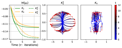
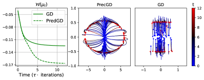
Figure 4: (Left) Value of $\mathcal{W}$ over time and trajectory of particles using $K_{4}$ and $K_{4}^{\Sigma}$ as interaction kernels. (Right) Value of $\mathcal{W}$ over time and trajectory of particles for the Wasserstein gradient descent and preconditioned Wasserstein gradient descent (with the ideal preconditioner $h^{*}(x)=\frac{1}{2}x^{T}\Sigma x$).

Details of Section 5.

We detail in this Section the first experiment of Section 5. We aim at minimizing the interaction energy $\mathcal{W}(\mu)=\iint W(x-y)\ \mathrm{d}\mu(x)\mathrm{d}\mu(y)$ for $W(z)=\frac{1}{4}\|z\|_{2}^{4}-\frac{1}{2}\|z\|_{2}^{2}$. It is well-known that the stationary solution of its gradient flow is a Dirac ring [26]. Since the stationary solution is translation invariant, we project the measures to be centered.

We study here two Bregman potentials which are also interaction energies. First, observing that $\nabla^{2}W(z)=2zz^{T}+\big{(}\|z\|_{2}^{2}-1\big{)}I_{d}$, we have for all $z$,

$$\|\nabla^{2}W\|_{\mathrm{op}}\leq 2\|z\|_{2}^{2}+\|z\|_{2}^{2}+1=3\|z\|_{2}^{2}+1=p_{2}(\|z\|_{2}),$$ (120)

with $p_{2}(t)=3t^{2}+1$. Thus, by [81, Remark 2], $W$ is $\beta$-smooth relative to $K_{4}(z)=\frac{1}{4}\|z\|_{2}^{4}+\frac{1}{2}\|z\|_{2}^{2}$ with $\beta=4$. Thus, using Proposition 21, $\tilde{\mathcal{W}}_{\mu}$ is $\beta$-smooth relative to $\phi_{\mu}(\mathrm{T})=\iint K\big{(}\mathrm{T}(x)-\mathrm{T}(x^{\prime})\big{)}\ \mathrm{d}\mu(x)\mathrm{d}\mu(x^{\prime})$ for all $\mu$, and we can apply Proposition 2.

Under the additional hypothesis that the measures are compactly supported, and thus there exists $M>0$ such that $\|x\|_{2}^{2}\leq M$ for $\mu$-almost every $x$, we can also show that $W$ is $\beta$-smooth relative to $K_{2}(z)=\frac{1}{2}\|z\|_{2}^{2}$. Indeed, on one hand, $\nabla^{2}K=I_{d}$ and $\nabla^{2}W(z)=2zz^{T}+\big{(}\|z\|_{2}^{2}-1\big{)}I_{d}$. Thus, for all $v,z\in\mathbb{R}^{d}$,

$$v^{T}\nabla^{2}W(z)v=2\langle z,v\rangle^{2}+(\|z\|_{2}^{2}-1)\|v\|_{2}^{2}\leq 3\|z\|_{2}^{2}\|v\|_{2}^{2}\leq 3M\|v\|_{2}^{2}=3Mv^{T}\nabla^{2}K(z)v.$$ (121)

In Figure 6, we plot the evolution of $\mathcal{W}$ along the flows obtained with these two Bregman potential, starting from $\mu_{0}=\mathcal{N}(0,0.25^{2}I_{2})$ for $n=100$ particles, with a step size of $\tau=0.1$ for 120 epochs.

Ill-conditioned interaction energy.

We also study the minimization of an interaction energy with an ill-conditioned kernel $W(z)=\frac{1}{4}(z^{T}\Sigma^{-1}z)^{2}-\frac{1}{2}z^{T}\Sigma^{-1}z$ where $\Sigma\in S_{d}^{++}(\mathbb{R})$ but is possibly badly conditioned, i.e. the ratio between the largest and smallest eigenvalues is big. In this case, the stationary solution becomes an ellipsoid instead of a ring. In our experiments, we take $\Sigma=\mathrm{diag}(100,0.1)$. For each scheme, we use $\mu_{0}=\mathcal{N}(0,0.25^{2}I_{2})$, $n=100$ particles and a step size of $\tau=0.1$.

On Figure 2, we use Bregman potentials which take into account this conditioning, namely we use $K_{2}^{\Sigma}(z)=\frac{1}{2}z^{T}\Sigma^{-1}z$ and $K_{4}^{\Sigma}(z)=\frac{1}{4}(z^{T}\Sigma^{-1}z)^{2}-\frac{1}{2}(z^{T}\Sigma^{-1}z)$, and we observe that the convergence is much faster compared to the same kernels without preconditioning. For $K_{2}^{\Sigma}(z)=\frac{1}{2}z^{T}\Sigma^{-1}z$, the scheme becomes

$$(\nabla K\star\mu_{k+1})\circ\mathrm{T}_{k+1}=\nabla K\star\mu_{k}-\gamma\nabla_{\mathrm{W}_{2}}\mathcal{F}(\mu_{k})$$ (122)

$$\iff\Sigma^{-1}\big{(}\mathrm{T}_{k+1}-m(\mu_{k+1})\big{)}=\Sigma^{-1}\big{(}\mathrm{Id}-m(\mu_{k})\big{)}-\gamma\Sigma^{-1}(\mathrm{Id}^{T}\Sigma^{-1}\mathrm{Id}-1)\mathrm{Id}$$

$$\iff\mathrm{T}_{k+1}-m(\mu_{k+1})=\mathrm{Id}-m(\mu_{k})-\gamma(\mathrm{Id}^{T}\Sigma^{-1}\mathrm{Id}-1)\mathrm{Id}.$$

Thus, we see that $\Sigma^{-1}$ has less influence which might explain the faster convergence.

Similarly as in the not preconditioned case, using that $\nabla^{2}W(z)=2\Sigma^{-1}zz^{T}\Sigma^{-1}+(z^{T}\Sigma^{-1}z-1)\Sigma^{-1}$, we can show that

$$v^{T}\nabla^{2}W(z)v=2\langle z,v\rangle_{\Sigma^{-1}}^{2}+(\|z\|_{\Sigma^{-1}}^{2}-1)\|v\|_{\Sigma^{-1}}^{2}\leq 3M\|v\|_{\Sigma^{-1}}^{2}=3Mv^{T}\nabla^{2}K(z)v.$$ (123)

For the sake of comparison, we also report on Figure 4 the trajectories of particles for the use of $K_{4}$ and $K_{4}^{\Sigma}$, as well as of the usual Wasserstein gradient descent and the preconditioned Wasserstein gradient descent obtained with $h^{*}(x)=\frac{1}{2}x^{T}\Sigma x$ (which is equivalent with the Mirror Descent with $\phi_{\mu}^{V}$ as Bregman potential and $V(x)=\frac{1}{2}x^{T}\Sigma^{-1}x$). We observe almost the same trajectories as $K_{2}$, which would indicate that the target is also smooth compared to $\phi_{\mu}^{V}$.

Runtime.

These experiments were run on a personal Laptop with a CPU Intel Core i5-9300H. For the interaction energy as Bregman potential, running the algorithm with Newton’s method for $n=100$ particles in dimension $d=2$ for $120$ epochs took about 5mn for $K_{2}$ and $K_{2}^{\Sigma}$, and about 1h for $K_{4}$ and $K_{4}^{\Sigma}$.

G.3 Mirror descent on Gaussians

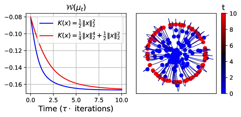
Figure 5: (Left) Value of $\mathcal{W}$ along the flow for two difference interaction Bregman potentials, (Right) Trajectories of particles to minimize $\mathcal{W}$.

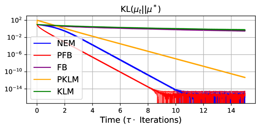
Figure 6: Convergence towards Gaussian $\mathcal{N}(0,D)$ with $D$ diagonal and uniformly sampled on $[0,50]^{10}$.

As the Mirror Descent scheme cannot be computed in closed-form for Bregman potential which are not potential energies, and thus are computationally costly, we propose here to restrain ourselves to the Gaussian setting.

We choose as target distribution $\nu=\mathcal{N}(0,\Sigma)$ for $\Sigma$ a symmetric positive definite matrix in $\mathbb{R}^{10\times 10}$, and thus the functional to be optimized is $\mathcal{F}(\mu)=\int V\mathrm{d}\mu+\mathcal{H}(\mu)$ with $V(x)=\frac{1}{2}x^{T}\Sigma^{-1}x$. The initial distribution is always chosen as $\mu_{0}=\mathcal{N}(0,I_{d})$. In all cases, the step size is chosen as $\tau=0.01$, and we run the scheme for 1500 iterations. For the target distributions, we sample 20 random covariances of the form $\Sigma=UDU^{T}$ with $D$ evenly spaced in log scale between $1$ and $100$, and $U\in\mathbb{R}^{10\times 10}$ chosen as a uniformly random orthogonal matrix, as in [40], and we report the averaged KL divergence over iterations in Figure 2. We add on Figure 6 the same experiments with targets of the form $\mathcal{N}(0,D)$ where $D$ is a diagonal matrix on $\mathbb{R}^{10\times 10}$ sampled uniformly over $[0,50]^{10}$. We compare here the Forward-Backward (FB) scheme of [40], the ideally preconditioned Forward-Backward scheme (PFB), which uses the closed-form (115) derived in Appendix F with $\Lambda=\Sigma$, the Mirror Descent with negative entropy Bregman potential (NEM), whose closed-form was derived in Section D.3

$$\forall k\geq 0,\ \Sigma_{k+1}^{-1}=\big{(}(1-\tau)\Sigma_{k}^{-1}+\tau\Sigma^{-1}\big{)}^{T}\Sigma_{k}\big{(}(1-\tau)\Sigma_{k}^{-1}+\tau\Sigma^{-1}\big{)}.$$ (124)

We also experiment with the KL divergence as Bregman potential (KLM) and the ideally preconditioned KL divergence (PKLM). We observe that, even though the objective is convex relative to the Bregman potential, this scheme does not always converge. It might be due to its gradient which might not always be invertible.color=violet!30,size=] PCA: à rediscuter, parce que c’est aussi possible que ce soit un pbm de schéma du type ss-gradient

Remark 2.

We note that using as Bregman potential $\phi_{\mu}(\mathrm{T})=\int\psi\circ\mathrm{T}\mathrm{d}\mu$ for $\psi(x)=\frac{1}{2}x^{T}\Lambda^{-1}x$ is equivalent with using a preconditioner with $h^{*}(x)=\frac{1}{2}x^{T}\Lambda x$.

Analysis of the convergence.

It is well-known that along the Wasserstein gradient flow of the KL divergence starting from a Gaussian and with a Gaussian target (Ornstein-Uhlenbeck process), the measures stay Gaussian [118]. Thus, the Forward-Backward scheme has Gaussian iterates at each step [101, 40]. We also use a linearly preconditioned Forward-Backward scheme, which closed-form is derived in (115) (Appendix F). For the Bregman potential, we choose $\phi_{\mu}(\mathrm{T})=\int\psi\circ\mathrm{T}\ \mathrm{d}\mu$ for $\psi(x)=\frac{1}{2}x^{T}\Sigma x$. In this situation, $\mathcal{G}(\mu)=\int V\mathrm{d}\mu$ is 1-smooth and 1-convex relative to $\phi_{\mu}$. Thus, we can apply Proposition 23. We refer to Appendix F for more details on the convexity of $\mathcal{H}$.

For Bregman potentials whose gradient is not affine, the distributions do not necessarily stay Gaussian along the flows. Thus, we work on the Bures-Wasserstein space and use the Bures-Wasserstein gradient, i.e. we project the gradient on the space of affine maps with symmetric linear term, i.e. of the form $\mathrm{T}(x)=b+S(x-m)$ with $S\in S_{d}(\mathbb{R})$ [40]. We refer to [68, 40] for more details on this submanifold. This can be seen as performing Variational Inference. We derive the closed-form of the different schemes in Section D.3.

Even though these procedures do not fit exactly the theory developed in this work, we show the relative smoothness of $\mathcal{F}$ relative to $\mathcal{H}$ along the curve $\mu_{t}=\big{(}(1-t)\mathrm{Id}+t\mathrm{T}_{k+1}\big{)}_{\#}\mu_{k}$ under the hypothesis that the covariances matrices have bounded eigenvalues. Moreover, since $\mathrm{d}_{\tilde{\mathcal{F}}_{\mu}}=\mathrm{d}_{\phi_{\mu}^{V}}+\mathrm{d}_{\tilde{\mathcal{H}}_{\mu}}\geq\mathrm{d}_{\tilde{\mathcal{H}}_{\mu}}$, $\mathcal{F}$ is also 1-convex relative to $\mathcal{H}$.

Proposition 25.

Let $\lambda>0$, $\mathcal{F}(\mu)=\int V\mathrm{d}\mu+\mathcal{H}(\mu)$ with $V(x)=\frac{1}{2}x^{T}\Sigma^{-1}x$ where $\Sigma\in S_{d}^{++}(\mathbb{R})$ and $\Sigma\preceq\lambda I_{d}$. Suppose that for all $k\geq 0$, $(1-\tau)\Sigma_{k+1}\Sigma_{k}^{-1}+\tau\Sigma_{k+1}\Sigma^{-1}\succeq 0$. Then, $\mathcal{F}$ is smooth relative to $\mathcal{H}$ along $\mu_{t}=\big{(}(1-t)\mathrm{Id}+t\mathrm{T}_{k+1})_{\#}\mu_{k}$ where $\mu_{k}=\mathcal{N}(0,\Sigma_{k})$ with $\Sigma_{k}\in S_{d}^{++}(\mathbb{R})$, $\Sigma_{k}\preceq\lambda I_{d}$.

Proof.

See Section H.12. ∎

G.4 Single-cell experiments

First, we provide more details on the experiment on single cells of Section 5. Then, we detail a second experiment comparing the method with using a static map.

Details on the metrics.

We show the benefits of using the polynomial preconditioner over the single-cell datasets for different metrics. The first one considered is the Sliced-Wasserstein distance [95, 16], defined as

$$\forall\mu,\nu\in\mathcal{P}_{2}(\mathbb{R}^{d}),\ \mathrm{SW}_{2}^{2}(\mu,\nu)=\int_{S^{d-1}}\mathrm{W}_{2}^{2}(P^{\theta}_{\#}\mu,P^{\theta}_{\#}\nu)\ \mathrm{d}\lambda(\theta),$$ (125)

where $S^{d-1}=\{\theta\in\mathbb{R}^{d},\ \|\theta\|_{2}=1\}$, $\lambda$ denotes the uniform distribution on $S^{d-1}$ and for all $\theta\in S^{d-1}$, $x\in\mathbb{R}^{d}$, $P^{\theta}(x)=\langle x,\theta\rangle$. For $\mathcal{F}(\mu)=\frac{1}{2}\mathrm{SW}_{2}^{2}(\mu,\nu)$, the Wasserstein gradient can be computed as [18]

$$\nabla_{\mathrm{W}_{2}}\mathcal{F}(\mu)=\int_{S^{d-1}}\psi_{\theta}^{\prime}\big{(}P^{\theta}(x)\big{)}\theta\ \mathrm{d}\lambda(\theta),$$ (126)

where, for $t\in\mathbb{R}$, $\psi_{\theta}^{\prime}(t)=t-F_{P^{\theta}_{\#}\nu}^{-1}\big{(}F_{P^{\theta}_{\#}\mu}(t)\big{)}$ with $F_{P^{\theta}_{\#}\mu}$ the cumulative distribution function of $P^{\theta}_{\#}\mu$. In practice, we compute SW and its gradient using a Monte-Carlo approximation by first drawing $L$ uniform random directions $\theta_{1},\dots,\theta_{L}$.

The second one considered is the Sinkhorn divergence [47] defined as

$$\forall\mu,\nu\in\mathcal{P}_{2}(\mathbb{R}^{d}),\ \mathrm{S}_{\varepsilon,2}^{2}(\mu,\nu)=\mathrm{OT}_{\varepsilon}(\mu,\nu)-\frac{1}{2}\mathrm{OT}_{\varepsilon}(\mu,\mu)-\frac{1}{2}\mathrm{OT}_{\varepsilon}(\nu,\nu),$$ (127)

with

$$\mathrm{OT}_{\varepsilon}(\mu,\nu)=\inf_{\gamma\in\Pi(\mu,\nu)}\ \int\|x-y\|_{2}^{2}\ \mathrm{d}\gamma(x,y)+\varepsilon\mathrm{KL}(\gamma||\mu\otimes\nu).$$ (128)

The Wasserstein gradient of $\mathrm{S}_{\varepsilon,2}^{2}$ is simply obtained as the potential [47]. Finally, we also consider the energy distance, defined as

$$\forall\mu,\nu\in\mathcal{P}_{2}(\mathbb{R}^{d}),\ \mathrm{ED}(\mu,\nu)=-\iint\|x-y\|_{2}\ \mathrm{d}(\mu-\nu)(x)\mathrm{d}(\mu-\nu)(y).$$ (129)

To compute its Wasserstein gradient, we use the sliced procedure of [56].

Parameters chosen.

For all the metrics, we fixed the step size at $\tau=1$. To choose the parameter $a$ of the preconditioner $h^{*}(x)=(\|x\|_{2}^{a}+1)^{1/a}-1$, we ran a grid search over $a\in\{1.25,1.5,1.75\}$ for a random treatment, and used it for all the others. In particular, we used for the dataset 4i $a=1.5$ for the Sinkhorn divergence and for SW, and $a=1.75$ for the energy distance. For the scRNAseq dataset, we used $a=1.25$ for the Sinkhorn divergence and SW, and $a=1.5$ for the energy distance. We note that for the dataset 4i, the data lie in dimension $d=48$ and $d=50$ for scRNAseq. For all the metrics, we first sampled 4096 particles from the source (untreated) dataset, and used in average between 2000 and 3000 samples from the target dataset. For the test value, we also added 40% of unseen cells following [20]. Note that we reported the results in Figure 3 for 3 different initializations for each treatment, and reported these results with their mean. We report the results using a fixed relative tolerance $\mathrm{tol}=10^{-3}$, i.e. at the first iteration where $|\mathcal{F}(\mu_{k})-\mathcal{F}(\mu_{k-1})|/\mathcal{F}(\mu_{k-1})\leq\mathrm{tol}$, with a maximum value of iterations of $10^{4}$. For the Sinkhorn divergence, we chose $\varepsilon$ as $10^{-1}$ time the variance of the target. Finally, for SW and the computation of the gradient of the energy distance, we used a Monte-Carlo approximation with $L=1024$ projections.

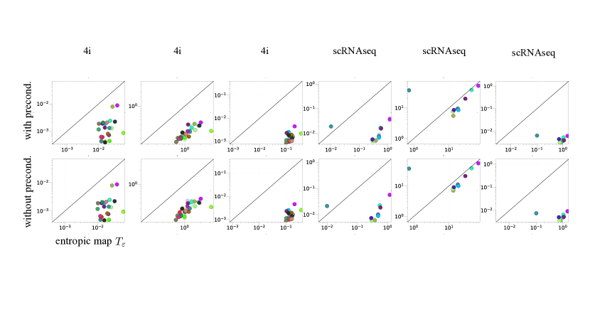
Figure 7: Preconditioned GD and (vanilla) GD vs. the entropic map $T_{\varepsilon}$ [94] to predict the responses of cell populations to cancer treatments on 4i and scRNAseq datasets, providing respectively 34 and 9 treatment responses. For each profiling technology and each treatment, we have a pair $(\mu_{i},\nu_{i})$ of source (untreated) cells and target (treated) cells. For each pair $(\mu_{i},\nu_{i})$, with both preconditioned GD and vanilla GD, we minimize the functional $\mathcal{F}(\mu)=D(\mu,\nu_{i})$–with D a metric–to recover the effect of the perturbation. In both cases, the prediction is obtained by $\hat{\mu_{i}}=\min_{\mu}\mathcal{F}(\mu)$. We then fit an entropic map $T_{\varepsilon}$ and predict $T_{\varepsilon}\sharp\mu_{i}$. We then compare the objective function values $\mathcal{F}(\hat{\mu_{i}})$ and $\mathcal{F}(T_{\varepsilon}\sharp\hat{\mu_{i}})$. A point below the diagonal $y=x$ then refers to an experiment in which (preconditioned) WGD provides a better estimate of the perturbed population.

Comparison to an OT static map.

We now compare the prediction of the response of cells to a perturbation using Wasserstein gradient descent, with and without preconditioning, to the one provided by a static estimator, the entropic map $T_{\varepsilon}$ [94]. This experiment motivates the use of a dynamic procedure, iterating multiple steps to map the unperturbed population $\mu$ to the perturbed population $\nu$, instead of a unique static step. We use the proteomic dataset [20] as the one considered in 3. We use the default OTT-JAX [35] of $T_{\varepsilon}$. The results are shown in Figure 7.

Runtime.

For this experiment, we used a GPU Tesla P100-PCIE-16GB. Depending on the convergence and on the metric considered, each run took in between 30s and 10mn. So in total, it took a few hundred of hours of computation time.

G.5 Mirror descent on the simplex

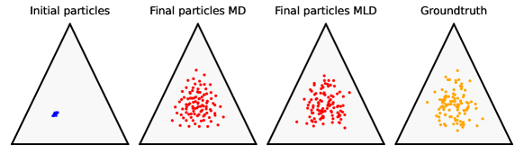
(a)

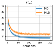
(b)

Figure 8: (Left) Samples from a Dirichlet posterior distribution for Mirror Descent (MD) and Mirror Langevin (MLD). (Right) Evolution of the objective averaged over 20 different initialisations.

We can also leverage the mirror map to perform sampling in constrained spaces. This has received a lot of attention recently either through mirror Langevin methods [3, 30, 108], diffusion methods [75, 48], mirror SVGD [106, 105] or other MCMC algorithms [87, 49].

The goal here is to sample from a Dirichlet distribution, i.e. from a distribution $\nu\propto e^{-V}$ where $V(x)=-\sum_{i=1}^{d}a_{i}\log(x_{i})-a_{d+1}\log\left(1-\sum_{i=1}^{d}x_{i}\right)$. To sample from such a distribution, we minimize the Kullback-Leibler divergence, i.e. $\mathcal{F}(\mu)=\operatorname{KL}(\mu||\nu)=\int V\ \mathrm{d}\mu+\mathcal{H}(\mu)$. To stay on the (open) simplex $\Delta_{d}=\{x\in\mathbb{R}^{d+1},x_{i}>0,\sum_{i=1}^{d+1}x_{i}<1\}$, we use the mirror map $\phi(\mu)=\int\psi\mathrm{d}\mu$ with $\psi(x)=\sum_{i=1}^{d}x_{i}\log(x_{i})+(1-\sum_{i}x_{i})\log(1-\sum_{i}x_{i})$ for which

$$\nabla\psi(x)=\left(\log x_{i}-\log\big(1-\sum_{j}x_{j}\big{missing})\right)_{i},\quad\nabla\psi^{*}(y)=\left(\frac{e^{y_{i}}}{1+\sum_{j}e^{y_{j}}}\right)_{i}.$$ (130)

The scheme here is given by $\mathrm{T}_{k+1}=\nabla\psi^{*}\circ(\nabla\psi-\gamma\nabla_{\mathrm{W}_{2}}\mathcal{F}(\mu_{k}))$, where $\nabla_{\mathrm{W}_{2}}\mathcal{F}(\mu_{k})=\nabla V+\nabla\log\mu_{k}$, with the density of $\mu_{k}$ estimated through a Kernel Density Estimator (KDE). We plot on Figure 8a the results obtained for $d=2$, $a_{1}=a_{2}=a_{3}=6$ and 100 samples. We also report the results for the Mirror Langevin Dynamic (MLD) algorithm, which provide iid samples, which are thus less ordered. We plot the evolution of the $\mathrm{KL}$ over iterations on Figure 8b (where the entropy is estimated using the Kozachenko-Leonenko estimator [39]).

The KDE used here will not scale well with the dimension, however, different methods have been recently propose to overcome this issue, such as using projection on lower dimensional subspaces [116], or using neural networks to learn ratio density estimators [5, 117, 46].

Appendix H Proofs

H.1 Proof of Proposition 1

Let $\mu,\rho\in\mathcal{P}_{2,\mathrm{ac}}(\mathbb{R}^{d})$ and $\nu\in\mathcal{P}_{2}(\mathbb{R}^{d})$. Define $\mathrm{T}_{\phi_{\mu}}^{\mu,\nu}=\operatorname*{argmin}_{\mathrm{T}_{\#}\mu=\nu}\ \mathrm{d}_{\phi_{\mu}}(\mathrm{T},\mathrm{Id})$, $\mathrm{U}_{\phi_{\rho}}^{\rho,\nu}=\operatorname*{argmin}_{\mathrm{U}_{\#}\rho=\nu}\ \mathrm{d}_{\phi_{\rho}}(\mathrm{U},\mathrm{Id})$ and let $\mathrm{S}\in L^{2}(\mu)$ such that $\mathrm{S}_{\#}\mu=\rho$. Then, noticing that $\gamma=(\mathrm{T}_{\phi_{\mu}}^{\mu,\nu},\mathrm{S})_{\#}\mu\in\Pi(\nu,\rho)$, we have

$$\mathrm{d}_{\phi_{\mu}}(\mathrm{T}_{\phi_{\mu}}^{\mu,\nu},\mathrm{S}) =\phi\big{(}(\mathrm{T}_{\phi_{\mu}}^{\mu,\nu})_{\#}\mu\big{)}-\phi(\mathrm{S}_{\#}\nu)-\int\langle\nabla_{\mathrm{W}_{2}}\phi(\mathrm{S}_{\#}\mu)(y),x-y\rangle\ \mathrm{d}(\mathrm{T}_{\phi_{\mu}}^{\mu,\nu},\mathrm{S})_{\#}\mu(x,y)$$ (131)

$$=\phi(\nu)-\phi(\rho)-\int\langle\nabla_{\mathrm{W}_{2}}\phi(\rho)(y),x-y\rangle\ \mathrm{d}\gamma(x,y)$$

$$\geq\mathrm{W}_{\phi}(\nu,\rho)=\mathrm{d}_{\phi_{\rho}}(\mathrm{U}_{\phi_{\rho}}^{\rho,\nu},\mathrm{Id}).$$

In the last line, we used Proposition 13, i.e. that the optimal coupling is of the form $(\mathrm{U}_{\phi_{\rho}}^{\rho,\nu},\mathrm{Id})_{\#}\rho$.

H.2 Proof of Proposition 2

Let $\mathrm{T}_{k+1}=\operatorname*{argmin}_{\mathrm{T}\in L^{2}(\mu_{k})}\ \tau\langle\nabla_{\mathrm{W}_{2}}\mathcal{F}(\mu_{k}),\mathrm{T}-\mathrm{Id}\rangle_{L^{2}(\mu_{k})}+\mathrm{d}_{\phi_{\mu_{k}}}(\mathrm{T},\mathrm{Id})$. Applying the 3-point inequality (Lemma 27) with $\psi(\mathrm{T})=\tau\langle\nabla_{\mathrm{W}_{2}}\mathcal{F}(\mu_{k}),\mathrm{T}-\mathrm{Id}\rangle_{L^{2}(\mu_{k})}$ which is convex, $\mathrm{T}_{0}=\mathrm{Id}$ and $\mathrm{T}^{*}=\mathrm{T}_{k+1}$, we get for all $\mathrm{T}\in L^{2}(\mu_{k})$,

$$\tau\langle\nabla_{\mathrm{W}_{2}}\mathcal{F}(\mu_{k}),\mathrm{T}-\mathrm{Id}\rangle_{L^{2}(\mu_{k})}+\mathrm{d}_{\phi_{\mu_{k}}}(\mathrm{T},\mathrm{Id})$$ (132)

$$\geq\tau\langle\nabla_{\mathrm{W}_{2}}\mathcal{F}(\mu_{k}),\mathrm{T}_{k+1}-\mathrm{Id}\rangle_{L^{2}(\mu_{k})}+\mathrm{d}_{\phi_{\mu_{k}}}(\mathrm{T}_{k+1},\mathrm{Id})+\mathrm{d}_{\phi_{\mu_{k}}}(\mathrm{T},\mathrm{T}_{k+1}),$$

which is equivalent to

$$\langle\nabla_{\mathrm{W}_{2}}\mathcal{F}(\mu_{k}),\mathrm{T}_{k+1}-\mathrm{Id}\rangle_{L^{2}(\mu_{k})}+\frac{1}{\tau}\mathrm{d}_{\phi_{\mu_{k}}}(\mathrm{T}_{k+1},\mathrm{Id})$$ (133)

$$\leq\langle\nabla_{\mathrm{W}_{2}}\mathcal{F}(\mu_{k}),\mathrm{T}-\mathrm{Id}\rangle_{L^{2}(\mu_{k})}+\frac{1}{\tau}\mathrm{d}_{\phi_{\mu_{k}}}(\mathrm{T},\mathrm{Id})-\frac{1}{\tau}\mathrm{d}_{\phi_{\mu_{k}}}(\mathrm{T},\mathrm{T}_{k+1}).$$

By the $\beta$-smoothness of $\tilde{\mathcal{F}}_{\mu_{k}}$ relative to $\phi_{\mu_{k}}$, we also have

$$\mathrm{d}_{\tilde{\mathcal{F}}_{\mu_{k}}}(\mathrm{T}_{k+1},\mathrm{Id})=\tilde{\mathcal{F}}_{\mu_{k}}(\mathrm{T}_{k+1})-\tilde{\mathcal{F}}_{\mu_{k}}(\mathrm{Id})-\langle\nabla_{\mathrm{W}_{2}}\mathcal{F}(\mu_{k}),\mathrm{T}_{k+1}-\mathrm{Id}\rangle_{L^{2}(\mu_{k})}\leq\beta\mathrm{d}_{\phi_{\mu_{k}}}(\mathrm{T}_{k+1},\mathrm{Id})$$ (134)

$$\iff\tilde{\mathcal{F}}_{\mu_{k}}(\mathrm{T}_{k+1})\leq\tilde{\mathcal{F}}_{\mu_{k}}(\mathrm{Id})+\langle\nabla_{\mathrm{W}_{2}}\mathcal{F}(\mu_{k}),\mathrm{T}_{k+1}-\mathrm{Id}\rangle_{L^{2}(\mu_{k})}+\beta\mathrm{d}_{\phi_{\mu_{k}}}(\mathrm{T}_{k+1},\mathrm{Id}).$$

Moreover, since $\beta\leq\frac{1}{\tau}$, this inequality implies (by non-negativity of $\mathrm{d}_{\phi_{\mu_{k}}}$),

$$\tilde{\mathcal{F}}_{\mu_{k}}(\mathrm{T}_{k+1})\leq\tilde{\mathcal{F}}_{\mu_{k}}(\mathrm{Id})+\langle\nabla_{\mathrm{W}_{2}}\mathcal{F}(\mu_{k}),\mathrm{T}_{k+1}-\mathrm{Id}\rangle_{L^{2}(\mu_{k})}+\frac{1}{\tau}\mathrm{d}_{\phi_{\mu_{k}}}(\mathrm{T}_{k+1},\mathrm{Id}).$$ (135)

Then, using the inequality (133), we obtain for all $\mathrm{T}\in L^{2}(\mu_{k})$,

$$\tilde{\mathcal{F}}_{\mu_{k}}(\mathrm{T}_{k+1}) \leq\tilde{\mathcal{F}}_{\mu_{k}}(\mathrm{Id})+\langle\nabla_{\mathrm{W}_{2}}\mathcal{F}(\mu_{k}),\mathrm{T}-\mathrm{Id}\rangle_{L^{2}(\mu_{k})}+\frac{1}{\tau}\mathrm{d}_{\phi_{\mu_{k}}}(\mathrm{T},\mathrm{Id})-\frac{1}{\tau}\mathrm{d}_{\phi_{\mu_{k}}}(\mathrm{T},\mathrm{T}_{k+1})$$ (136)

Observing that $\tilde{\mathcal{F}}_{\mu_{k}}(\mathrm{T}_{k+1})=\mathcal{F}(\mu_{k+1})$ and $\tilde{\mathcal{F}}_{\mu_{k}}(\mathrm{Id})=\mathcal{F}(\mu_{k})$, we get

$$\mathcal{F}(\mu_{k+1})\leq\mathcal{F}(\mu_{k})+\langle\nabla_{\mathrm{W}_{2}}\mathcal{F}(\mu_{k}),\mathrm{T}-\mathrm{Id}\rangle_{L^{2}(\mu_{k})}+\frac{1}{\tau}\mathrm{d}_{\phi_{\mu_{k}}}(\mathrm{T},\mathrm{Id})-\frac{1}{\tau}\mathrm{d}_{\phi_{\mu_{k}}}(\mathrm{T},\mathrm{T}_{k+1}).$$ (137)

Finally, setting $\mathrm{T}=\mathrm{Id}$, we obtain the result:

$$\mathcal{F}(\mu_{k+1})\leq\mathcal{F}(\mu_{k})-\frac{1}{\tau}\mathrm{d}_{\phi_{\mu_{k}}}(\mathrm{Id},\mathrm{T}_{k+1}).$$ (138)

H.3 Proof of Proposition 3

Let $\nu\in\mathcal{P}_{2}(\mathbb{R}^{d})$, and $\mathrm{T}=\operatorname*{argmin}_{\mathrm{T},\mathrm{T}_{\#}\mu_{k}=\nu}\ \mathrm{d}_{\phi_{\mu_{k}}}(\mathrm{T},\mathrm{Id})$. From the relative convexity hypothesis, we have

$$\mathrm{d}_{\tilde{\mathcal{F}}_{\mu_{k}}}(\mathrm{T},\mathrm{Id})\geq\alpha \mathrm{d}_{\phi_{\mu_{k}}}(\mathrm{T},\mathrm{Id})$$ (139)

$$\iff\tilde{\mathcal{F}}_{\mu_{k}}(\mathrm{T})-\tilde{\mathcal{F}}_{\mu_{k}}(\mathrm{Id})-\langle\nabla_{\mathrm{W}_{2}}\mathcal{F}(\mu_{k}),\mathrm{T}-\mathrm{Id}\rangle_{L^{2}(\mu_{k})}\geq\alpha\mathrm{d}_{\phi_{\mu_{k}}}(\mathrm{T},\mathrm{Id})$$

$$\iff\tilde{\mathcal{F}}_{\mu_{k}}(\mathrm{T})-\alpha\mathrm{d}_{\phi_{\mu_{k}}}(\mathrm{T},\mathrm{Id})\geq\tilde{\mathcal{F}}_{\mu_{k}}(\mathrm{Id})+\langle\nabla_{\mathrm{W}_{2}}\mathcal{F}(\mu_{k}),\mathrm{T}-\mathrm{Id}\rangle_{L^{2}(\mu_{k})}$$

$$\iff\mathcal{F}(\nu)-\alpha\mathrm{d}_{\phi_{\mu_{k}}}(\mathrm{T},\mathrm{Id})\geq\mathcal{F}(\mu_{k})+\langle\nabla_{\mathrm{W}_{2}}\mathcal{F}(\mu_{k}),\mathrm{T}-\mathrm{Id}\rangle_{L^{2}(\mu_{k})}.$$

Plugging this into (136), we get

$$\mathcal{F}(\mu_{k+1})\leq\mathcal{F}(\nu)+\frac{1}{\tau}\big{(}\mathrm{d}_{\phi_{\mu_{k}}}(\mathrm{T},\mathrm{Id})-\mathrm{d}_{\phi_{\mu_{k}}}(\mathrm{T},\mathrm{T}_{k+1})\big{)}-\alpha\mathrm{d}_{\phi_{\mu_{k}}}(\mathrm{T},\mathrm{Id}).$$ (140)

Then, by definition of $\mathrm{T}$, note that $\mathrm{d}_{\phi_{\mu_{k}}}(\mathrm{T},\mathrm{Id})=\mathrm{W}_{\phi}(\nu,\mu_{k})$, and by 1, we have $\mathrm{d}_{\phi_{\mu_{k}}}(\mathrm{T},\mathrm{T}_{k+1})\geq\mathrm{W}_{\phi}(\nu,\mu_{k+1})$, since $\mathrm{T}_{\#}\mu_{k}=\nu$ and $(\mathrm{T}_{k+1})_{\#}\mu_{k}=\mu_{k+1}$. Thus,

$$\mathcal{F}(\mu_{k+1})-\mathcal{F}(\nu)\leq\left(\frac{1}{\tau}-\alpha\right)\mathrm{W}_{\phi}(\nu,\mu_{k})-\frac{1}{\tau}\mathrm{W}_{\phi}(\nu,\mu_{k+1}).$$ (141)

Observing that $\mathcal{F}(\mu_{k})\leq\mathcal{F}(\mu_{\ell})$ for all $\ell\leq k$ (by Proposition 2 and non-negativity of $\mathrm{d}_{\phi}$ for $\phi$ convex) and that $\mathrm{W}_{\phi}(\nu,\mu)\geq 0$, we can apply Lemma 28 with $f=\mathcal{F}$, $c=\mathcal{F}(\nu)$ and $g=\mathrm{W}_{\phi}(\nu,\cdot)$, and we obtain

$$\forall k\geq 1,\ \mathcal{F}(\mu_{k})-\mathcal{F}(\nu)\leq\frac{\alpha}{\left(\frac{\frac{1}{\tau}}{\frac{1}{\tau}-\alpha}\right)^{k}-1}\mathrm{W}_{\phi}(\nu,\mu_{0})\leq\frac{\frac{1}{\tau}-\alpha}{k}\mathrm{W}_{\phi}(\nu,\mu_{0}).$$ (142)

For the second result, from (141), we get for $\nu=\mu^{*}$ the minimizer of $\mathcal{F}$, since $\mathcal{F}(\mu_{k+1})-\mathcal{F}(\mu^{*})\geq 0$,

$$\mathrm{W}_{\phi}(\mu^{*},\mu_{k+1})\leq\left(1-\alpha\tau\right)\mathrm{W}_{\phi}(\mu^{*},\mu_{k})\leq\left(1-\alpha\tau\right)^{k+1}\mathrm{W}_{\phi}(\mu^{*},\mu_{0}).$$ (143)

H.4 Proof of Proposition 4

Let $k\geq 0$, by the definition of $\mathrm{d}_{\phi_{\mu_{k}}^{h^{*}}}$ and the hypothesis $\mathrm{d}_{\phi_{\mu_{k}}^{h^{*}}}\big{(}\nabla_{\mathrm{W}_{2}}\mathcal{F}(\mu_{k+1})\circ\mathrm{T}_{k+1},\nabla_{\mathrm{W}_{2}}\mathcal{F}(\mu_{k})\big{)}\leq\beta\mathrm{d}_{\tilde{\mathcal{F}}_{\mu_{k}}}(\mathrm{Id},\mathrm{T}_{k+1})$ , we have

$$\phi_{\mu_{k+1}}^{h^{*}}\big{(}\nabla_{\mathrm{W}_{2}}\mathcal{F}(\mu_{k+1})\big{)} =\phi_{\mu_{k}}^{h^{*}}\big{(}\nabla_{\mathrm{W}_{2}}\mathcal{F}(\mu_{k})\big{)}$$ (144)

$$\quad+\langle\nabla{h^{*}}\circ\nabla_{\mathrm{W}_{2}}\mathcal{F}(\mu_{k}),\nabla_{\mathrm{W}_{2}}\mathcal{F}(\mu_{k+1})\circ\mathrm{T}_{k+1}-\nabla_{\mathrm{W}_{2}}\mathcal{F}(\mu_{k})\rangle_{L^{2}(\mu_{k})}$$

$$\quad+\mathrm{d}_{\phi_{\mu_{k}}^{h^{*}}}\big{(}\nabla_{\mathrm{W}_{2}}\mathcal{F}((\mathrm{T}_{k+1})_{\#}\mu_{k})\circ\mathrm{T}_{k+1},\nabla_{\mathrm{W}_{2}}\mathcal{F}(\mu_{k})\big{)}$$

$$\leq\phi_{\mu_{k}}^{h^{*}}\big{(}\nabla_{\mathrm{W}_{2}}\mathcal{F}(\mu_{k})\big{)}$$

$$\quad+\langle\nabla{h^{*}}\circ\nabla_{\mathrm{W}_{2}}\mathcal{F}(\mu_{k}),\nabla_{\mathrm{W}_{2}}\mathcal{F}(\mu_{k+1})\circ\mathrm{T}_{k+1}-\nabla_{\mathrm{W}_{2}}\mathcal{F}(\mu_{k})\rangle_{L^{2}(\mu_{k})}$$

$$\quad+\beta\mathrm{d}_{\tilde{\mathcal{F}}_{\mu_{k}}}(\mathrm{Id},\mathrm{T}_{k+1})$$

$$\leq\phi_{\mu_{k}}^{h^{*}}\big{(}\nabla_{\mathrm{W}_{2}}\mathcal{F}(\mu_{k})\big{)}$$

$$\quad+\langle\nabla{h^{*}}\circ\nabla_{\mathrm{W}_{2}}\mathcal{F}(\mu_{k}),\nabla_{\mathrm{W}_{2}}\mathcal{F}(\mu_{k+1})\circ\mathrm{T}_{k+1}-\nabla_{\mathrm{W}_{2}}\mathcal{F}(\mu_{k})\rangle_{L^{2}(\mu_{k})}$$

$$\quad+\frac{1}{\tau}\mathrm{d}_{\tilde{\mathcal{F}}_{\mu_{k}}}(\mathrm{Id},\mathrm{T}_{k+1}),$$

where we used in the last line that $\tau\leq\frac{1}{\beta}$ and the non-negativity of the Bregman divergence since $\mathcal{F}$ is convex along $t\mapsto\big{(}(1-t)\mathrm{T}_{k+1}+t\mathrm{Id}\big{)}_{\#}\mu_{k}$ and thus by Proposition 11, $\mathrm{d}_{\tilde{\mathcal{F}}_{\mu_{k}}}(\mathrm{Id},\mathrm{T}_{k+1})\geq 0$.

Let $\mathrm{T}\in L^{2}(\mu_{k})$. Then, using the three-point identity (Lemma 26) (with $\mathrm{S}=\mathrm{Id}$, $\mathrm{U}=\mathrm{T}$ and $\mathrm{T}=\mathrm{T}_{k+1}$), and remembering that $\mathrm{T}_{k+1}=\mathrm{Id}-\tau\nabla{h^{*}}\circ\nabla_{\mathrm{W}_{2}}\mathcal{F}(\mu_{k})$, we get

$$\mathrm{d}_{\tilde{\mathcal{F}}_{\mu_{k}}}(\mathrm{Id},\mathrm{T}_{k+1}) =\mathrm{d}_{\tilde{\mathcal{F}}_{\mu_{k}}}(\mathrm{Id},\mathrm{T})-\mathrm{d}_{\tilde{\mathcal{F}}_{\mu_{k}}}(\mathrm{T}_{k+1},\mathrm{T})$$ (145)

$$\quad-\langle\nabla_{\mathrm{W}_{2}}\mathcal{F}\big{(}(\mathrm{T}_{k+1})_{\#}\mu_{k}\big{)}\circ\mathrm{T}_{k+1},\mathrm{Id}-\mathrm{T}_{k+1}\rangle_{L^{2}(\mu_{k})}$$

$$\quad+\langle\nabla_{\mathrm{W}_{2}}\mathcal{F}(\mathrm{T}_{\#}\mu_{k})\circ\mathrm{T},\mathrm{Id}-\mathrm{T}_{k+1}\rangle_{L^{2}(\mu_{k})}$$

$$=\mathrm{d}_{\tilde{\mathcal{F}}_{\mu_{k}}}(\mathrm{Id},\mathrm{T})-\mathrm{d}_{\tilde{\mathcal{F}}_{\mu_{k}}}(\mathrm{T}_{k+1},\mathrm{T})$$

$$\quad+\langle\nabla_{\mathrm{W}_{2}}\mathcal{F}(\mathrm{T}_{\#}\mu_{k})\circ\mathrm{T}-\nabla_{\mathrm{W}_{2}}\mathcal{F}(\mu_{k+1})\circ\mathrm{T}_{k+1},\mathrm{Id}-\mathrm{T}_{k+1}\rangle_{L^{2}(\mu_{k})}$$

$$=\mathrm{d}_{\tilde{\mathcal{F}}_{\mu_{k}}}(\mathrm{Id},\mathrm{T})-\mathrm{d}_{\tilde{\mathcal{F}}_{\mu_{k}}}(\mathrm{T}_{k+1},\mathrm{T})$$

$$\quad+\tau\langle\nabla_{\mathrm{W}_{2}}\mathcal{F}(\mathrm{T}_{\#}\mu_{k})\circ\mathrm{T}-\nabla_{\mathrm{W}_{2}}\mathcal{F}(\mu_{k+1})\circ\mathrm{T}_{k+1},\nabla{h^{*}}\circ\nabla_{\mathrm{W}_{2}}\mathcal{F}(\mu_{k})\rangle_{L^{2}(\mu_{k})}.$$

This is equivalent with

$$\langle\nabla{h^{*}}\circ \nabla_{\mathrm{W}_{2}}\mathcal{F}(\mu_{k}),\nabla_{\mathrm{W}_{2}}\mathcal{F}(\mu_{k+1})\circ\mathrm{T}_{k+1}-\nabla_{\mathrm{W}_{2}}\mathcal{F}(\mu_{k})\rangle_{L^{2}(\mu_{k})}+\frac{1}{\tau}\mathrm{d}_{\tilde{\mathcal{F}}_{\mu_{k}}}(\mathrm{Id},\mathrm{T}_{k+1})$$

$$=\frac{1}{\tau}\mathrm{d}_{\tilde{\mathcal{F}}_{\mu_{k}}}(\mathrm{Id},\mathrm{T})-\frac{1}{\tau}\mathrm{d}_{\tilde{\mathcal{F}}_{\mu_{k}}}(\mathrm{T}_{k+1},\mathrm{T})$$

$$\quad+\langle\nabla_{\mathrm{W}_{2}}\mathcal{F}(\mathrm{T}_{\#}\mu_{k})\circ\mathrm{T}-\nabla_{\mathrm{W}_{2}}\mathcal{F}(\mu_{k}),\nabla{h^{*}}\circ\nabla_{\mathrm{W}_{2}}\mathcal{F}(\mu_{k})\rangle_{L^{2}(\mu_{k})}.$$ (146)

Then, using the definition of $\mathrm{d}_{\phi_{\mu_{k}}^{h^{*}}}\big{(}\nabla_{\mathrm{W}_{2}}\mathcal{F}(\mathrm{T}_{\#}\mu_{k})\circ\mathrm{T},\nabla_{\mathrm{W}_{2}}\mathcal{F}(\mu_{k})\big{)}$, we obtain

$$\langle\nabla{h^{*}}\circ\nabla_{\mathrm{W}_{2}}\mathcal{F}(\mu_{k}),\nabla_{\mathrm{W}_{2}}\mathcal{F}(\mu_{k+1})\circ\mathrm{T}_{k+1}-\nabla_{\mathrm{W}_{2}}\mathcal{F}(\mu_{k})\rangle_{L^{2}(\mu_{k})}+\frac{1}{\tau}\mathrm{d}_{\tilde{\mathcal{F}}_{\mu_{k}}}(\mathrm{Id},\mathrm{T}_{k+1})$$ (147)

$$=\frac{1}{\tau}\mathrm{d}_{\tilde{\mathcal{F}}_{\mu_{k}}}(\mathrm{Id},\mathrm{T})-\frac{1}{\tau}\mathrm{d}_{\tilde{\mathcal{F}}_{\mu_{k}}}(\mathrm{T}_{k+1},\mathrm{T})$$

$$\quad-\mathrm{d}_{\phi_{\mu_{k}}^{h^{*}}}\big{(}\nabla_{\mathrm{W}_{2}}\mathcal{F}(\mathrm{T}_{\#}\mu_{k})\circ\mathrm{T},\nabla_{\mathrm{W}_{2}}\mathcal{F}(\mu_{k})\big{)}+\phi_{\mu_{k}}^{{h^{*}}}\big{(}\nabla_{\mathrm{W}_{2}}\mathcal{F}(\mathrm{T}_{\#}\mu_{k})\circ\mathrm{T}\big{)}-\phi_{\mu_{k}}^{h^{*}}\big{(}\nabla_{\mathrm{W}_{2}}\mathcal{F}(\mu_{k})\big{)}.$$

Plugging this into (144), we get

$$\phi_{\mu_{k+1}}^{h^{*}}\big{(}\nabla_{\mathrm{W}_{2}}\mathcal{F}(\mu_{k+1})\big{)}\leq\phi_{\mu_{k}}^{h^{*}}\big{(}\nabla_{\mathrm{W}_{2}}\mathcal{F}(\mathrm{T}_{\#}\mu_{k})\circ\mathrm{T}\big{)}+\frac{1}{\tau}\mathrm{d}_{\tilde{\mathcal{F}}_{\mu_{k}}}(\mathrm{Id},\mathrm{T})-\frac{1}{\tau}\mathrm{d}_{\tilde{\mathcal{F}}_{\mu_{k}}}(\mathrm{T}_{k+1},\mathrm{T})\\ -\mathrm{d}_{\phi_{\mu_{k}}^{h^{*}}}\big{(}\nabla_{\mathrm{W}_{2}}\mathcal{F}(\mathrm{T}_{\#}\mu_{k})\circ\mathrm{T},\nabla_{\mathrm{W}_{2}}\mathcal{F}(\mu_{k})\big{)}.$$ (148)

For $\mathrm{T}=\mathrm{Id}$, we get

$$\phi_{\mu_{k+1}}^{h^{*}}\big{(}\nabla_{\mathrm{W}_{2}}\mathcal{F}(\mu_{k+1})\big{)}\leq\phi_{\mu_{k}}^{h^{*}}\big{(}\nabla_{\mathrm{W}_{2}}\mathcal{F}(\mu_{k})\big{)}-\frac{1}{\tau}\mathrm{d}_{\tilde{\mathcal{F}}_{\mu_{k}}}(\mathrm{T}_{k+1},\mathrm{Id}).$$ (149)

H.5 Proof of Proposition 5

Let $\mu^{*}\in\mathcal{P}_{2}(\mathbb{R}^{d})$ be the minimizer of $\mathcal{F}$, $k\geq 0$ and $\mathrm{T}=\operatorname*{argmin}_{\mathrm{T}\in L^{2}(\mu_{k}),\mathrm{T}_{\#}\mu_{k}=\mu^{*}}\ \mathrm{d}_{\tilde{\mathcal{F}}_{\mu_{k}}}(\mathrm{Id},\mathrm{T})$. First, observe that since $\mu^{*}$ is the minimizer of $\mathcal{F}$, then $\nabla_{\mathrm{W}_{2}}\mathcal{F}(\mu^{*})=0$ (see e.g. [69, Theorem 3.1]), and thus $\phi_{\mu_{k}}^{h^{*}}(0)={h^{*}}(0)$. Moreover, it induces that $\mathrm{d}_{\tilde{\mathcal{F}}_{\mu_{k}}}(\mathrm{Id},\mathrm{T})=\mathcal{F}(\mu_{k})-\mathcal{F}(\mu^{*})$ and $\mathrm{d}_{\tilde{\mathcal{F}}_{\mu_{k}}}(\mathrm{T}_{k+1},\mathrm{T})=\mathcal{F}(\mu_{k+1})-\mathcal{F}(\mu^{*})$.

Therefore, using (148) and the hypothesis $\alpha\mathrm{d}_{\tilde{\mathcal{F}}_{\mu_{k}}}(\mathrm{Id},\mathrm{T})\leq\mathrm{d}_{\phi_{\mu_{k}}^{h^{*}}}\big{(}0,\nabla_{\mathrm{W}_{2}}\mathcal{F}(\mu_{k})\big{)}$, we get

$$\phi_{\mu_{k+1}}^{h^{*}}\big{(}\nabla_{\mathrm{W}_{2}}\mathcal{F}(\mu_{k+1})\big{)}-{h^{*}}(0) \leq\frac{1}{\tau}\mathrm{d}_{\tilde{\mathcal{F}}_{\mu_{k}}}(\mathrm{Id},\mathrm{T})-\frac{1}{\tau}\mathrm{d}_{\tilde{\mathcal{F}}_{\mu_{k}}}(\mathrm{T}_{k+1},\mathrm{T})-\mathrm{d}_{\phi_{\mu_{k}}^{h^{*}}}\big{(}0,\nabla_{\mathrm{W}_{2}}\mathcal{F}(\mu_{k})\big{)}$$ (150)

$$\leq\frac{1}{\tau}\mathrm{d}_{\tilde{\mathcal{F}}_{\mu_{k}}}(\mathrm{Id},\mathrm{T})-\frac{1}{\tau}\mathrm{d}_{\tilde{\mathcal{F}}_{\mu_{k}}}(\mathrm{T}_{k+1},\mathrm{T})-\alpha\mathrm{d}_{\tilde{\mathcal{F}}_{\mu_{k}}}(\mathrm{Id},\mathrm{T})$$

$$=\left(\frac{1}{\tau}-\alpha\right)\mathrm{d}_{\tilde{\mathcal{F}}_{\mu_{k}}}(\mathrm{Id},\mathrm{T})-\frac{1}{\tau}\mathrm{d}_{\tilde{\mathcal{F}}_{\mu_{k}}}(\mathrm{T}_{k+1},\mathrm{T})$$

$$=\left(\frac{1}{\tau}-\alpha\right)\big{(}\mathcal{F}(\mu_{k})-\mathcal{F}(\mu^{*})\big{)}-\frac{1}{\tau}\big{(}\mathcal{F}(\mu_{k+1})-\mathcal{F}(\mu^{*})\big{)}.$$

Then, applying Lemma 28 with $f=\phi_{\cdot}^{h^{*}}\circ\nabla_{\mathrm{W}_{2}}\mathcal{F}$ (which satisfies $\phi_{\mu_{k+1}}^{h^{*}}\big{(}\nabla_{\mathrm{W}_{2}}\mathcal{F}(\mu_{k+1})\big{)}\leq\phi_{\mu_{k}}^{h^{*}}\big{(}\nabla_{\mathrm{W}_{2}}\mathcal{F}(\mu_{k})\big{)}$ by Proposition 4), $c=h^{*}(0)$ and $g=\mathcal{F}(\cdot)-\mathcal{F}(\mu^{*})\geq 0$, we get

$$\phi_{\mu_{k}}^{h^{*}}\big{(}\nabla_{\mathrm{W}_{2}}\mathcal{F}(\mu_{k})\big{)}-{h^{*}}(0)\leq\frac{\alpha}{\left(\frac{\frac{1}{\tau}}{\frac{1}{\tau}-\alpha}\right)^{k}-1}\big{(}\mathcal{F}(\mu_{0})-\mathcal{F}(\mu^{*})\big{)}\leq\frac{\frac{1}{\tau}-\alpha}{k}\big{(}\mathcal{F}(\mu_{0})-\mathcal{F}(\mu^{*})\big{)}.$$ (151)

Concerning the convergence of $\mathcal{F}(\mu_{k})$, if $\alpha>0$ and ${h^{*}}$ attains its minimum in $0$, then necessarily $\phi_{\mu}^{h^{*}}(\mathrm{T})\geq{h^{*}}(0)$ for all $\mu\in\mathcal{P}_{2}(\mathbb{R}^{d})$ and $\mathrm{T}\in L^{2}(\mu)$. Thus, using (148), we get

$$0\leq\phi_{\mu_{k+1}}^{h^{*}}\big{(}\nabla_{\mathrm{W}_{2}}\mathcal{F}(\mu_{k+1})\big{)}-{h^{*}}(0) \leq\frac{1}{\tau}\mathrm{d}_{\tilde{\mathcal{F}}_{\mu_{k}}}(\mathrm{Id},\mathrm{T})-\frac{1}{\tau}\mathrm{d}_{\tilde{\mathcal{F}}_{\mu_{k}}}(\mathrm{T}_{k+1},\mathrm{T})-\mathrm{d}_{\phi_{\mu_{k}}^{h^{*}}}\big{(}0,\nabla_{\mathrm{W}_{2}}\mathcal{F}(\mu_{k})\big{)}$$

$$\leq\frac{1}{\tau}\big{(}\mathcal{F}(\mu_{k})-\mathcal{F}(\mu^{*})\big{)}-\frac{1}{\tau}\big{(}\mathcal{F}(\mu_{k+1})-\mathcal{F}(\mu^{*})\big{)}$$

$$\quad-\alpha\mathrm{d}_{\tilde{\mathcal{F}}_{\mu_{k}}}(\mathrm{Id},\mathrm{T})$$

$$=\left(\frac{1}{\tau}-\alpha\right)\big{(}\mathcal{F}(\mu_{k})-\mathcal{F}(\mu^{*})\big{)}-\frac{1}{\tau}\big{(}\mathcal{F}(\mu_{k+1})-\mathcal{F}(\mu^{*})\big{)}.$$ (152)

Thus, for all $k\geq 0$,

$$\mathcal{F}(\mu_{k+1})-\mathcal{F}(\mu^{*}) =\left(1-\tau\alpha\right)\big{(}\mathcal{F}(\mu_{k})-\mathcal{F}(\mu^{*})\big{)}$$ (153)

$$\leq\left(1-\tau\alpha\right)^{k+1}\big{(}\mathcal{F}(\mu_{0})-\mathcal{F}(\mu^{*})\big{)}.$$

H.6 Proof of Lemma 9

Let us define $\tilde{\mathcal{G}}_{\mu}:L^{2}(\mu)\times\mathbb{R}^{d}\to\mathbb{R}^{d}$ as for all $\mathrm{T}\in L^{2}(\mu)$, $x\in\mathbb{R}^{d}$,

$$\tilde{\mathcal{G}}_{\mu}(\mathrm{T},x)=\nabla_{\mathrm{W}_{2}}\mathcal{F}(\mathrm{T}_{\#}\mu)(x)=\begin{pmatrix}\frac{\partial}{\partial x_{1}}\frac{\delta\mathcal{F}}{\delta\mu}(\mathrm{T}_{\#}\mu)(x)\\ \vdots\\ \frac{\partial}{\partial x_{d}}\frac{\delta\mathcal{F}}{\delta\mu}(\mathrm{T}_{\#}\mu)(x)\end{pmatrix}=\begin{pmatrix}\tilde{G}_{\mu}^{1}(\mathrm{T},x)\\ \vdots\\ \tilde{G}_{\mu}^{d}(\mathrm{T},x)\end{pmatrix},$$ (154)

with for all $i$, $\tilde{G}_{\mu}^{i}:L^{2}(\mu)\times\mathbb{R}^{d}\to\mathbb{R}$, $\tilde{G}_{\mu}^{i}(\mathrm{T},x)=\frac{\partial}{\partial x_{i}}\frac{\delta\mathcal{F}}{\delta\mu}(\mathrm{T}_{\#}\mu)(x)$. Using the chain rule, for all $x\in\mathbb{R}^{d}$,

$$\frac{\mathrm{d}\tilde{G}_{\mu}^{i}}{\mathrm{d}s}\big{(}\mathrm{T}_{s},\mathrm{T}_{s}(x)\big{)} =\left\langle\nabla_{1}\tilde{G}_{\mu}^{i}\big{(}\mathrm{T}_{s},\mathrm{T}_{s}(x)\big{)},\frac{\mathrm{d}\mathrm{T}_{s}}{\mathrm{d}s}\right\rangle_{L^{2}(\mu)}+\left\langle\nabla_{2}\tilde{G}_{\mu}^{i}\big{(}\mathrm{T}_{s},\mathrm{T}_{s}(x)\big{)},\frac{\mathrm{d}\mathrm{T}_{s}}{\mathrm{d}s}(x)\right\rangle.$$ (155)

On one hand, we have $\nabla_{2}\tilde{G}_{\mu}^{i}\big{(}\mathrm{T}_{s},\mathrm{T}_{s}(x)\big{)}=\nabla\frac{\partial}{\partial x_{i}}\frac{\delta\mathcal{F}}{\delta\mu}\big{(}(\mathrm{T}_{s})_{\#}\mu\big{)}\big{(}\mathrm{T}_{s}(x)\big{)}$. On the other hand, let us compute $\nabla_{1}\tilde{G}_{\mu}^{i}(\mathrm{T},x)$. First, we define the shorthands $\tilde{g}_{\mu}^{x,i}(\mathrm{T})=\tilde{G}_{\mu}^{i}(\mathrm{T},x)=\frac{\partial}{\partial x_{i}}\frac{\delta\mathcal{F}}{\delta\mu}(\mathrm{T}_{\#}\mu)(x)$ and $g^{x,i}(\nu)=\frac{\partial}{\partial x_{i}}\frac{\delta\mathcal{F}}{\delta\mu}(\nu)(x)$. Since $\tilde{g}_{\mu}^{x,i}(\mathrm{T})=g^{x,i}(\mathrm{T}_{\#}\mu)$, applying Proposition 8, we know that $\nabla_{1}\tilde{G}_{\mu}(\mathrm{T},x)=\nabla\tilde{g}_{\mu}^{x,i}(\mathrm{T})=\nabla_{\mathrm{W}_{2}}g^{x,i}(\mathrm{T}_{\#}\mu)\circ T$.

Now, let us compute $\nabla_{\mathrm{W}_{2}}g^{x,i}(\nu)=\nabla\frac{\delta g^{x,i}}{\delta\mu}(\nu)$. Let $\chi$ be such that $\int\mathrm{d}\chi=0$, then using the hypothesis that $\frac{\delta}{\delta\mu}\nabla\frac{\delta\mathcal{F}}{\delta\mu}=\nabla\frac{\delta^{2}\mathcal{F}}{\delta\mu^{2}}$ and the definition of $g^{x,i}$,

$$\int\frac{\delta g^{x,i}}{\delta\mu}(\nu)\ \mathrm{d}\chi =\int\frac{\partial}{\partial x_{i}}\frac{\delta^{2}\mathcal{F}}{\delta\mu^{2}}(\nu)(x,y)\ \mathrm{d}\chi(y).$$ (156)

Thus, $\nabla_{\mathrm{W}_{2}}g^{x,i}(\nu)=\nabla_{y}\frac{\partial}{\partial x_{i}}\frac{\delta^{2}\mathcal{F}}{\delta\mu^{2}}(\nu)(x,y)$.

Putting everything together, we obtain

$$\frac{\mathrm{d}\tilde{G}_{\mu}^{i}}{\mathrm{d}s}\big{(}\mathrm{T}_{s},\mathrm{T}_{s}(x)\big{)} =\left\langle\nabla_{y}\frac{\partial}{\partial x_{i}}\frac{\delta^{2}\mathcal{F}}{\delta\mu^{2}}\big{(}(\mathrm{T}_{s})_{\#}\mu\big{)}\big{(}\mathrm{T}_{s}(x),\mathrm{T}_{s}(\cdot)\big{)},\frac{\mathrm{d}\mathrm{T}_{s}}{\mathrm{d}s}\right\rangle_{L^{2}(\mu)}$$ (157)

$$\quad+\left\langle\nabla\frac{\partial}{\partial x_{i}}\frac{\delta\mathcal{F}}{\delta\mu}\big{(}(\mathrm{T}_{s})_{\#}\mu\big{)}\big{(}\mathrm{T}_{s}(x)\big{)},\frac{\mathrm{d}\mathrm{T}_{s}}{\mathrm{d}s}(x)\right\rangle$$

$$=\int\left\langle\nabla_{y}\frac{\partial}{\partial x_{i}}\frac{\delta^{2}\mathcal{F}}{\delta\mu^{2}}\big{(}(\mathrm{T}_{s})_{\#}\mu\big{)}\big{(}\mathrm{T}_{s}(x),\mathrm{T}_{s}(y)\big{)},\frac{\mathrm{d}\mathrm{T}_{s}}{\mathrm{d}s}(y)\right\rangle\ \mathrm{d}\mu(y)$$

$$\quad+\left\langle\nabla\frac{\partial}{\partial x_{i}}\frac{\delta\mathcal{F}}{\delta\mu}\big{(}(\mathrm{T}_{s})_{\#}\mu\big{)}\big{(}\mathrm{T}_{s}(x)\big{)},\frac{\mathrm{d}\mathrm{T}_{s}}{\mathrm{d}s}(x)\right\rangle,$$

and thus

$$\frac{\mathrm{d}}{\mathrm{d}s}\tilde{\mathcal{G}}_{\mu}\big{(}\mathrm{T}_{s},\mathrm{T}_{s}(x)\big{)}=\int\nabla_{y}\nabla_{x}\frac{\delta^{2}\mathcal{F}}{\delta\mu^{2}}\big{(}(\mathrm{T}_{s})_{\#}\mu\big{)}\big{(}\mathrm{T}_{s}(x),\mathrm{T}_{s}(y)\big{)}\frac{\mathrm{d}\mathrm{T}_{s}}{\mathrm{d}s}(y)\ \mathrm{d}\mu(y)\\ +\nabla^{2}\frac{\delta\mathcal{F}}{\delta\mu}\big{(}(\mathrm{T}_{s})_{\#}\mu\big{)}\big{(}\mathrm{T}_{s}(x)\big{)}\frac{\mathrm{d}\mathrm{T}_{s}}{\mathrm{d}s}(x).$$ (158)

H.7 Proof of Proposition 10

First, recall that by using the chain rule and Proposition 8, $\frac{\mathrm{d}}{\mathrm{d}t}\mathcal{F}(\mu_{t})=\langle\nabla_{\mathrm{W}_{2}}\mathcal{F}(\mu_{t})\circ\mathrm{T}_{t},\frac{\mathrm{d}\mathrm{T}_{t}}{\mathrm{d}t}\rangle_{L^{2}(\mu)}$. Thus, since $\frac{\mathrm{d}^{2}\mathrm{T}_{t}}{\mathrm{d}t^{2}}=0$,

$$\frac{\mathrm{d}^{2}}{\mathrm{d}t^{2}}\mathcal{F}(\mu_{t}) =\frac{\mathrm{d}}{\mathrm{d}t}\left\langle\nabla_{\mathrm{W}_{2}}\mathcal{F}(\mu_{t})\circ\mathrm{T}_{t},\frac{\mathrm{d}\mathrm{T}_{t}}{\mathrm{d}t}\right\rangle_{L^{2}(\mu)}$$ (159)

$$=\left\langle\frac{\mathrm{d}}{\mathrm{d}t}\left(\nabla_{\mathrm{W}_{2}}\mathcal{F}(\mu_{t})\circ\mathrm{T}_{t}\right),\frac{\mathrm{d}\mathrm{T}_{t}}{\mathrm{d}t}\right\rangle_{L^{2}(\mu)}.$$

By Lemma 9,

$$\frac{\mathrm{d}^{2}}{\mathrm{d}t^{2}}\mathcal{F}(\mu_{t}) =\iint\left\langle\nabla_{y}\nabla_{x}\frac{\delta^{2}\mathcal{F}}{\delta\mu^{2}}\big{(}(\mathrm{T}_{t})_{\#}\mu\big{)}\big{(}\mathrm{T}_{t}(x),\mathrm{T}_{t}(y)\big{)}\frac{\mathrm{d}\mathrm{T}_{t}}{\mathrm{d}t}(y),\frac{\mathrm{d}\mathrm{T}_{t}}{\mathrm{d}t}(x)\right\rangle\ \mathrm{d}\mu(y)\mathrm{d}\mu(x)$$ (160)

$$\quad+\int\left\langle\nabla^{2}\frac{\delta\mathcal{F}}{\delta\mu}\big{(}(\mathrm{T}_{t})_{\#}\mu\big{)}\big{(}\mathrm{T}_{t}(x)\big{)}\frac{\mathrm{d}\mathrm{T}_{t}}{\mathrm{d}t}(x),\frac{\mathrm{d}\mathrm{T}_{t}}{\mathrm{d}t}(x)\right\rangle\ \mathrm{d}\mu(x)$$

$$=\iint\left\langle\nabla_{y}\nabla_{x}\frac{\delta^{2}\mathcal{F}}{\delta\mu^{2}}\big{(}(\mathrm{T}_{t})_{\#}\mu\big{)}\big{(}\mathrm{T}_{t}(x),\mathrm{T}_{t}(y)\big{)}v(y),v(x)\right\rangle\ \mathrm{d}\mu(y)\mathrm{d}\mu(x)$$

$$\quad+\int\left\langle\nabla^{2}\frac{\delta\mathcal{F}}{\delta\mu}\big{(}(\mathrm{T}_{t})_{\#}\mu\big{)}\big{(}\mathrm{T}_{t}(x)\big{)}v(x),v(x)\right\rangle\ \mathrm{d}\mu(x)$$

$$=\int\Big{\langle}\int\nabla_{y}\nabla_{x}\frac{\delta^{2}\mathcal{F}}{\delta\mu^{2}}\big{(}(\mathrm{T}_{t})_{\#}\mu\big{)}\big{(}\mathrm{T}_{t}(x),\mathrm{T}_{t}(y)\big{)}v(y)\ \mathrm{d}\mu(y)$$

$$\quad+\nabla^{2}\frac{\delta\mathcal{F}}{\delta\mu}\big{(}(\mathrm{T}_{t})_{\#}\mu\big{)}\big{(}\mathrm{T}_{t}(x)\big{)}v(x),v(x)\Big{\rangle}\ \mathrm{d}\mu(x).$$

H.8 Proof of Proposition 11

1. (c1) $\implies$ (c2). Let $t>0$, $t_{1},t_{2}\in[0,1]$,

   $$\mathcal{F}(\tilde{\mu}_{t}^{t_{1}\to t_{2}})\leq(1-t)\mathcal{F}\big{(}(\mathrm{T}_{t_{1}})_{\#}\mu\big{)}+t\mathcal{F}\big{(}(\mathrm{T}_{t_{2}})_{\#}\mu\big{)}\\ \iff\frac{\mathcal{F}\big{(}\tilde{\mu}_{t}^{t_{1}\to t_{2}}\big{)}-\mathcal{F}\big{(}(\mathrm{T}_{t_{1}})_{\#}\mu\big{)}}{t}\leq\mathcal{F}\big{(}(\mathrm{T}_{t_{2}})_{\#}\mu\big{)}-\mathcal{F}\big{(}(\mathrm{T}_{t_{1}})_{\#}\mu\big{)}.$$ (161)

   Passing to the limit $t\to 0$ and using Proposition 8, we get $\langle\nabla_{W_{2}}\mathcal{F}\big{(}(\mathrm{T}_{t_{1}})_{\#}\mu\big{)}\circ\mathrm{T}_{t_{1}},\mathrm{T}_{t_{2}}-\mathrm{T}_{t_{1}}\rangle_{L^{2}(\mu)}\leq\mathcal{F}\big{(}(\mathrm{T}_{t_{2}})_{\#}\mu\big{)}-\mathcal{F}\big{(}(\mathrm{T}_{t_{1}})_{\#}\mu\big{)}$.

2. (c2) $\implies\ref{equivalence:c3}$. Let $t_{1},t_{2}\in[0,1]$, then by hypothesis,

   $$\begin{cases}\langle\nabla_{W_{2}}\mathcal{F}\big{(}(\mathrm{T}_{t_{1}})_{\#}\mu\big{)}\circ\mathrm{T}_{t_{1}},\mathrm{T}_{t_{2}}-\mathrm{T}_{t_{1}}\rangle_{L^{2}(\mu)}\leq\mathcal{F}\big{(}(\mathrm{T}_{t_{2}})_{\#}\mu\big{)}-\mathcal{F}\big{(}(\mathrm{T}_{t_{1}})_{\#}\mu\big{)}\\ \langle\nabla_{W_{2}}\mathcal{F}\big{(}(\mathrm{T}_{t_{2}})_{\#}\mu\big{)}\circ\mathrm{T}_{t_{2}},\mathrm{T}_{t_{1}}-\mathrm{T}_{t_{2}}\rangle_{L^{2}(\mu)}\leq\mathcal{F}\big{(}(\mathrm{T}_{t_{1}})_{\#}\mu\big{)}-\mathcal{F}\big{(}(\mathrm{T}_{t_{2}})_{\#}\mu\big{)}\\ \end{cases}$$ (162)

   Summing the two inequalities, we get

   $$\langle\nabla_{W_{2}}\mathcal{F}\big{(}(\mathrm{T}_{t_{2}})_{\#}\mu\big{)}\circ\mathrm{T}_{t_{2}}-\nabla_{W_{2}}\mathcal{F}\big{(}(\mathrm{T}_{t_{1}})_{\#}\mu\big{)}\circ\mathrm{T}_{t_{1}},\mathrm{T}_{t_{2}}-\mathrm{T}_{t_{1}}\rangle_{L^{2}(\mu)}\geq 0$$ (163)

3. (c3) $\implies$ (c4). Let $t_{1},t_{2}\in[0,1]$. First, we have,

   $$\int_{0}^{1}\frac{\mathrm{d}^{2}}{\mathrm{d}t^{2}}\mathcal{F}(\tilde{\mu}_{t}^{t_{1}\to t_{2}})\ \mathrm{d}t =\frac{\mathrm{d}}{\mathrm{d}t}\mathcal{F}(\tilde{\mu}_{t}^{t_{1}\to t_{2}})\Big{|}_{t=1}-\frac{\mathrm{d}}{\mathrm{d}t}\mathcal{F}(\tilde{\mu}_{t}^{t_{1}\to t_{2}})\Big{|}_{t=0}$$ (164)

   $$=\langle\nabla_{W_{2}}\mathcal{F}\big{(}(\mathrm{T}_{t_{2}})_{\#}\mu\big{)}\circ\mathrm{T}_{t_{2}}-\nabla_{W_{2}}\mathcal{F}\big{(}(\mathrm{T}_{t_{1}})_{\#}\mu\big{)}\circ\mathrm{T}_{t_{1}},$$

   $$\quad\quad\mathrm{T}_{t_{2}}-\mathrm{T}_{t_{1}}\rangle_{L^{2}(\mu)}$$

   $$\geq 0.$$

   Let $\epsilon\in(0,1)$ and define $t\mapsto\nu_{t}^{\epsilon}=\tilde{\mu}_{\epsilon t}^{t_{1}\to 1}$ the interpolation curve between $(\mathrm{T}_{t_{1}})_{\#}\mu$ and $\big{(}\mathrm{T}_{t_{1}}+\epsilon(\mathrm{T}-\mathrm{T}_{t_{1}})\big{)}_{\#}\mu$. Then, noting that $\mathrm{T}_{t_{1}}+\epsilon(\mathrm{T}-\mathrm{T}_{t_{1}})=\mathrm{T}_{t_{1}+\epsilon(1-t_{1})}$, so $\nu_{t}^{\epsilon}=\tilde{\mu}_{\epsilon t}^{t_{1}\to 1}=\tilde{\mu}_{t}^{t_{1}\to t_{1}+\epsilon(1-t_{1})}$ and we have that

   $$\int_{0}^{1}\frac{\mathrm{d}^{2}}{\mathrm{d}t^{2}}\mathcal{F}(\nu_{t}^{\epsilon})\ \mathrm{d}t\geq 0.$$ (165)

   Moreover, by continuity, $\frac{\mathrm{d}^{2}}{\mathrm{d}t^{2}}\mathcal{F}(\nu_{t}^{\epsilon})\xrightarrow[\epsilon\to 0]{}\frac{\mathrm{d}^{2}}{\mathrm{d}t^{2}}\mathcal{F}\big{(}(\mathrm{T}_{t_{1}})_{\#}\mu\big{)}=\frac{\mathrm{d}^{2}}{\mathrm{d}t^{2}}\mathcal{F}(\mu_{t_{1}})$. Then, since $t\mapsto\frac{\mathrm{d}^{2}}{\mathrm{d}t^{2}}\mathcal{F}(\nu_{t}^{\epsilon})$ is continuous on $[0,1]$, it is bounded, and we can apply the dominated convergence theorem. This implies that for all $t_{1}\in[0,1]$,

   $$\mathrm{Hess}_{\mu_{t_{1}}}\mathcal{F}=\frac{\mathrm{d}^{2}}{\mathrm{d}t^{2}}\mathcal{F}(\mu_{t})\Big{|}_{t=t_{1}}=\lim_{\epsilon\to 0}\int_{0}^{1}\frac{\mathrm{d}^{2}}{\mathrm{d}t^{2}}\mathcal{F}(\nu_{t}^{\epsilon})\ \mathrm{d}t\geq 0.$$ (166)

4. (c4) $\implies$ (c1). Let $t_{1},t_{2}\in[0,1]$ and $\varphi(t)=\mathcal{F}(\tilde{\mu}_{t}^{t_{1}\to t_{2}})$ for all $t\in[0,1]$. From [114, Equation 16.5],

   $$\forall t\in[0,1],\ \varphi(t)=(1-t)\varphi(0)+t\varphi(1)-\int_{0}^{1}\frac{\mathrm{d}^{2}}{\mathrm{d}t^{2}}\varphi(s)G(s,t)\ \mathrm{d}s,$$ (167)

   where $G$ is the Green function defined as $G(s,t)=s(1-t)\mathbbm{1}_{\{s\leq t\}}+t(1-s)\mathbbm{1}_{\{t\leq s\}}\geq 0$ [114, Equation 16.6]. Then, $\frac{\mathrm{d}^{2}}{\mathrm{d}t^{2}}\mathcal{F}(\mu_{t})\geq 0$ implies that $\int_{0}^{1}\frac{\mathrm{d}^{2}}{\mathrm{d}t^{2}}\varphi(s)G(s,t)\ \mathrm{d}s\geq 0$, and thus

   $$\varphi(t)=\mathcal{F}(\tilde{\mu}_{t}^{t_{1}\to t_{2}})\leq(1-t)\varphi(0)+t\varphi(1)=(1-t)\mathcal{F}\big{(}(\mathrm{T}_{t_{1}})_{\#}\mu\big{)}+t\mathcal{F}\big{(}(\mathrm{T}_{t_{2}})_{\#}\mu\big{)}.$$ (168)

H.9 Proof of Proposition 22

Let $\mathrm{J}(\mathrm{T})=\mathrm{d}_{\phi_{\mu_{k}}}(\mathrm{T},\mathrm{Id})+\tau\big{(}\nabla_{\mathrm{W}_{2}}\mathcal{G}(\mu_{k}),\mathrm{T}-\mathrm{Id}\rangle_{L^{2}(\mu_{k})}+\mathcal{H}(\mathrm{T}_{\#}\mu_{k})\big{)}$. Taking the first variation, we get

$$\nabla\mathrm{J}(\tilde{\mathrm{T}}_{k+1}) =\nabla\phi_{\mu_{k}}(\tilde{\mathrm{T}}_{k+1})-\nabla\phi_{\mu_{k}}(\mathrm{Id})+\tau\big{(}\nabla_{\mathrm{W}_{2}}\mathcal{G}(\mu_{k})+\nabla_{\mathrm{W}_{2}}\mathcal{H}\big{(}(\tilde{\mathrm{T}}_{k+1})_{\#}\mu_{k}\big{)}\circ\tilde{\mathrm{T}}_{k+1}\big{)}$$ (169)

$$=\nabla\phi_{\mu_{k}}(\tilde{\mathrm{T}}_{k+1})+\tau\nabla_{\mathrm{W}_{2}}\mathcal{H}\big{(}(\tilde{\mathrm{T}}_{k+1})_{\#}\mu_{k}\big{)}\circ\tilde{\mathrm{T}}_{k+1}-\big{(}\nabla\phi_{\mu_{k}}(\mathrm{Id})-\tau\nabla_{\mathrm{W}_{2}}\mathcal{G}(\mu_{k})\big{)}$$

$$=\nabla\phi_{\mu_{k}}(\tilde{\mathrm{T}}_{k+1})+\tau\nabla_{\mathrm{W}_{2}}\mathcal{H}\big{(}(\tilde{\mathrm{T}}_{k+1})_{\#}\mu_{k}\big{)}\circ\tilde{\mathrm{T}}_{k+1}-\nabla\phi_{\mu_{k}}(\mathrm{S}_{k+1}).$$

Thus,

$$\nabla\mathrm{J}(\tilde{\mathrm{T}}_{k+1})=0\iff\tilde{\mathrm{T}}_{k+1}\in\operatorname*{argmin}_{\mathrm{T}\in L^{2}(\mu_{k})}\ \mathrm{d}_{\phi_{\mu_{k}}}(\mathrm{T},\mathrm{S}_{k+1})+\tau\mathcal{H}(\mathrm{T}_{\#}\mu_{k}).$$ (170)

Now, we aim at showing that $\tilde{\mathrm{T}}_{k+1}=\mathrm{T}_{k+1}\circ\mathrm{S}_{k+1}$ or

$$\min_{\mathrm{T}\in L^{2}(\mu_{k})}\ \mathrm{d}_{\phi_{\mu_{k}}}(\mathrm{T},\mathrm{S}_{k+1})+\tau\mathcal{H}(\mathrm{T}_{\#}\mu_{k})=\min_{\mathrm{T}\in L^{2}(\nu_{k+1})}\ \mathrm{d}_{\phi_{\nu_{k+1}}}(\mathrm{T},\mathrm{Id})+\tau\mathcal{H}(\mathrm{T}_{\#}\nu_{k+1}).$$ (171)

First, by the change of variable formula, since $\phi_{\mu}$ is pushforward compatible, observe that for $\mathrm{T}\in L^{2}(\nu_{k+1})$, $\mathrm{d}_{\phi_{\nu_{k+1}}}(\mathrm{T},\mathrm{Id})+\tau\mathcal{H}(\mathrm{T}_{\#}\nu_{k+1})=\mathrm{d}_{\phi_{\mu_{k}}}(\mathrm{T}\circ\mathrm{S}_{k+1},\mathrm{S}_{k+1})+\tau\mathcal{H}\big{(}(\mathrm{T}\circ\mathrm{S}_{k+1})_{\#}\mu_{k}\big{)}$.

Since $\{\mathrm{T}\circ\mathrm{S}_{k+1}\ |\ \mathrm{T}\in L^{2}(\nu_{k+1})\}\subset L^{2}(\mu_{k})$, we have

$$\min_{\mathrm{T}\in L^{2}(\nu_{k+1})}\ \mathrm{d}_{\phi_{\nu_{k+1}}}(\mathrm{T},\mathrm{Id})+\tau\mathcal{H}(\mathrm{T}_{\#}\nu_{k+1})\geq\min_{\mathrm{T}\in L^{2}(\mu_{k})}\ \mathrm{d}_{\phi_{\mu_{k}}}(\mathrm{T},\mathrm{S}_{k+1})+\tau\mathcal{H}(\mathrm{T}_{\#}\mu_{k}).$$ (172)

By assumption, $\nu_{k+1}\in\mathcal{P}_{2,\mathrm{ac}}(\mathbb{R}^{d})$. Thus, applying Proposition 13, there exists $\mathrm{T}_{\phi_{\nu_{k+1}}}^{\nu_{k+1},\mu_{k+1}}$ such that $(\mathrm{T}_{\phi_{\nu_{k+1}}}^{\nu_{k+1},\mu_{k+1}})_{\#}\nu_{k+1}=\mu_{k+1}$ and $\mathrm{T}_{\phi_{\nu_{k+1}}}^{\nu_{k+1},\mu_{k+1}}=\operatorname*{argmin}_{\mathrm{T},\mathrm{T}_{\#}\nu_{k+1}=\mu_{k+1}}\ \mathrm{d}_{\phi_{\nu_{k+1}}}(\mathrm{T},\mathrm{Id})$, and thus $\mathrm{d}_{\phi_{\nu_{k+1}}}(\mathrm{T}_{\phi_{\nu_{k+1}}}^{\nu_{k+1},\mu_{k+1}},\mathrm{Id})=\mathrm{W}_{\phi}(\mu_{k+1},\nu_{k+1})$.

By contradiction, we suppose that

$$\min_{\mathrm{T}\in L^{2}(\nu_{k+1})}\ \mathrm{d}_{\phi_{\nu_{k+1}}}(\mathrm{T},\mathrm{Id})+\tau\mathcal{H}(\mathrm{T}_{\#}\nu_{k+1})>\mathrm{d}_{\phi_{\mu_{k}}}(\tilde{\mathrm{T}}_{k+1},\mathrm{S}_{k+1})+\tau\mathcal{H}\big{(}(\tilde{\mathrm{T}}_{k+1})_{\#}\mu_{k}\big{)}.$$ (173)

On one hand, we have $(\mathrm{T}_{\phi_{\nu_{k+1}}}^{\nu_{k+1},\mu_{k+1}}\circ\mathrm{S}_{k+1})_{\#}\mu_{k}=(\mathrm{T}_{\phi_{\nu_{k+1}}}^{\nu_{k+1},\mu_{k+1}})_{\#}\nu_{k+1}=\mu_{k+1}$, and therefore $\mathcal{H}\big{(}(\mathrm{T}_{\phi_{\nu_{k+1}}}^{\nu_{k+1},\mu_{k+1}}\circ\mathrm{S}_{k+1})_{\#}\mu_{k}\big{)}=\mathcal{H}(\mu_{k+1})=\mathcal{H}\big{(}(\tilde{\mathrm{T}}_{k+1})_{\#}\mu_{k}\big{)}$. On the other hand, $(\tilde{\mathrm{T}}_{k+1},\mathrm{S}_{k+1})_{\#}\mu_{k}\in\Pi(\mu_{k+1},\nu_{k+1})$, and thus

$$\mathrm{d}_{\phi_{\mu_{k}}}(\tilde{\mathrm{T}}_{k+1},\mathrm{S}_{k+1})\geq\mathrm{W}_{\phi}(\mu_{k+1},\nu_{k+1})=\mathrm{d}_{\phi_{\nu_{k+1}}}(\mathrm{T}_{\phi_{\nu_{k+1}}}^{\nu_{k+1},\mu_{k+1}},\mathrm{Id}).$$ (174)

Thus,

$$\min_{\mathrm{T}\in L^{2}(\nu_{k+1})}\ \mathrm{d}_{\phi_{\nu_{k+1}}}(\mathrm{T},\mathrm{Id})+\tau\mathcal{H}(\mathrm{T}_{\#}\nu_{k+1}) >\mathrm{d}_{\phi_{\mu_{k}}}(\tilde{\mathrm{T}}_{k+1},\mathrm{S}_{k+1})+\tau\mathcal{H}\big{(}(\tilde{\mathrm{T}}_{k+1})_{\#}\mu_{k}\big{)}$$ (175)

$$\geq\mathrm{d}_{\phi_{\nu_{k+1}}}(\mathrm{T}_{\phi_{\nu_{k+1}}}^{\nu_{k+1},\mu_{k+1}},\mathrm{Id})+\tau\mathcal{H}\big{(}(\mathrm{T}_{\phi_{\nu_{k+1}}}^{\nu_{k+1},\mu_{k+1}})_{\#}\nu_{k+1}\big{)}.$$

But $\mathrm{T}_{\phi_{\nu_{k+1}}}^{\nu_{k+1},\mu_{k+1}}\in L^{2}(\nu_{k+1})$, so this is a contradiction. So, we can conclude that the two schemes are equivalent, and moreover, $\tilde{\mathrm{T}}_{k+1}=\mathrm{T}_{\phi_{\nu_{k+1}}}^{\nu_{k+1},\mu_{k+1}}\circ\mathrm{S}_{k+1}$.

H.10 Proof of Proposition 23

Let $\psi(\mathrm{T})=\tau\big{(}\langle\nabla_{\mathrm{W}_{2}}\mathcal{G}(\mu_{k}),\mathrm{T}-\mathrm{Id}\rangle_{L^{2}(\mu_{k})}+\mathcal{H}(\mathrm{T}_{\#}\mu_{k})\big{)}$. Since $\tilde{\mathcal{H}}_{\mu_{k}}$ is convex, $\psi$ is convex, and we can apply the three-point inequality (Lemma 27) and for all $\mathrm{T}\in L^{2}(\mu_{k})$,

$$\tau\big{(}\mathcal{H}(\mathrm{T}_{\#}\mu_{k})+\langle\nabla_{\mathrm{W}_{2}}\mathcal{G}(\mu_{k}),\mathrm{T}-\mathrm{Id}\rangle_{L^{2}(\mu_{k})}\big{)}+\mathrm{d}_{\phi_{\mu_{k}}}(\mathrm{T},\mathrm{Id})\\ \geq\tau\big{(}\mathcal{H}(\mu_{k+1})+\langle\nabla_{\mathrm{W}_{2}}\mathcal{G}(\mu_{k}),\tilde{\mathrm{T}}_{k+1}-\mathrm{Id}\rangle_{L^{2}(\mu_{k})}\big{)}+\mathrm{d}_{\phi_{\mu_{k}}}(\tilde{\mathrm{T}}_{k+1},\mathrm{Id})+\mathrm{d}_{\phi_{\mu_{k}}}(\mathrm{T},\tilde{\mathrm{T}}_{k+1}),$$ (176)

which is equivalent to

$$\mathcal{H}(\mu_{k+1})+\langle\nabla_{\mathrm{W}_{2}}\mathcal{G}(\mu_{k}),\tilde{\mathrm{T}}_{k+1}-\mathrm{Id}\rangle_{L^{2}(\mu_{k})}+\frac{1}{\tau}\mathrm{d}_{\phi_{\mu}}(\tilde{\mathrm{T}}_{k+1},\mathrm{Id})\\ \leq\mathcal{H}(\mathrm{T}_{\#}\mu_{k})+\langle\nabla_{\mathrm{W}_{2}}\mathcal{G}(\mu_{k}),\mathrm{T}-\mathrm{Id}\rangle_{L^{2}(\mu_{k})}+\frac{1}{\tau}\mathrm{d}_{\phi_{\mu_{k}}}(\mathrm{T},\mathrm{Id})-\frac{1}{\tau}\mathrm{d}_{\phi_{\mu_{k}}}(\mathrm{T},\tilde{\mathrm{T}}_{k+1}).$$ (177)

Since $\tilde{\mathcal{G}}_{\mu_{k}}$ is $\beta$-smooth relatively to $\phi_{\mu_{k}}$ along $t\mapsto\big{(}(1-t)\mathrm{Id}+t\tilde{\mathrm{T}}_{k+1}\big{)}_{\#}\mu_{k}$, and $\tau\leq\frac{1}{\beta}$, we also have

$$\mathcal{G}(\mu_{k+1}) \leq\mathcal{G}(\mu_{k})+\langle\nabla_{\mathrm{W}_{2}}\mathcal{G}(\mu_{k}),\tilde{\mathrm{T}}_{k+1}-\mathrm{Id}\rangle_{L^{2}(\mu_{k})}+\beta\mathrm{d}_{\phi_{\mu_{k}}}(\tilde{\mathrm{T}}_{k+1},\mathrm{Id})$$ (178)

$$\leq\mathcal{G}(\mu_{k})+\langle\nabla_{\mathrm{W}_{2}}\mathcal{G}(\mu_{k}),\tilde{\mathrm{T}}_{k+1}-\mathrm{Id}\rangle_{L^{2}(\mu_{k})}+\frac{1}{\tau}\mathrm{d}_{\phi_{\mu_{k}}}(\tilde{\mathrm{T}}_{k+1},\mathrm{Id}).$$

Thus, applying first the smoothness of $\mathcal{G}$ and then the three-point inequality, we get for all $\mathrm{T}\in L^{2}(\mu_{k})$,

$$\mathcal{H}(\mu_{k+1})+\mathcal{G}(\mu_{k+1}) \leq\mathcal{H}(\mu_{k+1})+\mathcal{G}(\mu_{k})+\langle\nabla_{\mathrm{W}_{2}}\mathcal{G}(\mu_{k}),\tilde{\mathrm{T}}_{k+1}-\mathrm{Id}\rangle_{L^{2}(\mu_{k})}+\frac{1}{\tau}\mathrm{d}_{\phi_{\mu_{k}}}(\tilde{\mathrm{T}}_{k+1},\mathrm{Id})$$ (179)

$$\leq\mathcal{H}(\mathrm{T}_{\#}\mu_{k})+\mathcal{G}(\mu_{k})+\langle\nabla_{\mathrm{W}_{2}}\mathcal{G}(\mu_{k}),\mathrm{T}-\mathrm{Id}\rangle_{L^{2}(\mu_{k})}+\frac{1}{\tau}\mathrm{d}_{\phi_{\mu_{k}}}(\mathrm{T},\mathrm{Id})$$

$$\quad-\frac{1}{\tau}\mathrm{d}_{\phi_{\mu_{k}}}(\mathrm{T},\tilde{\mathrm{T}}_{k+1}).$$

Now, let $\nu\in\mathcal{P}_{2}(\mathbb{R}^{d})$ and $\mathrm{T}_{\phi_{\mu_{k}}}^{\mu_{k},\nu}=\operatorname*{argmin}_{\mathrm{T},\mathrm{T}_{\#}\mu_{k}=\nu}\ \mathrm{d}_{\phi_{\mu_{k}}}(\mathrm{T},\mathrm{Id})$, and suppose that $\tilde{\mathcal{G}}_{\mu_{k}}$ is $\alpha$-convex relative to $\phi_{\mu_{k}}$ along $t\mapsto\big{(}(1-t)\mathrm{Id}+tT_{\phi_{\mu_{k}}}^{\mu_{k},\nu}\big{)}_{\#}\mu_{k}$. Thus,

$$\mathrm{d}_{\tilde{\mathcal{G}}_{\mu_{k}}}(\mathrm{T}_{\phi_{\mu_{k}}}^{\mu_{k},\nu},\mathrm{Id})\geq\alpha\mathrm{d}_{\phi_{\mu_{k}}}(\mathrm{T}_{\phi_{\mu_{k}}}^{\mu_{k},\nu},\mathrm{Id})\\ \iff\mathcal{G}(\nu)-\alpha\mathrm{d}_{\phi_{\mu_{k}}}(\mathrm{T}_{\phi_{\mu_{k}}}^{\mu_{k},\nu},\mathrm{Id})\geq\mathcal{G}(\mu_{k})+\langle\nabla_{\mathrm{W}_{2}}\mathcal{G}(\mu_{k}),\mathrm{T}_{\phi_{\mu_{k}}}^{\mu_{k},\nu}-\mathrm{Id}\rangle_{L^{2}(\mu_{k})}.$$ (180)

Plugging this into (179), we get

$$\mathcal{F}(\mu_{k+1})\leq\mathcal{H}(\nu)+\mathcal{G}(\nu)-\alpha\mathrm{d}_{\phi_{\mu_{k}}}(\mathrm{T}_{\phi_{\mu_{k}}}^{\mu_{k},\nu},\mathrm{Id})+\frac{1}{\tau}\mathrm{d}_{\phi_{\mu_{k}}}(\mathrm{T}_{\phi_{\mu_{k}}}^{\mu_{k},\nu},\mathrm{Id})-\frac{1}{\tau}\mathrm{d}_{\phi_{\mu_{k}}}(\mathrm{T}_{\phi_{\mu_{k}}}^{\mu_{k},\nu},\tilde{\mathrm{T}}_{k+1}).$$ (181)

Now, note that $\mathrm{d}_{\phi_{\mu_{k}}}(\mathrm{T}_{\phi_{\mu_{k}}}^{\mu_{k},\nu},\mathrm{Id})=\mathrm{W}_{\phi}(\nu,\mu_{k})$ and by 1, $\mathrm{d}_{\phi_{\mu_{k}}}(\mathrm{T}_{\phi_{\mu_{k}}}^{\mu_{k},\nu},\tilde{\mathrm{T}}_{k+1})\geq\mathrm{W}_{\phi}(\nu,\mu_{k+1})$. Thus,

$$\mathcal{F}(\mu_{k+1})-\mathcal{F}(\nu)\leq\left(\frac{1}{\tau}-\alpha\right)\mathrm{W}_{\phi}(\nu,\mu_{k})-\frac{1}{\tau}\mathrm{W}_{\phi}(\nu,\mu_{k+1}).$$ (182)

Using $\mathrm{T}=\mathrm{Id}$ in (179), we observe that $\mathcal{F}(\mu_{k})\leq\mathcal{F}(\mu_{\ell})$ for all $\ell\leq k$. Moreover, $\mathrm{W}_{\phi}(\nu,\mu_{k})\geq 0$. Thus, applying Lemma 28 with $f=\mathcal{F}$, $c=\mathcal{F}(\nu)$ and $g=\mathrm{W}_{\phi}(\nu,\cdot)$, we obtain

$$\forall k\geq 1,\ \mathcal{F}(\mu_{k})-\mathcal{F}(\nu)\leq\frac{\alpha}{\left(\frac{\frac{1}{\tau}}{\frac{1}{\tau}-\alpha}\right)^{k}-1}\mathrm{W}_{\phi}(\nu,\mu_{0})\leq\frac{\frac{1}{\tau}-\alpha}{k}\mathrm{W}_{\phi}(\nu,\mu_{0}).$$ (183)

H.11 Proof of Lemma 24

First, $\nabla V^{*}$ is bijective. Thus, we only need to show that $h=\nabla V-\tau\nabla U$ is injective. Take $u=V-\tau U$.

Since $U$ is $\beta$-smooth relative to $V$, we have for all $x,y$,

$$U(x)\leq U(y)+\langle\nabla U(y),x-y\rangle+\beta\mathrm{d}_{V}(x,y),$$ (184)

which is equivalent with

$$-U(y)\leq-U(x)+\langle\nabla U(y),x-y\rangle+\beta\mathrm{d}_{V}(x,y).$$ (185)

Moreover, by definition of $\mathrm{d}_{V}$,

$$V(y)=V(x)-\langle\nabla V(y),x-y\rangle-\mathrm{d}_{V}(x,y).$$ (186)

Summing the two inequalities, we get

$$V(y)-\tau U(y) \leq V(x)-\langle\nabla V(y),x-y\rangle-\mathrm{d}_{V}(x,y)-\tau U(x)+\tau\langle\nabla U(y),x-y\rangle$$ (187)

$$\quad+\tau\beta\mathrm{d}_{V}(x,y)$$

$$=V(x)-\tau U(x)-\langle\nabla V(y)-\tau\nabla U(y),x-y\rangle-(1-\tau\beta)\mathrm{d}_{V}(x,y).$$

This is equivalent with

$$u(y)\leq u(x)-\langle\nabla u(y),x-y\rangle-(1-\tau\beta)\mathrm{d}_{V}(x,y),$$ (188)

and thus with $u$ being $(1-\tau\beta)$-convex relative to $V$ (for $\tau\beta\leq 1)$. For $\tau\beta<1$, it is equivalent with $u-(1-\tau\beta)V$ convex, i.e. $\langle\nabla u(x)-\nabla u(y),x-y\rangle\geq(1-\tau\beta)\langle\nabla V(x)-\nabla V(y),x-y\rangle\geq 0$. Since $V$ is strictly convex, $\nabla u$ is injective.

Moreover, $|\det\nabla\mathrm{T}|=|\det\big(\nabla^{2}V^{*}\circ(\nabla V-\tau\nabla U)\big{missing})\det\nabla^{2}u|>0$ because on one hand $u$ is $(1-\beta\tau)$-convex relative to $V$ which is strictly convex, and on the other hand, $V^{*}$ is also strictly convex.

To conclude, applying [4, Lemma 5.5.3], $\mathrm{T}_{\#}\mu$ is absolutely continuous with respect to the Lebesgue measure.

H.12 Proof of Proposition 25

On one hand, $\mathcal{H}$ is 1-smooth relative to $\mathcal{H}$, thus we only need to show that $\mu\mapsto\int V\mathrm{d}\mu$ is smooth relative to $\mathcal{H}$. Using Proposition 11, we need to show that

$$\frac{\mathrm{d}^{2}}{\mathrm{d}t^{2}}\mathcal{V}(\mu_{t})=\frac{1}{2}\int(\mathrm{T}_{k+1}-\mathrm{Id})^{T}\nabla^{2}V(\mathrm{T}_{k+1}-\mathrm{Id})\ \mathrm{d}\mu_{k}\leq\beta\frac{\mathrm{d}^{2}}{\mathrm{d}t^{2}}\mathcal{H}(\mu_{t}).$$ (189)

Recall from (62) that $\mathrm{T}_{k+1}(x)=\big{(}(1-\tau)\Sigma_{k+1}\Sigma_{k}^{-1}+\tau\Sigma_{k+1}\Sigma^{-1}\big{)}x+cst$, thus $\nabla\mathrm{T}_{k+1}$ is a constant. Using the computations of [40, Appendix B.2],

$$\frac{\mathrm{d}^{2}}{\mathrm{d}t^{2}}\mathcal{H}(\mu_{t})=\langle[\nabla\mathrm{T}_{t}]^{-2},\nabla\mathrm{T}_{k+1}-I_{d}\rangle.$$ (190)

Assuming $(1-\tau)\Sigma_{k+1}\Sigma_{k}^{-1}+\tau\Sigma_{k+1}\Sigma^{-1}\succeq 0$, $\mathrm{T}_{k+1}$ is the gradient of a convex function and $\mu_{t}$ is a Wasserstein geodesic. Thus, by [40],

$$\frac{\mathrm{d}^{2}}{\mathrm{d}t^{2}}\mathcal{H}(\mu_{t})\geq\frac{1}{\|\Sigma_{\mu_{t}}\|_{\mathrm{op}}}\|\mathrm{T}_{k+1}-\mathrm{Id}\|^{2}_{L^{2}(\mu_{k})}.$$ (191)

Moreover, by [31, Lemma 10], $\mu\mapsto\|\Sigma_{\mu}\|_{\mathrm{op}}$ is convex along generalized geodesics, and thus $\Sigma_{\mu_{t}}\preceq\lambda I_{d}$ and $\|\Sigma_{\mu_{t}}\|_{\mathrm{op}}\leq\lambda$ [40]. Hence, noting $\sigma_{\mathrm{max}}(M)$ the largest eigenvalue of some matrix $M$,

$$\frac{\mathrm{d}^{2}}{\mathrm{d}t^{2}}\mathcal{H}(\mu_{t})\geq\frac{1}{\lambda}\|\mathrm{T}_{k+1}-\mathrm{Id}\|_{L^{2}(\mu_{k})}^{2} \geq\frac{1}{\lambda\sigma_{\mathrm{max}}(\nabla^{2}V)}\int(\mathrm{T}_{k+1}-\mathrm{Id})^{T}\nabla^{2}V(T_{k+1}-\mathrm{Id})\mathrm{d}\mu_{k}$$ (192)

$$=\frac{2}{\lambda\sigma_{\mathrm{max}}(\nabla^{2}V)}\frac{\mathrm{d}^{2}}{\mathrm{d}t^{2}}\mathcal{V}(\mu_{t}).$$

From this inequality, we deduce that

$$\frac{\lambda\sigma_{\mathrm{max}}(\nabla^{2}V)}{2}\mathrm{d}_{\tilde{\mathcal{H}}_{\mu_{k}}}(\mathrm{T}_{k+1},\mathrm{Id}) =\frac{\lambda\sigma_{\mathrm{max}}(\nabla^{2}V)}{2}\big{(}\mathcal{H}(\mu_{k+1})-\mathcal{H}(\mu_{k})$$ (193)

$$\quad-\langle\nabla_{\mathrm{W}_{2}}\mathcal{H}(\mu_{k}),\mathrm{T}_{k+1}-\mathrm{Id}\rangle_{L^{2}(\mu_{k})}\big{)}$$

$$=\frac{\lambda\sigma_{\mathrm{max}}(\nabla^{2}V)}{2}\int(1-t)\frac{\mathrm{d}^{2}}{\mathrm{d}t^{2}}\mathcal{H}(\mu_{t})\ \mathrm{d}t$$

$$\geq\int\frac{\mathrm{d^{2}}}{\mathrm{d}t^{2}}\mathcal{V}(\mu_{t})(1-t)\ \mathrm{d}t$$

$$=\mathrm{d}_{\tilde{\mathcal{V}}_{\mu_{k}}}(\mathrm{T}_{k+1},\mathrm{Id}).$$

So,

$$\mathrm{d}_{\tilde{\mathcal{F}}_{\mu_{k}}}(\mathrm{T}_{k+1},\mathrm{Id}) =\mathrm{d}_{\tilde{\mathcal{V}}_{\mu_{k}}}(\mathrm{T}_{k+1},\mathrm{Id})+\mathrm{d}_{\tilde{\mathcal{H}}_{\mu_{k}}}(\mathrm{T}_{k+1},\mathrm{Id})$$ (194)

$$\leq\left(1+\frac{\lambda\sigma_{\mathrm{max}}(\nabla^{2}V)}{2}\right)\mathrm{d}_{\tilde{\mathcal{H}}_{\mu_{k}}}(\mathrm{T}_{k+1},\mathrm{Id}).$$

Appendix I Additional results

I.1 Three-point identity and inequality

In this Section, we derive results which are useful to show the convergence of mirror descent or preconditioned schemes. Namely, we first derive the three-point identity which we use to show the convergence of the preconditioned scheme in Proposition 4 as well as the three-point inequality, which we use for the convergence of the mirror descent scheme in Proposition 2.

Lemma 26 (Three-Point Identity).

Let $\phi:L^{2}(\mu)\to\mathbb{R}$ be Gâteaux differentiable. For all $\mathrm{S},\mathrm{T},\mathrm{U}\in L^{2}(\mu)$, we have

$$\mathrm{d}_{\phi}(\mathrm{S},\mathrm{U}) =\mathrm{d}_{\phi}(\mathrm{S},\mathrm{T})+\mathrm{d}_{\phi}(\mathrm{T},\mathrm{U})+\langle\nabla\phi(\mathrm{T}),\mathrm{S}-\mathrm{T}\rangle_{L^{2}(\mu)}-\langle\nabla\phi(\mathrm{U}),\mathrm{S}-\mathrm{T}\rangle_{L^{2}(\mu)}.$$ (195)

Proof.

Let $\mathrm{S},\mathrm{T},\mathrm{U}\in L^{2}(\mu)$, then using the linearity of the Gâteaux differential,

$$\mathrm{d}_{\phi}(\mathrm{S},\mathrm{U})-\mathrm{d}_{\phi}(\mathrm{S},\mathrm{T})-\mathrm{d}_{\phi}(\mathrm{T},\mathrm{U}) =\phi(\mathrm{S})-\phi(\mathrm{U})-\langle\nabla\phi(\mathrm{U}),\mathrm{S}-\mathrm{U}\rangle_{L^{2}(\mu)}$$ (196)

$$\quad-\phi(\mathrm{S})+\phi(\mathrm{T})+\langle\nabla\phi(\mathrm{T}),\mathrm{S}-\mathrm{T}\rangle_{L^{2}(\mu)}$$

$$\quad-\phi(\mathrm{T})+\phi(\mathrm{U})+\langle\nabla\phi(\mathrm{U}),\mathrm{T}-\mathrm{U}\rangle_{L^{2}(\mu)}$$

$$=-\langle\nabla\phi(\mathrm{U}),\mathrm{S}-\mathrm{U}\rangle_{L^{2}(\mu)}+\langle\nabla\phi(\mathrm{T}),\mathrm{S}-\mathrm{T}\rangle_{L^{2}(\mu)}$$

$$\quad+\langle\nabla\phi(\mathrm{U}),\mathrm{T}-\mathrm{U}\rangle_{L^{2}(\mu)}$$

$$=\langle\nabla\phi(\mathrm{T}),\mathrm{S}-\mathrm{T}\rangle_{L^{2}(\mu)}-\langle\nabla\phi(\mathrm{U}),\mathrm{S}-\mathrm{T}\rangle_{L^{2}(\mu)}$$

∎

Lemma 27 (Three-Point Inequality).

Let $\mu\in\mathcal{P}_{2}(\mathbb{R}^{d})$, $\mathrm{T}_{0}\in L^{2}(\mu)$ and $\phi_{\mu}:L^{2}(\mu)\to\mathbb{R}$ convex, and Gâteaux differentiable. Let $\psi:L^{2}(\mu)\to\mathbb{R}$ be convex, proper and lower-semicontinuous. Assume there exists $\mathrm{T}^{*}=\operatorname*{argmin}_{\mathrm{T}\in L^{2}(\mu)}\ \mathrm{d}_{\phi_{\mu}}(\mathrm{T},\mathrm{T}_{0})+\psi(\mathrm{T})$. Then, for all $\mathrm{T}\in L^{2}(\mu)$,

$$\psi(\mathrm{T})+\mathrm{d}_{\phi_{\mu}}(\mathrm{T},\mathrm{T}_{0})\geq\psi(\mathrm{T}^{*})+\mathrm{d}_{\phi_{\mu}}(\mathrm{T}^{*},\mathrm{T}_{0})+\mathrm{d}_{\phi_{\mu}}(\mathrm{T},\mathrm{T}^{*}).$$ (197)

Proof.

Denote $\mathrm{J}(\mathrm{T})=\mathrm{d}_{\phi_{\mu}}(\mathrm{T},\mathrm{T}_{0})+\psi(\mathrm{T})$. Let $\mathrm{T}^{*}=\operatorname*{argmin}_{\mathrm{T}\in L^{2}(\mu)}\ \mathrm{J}(\mathrm{T})$, hence $0\in\partial\mathrm{J}(\mathrm{T}^{*})$.

Since $\phi$ and $\psi$ are proper, convex and lower-semicontinuous, and $\mathrm{T}\mapsto\mathrm{d}_{\phi_{\mu}}(\mathrm{T},\mathrm{T}_{0})$ is continuous (since $\phi_{\mu}$ is continuous), thus by [92, Theorem 3.30], $\partial\mathrm{J}(\mathrm{T}^{*})=\partial\psi(\mathrm{T}^{*})+\partial\mathrm{d}_{\phi_{\mu}}(\cdot,\mathrm{T}_{0})(\mathrm{T}^{*})$.

Moreover, since $\phi_{\mu}$ is differentiable, $\partial\mathrm{d}_{\phi_{\mu}}(\cdot,\mathrm{T}_{0})(\mathrm{T}^{*})=\{\nabla_{\mathrm{T}}\mathrm{d}_{\phi_{\mu}}(\mathrm{T}^{*},\mathrm{T}_{0})\}=\{\nabla\phi_{\mu}(\mathrm{T}^{*})-\nabla\phi_{\mu}(\mathrm{T}_{0})\}$, and thus $\nabla\phi_{\mu}(\mathrm{T}_{0})-\nabla\phi_{\mu}(\mathrm{T}^{*})\in\partial\psi(\mathrm{T}^{*})$

Finally, by definition of subgradients and by applying Lemma 26, we get for all $\mathrm{T}\in L^{2}(\mu)$,

$$\psi(\mathrm{T}) \geq\psi(\mathrm{T}^{*})-\big{(}\langle\nabla\phi_{\mu}(\mathrm{T}^{*}),\mathrm{T}-\mathrm{T}^{*}\rangle_{L^{2}(\mu)}-\langle\nabla\phi_{\mu}(\mathrm{T}_{0}),\mathrm{T}-\mathrm{T}^{*}\rangle_{L^{2}(\mu)}\big{)}$$ (198)

$$=\psi(\mathrm{T}^{*})-\mathrm{d}_{\phi_{\mu}}(\mathrm{T},\mathrm{T}_{0})+\mathrm{d}_{\phi_{\mu}}(\mathrm{T},\mathrm{T}^{*})+\mathrm{d}_{\phi_{\mu}}(\mathrm{T}^{*},\mathrm{T}_{0}).$$

∎

Remark 3.

Actually we can restrict $\psi$ to be convex along $\big{(}(1-t)\mathrm{T}^{*}+t\mathrm{T}\big{)}_{\#}\mu$. In that case, $\mathrm{d}_{\psi}(\mathrm{T},\mathrm{T}^{*})=\psi(\mathrm{T})-\psi(\mathrm{T}^{*})-\langle\varphi,\mathrm{T}-\mathrm{T}^{*}\rangle_{L^{2}(\mu)}\geq 0$ for $\varphi\in\partial\psi(\mathrm{T}^{*})$ (by Proposition 11) and we still have $\partial\psi(\mathrm{T}^{*})+\partial\mathrm{d}_{\phi_{\mu}}(\cdot,\mathrm{T}_{0})(\mathrm{T}^{*})\subset\partial\mathrm{J}(\mathrm{T}^{*})$ (see [92, Theorem 3.30]) so that we can conclude.

I.2 Convergence lemma

We first provide a Lemma which follows from [81, Theorem 3.1], and which is useful for the proofs of Propositions 3, 5 and 23.

Lemma 28.

Let $f:X\to\mathbb{R}$, $g:X\to\mathbb{R}_{+}$ and $(x_{k})_{k\in\mathbb{N}}$ a sequence in $X$ such that for all $k\geq 1$, $f(x_{k})\leq f(x_{k-1})$. Assume that there exists $\beta>\alpha\geq 0$, $c\in\mathbb{R}$ such that for all $k\geq 0$, $f(x_{k+1})-c\leq(\beta-\alpha)g(x_{k})-\beta g(x_{k+1})$, then

$$\forall k\geq 1,\ f(x_{k})-c\leq\frac{\alpha}{\Big{(}\frac{\beta}{\beta-\alpha}\Big{)}^{k}-1}g(x_{0})\leq\frac{\beta-\alpha}{k}g(x_{0}).$$ (199)

Proof.

First, observe the $f(x_{k})\leq f(x_{\ell})$ for all $\ell\leq k$. Thus, for all $k\geq 1$,

$$\sum_{\ell=1}^{k}\left(\frac{\beta}{\beta-\alpha}\right)^{\ell}\cdot\big{(}f(x_{k})-c\big{)} \leq\sum_{\ell=1}^{k}\left(\frac{\beta}{\beta-\alpha}\right)^{\ell}\big{(}f(x_{\ell})-c)\big{)}$$ (200)

$$\leq\sum_{\ell=1}^{k}\left(\frac{\beta}{\beta-\alpha}\right)^{\ell}\big{(}(\beta-\alpha)g(x_{\ell-1})-\beta g(x_{\ell})\big{)}$$

$$=\beta\sum_{\ell=0}^{k-1}\left(\frac{\beta}{\beta-\alpha}\right)^{\ell}g(x_{\ell})-\beta\sum_{\ell=1}^{k}\left(\frac{\beta}{\beta-\alpha}\right)^{\ell}g(x_{\ell})$$

$$=\beta g(x_{0})-\beta\left(\frac{\beta}{\beta-\alpha}\right)^{k}g(x_{k})$$

$$\leq\beta g(x_{0})\quad\text{since $g\geq 0$}.$$

Now, note that $\frac{\beta}{\sum_{\ell=1}^{k}\left(\frac{\beta}{\beta-\alpha}\right)^{\ell}}=\frac{\alpha}{\left(\frac{\beta}{\beta-\alpha}\right)^{k}-1}=\frac{\alpha}{\left(1+\frac{\alpha}{\beta-\alpha}\right)^{k}-1}\leq\frac{\beta-\alpha}{k}$ since $\left(1+\frac{\alpha}{\beta-\alpha}\right)^{k}\geq 1+k\frac{\alpha}{\beta-\alpha}$ (by convexity on $\mathbb{R}_{+}$ of $x\mapsto(1+x)^{k}$). Thus,

$$f(x_{k})-c\leq\frac{\beta}{\sum_{\ell=1}^{k}\left(\frac{\beta}{\beta-\alpha}\right)^{\ell}}g(x_{0})=\frac{\alpha}{\Big{(}\frac{\beta}{\beta-\alpha}\Big{)}^{k}-1}g(x_{0})\leq\frac{\beta-\alpha}{k}g(x_{0}).\qed$$ (201)

I.3 Some properties of Bregman divergences

We provide in this Section additional results on the Bregman divergences introduced in Section 3. First, we focus on $\phi_{\mu}(\mathrm{T})=\int V\circ\mathrm{T}\ \mathrm{d}\mu$. The following Lemma is akin to [73, Proposition 4] which shows it only for OT maps.

Lemma 29.

Let $V:\mathbb{R}^{d}\to\mathbb{R}$ convex and $\phi_{\mu}(\mathrm{T})=\int V\circ\mathrm{T}\ \mathrm{d}\mu$. Then,

$$\forall\mathrm{T},\mathrm{S}\in L^{2}(\mu),\ \mathrm{d}_{\phi_{\mu}}(\mathrm{T},\mathrm{S})=\int\mathrm{d}_{V}\big{(}\mathrm{T}(x),\mathrm{S}(x)\big{)}\ \mathrm{d}\mu(x).$$ (202)

Proof.

Let $\mathrm{T},\mathrm{S}\in L^{2}(\mu)$, then remembering that $\nabla_{\mathrm{W}_{2}}\mathcal{V}(\mu)=\nabla V$, we have

$$\begin{aligned} \mathrm{d}_{\phi_{\mu}}(\mathrm{T},\mathrm{S})&=\phi_{\mu}(\mathrm{T})-\phi_{\mu}(\mathrm{S})-\langle\nabla V\circ\mathrm{S},\mathrm{T}-\mathrm{S}\rangle_{L^{2}(\mu)}\\ &=\int V\circ\mathrm{T}-V\circ\mathrm{S}-\langle\nabla V\circ\mathrm{S},\mathrm{T}-\mathrm{S}\rangle\ \mathrm{d}\mu\\ &=\int\mathrm{d}_{V}\big{(}\mathrm{T}(x),\mathrm{S}(x)\big{)}\ \mathrm{d}\mu(x).\end{aligned}\qed$$ (203)

Next, we focus on $\phi_{\mu}(\mathrm{T})=\frac{1}{2}\iint W\big{(}\mathrm{T}(x)-\mathrm{T}(x^{\prime})\big{)}\ \mathrm{d}\mu(x)\mathrm{d}\mu(x^{\prime})$, and we generalize the result from [73, Proposition 4].

Lemma 30.

Let $W:\mathbb{R}^{d}\to\mathbb{R}$ even ($W(x)=W(-x)$), convex and differentiable. Let $\phi_{\mu}(\mathrm{T})=\frac{1}{2}\iint W\big{(}\mathrm{T}(x)-\mathrm{T}(x^{\prime})\big{)}\ \mathrm{d}\mu(x)\mathrm{d}\mu(x^{\prime})$. Then,

$$\forall\mathrm{T},\mathrm{S}\in L^{2}(\mu),\ \mathrm{d}_{\phi_{\mu}}(\mathrm{T},\mathrm{S})=\frac{1}{2}\iint\mathrm{d}_{W}\big{(}\mathrm{T}(x)-\mathrm{T}(x^{\prime}),\mathrm{S}(x)-\mathrm{S}(x^{\prime})\big{)}\ \mathrm{d}\mu(x)\mathrm{d}\mu(x^{\prime}).$$ (204)

Proof.

Let $\mathrm{T},\mathrm{S}\in L^{2}(\mu)$, remember that $\nabla_{\mathrm{W}_{2}}\mathcal{W}(\mu)=\nabla W\star\mu$, and thus $\nabla_{\mathrm{W}_{2}}\mathcal{W}(\mathrm{S}_{\#}\mu)\circ\mathrm{S}=(\nabla W\star\mathrm{S}_{\#}\mu)\circ\mathrm{S}$. Thus,

$$\mathrm{d}_{\phi_{\mu}}(\mathrm{T},\mathrm{S}) =\phi_{\mu}(\mathrm{T})-\phi_{\mu}(\mathrm{S})-\langle(\nabla W\star\mathrm{S}_{\#}\mu)\circ\mathrm{S},\mathrm{T}-\mathrm{S}\rangle_{L^{2}(\mu)}$$ (205)

$$=\frac{1}{2}\iint W\big{(}\mathrm{T}(x)-\mathrm{T}(x^{\prime})\big{)}\ \mathrm{d}\mu(x)\mathrm{d}\mu(x^{\prime})-\frac{1}{2}\iint W\big{(}\mathrm{S}(x)-\mathrm{S}(x^{\prime})\big{)}\ \mathrm{d}\mu(x)\mathrm{d}\mu(x^{\prime})$$

$$\quad-\int\langle(\nabla W\star\mathrm{S}_{\#}\mu)(\mathrm{S}(x)),\mathrm{T}(x)-\mathrm{S}(x)\rangle\ \mathrm{d}\mu(x).$$

Then, note that $\nabla W(-x)=-\nabla W(x)$ and thus the last term can be written as:

$$\int\langle(\nabla W\star\mathrm{S}_{\#}\mu)(\mathrm{S}(x)),\mathrm{T}(x)-\mathrm{S}(x)\rangle\ \mathrm{d}\mu(x)$$ (206)

$$=\iint\langle\nabla W\big{(}\mathrm{S}(x)-\mathrm{S}(x^{\prime})\big{)},\mathrm{T}(x)-\mathrm{S}(x)\rangle\ \mathrm{d}\mu(x)\mathrm{d}\mu(x^{\prime})$$

$$=\frac{1}{2}\iint\langle\nabla W\big{(}\mathrm{S}(x)-\mathrm{S}(x^{\prime})\big{)},\mathrm{T}(x)-\mathrm{S}(x)\rangle\ \mathrm{d}\mu(x)\mathrm{d}\mu(x^{\prime})$$

$$\quad+\frac{1}{2}\langle\nabla W\big{(}\mathrm{S}(x^{\prime})-\mathrm{S}(x)\big{)},\mathrm{T}(y)-\mathrm{S}(y)\rangle\ \mathrm{d}\mu(x)\mathrm{d}\mu(x^{\prime})$$

$$=\frac{1}{2}\iint\langle\nabla W\big{(}\mathrm{S}(x)-\mathrm{S}(x^{\prime})\big{)},\mathrm{T}(x)-\mathrm{S}(x)\rangle\ \mathrm{d}\mu(x)\mathrm{d}\mu(x^{\prime})$$

$$\quad-\frac{1}{2}\langle\nabla W\big{(}\mathrm{S}(x)-\mathrm{S}(x^{\prime})\big{)},\mathrm{T}(x^{\prime})-\mathrm{S}(x^{\prime})\rangle\ \mathrm{d}\mu(x)\mathrm{d}\mu(x^{\prime})$$

$$=\frac{1}{2}\iint\langle\nabla W\big{(}\mathrm{S}(x)-\mathrm{S}(x^{\prime})\big{)},\mathrm{T}(x)-\mathrm{T}(x^{\prime})-\big{(}\mathrm{S}(x)-\mathrm{S}(x^{\prime})\big{)}\rangle\ \mathrm{d}\mu(x)\mathrm{d}\mu(x^{\prime}).$$

Finally, we get

$$\mathrm{d}_{\phi_{\mu}}(\mathrm{T},\mathrm{S}) =\frac{1}{2}\iint\Big{(}W\big{(}\mathrm{T}(x)-\mathrm{T}(x^{\prime})\big{)}-W\big{(}\mathrm{S}(x)-\mathrm{S}(x^{\prime})\big{)}$$ (207)

$$\quad-\langle\nabla W\big{(}\mathrm{S}(x)-\mathrm{S}(x^{\prime})\big{)},\mathrm{T}(x)-\mathrm{T}(x^{\prime})-\big{(}\mathrm{S}(x)-\mathrm{S}(x^{\prime})\big{)}\rangle\Big{)}\ \mathrm{d}\mu(x)\mathrm{d}\mu(x^{\prime})$$

$$=\frac{1}{2}\iint\mathrm{d}_{W}\big{(}\mathrm{T}(x)-\mathrm{T}(x^{\prime}),\mathrm{S}(x)-\mathrm{S}(x^{\prime})\big{)}\ \mathrm{d}\mu(x)\mathrm{d}\mu(x^{\prime}).$$

∎

Now, we make the connection with the mirror map used by Deb et al. [38] and derive the related Bregman divergence.

Lemma 31.

Let $\phi_{\mu}(\mathrm{T})=\frac{1}{2}\mathrm{W}_{2}^{2}(\mathrm{T}_{\#}\mu,\rho)$ for $\mu,\rho\in\mathcal{P}_{2,\mathrm{ac}}(\mathbb{R}^{d})$. Then, for all $\mathrm{T},\mathrm{S}\in L^{2}(\mu)$, such that $\mathrm{T}_{\#}\mu,\mathrm{S}_{\#}\mu\in\mathcal{P}_{2,\mathrm{ac}}(\mathbb{R}^{d})$,

$$\mathrm{d}_{\phi_{\mu}}(\mathrm{T},\mathrm{S})=\frac{1}{2}\|\mathrm{T}_{\mathrm{T}_{\#}\mu}^{\rho}\circ\mathrm{T}-\mathrm{T}_{\mathrm{S}_{\#}\mu}^{\rho}\circ\mathrm{S}-(\mathrm{T}-\mathrm{S})\|_{L^{2}(\mu)}^{2}+\langle\mathrm{T}_{\mathrm{S}_{\#}\mu}^{\rho}\circ\mathrm{S}-\mathrm{S},\mathrm{T}_{\mathrm{T}_{\#}\mu}^{\rho}\circ\mathrm{T}-\mathrm{T}_{\mathrm{S}_{\#}\mu}^{\rho}\circ\mathrm{S}\rangle_{L^{2}(\mu)},$$ (208)

where $\mathrm{T}_{\mathrm{T}_{\#}\mu}^{\rho}$ denotes the OT map between $\mathrm{T}_{\#}\mu$ and $\rho$.

Proof.

Let $\mathrm{T},\mathrm{S}\in L^{2}(\mu)$ such that $\mathrm{T}_{\#}\mu,\mathrm{S}_{\#}\mu\in\mathcal{P}_{2,\mathrm{ac}}(\mathbb{R}^{d})$. Remember that $\nabla_{\mathrm{W}_{2}}\mathrm{W}_{2}^{2}(\cdot,\rho)=\mathrm{Id}-\mathrm{T}_{\cdot}^{\rho}$, then

$$\mathrm{d}_{\phi_{\mu}}(\mathrm{T},\mathrm{S}) =\phi_{\mu}(\mathrm{T})-\phi_{\mu}(\mathrm{S})-\langle\nabla_{\mathrm{W}_{2}}\phi(\mathrm{S}_{\#}\mu)\circ\mathrm{S},\mathrm{T}-\mathrm{S}\rangle_{L^{2}(\mu)}$$ (209)

$$=\frac{1}{2}\mathrm{W}_{2}^{2}(\mathrm{T}_{\#}\mu,\rho)-\frac{1}{2}\mathrm{W}_{2}^{2}(\mathrm{S}_{\#}\mu,\rho)-\langle(\mathrm{Id}-\mathrm{T}_{\mathrm{S}_{\#}\mu}^{\rho})\circ\mathrm{S},\mathrm{T}-\mathrm{S}\rangle_{L^{2}(\mu)}$$

$$=\frac{1}{2}\|\mathrm{T}_{\mathrm{T}_{\#}\mu}^{\rho}\circ\mathrm{T}-\mathrm{T}\|_{L^{2}(\mu)}^{2}-\frac{1}{2}\|\mathrm{T}_{\mathrm{S}_{\#}\mu}^{\rho}\circ\mathrm{S}-\mathrm{S}\|_{L^{2}(\mu)}^{2}+\langle\mathrm{T}_{\mathrm{S}_{\#}\mu}^{\rho}\circ\mathrm{S}-\mathrm{S},\mathrm{T}-\mathrm{S}\rangle_{L^{2}(\mu)}$$

$$=\frac{1}{2}\|\mathrm{T}_{\mathrm{T}_{\#}\mu}^{\rho}\circ\mathrm{T}-\mathrm{T}\|_{L^{2}(\mu)}^{2}-\frac{1}{2}\|\mathrm{T}_{\mathrm{S}_{\#}\mu}^{\rho}\circ\mathrm{S}-\mathrm{S}\|_{L^{2}(\mu)}^{2}$$

$$\quad+\langle\mathrm{T}_{\mathrm{S}_{\#}\mu}^{\rho}\circ\mathrm{S}-\mathrm{S},\mathrm{T}-\mathrm{T}_{\mathrm{S}_{\#}\mu}^{\rho}\circ\mathrm{S}\rangle_{L^{2}(\mu)}+\langle\mathrm{T}_{\mathrm{S}_{\#}\mu}^{\rho}\circ\mathrm{S}-\mathrm{S},\mathrm{T}_{\mathrm{S}_{\#}\mu}^{\rho}\circ\mathrm{S}-\mathrm{S}\rangle_{L^{2}(\mu)}$$

$$=\frac{1}{2}\|\mathrm{T}_{\mathrm{T}_{\#}\mu}^{\rho}\circ\mathrm{T}-\mathrm{T}\|_{L^{2}(\mu)}^{2}+\frac{1}{2}\|\mathrm{T}_{\mathrm{S}_{\#}\mu}^{\rho}\circ\mathrm{S}-\mathrm{S}\|_{L^{2}(\mu)}^{2}$$

$$\quad-\langle\mathrm{T}_{\mathrm{S}_{\#}\mu}^{\rho}\circ\mathrm{S}-\mathrm{S},\mathrm{T}_{\mathrm{S}_{\#}\mu}^{\rho}\circ\mathrm{S}-\mathrm{T}\rangle_{L^{2}(\mu)}$$

$$=\frac{1}{2}\|\mathrm{T}_{\mathrm{T}_{\#}\mu}^{\rho}\circ\mathrm{T}-\mathrm{T}\|_{L^{2}(\mu)}^{2}+\frac{1}{2}\|\mathrm{T}_{\mathrm{S}_{\#}\mu}^{\rho}\circ\mathrm{S}-\mathrm{S}\|_{L^{2}(\mu)}^{2}$$

$$\quad-\langle\mathrm{T}_{\mathrm{S}_{\#}\mu}^{\rho}\circ\mathrm{S}-\mathrm{S},\mathrm{T}_{\mathrm{S}_{\#}\mu}^{\rho}\circ\mathrm{S}-\mathrm{T}_{\mathrm{T}_{\#}\mu}^{\rho}\circ\mathrm{T}\rangle_{L^{2}(\mu)}$$

$$\quad-\langle\mathrm{T}_{\mathrm{S}_{\#}\mu}^{\rho}\circ\mathrm{S}-\mathrm{S},\mathrm{T}_{\mathrm{T}_{\#}\mu}^{\rho}\circ\mathrm{T}-\mathrm{T}\rangle_{L^{2}(\mu)}$$

$$=\frac{1}{2}\|\mathrm{T}_{\mathrm{T}_{\#}\mu}^{\rho}\circ\mathrm{T}-\mathrm{T}_{\mathrm{S}_{\#}\mu}^{\rho}\circ\mathrm{S}-(\mathrm{T}-\mathrm{S})\|_{L^{2}(\mu)}^{2}$$

$$\quad+\langle\mathrm{T}_{\mathrm{S}_{\#}\mu}^{\rho}\circ\mathrm{S}-\mathrm{S},\mathrm{T}_{\mathrm{T}_{\#}\mu}^{\rho}\circ\mathrm{T}-\mathrm{T}_{\mathrm{S}_{\#}\mu}^{\rho}\circ\mathrm{S}\rangle_{L^{2}(\mu)}.$$

∎

References

- Agueh [2002] Martial Marie-Paul Agueh. Existence of Solutions to Degenerate Parabolic Equations via the Monge-Kantorovich Theory. Georgia Institute of Technology, 2002.
- Ahn et al. [2022] Byeongkeun Ahn, Chiyoon Kim, Youngjoon Hong, and Hyunwoo J Kim. Invertible Monotone Operators for Normalizing Flows. Advances in Neural Information Processing Systems, 35:16836–16848, 2022.
- Ahn and Chewi [2021] Kwangjun Ahn and Sinho Chewi. Efficient Constrained Sampling via the Mirror-Langevin Algorithm. Advances in Neural Information Processing Systems, 34:28405–28418, 2021.
- Ambrosio et al. [2005] Luigi Ambrosio, Nicola Gigli, and Giuseppe Savaré. Gradient Flows: in Metric Spaces and in the Space of Probability Measures. Springer Science & Business Media, 2005.
- Ansari et al. [2021] Abdul Fatir Ansari, Ming Liang Ang, and Harold Soh. Refining Deep Generative Models via Discriminator Gradient Flow. In 9th International Conference on Learning Representations, ICLR, 2021.
- Arbel et al. [2019] Michael Arbel, Anna Korba, Adil Salim, and Arthur Gretton. Maximum Mean Discrepancy Gradient Flow. Advances in Neural Information Processing Systems, 32, 2019.
- Attouch et al. [2014] Hedy Attouch, Giuseppe Buttazzo, and Gérard Michaille. Variational Analysis in Sobolev and BV Spaces. Society for Industrial and Applied Mathematics, 2014.
- Aubin-Frankowski et al. [2022] Pierre-Cyril Aubin-Frankowski, Anna Korba, and Flavien Léger. Mirror Descent with Relative Smoothness in Measure Spaces, with Application to Sinkhorn and EM. Advances in Neural Information Processing Systems, 35:17263–17275, 2022.
- Bauschke and Combettes [2017] Heinz H Bauschke and Patrick L Combettes. Convex Analysis and Monotone Operator Theory in Hilbert Spaces. Springer, 2017.
- Bauschke et al. [2017] Heinz H Bauschke, Jérôme Bolte, and Marc Teboulle. A descent lemma beyond Lipschitz gradient continuity: first-order methods revisited and applications. Mathematics of Operations Research, 42(2):330–348, 2017.
- Beck and Teboulle [2003] Amir Beck and Marc Teboulle. Mirror Descent and Nonlinear Projected Subgradient Methods for Convex Optimization. Operations Research Letters, 31(3):167–175, 2003.
- Blei et al. [2017] David M Blei, Alp Kucukelbir, and Jon D McAuliffe. Variational Inference: A Review for Statisticians. Journal of the American statistical Association, 112(518):859–877, 2017.
- Bond-Taylor et al. [2021] Sam Bond-Taylor, Adam Leach, Yang Long, and Chris G Willcocks. Deep Generative Modelling: A Comparative Review of VAEs, GANs, Normalizing Flows, Energy-Based and Autoregressive Models. IEEE transactions on pattern analysis and machine intelligence, 44(11):7327–7347, 2021.
- Bonet et al. [2022] Clément Bonet, Nicolas Courty, François Septier, and Lucas Drumetz. Efficient Gradient Flows in Sliced-Wasserstein Space. Transactions on Machine Learning Research, 2022.
- Bonet et al. [2024] Clément Bonet, Lucas Drumetz, and Nicolas Courty. Sliced-Wasserstein Distances and Flows on Cartan-Hadamard Manifolds. arXiv preprint arXiv:2403.06560, 2024.
- Bonneel et al. [2015] Nicolas Bonneel, Julien Rabin, Gabriel Peyré, and Hanspeter Pfister. Sliced and Radon Wasserstein Barycenters of Measures. Journal of Mathematical Imaging and Vision, 51:22–45, 2015.
- Bonnet [2019] Benoît Bonnet. A Pontryagin Maximum Principle in Wasserstein Spaces for Constrained Optimal Control Problems. ESAIM: Control, Optimisation and Calculus of Variations, 25:52, 2019.
- Bonnotte [2013] Nicolas Bonnotte. Unidimensional and Evolution Methods for Optimal Transportation. PhD thesis, Université Paris Sud-Paris XI; Scuola normale superiore (Pise, Italie), 2013.
- Brenier [1991] Yann Brenier. Polar Factorization and Monotone Rearrangement of Vector-Valued Functions. Communications on pure and applied mathematics, 44(4):375–417, 1991.
- Bunne et al. [2021] Charlotte Bunne, Stefan G Stark, Gabriele Gut, Jacobo Sarabia del Castillo, Kjong-Van Lehmann, Lucas Pelkmans, Andreas Krause, and Gunnar Ratsch. Learning Single-Cell Perturbation Responses using Neural Optimal Transport. bioRxiv, 2021.
- Bunne et al. [2022a] Charlotte Bunne, Andreas Krause, and Marco Cuturi. Supervised Training of Conditional Monge Maps. Advances in Neural Information Processing Systems, 35:6859–6872, 2022a.
- Bunne et al. [2022b] Charlotte Bunne, Laetitia Papaxanthos, Andreas Krause, and Marco Cuturi. Proximal Optimal Transport Modeling of Population Dynamics. In International Conference on Artificial Intelligence and Statistics, pages 6511–6528. PMLR, 2022b.
- Burger et al. [2023] Martin Burger, Matthias Erbar, Franca Hoffmann, Daniel Matthes, and André Schlichting. Covariance-modulated optimal transport and gradient flows. arXiv preprint arXiv:2302.07773, 2023.
- Carlier and Jimenez [2007] Guillaume Carlier and Chloé Jimenez. On Monge’s Problem for Bregman-like Cost Functions. Journal of Convex Analysis, 14(3):647, 2007.
- Carrillo et al. [2011] J. A. Carrillo, M. DiFrancesco, A. Figalli, T. Laurent, and D. Slepčev. Global-in-time weak measure solutions and finite-time aggregation for nonlocal interaction equations. Duke Mathematical Journal, 156(2):229 – 271, 2011.
- Carrillo et al. [2022] José A Carrillo, Katy Craig, Li Wang, and Chaozhen Wei. Primal dual methods for Wasserstein gradient flows. Foundations of Computational Mathematics, pages 1–55, 2022.
- Cavagnari et al. [2023] Giulia Cavagnari, Giuseppe Savaré, and Giacomo Enrico Sodini. A Lagrangian approach to totally dissipative evolutions in Wasserstein spaces. arXiv preprint arXiv:2305.05211, 2023.
- Chen and Teboulle [1993] Gong Chen and Marc Teboulle. Convergence Analysis of a Proximal-Like Minimization Algorithm Using Bregman Functions. SIAM Journal on Optimization, 3(3):538–543, 1993.
- Cheng et al. [2023] Ziheng Cheng, Shiyue Zhang, Longlin Yu, and Cheng Zhang. Particle-based Variational Inference with Generalized Wasserstein Gradient Flow. In Thirty-seventh Conference on Neural Information Processing Systems, 2023.
- Chewi et al. [2020a] Sinho Chewi, Thibaut Le Gouic, Chen Lu, Tyler Maunu, Philippe Rigollet, and Austin Stromme. Exponential Ergodicity of Mirror-Langevin Diffusions. Advances in Neural Information Processing Systems, 33:19573–19585, 2020a.
- Chewi et al. [2020b] Sinho Chewi, Tyler Maunu, Philippe Rigollet, and Austin J Stromme. Gradient descent algorithms for Bures-Wasserstein barycenters. In Conference on Learning Theory, pages 1276–1304. PMLR, 2020b.
- Chizat [2022] Lenaic Chizat. Sparse Optimization on Measures with Over-parameterized Gradient Descent. Mathematical Programming, 194(1):487–532, 2022.
- Chizat and Bach [2018] Lenaic Chizat and Francis Bach. On the Global Convergence of Gradient Descent for Over-parameterized Models using Optimal Transport. Advances in neural information processing systems, 31, 2018.
- Cordero-Erausquin [2017] Dario Cordero-Erausquin. Transport inequalities for log-concave measures, quantitative forms, and applications. Canadian Journal of Mathematics, 69(3):481–501, 2017.
- Cuturi et al. [2022] Marco Cuturi, Laetitia Meng-Papaxanthos, Yingtao Tian, Charlotte Bunne, Geoff Davis, and Olivier Teboul. Optimal Transport Tools (OTT): A JAX Toolbox for all things Wasserstein. arXiv Preprint arXiv:2201.12324, 2022.
- Cuturi et al. [2023] Marco Cuturi, Michal Klein, and Pierre Ablin. Monge, Bregman and Occam: Interpretable Optimal Transport in High-Dimensions with Feature-Sparse Maps. In Proceedings of the 40th International Conference on Machine Learning, volume 202 of Proceedings of Machine Learning Research, pages 6671–6682. PMLR, 23–29 Jul 2023.
- Dagréou et al. [2024] Mathieu Dagréou, Pierre Ablin, Samuel Vaiter, and Thomas Moreau. How to compute Hessian-vector products? In ICLR Blogposts 2024, 2024.
- Deb et al. [2023] Nabarun Deb, Young-Heon Kim, Soumik Pal, and Geoffrey Schiebinger. Wasserstein Mirror Gradient Flow as the Limit of the Sinkhorn Algorithm. arXiv preprint arXiv:2307.16421, 2023.
- Delattre and Fournier [2017] Sylvain Delattre and Nicolas Fournier. On the Kozachenko–Leonenko entropy estimator. Journal of Statistical Planning and Inference, 185:69–93, 2017.
- Diao et al. [2023] Michael Ziyang Diao, Krishna Balasubramanian, Sinho Chewi, and Adil Salim. Forward-backward Gaussian variational inference via JKO in the Bures-Wasserstein Space. In International Conference on Machine Learning, pages 7960–7991. PMLR, 2023.
- Dong et al. [2023] Hanze Dong, Xi Wang, Lin Yong, and Tong Zhang. Particle-based Variational Inference with Preconditioned Functional Gradient Flow. In The Eleventh International Conference on Learning Representations, 2023.
- Du et al. [2023] Chao Du, Tianbo Li, Tianyu Pang, Shuicheng Yan, and Min Lin. Nonparametric Generative Modeling with Conditional Sliced-Wasserstein Flows. In International Conference on Machine Learning (ICML), 2023.
- Duncan et al. [2023] Andrew Duncan, Nikolas Nüsken, and Lukasz Szpruch. On the geometry of Stein variational gradient descent. Journal of Machine Learning Research, 24(56):1–39, 2023.
- Erbar [2010] Matthias Erbar. The heat equation on manifolds as a gradient flow in the Wasserstein space. Annales de l’Institut Henri Poincaré, Probabilités et Statistiques, 46(1), February 2010.
- Eyring et al. [2024] Luca Eyring, Dominik Klein, Théo Uscidda, Giovanni Palla, Niki Kilbertus, Zeynep Akata, and Fabian J Theis. Unbalancedness in Neural Monge Maps Improves Unpaired Domain Translation. In The Twelfth International Conference on Learning Representations, 2024.
- Feng et al. [2024] Xingdong Feng, Yuan Gao, Jian Huang, Yuling Jiao, and Xu Liu. Relative Entropy Gradient Sampler for Unnormalized Distribution. Journal of Computational and Graphical Statistics, pages 1–16, 2024.
- Feydy et al. [2019] Jean Feydy, Thibault Séjourné, François-Xavier Vialard, Shun-ichi Amari, Alain Trouvé, and Gabriel Peyré. Interpolating between Optimal Transport and MMD using Sinkhorn Divergences. In The 22nd International Conference on Artificial Intelligence and Statistics, pages 2681–2690. PMLR, 2019.
- Fishman et al. [2023] Nic Fishman, Leo Klarner, Valentin De Bortoli, Emile Mathieu, and Michael John Hutchinson. Diffusion Models for Constrained Domains. Transactions on Machine Learning Research, 2023. ISSN 2835-8856.
- Fishman et al. [2024] Nic Fishman, Leo Klarner, Emile Mathieu, Michael Hutchinson, and Valentin De Bortoli. Metropolis Sampling for Constrained Diffusion Models. Advances in Neural Information Processing Systems, 36, 2024.
- Frigyik et al. [2008] Bela A Frigyik, Santosh Srivastava, and Maya R Gupta. Functional Bregman divergence. In 2008 IEEE International Symposium on Information Theory, pages 1681–1685. IEEE, 2008.
- Gangbo and Tudorascu [2019] Wilfrid Gangbo and Adrian Tudorascu. On differentiability in the Wasserstein space and well-posedness for Hamilton–Jacobi equations. Journal de Mathématiques Pures et Appliquées, 125:119–174, 2019.
- Garbuno-Inigo et al. [2020] Alfredo Garbuno-Inigo, Franca Hoffmann, Wuchen Li, and Andrew M Stuart. Interacting Langevin Diffusions: Gradient Structure and Ensemble Kalman Sampler. SIAM Journal on Applied Dynamical Systems, 19(1):412–441, 2020.
- Guo et al. [2017] Xin Guo, Johnny Hong, and Nan Yang. Ambiguity set and learning via Bregman and Wasserstein. arXiv preprint arXiv:1705.08056, 2017.
- Gut et al. [2018] Gabriele Gut, Markus Herrmann, and Lucas Pelkmans. Multiplexed protein maps link subcellular organization to cellular state. Science (New York, N.Y.), 361, 08 2018.
- Hertrich et al. [2024a] Johannes Hertrich, Manuel Gräf, Robert Beinert, and Gabriele Steidl. Wasserstein steepest descent flows of discrepancies with Riesz kernels. Journal of Mathematical Analysis and Applications, 531(1):127829, March 2024a.
- Hertrich et al. [2024b] Johannes Hertrich, Christian Wald, Fabian Altekrüger, and Paul Hagemann. Generative Sliced MMD Flows with Riesz Kernels. In The Twelfth International Conference on Learning Representations, 2024b.
- Ho et al. [2020] Jonathan Ho, Ajay Jain, and Pieter Abbeel. Denoising Diffusion Probabilistic Models. Advances in neural information processing systems, 33:6840–6851, 2020.
- Hsieh et al. [2018] Ya-Ping Hsieh, Ali Kavis, Paul Rolland, and Volkan Cevher. Mirrored Langevin Dynamics. Advances in Neural Information Processing Systems, 31, 2018.
- Jiang [2021] Qijia Jiang. Mirror Langevin Monte Carlo: the Case Under Isoperimetry. Advances in Neural Information Processing Systems, 34:715–725, 2021.
- Jiang et al. [2023] Yiheng Jiang, Sinho Chewi, and Aram-Alexandre Pooladian. Algorithms for mean-field variational inference via polyhedral optimization in the Wasserstein space. arXiv preprint arXiv:2312.02849, 2023.
- Jordan et al. [1998] Richard Jordan, David Kinderlehrer, and Felix Otto. The Variational Formulation of the Fokker–Planck Equation. SIAM journal on mathematical analysis, 29(1):1–17, 1998.
- Karimi et al. [2023] Mohammad Reza Karimi, Ya-Ping Hsieh, and Andreas Krause. Sinkhorn Flow: A Continuous-Time Framework for Understanding and Generalizing the Sinkhorn Algorithm. arXiv preprint arXiv:2311.16706, 2023.
- Kim et al. [2023] Jaeyeon Kim, Chanwoo Park, Asuman Ozdaglar, Jelena Diakonikolas, and Ernest K Ryu. Mirror Duality in Convex Optimization. arXiv preprint arXiv:2311.17296, 2023.
- Klein et al. [2023a] Dominik Klein, Théo Uscidda, Fabian Theis, and Marco Cuturi. Entropic (Gromov) Wasserstein Flow Matching with GENOT. arXiv preprint arXiv:2310.09254, 2023a.
- Klein et al. [2023b] Michal Klein, Aram-Alexandre Pooladian, Pierre Ablin, Eugène Ndiaye, Jonathan Niles-Weed, and Marco Cuturi. Learning Costs for Structured Monge Displacements. arXiv preprint arXiv:2306.11895, 2023b.
- Korba et al. [2020] Anna Korba, Adil Salim, Michael Arbel, Giulia Luise, and Arthur Gretton. A Non-Asymptotic Analysis for Stein Variational Gradient Descent. Advances in Neural Information Processing Systems, 33:4672–4682, 2020.
- Korba et al. [2021] Anna Korba, Pierre-Cyril Aubin-Frankowski, Szymon Majewski, and Pierre Ablin. Kernel Stein Discrepancy Descent. In International Conference on Machine Learning, pages 5719–5730. PMLR, 2021.
- Lambert et al. [2022] Marc Lambert, Sinho Chewi, Francis Bach, Silvère Bonnabel, and Philippe Rigollet. Variational inference via Wasserstein gradient flows. Advances in Neural Information Processing Systems, 35:14434–14447, 2022.
- Lanzetti et al. [2022] Nicolas Lanzetti, Saverio Bolognani, and Florian Dörfler. First-Order Conditions for Optimization in the Wasserstein Space. arXiv preprint arXiv:2209.12197, 2022.
- Léger and Aubin-Frankowski [2023] Flavien Léger and Pierre-Cyril Aubin-Frankowski. Gradient Descent with a General Cost. arXiv preprint arXiv:2305.04917, 2023.
- Li et al. [2023] Lingxiao Li, Qiang Liu, Anna Korba, Mikhail Yurochkin, and Justin Solomon. Sampling with Mollified Interaction Energy Descent. In The Eleventh International Conference on Learning Representations, 2023.
- Li et al. [2022] Ruilin Li, Molei Tao, Santosh S Vempala, and Andre Wibisono. The Mirror Langevin Algorithm Converges with Vanishing Bias. In International Conference on Algorithmic Learning Theory, pages 718–742. PMLR, 2022.
- Li [2021] Wuchen Li. Transport Information Bregman Divergences. Information Geometry, 4(2):435–470, 2021.
- Lipman et al. [2023] Yaron Lipman, Ricky T. Q. Chen, Heli Ben-Hamu, Maximilian Nickel, and Matthew Le. Flow Matching for Generative Modeling. In The Eleventh International Conference on Learning Representations, 2023.
- Liu et al. [2024] Guan-Horng Liu, Tianrong Chen, Evangelos Theodorou, and Molei Tao. Mirror Diffusion Models for Constrained and Watermarked Generation. Advances in Neural Information Processing Systems, 36, 2024.
- Liu [2017] Qiang Liu. Stein Variational Gradient Descent as Gradient Flow. Advances in neural information processing systems, 30, 2017.
- Liu and Wang [2016] Qiang Liu and Dilin Wang. Stein Variational Gradient Descent: A General Purpose Bayesian Inference Algorithm. Advances in neural information processing systems, 29, 2016.
- Liu et al. [2023] Xingchao Liu, Chengyue Gong, and qiang liu. Flow Straight and Fast: Learning to Generate and Transfer Data with Rectified Flow. In The Eleventh International Conference on Learning Representations, 2023.
- Liutkus et al. [2019] Antoine Liutkus, Umut Simsekli, Szymon Majewski, Alain Durmus, and Fabian-Robert Stöter. Sliced-Wasserstein Flows: Nonparametric Generative Modeling via Optimal Transport and Diffusions. In International Conference on Machine Learning, pages 4104–4113. PMLR, 2019.
- Lotfollahi et al. [2019] Mohammad Lotfollahi, F Alexander Wolf, and Fabian J Theis. scGen predicts single-cell perturbation responses. Nature methods, 16(8):715–721, 2019.
- Lu et al. [2018] Haihao Lu, Robert M Freund, and Yurii Nesterov. Relatively Smooth Convex Optimization by First-Order Methods, and Applications. SIAM Journal on Optimization, 28(1):333–354, 2018.
- Maddison et al. [2021] Chris J Maddison, Daniel Paulin, Yee Whye Teh, and Arnaud Doucet. Dual Space Preconditioning for Gradient Descent. SIAM Journal on Optimization, 31(1):991–1016, 2021.
- Mei et al. [2018] Song Mei, Andrea Montanari, and Phan-Minh Nguyen. A Mean Field View of the Landscape of Two-Layer Neural Networks. Proceedings of the National Academy of Sciences, 115(33):E7665–E7671, 2018.
- Monmarché and Reygner [2024] Pierre Monmarché and Julien Reygner. Local convergence rates for Wasserstein gradient flows and McKean-Vlasov equations with multiple stationary solutions. arXiv preprint arXiv:2404.15725, 2024.
- Nemirovskij and Yudin [1983] Arkadij Semenovič Nemirovskij and David Borisovich Yudin. Problem complexity and method efficiency in optimization. 1983.
- Neumayer et al. [2024] Sebastian Neumayer, Viktor Stein, and Gabriele Steidl. Wasserstein Gradient Flows for Moreau Envelopes of f-Divergences in Reproducing Kernel Hilbert Spaces. arXiv preprint arXiv:2402.04613, 2024.
- Noble et al. [2023] Maxence Noble, Valentin De Bortoli, and Alain Durmus. Unbiased constrained sampling with Self-Concordant Barrier Hamiltonian Monte Carlo. In Thirty-seventh Conference on Neural Information Processing Systems, 2023.
- Otto [1996] Felix Otto. Double degenerate diffusion equations as steepest descent. Citeseer, 1996.
- Otto [2001] Felix Otto. The Geometry of Dissipative Evolution Equations: the Porous Medium Equation. Communications in Partial Differential Equations, 26(1-2):101–174, 2001.
- Otto and Villani [2000] Felix Otto and Cédric Villani. Generalization of an inequality by Talagrand and links with the logarithmic Sobolev inequality. Journal of Functional Analysis, 173(2):361–400, 2000.
- Parker [2023] Guy Parker. Some Convexity Criteria for Differentiable Functions on the 2-Wasserstein Space. arXiv preprint arXiv:2306.09120, 2023.
- Peypouquet [2015] Juan Peypouquet. Convex Optimization in Normed Spaces: Theory, Methods and Examples. Springer, 2015.
- Peyré [2015] Gabriel Peyré. Entropic approximation of Wasserstein gradient flows. SIAM Journal on Imaging Sciences, 8(4):2323–2351, 2015.
- Pooladian and Niles-Weed [2021] Aram-Alexandre Pooladian and Jonathan Niles-Weed. Entropic estimation of optimal transport maps. arXiv preprint arXiv:2109.12004, 2021.
- Rabin et al. [2012] Julien Rabin, Gabriel Peyré, Julie Delon, and Marc Bernot. Wasserstein Barycenter and its Application to Texture Mixing. In Scale Space and Variational Methods in Computer Vision: Third International Conference, SSVM 2011, Ein-Gedi, Israel, May 29–June 2, 2011, Revised Selected Papers 3, pages 435–446. Springer, 2012.
- Rankin and Wong [2023] Cale Rankin and Ting-Kam Leonard Wong. Bregman-Wasserstein Divergence: Geometry and Applications. arXiv preprint arXiv:2302.05833, 2023.
- Rankin and Wong [2024] Cale Rankin and Ting-Kam Leonard Wong. JKO schemes with general transport costs. arXiv preprint arXiv:2402.17681, 2024.
- Rizzo and Székely [2016] Maria L. Rizzo and Gábor J. Székely. Energy Distance. WIREs Computational Statistics, 8(1):27–38, 2016.
- Roberts and Tweedie [1996] Gareth O Roberts and Richard L Tweedie. Exponential convergence of Langevin distributions and their discrete approximations. Bernoulli, pages 341–363, 1996.
- Salim and Richtárik [2020] Adil Salim and Peter Richtárik. Primal dual interpretation of the proximal stochastic gradient Langevin algorithm. Advances in Neural Information Processing Systems, 33:3786–3796, 2020.
- Salim et al. [2020] Adil Salim, Anna Korba, and Giulia Luise. The Wasserstein Proximal Gradient Algorithm. Advances in Neural Information Processing Systems, 33:12356–12366, 2020.
- Santambrogio [2015] Filippo Santambrogio. Optimal Transport for Applied Mathematicians, volume 55. Springer, 2015.
- Santambrogio [2017] Filippo Santambrogio. Euclidean, metric, and Wasserstein gradient flows: an overview. Bulletin of Mathematical Sciences, 7:87–154, 2017.
- Schiebinger et al. [2019] Geoffrey Schiebinger, Jian Shu, Marcin Tabaka, Brian Cleary, Vidya Subramanian, Aryeh Solomon, Joshua Gould, Siyan Liu, Stacie Lin, Peter Berube, et al. Optimal-Transport Analysis of Single-Cell Gene Expression Identifies Developmental Trajectories in Reprogramming. Cell, 176(4), 2019.
- Sharrock et al. [2024] Louis Sharrock, Lester Mackey, and Christopher Nemeth. Learning Rate Free Bayesian Inference in Constrained Domains. Advances in Neural Information Processing Systems, 36, 2024.
- Shi et al. [2022] Jiaxin Shi, Chang Liu, and Lester Mackey. Sampling with Mirrored Stein Operators. In International Conference on Learning Representations, 2022.
- Song et al. [2021] Yang Song, Jascha Sohl-Dickstein, Diederik P Kingma, Abhishek Kumar, Stefano Ermon, and Ben Poole. Score-Based Generative Modeling through Stochastic Differential Equations. In International Conference on Learning Representations, 2021.
- Srinivasan et al. [2023] Vishwak Srinivasan, Andre Wibisono, and Ashia Wilson. Fast sampling from constrained spaces using the Metropolis-adjusted Mirror Langevin algorithm. arXiv preprint arXiv:2312.08823, 2023.
- Tanaka [2023] Ken’ichiro Tanaka. Accelerated gradient descent method for functionals of probability measures by new convexity and smoothness based on transport maps. arXiv preprint arXiv:2305.05127, 2023.
- Tang et al. [2009] Fuchou Tang, Catalin Barbacioru, Yangzhou Wang, Ellen Nordman, Clarence Lee, Nanlan Xu, Xiaohui Wang, John Bodeau, Brian B Tuch, Asim Siddiqui, et al. mRNA-Seq whole-transcriptome analysis of a single cell. Nature methods, 6(5):377–382, 2009.
- Tarmoun et al. [2022] Salma Tarmoun, Stewart Slocum, Benjamin David Haeffele, and Rene Vidal. Gradient Preconditioning for Non-Lipschitz smooth Nonconvex Optimization. 2022.
- Uscidda and Cuturi [2023] Théo Uscidda and Marco Cuturi. The Monge Gap: A Regularizer to Learn All Transport Maps. In International Conference on Machine Learning, pages 34709–34733. PMLR, 2023.
- Van Nguyen [2017] Quang Van Nguyen. Forward-backward splitting with Bregman distances. Vietnam Journal of Mathematics, 45(3):519–539, 2017.
- Villani [2009] Cédric Villani. Optimal Transport: Old and New, volume 338. Springer, 2009.
- Wang and Li [2020] Yifei Wang and Wuchen Li. Information Newton’s Flow: Second-Order Optimization Method in Probability Space. arXiv preprint arXiv:2001.04341, 2020.
- Wang et al. [2022a] Yifei Wang, Peng Chen, and Wuchen Li. Projected Wasserstein gradient descent for high-dimensional Bayesian inference. SIAM/ASA Journal on Uncertainty Quantification, 10(4):1513–1532, 2022a.
- Wang et al. [2022b] Yifei Wang, Peng Chen, Mert Pilanci, and Wuchen Li. Optimal Neural Network Approximation of Wasserstein Gradient Direction via Convex Optimization. arXiv preprint arXiv:2205.13098, 2022b.
- Wibisono [2018] Andre Wibisono. Sampling as optimization in the space of measures: The Langevin dynamics as a composite optimization problem. In Conference on Learning Theory, pages 2093–3027. PMLR, 2018.
- Wibisono [2019] Andre Wibisono. Proximal Langevin Algorithm: Rapid Convergence under Isoperimetry. arXiv preprint arXiv:1911.01469, 2019.
- Zhang et al. [2020] Kelvin Shuangjian Zhang, Gabriel Peyré, Jalal Fadili, and Marcelo Pereyra. Wasserstein Control of Mirror Langevin Monte Carlo. In Conference on Learning Theory, pages 3814–3841. PMLR, 2020.
- Zolter et al. [2020] Zico Zolter, David Duvenaud, and Matt Johnson. Deep Implicit Layers - Neural ODEs, Deep Equilibirum Models, and Beyond. Neurips 2020 Tutorial, 2020.