Effective affinity for generic currents in nonequilibrium processes

Abstract

In mesoscopic experiments it is common to observe a single fluctuating current, such as the position of a molecular motor, while the complete set of currents is inaccessible. For such scenarios with partial information we introduce an effective affinity for generic currents in Markov processes. The effective affinity quantifies dissipative and fluctuation properties of fluctuating currents. Notably, the effective affinity multiplied by the current lower bounds the rate of dissipation, and the effective affinity determines first-passage and extreme value statistics of fluctuating currents. In addition, we determine the conditions under which the effective affinity has a stalling force interpretation. To derive these results we introduce a family of martingales associated with generic currents.

Introduction.

Modern imaging and microscopy techniques can measure the fluctuations of mesoscopic currents in living cells  [1, 2], for example, the motion of cilia [3], molecular motors [4, 5], or the membrane of red blood cells [6]. These are nonequilibrium systems and their fluctuations satisfy principles of nonequilibrium and stochastic thermodynamics [7, 8, 9, 10, 11].

In general not all system currents are experimentally observable. For example, in molecular motor experiments the motor’s position is measurable, yet the currents linked to internal degrees of freedom, such as the chemical state of the motor, are beyond reach [4, 5]. Experimental setups are different from theoretical frameworks in nonequilibrium and stochastic thermodynamics, where it is generally assumed that a complete set of currents is available [7, 8, 12, 10, 9, 11]. This raises the question of to what extent concepts from nonequilibrium thermodynamics extend to setups with partial information [13, 14, 15], which is referred to as marginal thermodynamics [13].

In this Letter, we define an effective affinity $a^{\ast}$ that extends the affinity concept from nonequilibrium [8, 7] and stochastic thermodynamics [9, 11, 12, 10], where it appears as the parameter conjugate to a currents, to setups when a single fluctuating current amongst many is observed. Given a fluctuating current $J_{t}$ in a Markov process $X_{t}$, we define the effective affinity $a^{\ast}$ through the asymptotic integral fluctuation relation

$$\lim_{t\rightarrow\infty}\Big{\langle}e^{-a^{\ast}J_{t}}\Big{\rangle}=1,$$ (1)

where $\langle\cdot\rangle$ is an average over repeated realisations of the process; the Eq. (1) has at most one unique nonzero solution. When the current is the stochastic entropy production [9, 10], then according to the integral fluctuation relation $a^{\ast}=1$ [16], and in the specific case of edge currents that count the number of transitions along a single edge of a Markov jump process we recover the effective affinity studied in Refs. [13, 17, 14, 18, 19, 20, 21, 22]. We also derive a number of physical properties of the effective affinity, which demonstrate that $a^{\ast}$ quantifies both dissipative and fluctuation properties of $J_{t}$.

First, using large deviation theory we find that

$$a^{\ast}\overline{j}\leq\dot{s},$$ (2)

where $\overline{j}=\langle J_{t}\rangle/t$ is the average current associated with the observed current $J_{t}$, and where $\dot{s}$ is the average rate of dissipation. The inequality (2) is suggestive of the equality $\dot{s}=\sum_{\gamma\in\mathcal{C}}a_{\gamma}\overline{j}_{\gamma}$ that expresses the rate of dissipation as a sum over the affinities $a_{\gamma}$ multiplied by their conjugate, average currents $\overline{j}_{\gamma}$, and where $\mathcal{C}$ represents a complete set of currents [7, 8]; for Markov jump processes, $\mathcal{C}$ is the set of fundamental cycles associated with the graph of admissible transitions and $\overline{j}_{\gamma}$ are the corresponding cycle currents [23, 24]. Comparing these relations with (2), we conclude that the effective affinity captures a portion of the total dissipation, consistent with a marginal thermodynamics picture [14].

Second we show that the effective affinity constrains fluctuations of currents. Let us assume that $\overline{j}>0$ so that we can define the infimum value $J_{\rm inf}={\rm inf}_{t\geq 0}\left\{J_{t}:t\geq 0\right\}$ of $J_{t}$. It then holds that the tails of the distribution of $J_{\rm inf}$ are exponential with a decay constant $a^{\ast}$, i.e.,

$$p_{J_{\rm min}}(j)\sim e^{a^{\ast}j},\quad j\leq 0.$$ (3)

The extreme value law (3) extends the exponential law for the infimum statistics of entropy production, see Refs. [25, 26], to generic currents.

To derive the infimum law (3), we identify a martingale process associated with generic currents $J_{t}$. This represents a significant advancement in martingale theory for stochastic thermodynamics [27], as previously martingales were associated with specific currents, namely, the fluctuating entropy production [28, 25] and edge currents [20]. Martingales are useful for deriving, amongst others, properties of currents at first-passage times. Notably, by combining results from large deviation theory with those from martingale theory, we derive the trade-off relation between speed, uncertainty, and dissipation conjectured in Ref. [29], which applies to first-passage problems of fluctuating currents.

We end this Letter by determining the conditions when the equality in (2) is attained and when the effective affinity has a stalling force interpretation.

System setup.

For simplicity, we focus on Markov jump processes, even though the defined effective affinity also applies to driven diffusions. We consider a time-homogeneous Markov jump process $X_{t}\in\mathcal{X}$ defined by a $\mathbf{q}$-matrix [30, 31] on a finite set $\mathcal{X}$. The off-diagonal entries $\mathbf{q}_{xy}$ denote the rate at which $X_{t}$ jumps from $x$ to $y$. The diagonal entries $\mathbf{q}_{xx}=-\sum_{y\in\mathcal{X}\setminus\left\{x\right\}}\mathbf{q}_{xy}$ denote the exit rates out of the state $x$. The probability mass function $p_{t}(x)$ of $X_{t}$ solves the differential equation

$$\partial_{t}p_{t}(x)=\sum_{y\in\mathcal{X}}p_{t}(y)\mathbf{q}_{yx}.$$ (4)

The stationary state $p_{\rm ss}(x)$ is the left eigenvector associated with $\mathbf{q}$. We assume that $X_{t}$ is ergodic, so that $p_{\rm ss}$ is unique and $p_{\rm ss}(x)>0$ [32].

Fluctuating integrated currents $J_{t}$ are time-extensive and time-reversal antisymmetric observables. They can be expressed as a linear combination

$$J_{t}=\sum_{x,y\in\mathcal{X}}c_{xy}J^{xy}_{t},$$ (5)

where the edge currents

$$J^{xy}_{t}=N^{xy}_{t}-N^{yx}_{t}$$ (6)

are the difference between the number of forward jumps $N^{xy}_{t}$ and the number of backward jumps $N^{yx}_{t}$ between $x$ and $y$, and the coefficients $c_{xy}=-c_{yx}\in\mathbb{R}$ quantify the flow of the transported resource when the process jumps from $x$ to $y$. Note that the relevant $c_{xy}$ coefficients span an Euclidean space of dimension $|\mathcal{E}|$, where $\mathcal{E}$ is the set of edges of the graph of admissible transitions (those with $\mathbf{q}_{xy}\neq 0$). The corresponding average current $\overline{j}$ takes the expression

$$\overline{j}=\lim_{t\rightarrow\infty}\langle J_{t}\rangle/t=\sum_{x\in\mathcal{X}}\sum_{y\in\mathcal{X}\setminus\left\{x\right\}}c_{xy}\overline{j}_{xy},$$ (7)

where $\overline{j}_{xy}=\lim_{t\rightarrow\infty}\langle J^{xy}_{t}\rangle/t=p_{\rm ss}(x)\mathbf{q}_{xy}-p_{\rm ss}(y)\mathbf{q}_{yx}$. Without loss of generality, we assume that $\overline{j}>0$.

The fluctuating entropy production

$$S_{t}=\frac{1}{2}\sum_{x\in\mathcal{X}}\sum_{y\in\mathcal{X}\setminus\left\{x\right\}}J^{xy}_{t}\ln\frac{p_{\rm ss}(x)\mathbf{q}_{xy}}{p_{\rm ss}(y)\mathbf{q}_{yx}}$$ (8)

is an example of a current [9, 10, 11], and the average entropy production rate

$$\dot{s}=\frac{1}{2}\sum_{x\in\mathcal{X}}\sum_{y\in\mathcal{X}\setminus\left\{x\right\}}\overline{j}_{xy}\ln\frac{p_{\rm ss}(x)\mathbf{q}_{xy}}{p_{\rm ss}(y)\mathbf{q}_{yx}}$$ (9)

quantifies the rate of dissipation [33].

Definition of the effective affinity.

As illustrated in Fig. 1, we define the effective affinity $a^{\ast}$ as the nonzero root of the logarithmic moment generating function $\lambda_{J}(a)$, i.e.,

$$\lambda_{J}(a^{\ast})=0,$$ (10)

where

$$\lambda_{J}(a)=\lim_{t\rightarrow\infty}\frac{1}{t}\ln\Big{\langle}e^{-aJ_{t}}\Big{\rangle}.$$ (11)

If $\overline{j}=0$, then $\lambda_{J}(a)$ has no nonzero root, and therefore we set $a^{\ast}=0$. Note that this definition is equivalent to Eq. (1). For Markov jump processes on finite sets $\lambda_{J}(a)$ exists and is differentiable in $a$, and therefore by the Gartner-Ellis theorem $J_{t}$ satisfies a large deviation principle with rate function $\mathcal{I}_{J}(j)={\rm max}_{a}(\lambda_{J}(a)-aj)$ [34, 35, 36, 37, 38].

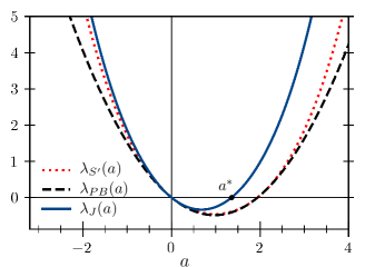
Figure 1: Illustrated definition of the effective affinity $a^{\ast}$. The logarithmic moment generating function $\lambda_{J}$ is plotted as a function of $a$ for an example current $J$ in the four state model of Fig. 2 (see Supplementary Material  [39] for definitions). In addition, the logarithmic moment generating $\lambda_{S^{\prime}}$ for the rescaled fluctuating entropy production $S^{\prime}=S/\dot{s}$ , and the parabola $\lambda_{PB}(a)=a\overline{j}(-1+a\overline{j}/\dot{s})$ that appears on the right hand side of the inequality (13) are plotted as a function of $a$. Notice that in both cases ($J_{t}$ and $S^{\prime}_{t}$) the average current equals $1$.

Obtaining the effective affinity from the tilted generator.

Although it is difficult to determine $\lambda_{J}(a)$ directly from its definition (11), we can readily obtain $\lambda_{J}(a)$, and thus also the effective affinity, from the eigenvalues of a tilted $\mathbf{q}$-matrix. Indeed, applying Kolmogorov’s backward equation to $\langle e^{-aJ_{t}}\rangle$, it follows that $\lambda_{J}(a)$ is the Perron root (i.e., the eigenvalue with the largest real part) of the matrix [36, 40]

$$\tilde{\mathbf{q}}_{xy}(a)=\left\{\begin{array}[]{ccc}\mathbf{q}_{xy}e^{-ac_{xy}},&{\rm if}&x\neq y,\\ -\sum_{z\in\mathcal{X}\setminus\left\{x\right\}}\mathbf{q}_{xz},&{\rm if}&x=y,\end{array}\right.$$ (12)

and $a^{\ast}$ is the value of $a$ for which the Perron root vanishes. Having defined $a^{\ast}$, we continue with deriving the main properties (2) and (3) of the effective affinity.

Lower bound on dissipation.

The bound (2) follows from using the effective affinity definition $\lambda_{J}(a^{\ast})=0$ in the lower bound

$$\lambda_{J}(a)\geq a\overline{j}\left(-1+a\frac{\overline{j}}{\dot{s}}\right),$$ (13)

which follows from the theory of level 2.5 large deviations [41, 42]. Indeed, the parabola on the right-hand side of (13) has the root $a=\dot{s}/\overline{j}$ and according to the inequality (13) this root is larger or equal than $a^{\ast}$.

Martingale associated to $J$.

To derive the law (3) for the infima statistics of currents, we construct a martingale process $M_{t}$ associated with $J_{t}$. A martingale is a stochastic process that satisfies

$$\langle M_{t}|X^{s}_{0}\rangle=M_{s}$$ (14)

for all $s\in[0,t]$, where $\langle\cdot|X^{s}_{0}\rangle$ denotes the expectation conditioned on the trajectory of $X_{t}$ in the interval $[0,s]$. The process

$$M_{t}=\phi_{a^{\ast}}(X_{t})e^{-a^{\ast}J_{t}}$$ (15)

is a martingale, where $\phi_{a}(x)$ is the right eigenvector of $\tilde{\mathbf{q}}(a)$ associated with its Perron root. The martingality of $M_{t}$ follows from the fact that $\phi_{a^{\ast}}(x)e^{-a^{\ast}j}$ is a harmonic function of the generator of the joint process $(X_{t},J_{t})$ (see Supplementary Material [39]).

The martingale $M_{t}$ extends previous results on martingales in stochastic thermodynamics, see Ref. [27] for a review. Notably, for $J_{t}=S_{t}$ we get $M_{t}=\exp(-S_{t})$, as $a^{\ast}=1$ and $\phi=1$, and thus we recover that the exponentiated negative entropy production is a martingale [28, 25], and for $J_{t}=J^{x\rightarrow y}_{t}$ we find the martingale of Ref. [20].

Splitting probability and extreme value statistics.

We derive the infimum law (3) from the martingale $M_{t}$. First, we introduce a related first-passage problem, namely, we consider the first time that the current $J_{t}$ exits the interval $(-\ell_{-},\ell_{+})$, i.e.,

$$T={\rm min}\left\{t\geq 0:J_{t}\notin(-\ell_{-},\ell_{+})\right\}.$$ (16)

This is the gambler’s ruin problem, as introduced by Pascal in the 17th century [43, 44], applied to a fluctuating current $J_{t}$ [45]. The splitting probability $p_{-}$, corresponding with the probability of ruin, is the probability that $J_{T}$ is smaller or equal than $-\ell_{-}$. Using Doob’s optional stopping theorem, $\langle M_{T}\rangle=\langle M_{0}\rangle$ [46] we find that (see Supplementary Material [39])

$$\lim_{\ell_{-}\rightarrow\infty}\frac{|\ln p_{-}|}{\ell_{-}}=a^{\ast}.$$ (17)

Hence, the effective affinity is the exponential decay constant of $p_{-}$. In the limit of $\ell_{+}\rightarrow\infty$, the splitting probability $p_{-}$ is the cumulative distribution of $J_{\rm inf}$, and thus we recover the infimum law (3).

First-passage ratio bound.

The inequality (2) combined with the martingale result (17) implies a trade off relation between dissipation ($\dot{s}$), speed ($\langle T\rangle$), and uncertainty $|\ln p_{-}|$. Indeed, using Eq. (17) and Wald’s equality for fluctuating currents [47, 48],

$$\overline{j}=\frac{\ell_{+}}{\langle T\rangle}(1+o_{\ell_{\rm min}}(1)),$$ (18)

in the inequality (2) yields

$$\dot{s}\geq\frac{\ell_{+}}{\ell_{-}}\frac{|\ln p_{-}|}{\langle T\rangle}\left(1+o_{\ell_{\rm min}}(1)\right),$$ (19)

where $o_{\ell_{\rm min}}(1)$ represents an arbitrary function that decays to zero when $\ell_{\rm min}={\rm min}\left\{\ell_{-},\ell_{+}\right\}$ diverges. Notice that the present derivation of (19) with $M_{t}$ is clearer than the previous derivation in Ref. [29] that uses scaling arguments. In addition, we have shown that the right-hand side of (13) equals $\overline{j}a^{\ast}$, which is an improvement on previous work that estimated the right-hand side via simulations at finite thresholds [49].

Equivalence with the thermodynamic uncertainty relations for Gaussian fluctuations.

The inequality (19) is reminiscent of the thermodynamic uncertainty relations [50, 42, 51], but with the important difference that uncertainty is quantified with the splitting probability $p_{-}$ instead of the variance of $T$ or $J_{t}$. We show that the inequalities (19) and (2) are equivalent with the thermodynamic uncertainty relations when the probability distribution of $J_{t}$ converges asymptotically with time to a Gaussian distribution. Indeed, it holds then that $\lambda_{J}(a)=a(a\sigma^{2}/2-\overline{j})$, where $\sigma$ is the standard deviation of $J_{t}/t$, and thus $a^{\ast}=2\overline{j}/\sigma^{2}$. Substituting this value into (2) yields the thermodynamic uncertainty relation $\dot{s}\geq 2(\overline{j}/\sigma)^{2}$ [50, 42].

Cycle equivalence classes.

Having identified the physical properties of $a^{\ast}$, we partition now the set of fluctuating currents $J_{t}$ into equivalence classes that have the same effective affinity $a^{\ast}$. To this purpose, we rely on Schnakenberg’s network theory  [23, 52] that decomposes currents $\overline{j}$ into linear combinations of the form $\overline{j}=\sum_{\gamma\in\mathcal{C}}c_{\gamma}\overline{j}_{\gamma}$, where $\mathcal{C}$ is a set of fundamental cycles of the graph of admissible transitions, $\overline{j}_{\gamma}$ are the corresponding cycle currents, and $c_{\gamma}$ are the cycle coefficients obtained from summing up the $c_{x,y}$ coefficients along the cycle $\gamma$ (see Supplemental Material [39]). The cycle coefficients $c_{\gamma}$ partition the space $\mathbb{R}^{|\mathcal{E}|}$ of coefficients $c_{x,y}$ into Euclidean spaces of dimension $|\mathcal{X}|-1$ that contain all coefficients $c_{x,y}$ that yield the same cycle coefficients $c_{\gamma}$. We call the corresponding set a cycle equivalence class, and we denote the cycle equivalence class associated with $J_{t}$ by $[J_{t}]$. Importantly, currents that belong to the same cycle equivalence class have the same cumulant generating function $\lambda_{J}(a)$, and hence also the same effective affinity $a^{\ast}$ (see Supplementary Material [39]).

Tightness of the effective affinity bound.

Next, we characterise a set of currents $J_{t}$ that attain the equality in Eq. (2). Consider fluctuating currents that are proportional to the stochastic entropy production $S_{t}$, i.e., $J_{t}=kS_{t}$ with $k\in\mathbb{R}$. Such currents satisfy the Gallavotti-Cohen symmetry [16]

$$\lambda_{J}(a)=\lambda_{J}\left(k^{-1}-a\right),$$ (20)

and thus $a^{\ast}=1/k$. In addition, since $\overline{j}=k\dot{s}$ the equalities in (2) and (19) are attained. Thus, currents that belong to the cycle equivalence classes $[kS_{t}]$ with $k\in\mathbb{R}$ are precise currents in the sense of attaining the equality (19).

Toy model with two fundamental cycles.

Do there exist currents that do not belong to one of the cycle equivalence classes $[kS_{t}]$, but nevertheless attain the equality in (2)? We settle this question for models with two fundamental cycles through a a numerical case study of the four state model illustrated in Fig. 2(a). The four state model has two fundamental cycles denoted by $\gamma=1$ and $\gamma=2$, and hence the cycle equivalence classes of this model are determined by two coefficients $c_{1}$ and $c_{2}$, such that $\overline{j}=c_{1}\overline{j}_{1}+c_{2}\overline{j}_{2}$. We normalise $c_{1}$ and $c_{2}$ such that $\overline{j}=1$. For this choice of normalisation, the dependence of $a^{\ast}$ on the $c_{xy}$-coefficients that define $J_{t}$ is fully determined by one parameter, namely the angle $\alpha$ between the vectors $(c_{1},c_{2})$ and $(a_{1},a_{2})$, where the latter are the cycle coefficients of $[S_{t}/\dot{s}]$; see Fig. 2(b) for an illustration.

Figure 2(c) plots $a^{\ast}$ as a function of $\alpha$ for randomly generated transition rates $\mathbf{q}$. Note that according to the inequality (2), $a^{\ast}/\dot{s}\leq 1$, and the equality $a^{\ast}=\dot{s}$ is attained when $\alpha=0$ or $\alpha=\pi$, corresponding with fluctuating currents that belong to $[S_{t}/\dot{s}]$ or $[-S_{t}/\dot{s}]$, respectively. We observe that the effective affinity is a monotonously decreasing/increasing function between the value of $\alpha$ with vanishing average current (where $a^{\ast}=0$) and the end point values $\alpha=0$ and $\alpha=\pi$. Hence, for the four state model the equality in the trade-off relations (2) and (19) is only attained for currents that belong to the cycle equivalence classes $[kS_{t}]$ with $k\in\mathbb{R}$.

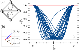
Figure 2: Panel(a): Graph of admissible transitions for the four state model with the two cycles $\gamma=1$ and $\gamma=2$ as indicated. Panel (b): Sketch of cycle affinities $(a_{1},a_{2})$, cycle currents $(j_{1},j_{2})$, and cycle coefficients $(c_{1},c_{2})$ plotted in $\mathbb{R}^{2}$, with the angle $\alpha$ indicated. Panel (c): $a^{\ast}/\dot{s}$ as a function of $\alpha$ for $\overline{j}=1$. Different lines correspond to different choices of the rates $\mathbf{q}_{xy}$, here randomly generated with uniform distribution between $0$ and $1$.

Stalling force interpretation of the effective affinity.

In the special case of edge currents, i.e., $J=J^{xy}$, the effective affinity equals [13, 14],

$$a^{\ast}=\ln\frac{p^{(x,y)}_{\rm ss}(x)\mathbf{q}_{xy}}{p^{(x,y)}_{\rm ss}(y)\mathbf{q}_{yx}}$$ (21)

where $p^{(x,y)}_{\rm ss}(x)$ is the probability mass function of a modified Markov jump process for which the transition rates along the $(x,y)$-edge have been set to zero (see Supplementary Material [39]). Interestingly, as shown in Refs. [13, 14], for edge currents the effective affinity equals the additional force required to stall the current. This means that if we consider a modified process with rates $\tilde{\mathbf{q}}_{xy}/\tilde{\mathbf{q}}_{yx}=\exp(f)\mathbf{q}_{xy}/\mathbf{q}_{yx}$, then at stalling when $\overline{j}=0$ it holds that $f=a^{\ast}$.

The stalling force property of $a^{\ast}$ does not generalise to generic currents. Nevertheless, the effective affinity is a stalling force for currents that belong to $[J^{xy}_{t}]$, as such currents have the same effective affinity as $J^{xy}_{t}$. Note that the equivalence class $[J^{xy}_{t}]$ contains currents that are not edge currents, as we illustrate next in a biophysical model of a molecular motor.

Effective affinity in a mechanochemical model of kinesin-1.

We analyse the effective affinity for the positional current of a molecular motor bound to a one-dimensional substrate. Specifically, we use the mechanochemical model for kinesin-1 from Ref. [53]. In this model, the molecular motor can step forward through multiple biochemical pathways, as shown in Fig. 3(a), and the kinesin-1 steps consist of two substeps, consistent with experimental data [54, 55]. Therefore, the positional current sums up contributions from multiple edges, viz., the edges $(1,3)$, $(4,2)$ and $(2,3)$ (see Supplementary Material [39] for details). Nevertheless, the positional current $J$ in this biophysical model belongs to $[J^{23}_{t}]$, and hence the stalling force property holds.

Since the selected current is a displacement, the effective affinity has the same dimensions as a mechanical force. In the present model, this is more than a dimensional analogy, as the effective affinity equals the additional force required to stall the molecular motor, i.e., $a^{\ast}=f_{0}-f$, where $f$ is the mechanical force opposing forward motion and $f_{0}$ is the value of $f$ for which the motor stalls. Indeed, as shown in Fig. 3(b), $a^{\ast}$ decreases linearly as a function of $f$ with slope equal to $-1$, and by definition $a^{\ast}$ vanishes when the positional current $\overline{j}$ vanishes.

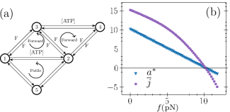
Figure 3: (a)Graph of admissible transitions in a mechanochemical model of kinesin-1 [53], which includes three cycles, two corresponding with forward motion and one futile cycle. The dependence of the rates on the mechanical force $f$ and the ATP concentration are indicated. (b) The average positional current $\overline{j}$ and effective affinity $a^{\ast}$ as a function of $f$. See Supplementary Material [39] for the model parameters used.

Discussion.

We have introduced the concept of an effective affinity for a generic current, which is a unique real number associated with currents in Markov processes that quantifies several physical properties of fluctuating currents. Notably, the effective affinity multiplied by the average current lower bounds dissipation, see Eq. (2) and the effective affinity is the exponential decay constant that characterises the tails of the infimum statistics of the current, see Eq. (3). In addition, since the effective affinity is a generalisation of the edge affinity from Refs. [13, 14] it admits, under certain physical conditions that we specified here, a stalling force interpretation.

In mathematical models, the effective affinity can readily be computed from the tilted generator $\tilde{\mathbf{q}}$. Getting estimates of effective affinities in experimental systems, such as molecular motors, is more challenging, but certainly not out of reach. For example, the extreme value statistics formula (3) can be used to estimate $a^{\ast}$, and we have shown that in a biophysical model of a kinesin-1 motor the effective affinity can be estimated from the motor’s stalling force.

From a methodological point of view, this Letter introduces a new class of martingales, $M_{t}$, associated to generic currents, which extends previous work on entropy production [28, 25, 26] and single edge currents [20]. Given the numerous properties of martingales, as outlined in [27], the $M_{t}$ add to existing techniques for studying current fluctuations.