single = false, list/sort = true, cite/group = true, cite/group/cmd = cite/group/pre = , \DeclareAcronymprf short = PRF, long = Pixel Response Function \DeclareAcronympsf short = PSF, long = point spread function, \DeclareAcronymgpu short = GPU, long = Graphics Processing Unit \DeclareAcronymfim short = FIM, long = Fisher Information Matrix, cite = fisher1925 \DeclareAcronymhmc short = HMC, long = Hamiltonian Monte Carlo, cite = Betancourt2017 \DeclareAcronymmcmc short = MCMC, long = Markov Chain Monte Carlo, cite = Metropolis1953 \DeclareAcronymgp short = GP, long = Gaussian Process, cite = Rasmussen2005,Aigrain2022 \DeclareAcronymcrlb short = CRLB, long = Cramér-Rao Lower Bound, cite = rao1945,cramer1947 \DeclareAcronymsnr short = SNR, long = signal-to-noise ratio \DeclareAcronympld short = PLD, long = Pixel Level Decorrelation, cite = everest \DeclareAcronymk2sff short = SFF, long = Self Flat-Fielding, cite = self_flat-fielding \DeclareAcronymcpm short = CPM, long = Causal Pixel Model, cite = causal_pixel \DeclareAcronymapfwfs short = APF-WFS, long = Asymmetric Pupil Fourier Wavefront Sensor, cite = Martinache2013,Martinache2016 \DeclareAcronymapi short = API, long = Application Programming Interface \DeclareAcronymjit short = jit, long = Just-In-Time \DeclareAcronymhpc short = HPC, long = High-Performance Computing \DeclareAcronymopd short = OPD, long = Optical Path Difference \DeclareAcronymmle short = MLE, long = maximum-likelihood estimate
Differentiable Optics with Lux II: Optical Design Maximizing Fisher Information
Abstract
The design of astronomical hardware operating at the diffraction limit requires optimization of physical optical simulations of the instrument with respect to desired figures of merit, such as throughput or astrometric accuracy. These systems can be high dimensional, with highly nonlinear relationships between outputs and the adjustable parameters of the hardware. In this series of papers we present and apply Lux, an open-source end-to-end differentiable optical modelling framework. Automatic differentiation enables not just efficient high-dimensional optimization of astronomical hardware designs, but also Bayesian experimental design directly targeting the precision of experimental outcomes. Automatic second derivatives enable the exact and numerically stable calculation of parameter covariance forecasts, and higher derivatives of these enable direct optimization of these forecasts. We validate this method against analytic theory and illustrate its utility in evaluating the astrometric precision of a parametrized telescope model, and the design of a diffractive pupil to achieve optimal astrometric performance for exoplanet searches. The source code and tutorial software are open source and publicly available, targeting researchers who may wish to harness Lux for their own optical simulation problems.
Send correspondence to L. Desdoigts:
E-mail: \linkablelouis.desdoigts@sydney.edu.au
Differentiable Optics with Lux: II - Informational Optical Design
Keywords: optics, detectors, phase retrieval, simulations, diffractive optics
1 Introduction
Advances in contemporary observational astronomy are driven by progress in instrumentation and hardware, enabling measurements with improved sensitivity and lower noise. This is particularly true for exoplanetary science where signals can be many orders of magnitude smaller than the noise, and it is essential to accurately model the pattern, or \acpsf, by which starlight is spread out on the detector, and to engineer hardware to achieve favourable \acppsf. For example apodizing phase plate coronagraphs [1] engineer spatially-varying \acppsf that suppress light within a defined field for on-axis sources through transformations to the wavefront in multiple conjugate planes, thereby revealing dim objects otherwise hidden within the glare. This is achieved with an apodizing phase plate [2], a phase mask placed in a telescope pupil plane that reshapes the \acpsf, the design of which poses nonlinear optimisation challenges [3]. Astrometric exoplanetary detection [4] similarly requires careful consideration of instrumental design such that \acppsf are stable and can be used to characterise the time-varying instrumental imperfections, achieving measurement precisions required for tiny (micro-arcsecond) signals. This can be achieved with widefield space-based surveys such as Gaia, or with smaller telescopes and diffractive pupils that engineer \acppsf with favourable properties [5, 6]. In either case and elsewhere in astrometry we require great stability and precise data-driven calibration of diffraction effects in the \acpsf.
Advances in software and algorithms are therefore essential for both data analysis and to facilitate hardware design. A range of open-source physical optics simulation codes [7, 8, 9] have been developed to model imaging systems end to end, and design and data analysis problems might optimize or sample from such models with grid-based or \acmcmc methods. For models with many parameters (and this is easy to achieve by considering many modes of phase aberration, multiple sources in the field of view, without even considering pixel by pixel effects on the detector) these can be impossible to reliably sample or optimize [11] unless it is also possible to evaluate not just the value but also the gradient of the objective function. Algorithms for automatic differentiation or ‘autodiff’[12] are the foundational technology used in artificial intelligence and machine learning [13], and increasingly important in software for the physical sciences. Autodiff makes it possible to evaluate the partial derivatives of an appropriately written computer program’s floating-point outputs with respect to floating-point arguments. Through repeated applications of the chain rule, autodiff delivers exact derivatives with complexity that scales with the computational cost of the model, not with its number of parameters. Considerable industry and academic effort has gone into developing performant and user-friendly numerical software libraries with autodiff capability: PyTorch [14], TensorFlow [15], Julia [16], or our preferred library used in this work, Jax [17]. These abstract the details of code differentiation from the user, so that it is possible to construct gradients and even higher-order and higher-dimensional derivatives of functions without, in most cases, requiring explicit human engagement with the underlying mathematics.
Differentiable forward models in physics permit optimization and inference with very many parameters, and to incorporate flexible nonparametric models [18] jointly with deterministic physics. Autodiff has been used recently in optical and imaging science for phase retrieval and \acpsf modelling [19, 20, 21, 22]. In the first paper in this series [23], we presented Lux: an open-source physical optics model, designed to tackle problems across optics. Built in Python with Jax, Lux features autodiff, ‘just-in-time’ compiling for hardware acceleration, higher-order derivatives, and natively deploys on \acpgpu and \achpc environments. We applied Lux to perform end-to-end phase retrieval and detector calibration directly from realistic simulated imaging data.
This manuscript builds on this previous work, exploring how numerically stable higher-order gradients permit the calculation of covariance and Fisher matrices [24, 25] under a multivariate normal posterior approximation. By constructing differentiable optical models we can differentiate a likelihood function with respect to any astrophysical or instrumental model parameters to compute covariance matrices. This enables Fisher forecasting, a statistical technique used to estimate the precision of parameter estimates from a future experiment, and enables computation of the covariance matrix. The covariance matrix obtained thus gives us the \accrlb – the information-theoretical limit on parameter constraints achievable with an experiment. This is a common approach for the planning of new instruments and surveys in cosmology; for example, forecasting how well observations of the cosmic microwave background [28] or spectroscopic surveys [29] will constrain bulk cosmological parameters, under the choice of settings in a preliminary instrument design and marginalized over nuisance parameters.
The ability to calculate these Fisher matrices using autodiff then enables Bayesian experimental design[30, 31, 32] via gradient descent. This might involve optimizing the uncertainty of a particular parameter, or a norm such as the determinant or trace of the \accrlb. In Section 2 of this Paper we briefly describe the underlying theory, and in Section 3 we validate calculations made with Lux against analytic theory. We apply this in Section 4 to optimize the design of a phase mask for the astrometric mission Toliman [6], a small telescope aiming to detect planets around Cen AB by measuring micro-arcsecond perturbations in the relative binary positions.
2 Fisher Information and Bayesian Experimental Design
The key feature of autodiff exploited in this Paper is the ability to efficiently calculate a multivariate normal approximation to a probability distribution. Consider an imaging system and sources, parametrized by , that generate data . In solving an inverse problem, we want to infer given and any prior information. We can use Bayes’ rule to update our prior knowledge of conditioned on our prior knowledge given :
| (1) |
It is more convenient computationally to express this in logarithmic units,
| (2) |
At the maximum likelihood, the score – the gradient of the log-likelihood with respect to the parameters – vanishes, and is the \acmle of these parameters . We may then be motivated to consider a Taylor expansion of about this point, dropping the prior 111We can do so without loss of generality; to include the prior, we can replace throughout this calculation with instead., to estimate the distribution near the maximum. Going up to second-order is equivalent to approximating as a multivariate normal – Laplace’s Method [33, 34]:
| (3) |
As we can see, the Hessian of is the \acfim,
| (4) |
formally defined as the variance of the score. The parameter covariance matrix is calculated as the negative inverse of the \acfim
| (5) |
and fully describes the best-fit multivariate normal - a reasonable estimate of the behaviour of a likelihood distribution around its peak.
The \acfim has some convenient properties [36], firstly the Fisher matrices for two independent experiments add () allowing for the \acfim to be calculated independently for any observations that add linearly, such as dithered images. Secondly, since parameter marginalisation happens through the matrix inversion of , row and column can be deleted from in order to remove its contribution to the resulting covaraince matrix. Importantly, the covariance matrix of a model with parameters calculated using the observation produced by that model given parameters is the \accrlb: the lower bound on the variance of an unbiased frequentist estimator of . It is not possible to recover parameters better than the \accrlb, and so it is useful for forecasting the sensitivity of an experiment to the parameters of a model under consideration, irrespective of how data analysis will be carried out.
In the remainder of this paper, we will assume that the multivariate normal approximation to our likelihood holds, and that the Fisher and covariance matrix calculated from this Hessian is accurate. We also assume that our measurements are photon-noise dominated and therefore exclusively use a Poissonian likelihood throughout the rest of the work. Furthermore, all calculations of and references to the covariance matrix are of the parameter covariance matrix, calculated against simulated data without noise realisations, therefore completely describing the \accrlb under the Laplace approximation which is already assumed valid.
3 Comparison to Theory
In especially simple cases, the Fisher forecast of parameters of interest can be obtained by analytic theory. In this Section we validate the autodiff method against parameter uncertainties calculated via the Laplace method to an analytic expression derived under a series of simplifying assumptions allowing a closed form solution, as well as those output by a \achmc algorithm. We start with an illustrative toy problem: obtaining a position measurement from the image plane of a simple telescope. Given a circular pupil support and a monochromatic point source, the \acpsf is the well known Airy disk and the source localization precision of an optical system as a function of photon count is given by
| (6) |
where is the radial uncertaintly in the positional measurement, is the number of photons, is the wavelength of light and is the diameter of the aperture [5]. We can use this analytic equation and the values calculated using the Laplace methods described in Section 3 and compare them to the results of the \achmc, shown in Figure 1. We assume that the signal is photon noise limited, and therefore choose a per-pixel Poisson distribution as the likelihood function for both the Laplace and HMC methods, which is the same used to derive Equation 6.
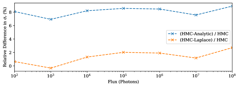
Analytically derived values like Equation 6 are a useful ‘rule of thumb’ estimate of true performance, but can not be used to understand the effects of various real-world complexities. As shown in Figure 1 the analytic values give a consistent overestimate of system performance as it is unable to account for the loss of information consequential to only measuring a finite portion of the image plane on a pixelised grid. The numerical Laplace and \achmc methods directly include this effect in the model, simulating not an ideal and infinite \acpsf, but one with realistic pixel sampling and field of view, giving closely similar answers that differ slightly from the analytic values. A real imaging system is in general broadband and chromatic, with imperfect surfaces, secondary mirror spiders, all of which directly influence the \acppsf and can in general only be modelled numerically. In these cases, with a differentiable forward model the covariance forecast is simply a one-line call to evaluate the Hessian.
4 Optical Design
Not only can the covariance matrix be evaluated at given parameter values, but also the higher-order gradients delivered by the Jax framework enable differentiation and therefore optimisation of the covariance matrix itself. This opens up the possibility of Bayesian experimental design, allowing for gradient descent directly on properties and functions of the covariance matrix such as the entropy, marginalised variances, or as we show in this example, individual components of the covariance matrix marginalised over the rest of the model. As with the rest of this work presented, this requires only a forward model of the system in a differentiable framework.
The application chosen is the design of the diffractive pupil required for the Toliman mission [6], a small space telescope which aims to measure the micro-arcsecond scale angular perturbation induced on the host star by the orbital gravitational reflex motion from an (unseen) low-mass planet. Such a formidable challenge requires the engineering of a \acpsf that maximally encodes both instrument meteorology and scientific signals of interest. The solution to these challenges incorporates a binary-valued diffractive pupil and a spectrometer, all integrated into the \acpsf of the telescope by engraving phase patterns onto the entrance pupil. Specifically crossed sinusoidal patterns are used to produce a spectrometer, which are written on top of the primary diffractive pupil pattern which enables the optical metrology and astrometric science measurement. The latter pattern consists of regions of zero/ phase which are separated by sharp transitional boundaries. This pattern is required to be binary as a primary design constraint of the Toliman diffractive pupil. The detailed chain of optical signal encoding together with recovery of contemporaneous system state metrology, as devised for this mission, is quite complex. Its inclusion here is a an ideal exemplar for the methods developed in this work: it is not essential for the reader to understand all the reasons for the design drivers and figures of metric that underpin the project.
Here, we take the design of the Toliman diffractive pupil as the most complex demonstration of analysis by our autodiff frameworks. In approaching the optimisation problem, the required metrics can then be summarised: find a binary-valued diffractive pupil that maximally constrains the relative separation of a binary star , marginalised over the remaining astrophysical parameters: mean position in arcseconds, position angle in degrees, total flux in photons, dimensionless contrast as the ratio of the component fluxes, mean wavelength in nm, as well as the following optical parameters: pixel scale in arcsec/pixel and optical aberrations modelled as a sum of normalized Zernike polynomials with coefficients in nm.
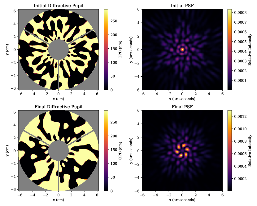
The requirement for binary phases presents a challenge for gradient-based optimisation methods as the distribution is inherently discontinuous. In order to avoid this problem of discrete-optimisation for the values of the pupil we instead use the CLIMB algorithm [20] in order to differentiably map a continuous set of basis vectors onto a single array with only binary values, except at the boundary between those regions. We built a basis from a set of log harmonic radial functions and radial sine and cosine functions as found in previous work [20]We can choose any arbitrary set of basis vectors, however one should leverage the knowledge of their particular problem to inform their choice. In this case we use basis vectors with three-fold rotational symmetry as this naturally improves sensitivity to even-mode Zernike aberrations. Ultimately the choice of basis vectors is somewhat arbitrary as these methods allow for basis vectors to be swapped at no cost to the user.
We construct a polychromatic model of the Toliman optical system with a clear aperture of 125 mm over the full bandpass of 530-640 nm sampled at three uniformly spaced wavelength with a pixel scale of 0.375 arcseconds per pixel, Nyquist. We then model the expected signals from the binary star Centauri AB at the projected separation of 10 arcseconds at the proposed time of mission launch in the mid 2020’s.
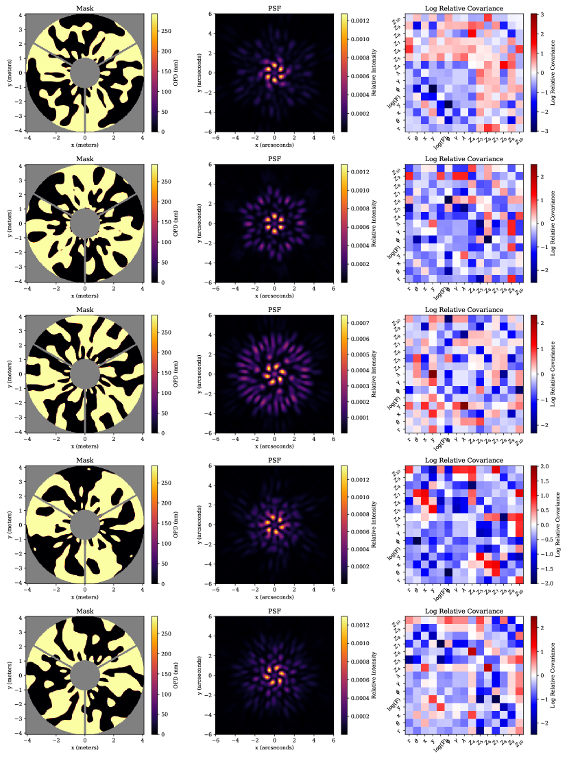
Our loss function involves first calculation of the covariance matrix of this complex forward model, using a per-pixel Poisson likelihood function under the assumption of being photon noise limited, and then selecting out the binary separation variance component, which we seek to minimise. We calculate the gradient of this loss function with respect to the basis vector coefficients in the diffractive pupil in order to optimise them with respect to the entire model, and applied 50 epochs of the Adam [38] optimiser. This optimisation process is only able to find the local minima around the the initial parameters, therefore this design process was repeated for a total of 5 random initialisation seeds, with Figure 6 in the appendix depicting the final pupils obtained with its associated \acpsf and relative covariance matrix i.e. . We do not analyse the performance differences between the post optimised pupils as this is only a methodological demonstration.
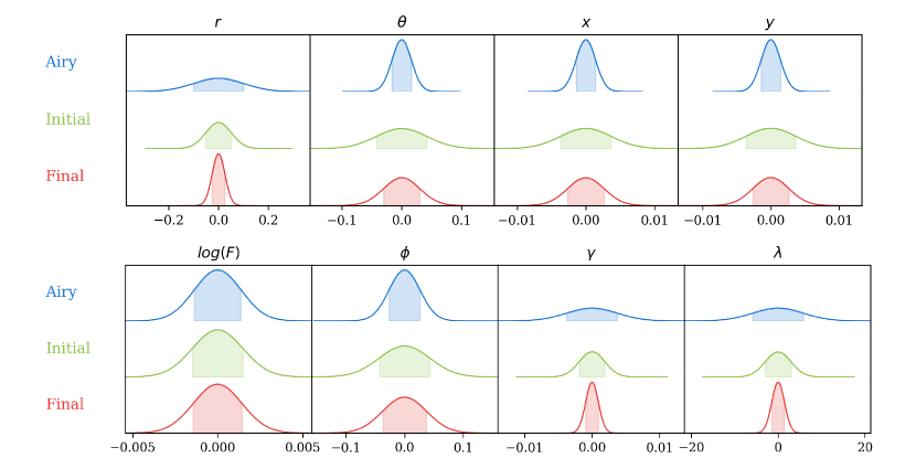
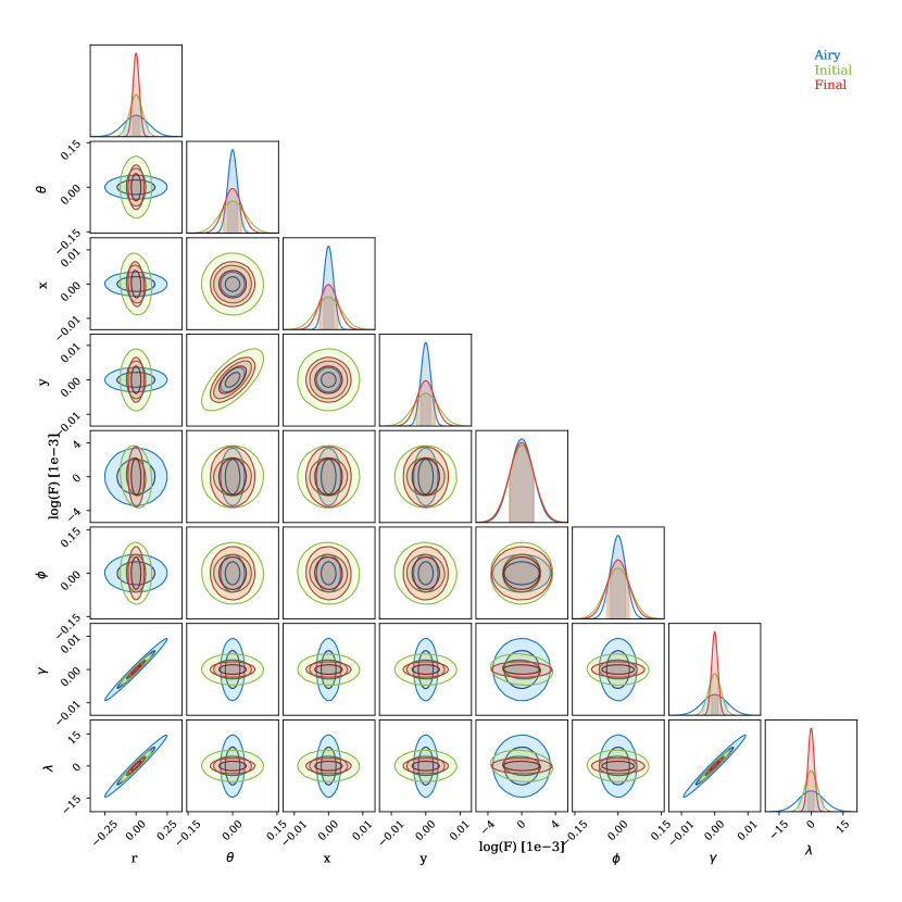
The initial and final pupil-\acpsf pairs are shown in Figure 2, where we can see that the final \acpsf is concentrated into a small number of brighter peaks near the center, plus a series of dimmer peaks surrounding it. Figure 3 shows the parameter posteriors for both the initial and final pupils, as well as an optical system with a clear pupil producing an Airy-disk like \acpsf as a benchmark. We see the greatest improvement for the optimisation metric, the binary separation , as well as the pixel scale and mean wavelength . The full corner plot is shown in Figure 5. Note that the optical aberrations have been omitted from these plots for visualisation purposes, although they were present for the optimisation and have been marginalised over.
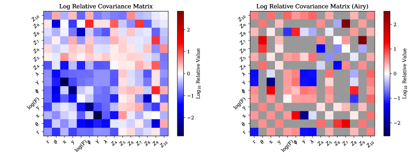
Interestingly, the pre-optimisation model outperforms the Airy system, implying a good choice of basis vectors for the diffractive pupil. Despite the improved performance in the binary separation metric, the diffractive pupil model is inferior in recovery of both the (x, y) position and position angle . Figure 4 compares the full performance of these models to each other by visualising their relative covariance matrices. This Figure reveals some interesting properties of this optimisation process, we can see that while most elements of the covariance matrix show improved performance, some end with degraded performance. This is explained through the marginalisation process inherent when inverting fisher matrices to get covariance matrices - parameters with little to no covariance with the parameter of interest can have degraded performance, allowing improved performance of those that do. This results in an optimisation process that is fully coherent of the complex relationships between different parameters within a system. The pupil mask design approach here offers a significant improvement in the astrometric performance of Toliman and will form the basis of its eventual hardware implementation.
5 Discussion
This manuscript has followed a tutorial approach built upon a concrete example to illustrate the use of these autodiff enabled Fisher Information methods. First laying out the theory and validating the appropriate conditions required, we explored how overall performance of complex system can be analysed, and furthermore used to optimise instrumental components. We did not examine the effect of priors instead (for clarity) choosing example problems that did not require them. Inclusion of simple multivariate normal priors would be trivial as Fisher information is additive.
The methods to calculate Fisher Information presented in this work provide a simple and straightforward way to explore, analyse and optimise models, however it is important to be cognisant of limitations. Firstly the Laplace approximation assumes that all posteriors are multivariate normal about the maximum likelihood estimate. This assumption will not hold in a general sense for systems with complex parameter degeneracies. While an understanding of the local topology of the posterior about the maximum likelihood estimate can be found, this can not function as a general replacement for sampling of the posteriors via Monte Carlo methods which serve to understand the global topology of the posterior. However, many problems either have posteriors that can adequately be represented by a multivariate normal, or else do not require a global understanding of the posterior and hence can be solved using the second order approximation provided by the Laplace assumption.
6 Conclusion
Advances in astronomical sciences hinge on both improved hardware and observational platforms, and also software innovations contributing to superior hardware design and data analysis. The field of exoplanetary science with noisy signals that demand meticulous calibration and characterisation place some of the most demanding requirements on both instrumental design and data inference. Autodiff has already proven capable of advancing astrophysical measurements and calibration techniques [22], however the field lacks a generalised frameworks for differentiable optics; a gap which Lux has been designed to fill.
In this manuscript we have explored new avenues for analysis and design of optical systems harnessing the stable calculation of Fisher matrices using autodiff. This method is in agreement with analytically derived expressions when examined under the correct assumptions and furthermore, can be used to explore extensions to a more relaxed set of assumptions. These methods provide new ways to probe the way different instrumental architectures affects the recovery of science goals, and straightforward algorithms for optimal experimental design to constrain astrophysical parameters without detailed pen-and-paper analysis. A differentiable forward model allows covariance matrices to be calculated directly using different instrumental configurations for comparison, or individual components can be optimised directly either on individual components of the covariance matrix, its properties, or norms.
These differentiable methods allow inference of more complex posteriors. Stochastic variational inference [39] enables parameter degeneracies resulting in non-Gaussian posteriors to be approximated by minimising the divergence between the inferred and true posterior. Extending this, automatic differentiation variation inference [40] utilises the derivatives of a model to explore the posterior parameter space more efficiently, and can be applied directly to differentiable optical models in order to address unavoidable parameter degeneracies present in complex data sets.
The principled methods of calculating the Fisher information through complex instrumentation laid out in this work suggests new approaches, not only for understanding existing data, but also for the design of future instrumentation with statistically principled optimisation. As one particularly promising use case, future coronagraphic instrument design based on autodiff may be made more robust to realistic noise processes such as low-order wavefront error [41] or the low wind effect [42]. With these tools, novel architectures can be rapidly explored and optimised with respect to evidence ratios, robustness to optical aberrations, or spectral parameter estimation. The same principles can be applied to other instruments such as spectrographs for radial velocity planet detection, enabling joint end-to-end optimisation of optical systems and observational regimes.
7 Code, Data, and Materials
As part of our commitment to open science, we have released Lux as an open source package under a BSD three-clause at github.com/LouisDesdoigts/dLux. Furthermore an accompanying Jupyter notebook that produces all results and figures in this paper is publicly hosted at github.com/LouisDesdoigts/FIM_tutorial. We encourage readers to replicate our work and apply the methods presented in this manuscript to their own problems.
Acknowledgements
We acknowledge and pay respect to the traditional owners of the land on which the University of Queensland and the University of Sydney are situated, upon whose unceded, sovereign, ancestral lands we work. We pay respects to their Ancestors and descendants, who continue cultural and spiritual connections to Country.
References
- [1] O. Guyon, E. A. Pluzhnik, M. J. Kuchner, B. Collins, and S. T. Ridgway, “Theoretical Limits on Extrasolar Terrestrial Planet Detection with Coronagraphs,” ApJS 167, pp. 81–99, Nov. 2006.
- [2] J. L. Codona, M. A. Kenworthy, P. M. Hinz, J. R. P. Angel, and N. J. Woolf, “A high-contrast coronagraph for the MMT using phase apodization: design and observations at 5 microns and 2 /D radius,” in Society of Photo-Optical Instrumentation Engineers (SPIE) Conference Series, I. S. McLean and M. Iye, eds., Society of Photo-Optical Instrumentation Engineers (SPIE) Conference Series 6269, p. 62691N, June 2006.
- [3] E. H. Por, “Optimal design of apodizing phase plate coronagraphs,” in Techniques and Instrumentation for Detection of Exoplanets VIII, S. Shaklan, ed., 10400, pp. 236 – 247, International Society for Optics and Photonics, SPIE, 2017.
- [4] A. Sozzetti, “Astrometric Methods and Instrumentation to Identify and Characterize Extrasolar Planets: A Review,” PASP 117, pp. 1021–1048, Oct. 2005.
- [5] O. Guyon, E. A. Bendek, J. A. Eisner, R. Angel, N. J. Woolf, T. D. Milster, S. M. Ammons, M. Shao, S. Shaklan, M. Levine, B. Nemati, J. Pitman, R. A. Woodruff, and R. Belikov, “High-precision Astrometry with a Diffractive Pupil Telescope,” ApJS 200, p. 11, June 2012.
- [6] P. Tuthill, E. Bendek, O. Guyon, A. Horton, B. Jeffries, N. Jovanovic, P. Klupar, K. Larkin, B. Norris, B. Pope, and M. Shao, “The TOLIMAN space telescope,” in Optical and Infrared Interferometry and Imaging VI, M. J. Creech-Eakman, P. G. Tuthill, and A. Mérand, eds., 10701, pp. 432 – 441, International Society for Optics and Photonics, SPIE, 2018.
- [7] M. D. Perrin, R. Soummer, E. M. Elliott, M. D. Lallo, and A. Sivaramakrishnan, Simulating point spread functions for the James Webb Space Telescope with WebbPSF, vol. 8442 of Society of Photo-Optical Instrumentation Engineers (SPIE) Conference Series, p. 84423D. 2012.
- [8] B. Dube, “prysm: A python optics module,” Journal of Open Source Software 4(37), p. 1352, 2019.
- [9] E. H. Por, S. Y. Haffert, V. M. Radhakrishnan, D. S. Doelman, M. Van Kooten, and S. P. Bos, “High Contrast Imaging for Python (HCIPy): an open-source adaptive optics and coronagraph simulator,” in Adaptive Optics Systems VI, Proc. SPIE 10703, 2018.
- [10] N. Metropolis, A. W. Rosenbluth, M. N. Rosenbluth, A. H. Teller, and E. Teller, “Equation of state calculations by fast computing machines,” The Journal of Chemical Physics 21, pp. 1087–1092, June 1953.
- [11] D. Huijser, J. Goodman, and B. J. Brewer, “Properties of the affine-invariant ensemble sampler's ‘stretch move’ in high dimensions,” Australian & New Zealand Journal of Statistics 64, pp. 1–26, Feb. 2022.
- [12] C. C. Margossian, “A Review of automatic differentiation and its efficient implementation,” arXiv e-prints , p. arXiv:1811.05031, Nov. 2018.
- [13] Y. LeCun, Y. Bengio, and G. Hinton, “Deep learning,” Nature 521, pp. 436–444, May 2015.
- [14] A. Paszke, S. Gross, F. Massa, A. Lerer, J. Bradbury, G. Chanan, T. Killeen, Z. Lin, N. Gimelshein, L. Antiga, A. Desmaison, A. Köpf, E. Yang, Z. DeVito, M. Raison, A. Tejani, S. Chilamkurthy, B. Steiner, L. Fang, J. Bai, and S. Chintala, “PyTorch: An Imperative Style, High-Performance Deep Learning Library,” arXiv e-prints , p. arXiv:1912.01703, Dec. 2019.
- [15] M. Abadi, A. Agarwal, P. Barham, E. Brevdo, Z. Chen, C. Citro, G. S. Corrado, A. Davis, J. Dean, M. Devin, S. Ghemawat, I. Goodfellow, A. Harp, G. Irving, M. Isard, Y. Jia, R. Jozefowicz, L. Kaiser, M. Kudlur, J. Levenberg, D. Mané, R. Monga, S. Moore, D. Murray, C. Olah, M. Schuster, J. Shlens, B. Steiner, I. Sutskever, K. Talwar, P. Tucker, V. Vanhoucke, V. Vasudevan, F. Viégas, O. Vinyals, P. Warden, M. Wattenberg, M. Wicke, Y. Yu, and X. Zheng, “TensorFlow: Large-scale machine learning on heterogeneous systems,” 2015. Software available from tensorflow.org.
- [16] J. Bezanson, S. Karpinski, V. B. Shah, and A. Edelman, “Julia: A Fast Dynamic Language for Technical Computing,” arXiv e-prints , p. arXiv:1209.5145, Sep 2012.
- [17] J. Bradbury, R. Frostig, P. Hawkins, M. J. Johnson, C. Leary, D. Maclaurin, and S. Wanderman-Milne, “JAX: composable transformations of Python+NumPy programs,” 2018.
- [18] A. Lavin, D. Krakauer, H. Zenil, J. Gottschlich, T. Mattson, J. Brehmer, A. Anandkumar, S. Choudry, K. Rocki, A. G. Baydin, C. Prunkl, B. Paige, O. Isayev, E. Peterson, P. L. McMahon, J. Macke, K. Cranmer, J. Zhang, H. Wainwright, A. Hanuka, M. Veloso, S. Assefa, S. Zheng, and A. Pfeffer, “Simulation intelligence: Towards a new generation of scientific methods,” 2022.
- [19] A. S. Jurling and J. R. Fienup, “Applications of algorithmic differentiation to phase retrieval algorithms,” J. Opt. Soc. Am. A 31, pp. 1348–1359, Jul 2014.
- [20] A. Wong, B. Pope, L. Desdoigts, P. Tuthill, B. Norris, and C. Betters, “Phase retrieval and design with automatic differentiation: tutorial,” Journal of the Optical Society of America B 38, p. 2465, Aug 2021.
- [21] T. Liaudat, J.-L. Starck, M. Kilbinger, and P.-A. Frugier, “Rethinking the modeling of the instrumental response of telescopes with a differentiable optical model,” arXiv e-prints , p. arXiv:2111.12541, Nov. 2021.
- [22] T. Liaudat, J.-L. Starck, M. Kilbinger, and P.-A. Frugier, “Rethinking data-driven point spread function modeling with a differentiable optical model,” Inverse Problems 39, p. 035008, Mar. 2023.
- [23] L. Desdoigts, B. J. S. Pope, J. Dennis, and P. G. Tuthill, “Differentiable optics with lux: I—deep calibration of flat field and phase retrieval with automatic differentiation,” Journal of Astronomical Telescopes, Instruments, and Systems 9, June 2023.
- [24] N. Bhandari, C. D. Leonard, M. M. Rau, and R. Mandelbaum, “Fisher Matrix Stability,” arXiv e-prints , p. arXiv:2101.00298, Jan. 2021.
- [25] W. R. Coulton and B. D. Wandelt, “How to estimate Fisher matrices from simulations,” arXiv e-prints , p. arXiv:2305.08994, May 2023.
- [26] C. Radhakrishna Rao, “Information and the accuracy attainable in the estimation of statistical parameters,” Bull. Calcutta Math. Soc. 37, pp. 81–91, 1945.
- [27] H. Cramér, “Mathematical methods of statistics,” 1947.
- [28] H. Liu and E. F. Bunn, “Fisher matrix optimization of cosmic microwave background interferometers,” Phys. Rev. D 93, p. 023512, Jan. 2016.
- [29] W. d’Assignies D, C. Zhao, J. Yu, and J.-P. Kneib, “Cosmological Fisher forecasts for next-generation spectroscopic surveys,” MNRAS 521, pp. 3648–3662, May 2023.
- [30] V. Fedorov, Theory of Optimal Experiments, Cellular Neurobiology, Academic Press, 1972.
- [31] K. Chaloner and I. Verdinelli, “Bayesian experimental design: A review,” Statistical Science 10(3), pp. 273–304, 1995.
- [32] E. Ryan, C. Drovandi, J. McGree, and A. Pettitt, “Fully bayesian optimal experimental design: A review,” International Statistical Review 84, pp. 128–154, 2016.
- [33] R. Kass, L. Tierney, and J. Kadane, “Laplace’s method in bayesian analysis,” 1991.
- [34] D. J. C. MacKay, Information Theory, Inference & Learning Algorithms, Cambridge University Press, USA, 2002.
- [35] R. A. Fisher, “Theory of statistical estimation,” Mathematical Proceedings of the Cambridge Philosophical Society 22(5), p. 700–725, 1925.
- [36] D. Coe, “Fisher Matrices and Confidence Ellipses: A Quick-Start Guide and Software,” arXiv e-prints , p. arXiv:0906.4123, June 2009.
- [37] M. Betancourt, “A Conceptual Introduction to Hamiltonian Monte Carlo,” arXiv e-prints , p. arXiv:1701.02434, Jan. 2017.
- [38] D. P. Kingma and J. Ba, “Adam: A method for stochastic optimization,” 2017.
- [39] M. Hoffman, D. M. Blei, C. Wang, and J. Paisley, “Stochastic variational inference,” 2013.
- [40] A. Kucukelbir, D. Tran, R. Ranganath, A. Gelman, and D. M. Blei, “Automatic differentiation variational inference,” 2016.
- [41] T. Currie, N. J. Kasdin, T. D. Groff, J. Lozi, N. Jovanovic, O. Guyon, T. Brandt, F. Martinache, J. Chilcote, N. Skaf, J. Kuhn, P. Pathak, and T. Kudo, “Laboratory and On-sky Validation of the Shaped Pupil Coronagraph’s Sensitivity to Low-order Aberrations With Active Wavefront Control,” PASP 130, p. 044505, Apr. 2018.
- [42] J. Milli, M. Kasper, P. Bourget, C. Pannetier, D. Mouillet, J. F. Sauvage, C. Reyes, T. Fusco, F. Cantalloube, K. Tristam, Z. Wahhaj, J. L. Beuzit, J. H. Girard, D. Mawet, A. Telle, A. Vigan, and M. N’Diaye, “Low wind effect on VLT/SPHERE: impact, mitigation strategy, and results,” in Adaptive Optics Systems VI, L. M. Close, L. Schreiber, and D. Schmidt, eds., Society of Photo-Optical Instrumentation Engineers (SPIE) Conference Series 10703, p. 107032A, July 2018.
- [43] C. R. Harris, K. J. Millman, S. J. van der Walt, R. Gommers, P. Virtanen, D. Cournapeau, E. Wieser, J. Taylor, S. Berg, N. J. Smith, R. Kern, M. Picus, S. Hoyer, M. H. van Kerkwijk, M. Brett, A. Haldane, J. F. del Río, M. Wiebe, P. Peterson, P. Gérard-Marchant, K. Sheppard, T. Reddy, W. Weckesser, H. Abbasi, C. Gohlke, and T. E. Oliphant, “Array programming with NumPy,” Nature 585(7825), pp. 357–362, 2020.
- [44] J. D. Hunter, “Matplotlib: A 2d graphics environment,” Computing In Science & Engineering 9(3), pp. 90–95, 2007.
- [45] D. Phan, N. Pradhan, and M. Jankowiak, “Composable Effects for Flexible and Accelerated Probabilistic Programming in NumPyro,” arXiv e-prints , p. arXiv:1912.11554, Dec. 2019.
- [46] P. Kidger and C. Garcia, “Equinox: neural networks in JAX via callable PyTrees and filtered transformations,” Differentiable Programming workshop at Neural Information Processing Systems 2021 , 2021.
- [47] M. Hessel, D. Budden, F. Viola, M. Rosca, E. Sezener, and T. Hennigan, “Optax: composable gradient transformation and optimisation, in jax!,” 2020.
- [48] S. R. Hinton, “ChainConsumer,” The Journal of Open Source Software 1, p. 00045, Aug. 2016.