Variational Bayes Inference for Spatial Error Models with Missing Data

Anjana Wijayawardhana Corresponding author: anjanaw@uow.edu.au School of Mathematics and Applied Statistics, University of Wollongong, Wollongong, NSW, Australia 0000-0003-3847-2671 David Gunawan School of Mathematics and Applied Statistics, University of Wollongong, Wollongong, NSW, Australia Thomas Suesse School of Mathematics and Applied Statistics, University of Wollongong, Wollongong, NSW, Australia
Abstract

The spatial error model (SEM) is a type of simultaneous autoregressive (SAR) model for analysing spatially correlated data. Markov chain Monte Carlo (MCMC) is one of the most widely used Bayesian methods for estimating SEM, but it has significant limitations when it comes to handling missing data in the response variable due to its high computational cost. Variational Bayes (VB) approximation offers an alternative solution to this problem. Two VB-based algorithms employing Gaussian variational approximation with factor covariance structure are presented, joint VB (JVB) and hybrid VB (HVB), suitable for both missing at random and not at random inference. When dealing with many missing values, the JVB is inaccurate, and the standard HVB algorithm struggles to achieve accurate inferences. Our modified versions of HVB enable accurate inference within a reasonable computational time, thus improving its performance. The performance of the VB methods is evaluated using simulated and real datasets.

Keywords: Missing at random; Missing not at random; Selection model; Factor covariance structure; Stochastic gradient ascent

1 Introduction

The simultaneous autoregressive (SAR) models are ideal for analysing spatially correlated data, since they extend a linear regression model to take into account spatial correlations. There are three commonly used types of SAR models: spatial error models (SEMs), spatial autoregressive models (SAMs), and spatial Durbin models (SDMs). SAR models are applied in diverse applied research, including ecology (Cassemiro et al.,, 2007; Ver Hoef et al.,, 2018), political science (Di Salvatore and Ruggeri,, 2021), social network analysis (Leenders,, 2002; Zhu et al.,, 2020), and epidemiology (Mollalo et al.,, 2020; Wong and Li,, 2020).

An extensive literature explores sampling-based Bayesian Markov chain Monte Carlo (MCMC) methods for estimating SAR models (Gelfand et al.,, 1990; LeSage,, 1997; De Oliveira and Song,, 2008). However, it is computationally expensive to estimate SAR models with many observations and missing data. Variational Bayes (VB) has recently emerged as a faster alternative to MCMC for estimating complex statistical models (Chappell et al.,, 2008; Han et al.,, 2016; Ong et al.,, 2018; Gunawan et al.,, 2021, 2023); see Section 3 for further details on VB methods. There are several commonly used VB methods, including mean-field variational Bayes (MFVB) (Ormerod and Wand,, 2010), integrated non-factorised variational inference (INFVB) (Han et al.,, 2013), and Gaussian variational approximation (Ong et al.,, 2018; Tan and Nott,, 2018).

Although VB methods are a promising alternative to MCMC methods, their use in estimating SAR models has been limited even where there are no missing values in the response variable. Wu, (2018) employed two variational Bayes methods, hybrid mean-field variational Bayes (MFVB) and integrated non-factorised variational Bayes (INFVB), to estimate the spatial autoregressive confused (SAC) and matrix exponential spatial specification (MESS) models, both belonging to the SAR family. In Bansal et al., (2021), spatial count data models were estimated using MFVB and INFVB, incorporating a MESS model to capture spatial dependence in error terms.

Having missing values in the response variable is common in practice. When estimating SAR models, ignoring missing response values can lead to inconsistency and bias  (Wang and Lee,, 2013; Benedetti et al.,, 2020). Extensive literature has explored the estimation of SAR models under missing at random (MAR) mechanism  (LeSage and Pace,, 2004; Wang and Lee,, 2013; Suesse and Zammit-Mangion,, 2017; Suesse,, 2018; Wijayawardhana et al.,, 2024). There has been a limited exploration of estimating SEM under the missing not at random (MNAR) mechanism. Flores-Lagunes and Schnier, (2012) introduced a Generalized Method of Moments (GMM) estimator that performs poorly with small sample sizes. Seya et al., (2021) and Doğan and Taşpinar, (2018) used Metropolis-Hastings (MH) algorithms, which are computationally expensive when the number of observations is large. A more recent study by  Rabovič and Čížek, (2023) examined the estimation of the SEM using a partial maximum likelihood (ML) method.

Current VB methods have only been applied to estimate SAR models with full data (Wu,, 2018; Bansal et al.,, 2021). The MFVB method is not suitable for estimating SAR models with missing data because it assumes posterior independence over the model parameters and missing values, resulting in underestimating posterior variance  (Blei and Jordan,, 2006). To address this issue, we employ the Gaussian variational approximation with a factor covariance structure proposed by Ong et al., (2018) in Section  3.

Our paper proposes two efficient VB algorithms, called joint VB (JVB) and hybrid VB (HVB), that are less computationally demanding than MCMC for estimating SEM under MAR and MNAR. The JVB method uses a Gaussian variational approximation with a factor covariance structure to approximate the joint posterior of the model parameters and the missing values. The HVB method significantly modifies the VB methods proposed by Loaiza-Maya et al., (2022) and Dao et al., (2024), which combine VB optimisation with MCMC steps. A Gaussian variational approximation with a factor covariance structure is used for approximating the posterior distribution of the model parameters, and MCMC steps are used to sample the missing response values from their conditional posterior distribution. The conditional posterior distribution of missing response values is available in closed form under MAR. Under MNAR, however, the conditional posterior distribution is not available in closed form, making Bayesian inference more challenging. We propose several MCMC schemes for the HVB method under MNAR to address low acceptance percentages, especially for cases with many missing values.

The performance of the VB methods is investigated using simulated and real datasets with different numbers of observations and missing data percentages. We compare the performance of the VB methods with Hamiltonian Monte Carlo (HMC) (Duane et al.,, 1987; Neal et al.,, 2011), implemented using RStan, an interface to the Stan programming language (Stan Development Team,, 2023). In particular, we use the HMC algorithm of Hoffman et al., (2014), called the No U-Turn Sampler (NUTS), which adaptively selects the number of leapfrogs and the step size. Section  S3 of the online supplement provides detailed information on the HMC algorithm used.

The rest of this paper is organised as follows. Section 2 presents the spatial error models and discusses different missing data mechanisms. In Section 3, we present the variational Bayes methods to estimate the SEM with missing data. In Section 4, Simulation studies are conducted to evaluate the performance of the VB methods. Section 5 applies the VB methods to a real-world dataset. Section 6 discusses our major results and findings. The paper also has an online supplement with additional technical details.

2 Spatial Error Models and Missing Data Mechanisms

2.1 Spatial Error Model

Let y=(y1,y2,,yn)ysuperscriptsubscript𝑦1subscript𝑦2subscript𝑦𝑛top\textbf{y}=(y_{1},y_{2},...,y_{n})^{\top} be the vector of response variable observed at n𝑛n spatial locations s1,,snsubscript𝑠1subscript𝑠𝑛s_{1},\ldots,s_{n}, X be the n×(r+1)𝑛𝑟1n\times(r+1) design matrix containing the covariates, and W be the n×n𝑛𝑛n\times n spatial weight matrix. The SEM is given by

y=X𝜷+v,v=ρWv+e,formulae-sequenceyX𝜷vv𝜌Wve\displaystyle\begin{split}\textbf{y}=\textbf{X}\boldsymbol{\beta}+\textbf{v},\\ \textbf{v}=\rho\textbf{W}\textbf{v}+\textbf{e},\end{split} (1)

where eN(0,σy2In)similar-toe𝑁0superscriptsubscript𝜎y2subscriptI𝑛\textbf{e}\sim N(0,\sigma_{\textbf{y}}^{2}\textbf{I}_{n}), InsubscriptI𝑛\textbf{I}_{n} denotes the n×n𝑛𝑛n\times n identity matrix, and σy2superscriptsubscript𝜎y2\sigma_{\textbf{y}}^{2} is a variance parameter. The vector 𝜷=(β0,β1,,βr)𝜷superscriptsubscript𝛽0subscript𝛽1subscript𝛽𝑟top\boldsymbol{\beta}=(\beta_{0},\beta_{1},\ldots,\beta_{r})^{\top} contains the fixed effects parameters, and ρ𝜌\rho is the spatial autocorrelation parameter which measures the strength and the direction of spatial dependence (Anselin,, 1988; Allison,, 2001; LeSage and Pace,, 2009).

Let Wijsubscript𝑊𝑖𝑗W_{ij} be the ithsuperscript𝑖𝑡i^{th} row and jthsuperscript𝑗𝑡j^{th} column entry of the spatial weight matrix W. The entry Wijsubscript𝑊𝑖𝑗W_{ij} is non-zero if the unit i𝑖i is a neighbour of the unit j𝑗j. The diagonal of the spatial weight matrix W is zero. There have been several strategies proposed for constructing W in the literature (see  Ord, (1975); Anselin, (1988); Kelley pace and Barry, (1997) for further details). The W is commonly constructed to be sparse and symmetric.

For the SEM, when the error vector e is normally distributed, the response variable y is multivariate Gaussian with the mean vector 𝝁y=X𝜷subscript𝝁yX𝜷\boldsymbol{\mu}_{\textbf{y}}=\textbf{X}\boldsymbol{\beta} and covariance matrix 𝚺y=σy2(AA)1subscript𝚺ysubscriptsuperscript𝜎2ysuperscriptsuperscriptAtopA1\boldsymbol{\Sigma}_{\textbf{y}}=\sigma^{2}_{\textbf{y}}(\textbf{A}^{\top}\textbf{A})^{-1}. To ensure the validity of 𝚺ysubscript𝚺y\boldsymbol{\Sigma}_{\textbf{y}} as a proper covariance matrix, the parameter ρ𝜌\rho does not take on any of the values 1λ(1),1λ(2),,1λ(n)1subscript𝜆11subscript𝜆21subscript𝜆𝑛\frac{1}{\lambda_{(1)}},\frac{1}{\lambda_{(2)}},\ldots,\frac{1}{\lambda_{(n)}}, where λ(1),λ(2),,λ(n)subscript𝜆1subscript𝜆2subscript𝜆𝑛\lambda_{(1)},\lambda_{(2)},\ldots,\lambda_{(n)} represent the eigenvalues of the matrix W sorted in ascending order (Li et al.,, 2012). It is common practice to perform row or column normalisation (ensuring that the sum of the rows or columns is 1) on W, thus restricting ρ𝜌\rho to the range 1λ(1)<ρ<11subscript𝜆1𝜌1\frac{1}{\lambda_{(1)}}<\rho<1 (LeSage and Pace,, 2009).

Table 1 provides expressions for the mean vector, covariance matrix, and precision matrix for the distribution of y. Let ϕ=(𝜷,ρ,σy2)bold-italic-ϕsuperscriptsuperscript𝜷top𝜌subscriptsuperscript𝜎2ytop\boldsymbol{\phi}=(\boldsymbol{\beta}^{\top},\rho,\sigma^{2}_{\textbf{y}})^{\top} be the vector of model parameters of the SEM. The log-likelihood of y is given by

logp(yϕ)=n2log(2π)n2log(σ𝒚2)+12log|My|12σ𝒚2rMyr,log𝑝conditionalybold-italic-ϕ𝑛2log2𝜋𝑛2logsubscriptsuperscript𝜎2𝒚12logsubscriptMy12subscriptsuperscript𝜎2𝒚superscriptrtopsubscriptMyr\text{log}~{}p(\textbf{y}\mid\boldsymbol{\phi})=-\frac{n}{2}\textrm{log}(2\pi)-\frac{n}{2}\textrm{log}(\sigma^{2}_{\boldsymbol{y}})+\frac{1}{2}\textrm{log}|\textbf{M}_{\textbf{y}}|-\frac{1}{2\sigma^{2}_{\boldsymbol{y}}}\textbf{r}^{\top}\textbf{M}_{\textbf{y}}\textbf{r}, (2)

where r=y𝝁yrysubscript𝝁y\textbf{r}=\textbf{y}-\boldsymbol{\mu}_{\textbf{y}}.

Table 1: Expressions for mean vector (𝝁ysubscript𝝁y\boldsymbol{\mu}_{\textbf{y}}), covariance matrix (𝚺ysubscript𝚺y\boldsymbol{\Sigma}_{\textbf{y}}), VysubscriptVy\textbf{V}_{\textbf{y}}, and precision matrix (MysubscriptMy\textbf{M}_{\textbf{y}}) of SEM with A=InρWAsubscriptI𝑛𝜌W\textbf{A}=\textbf{I}_{n}-\rho\textbf{W}
Term Expression
𝝁ysubscript𝝁y\boldsymbol{\mu}_{\textbf{y}} X𝜷X𝜷\textbf{X}\boldsymbol{\beta}
𝚺ysubscript𝚺y\boldsymbol{\Sigma}_{\textbf{y}} σy2(AA)1subscriptsuperscript𝜎2ysuperscriptsuperscriptAtopA1\sigma^{2}_{\textbf{y}}(\textbf{A}^{\top}\textbf{A})^{-1}
VysubscriptVy\textbf{V}_{\textbf{y}} (AA)1superscriptsuperscriptAtopA1(\textbf{A}^{\top}\textbf{A})^{-1}
My=Vy1subscriptM𝑦superscriptsubscriptV𝑦1\textbf{M}_{y}=\textbf{V}_{y}^{-1} AAsuperscriptAtopA\textbf{A}^{\top}\textbf{A}

2.2 Missing Data Mechanisms

Consider that the response vector y of an SEM in Equation (1) contains missing values. Let yosubscripty𝑜\textbf{y}_{o} be the subset of y with nosubscript𝑛𝑜n_{o} observed units, and yusubscripty𝑢\textbf{y}_{u} be the subset of y with nusubscript𝑛𝑢n_{u} unobserved units. The complete response vector is y=(yo,yu)ysuperscriptsuperscriptsubscripty𝑜topsuperscriptsubscripty𝑢toptop\textbf{y}=(\textbf{y}_{o}^{\top},\textbf{y}_{u}^{\top})^{\top}. A missing data indicator vector m of length n𝑛{n} containing 1’s and 0’s is defined. If an element in y is missing, then the corresponding element in m is 1 and 0, otherwise. The missing data mechanism is characterised by the conditional distribution of m given y, say p(m|y,𝝍,X)𝑝conditionalmy𝝍superscriptXp(\textbf{m}|\textbf{y},\boldsymbol{\psi},\textbf{X}^{*}), where 𝝍𝝍\boldsymbol{\psi} is a vector of unknown parameters, and XsuperscriptX\textbf{X}^{*} is an n×(q+1)𝑛𝑞1n\times(q+1) design matrix containing the covariates of the missing data model. The covariates of the missing data model can be a subset of the covariates of the SEM. The main process of interest (y) and the missing data mechanism (m) should be jointly modeled in statistical modeling Rubin, (1976). There are three missing data mechanisms (Rubin,, 1976). The first mechanism is missing completely at random (MCAR). In MCAR, there is no relationship between the values of the vector y (both observed and missing values) and the probability that they are missing, p(m|y,𝝍,X)=p(m𝝍,X)𝑝conditionalmy𝝍superscriptX𝑝conditionalm𝝍superscriptXp(\textbf{m}|\textbf{y},\boldsymbol{\psi},\textbf{X}^{*})=p(\textbf{m}\mid\boldsymbol{\psi},\textbf{X}^{*}), for all y and 𝝍𝝍\boldsymbol{\psi}.

The second mechanism is missing at random (MAR). In this case, the probability of missing an element depends only on the observed data yosubscripty𝑜\textbf{y}_{o} and does not depend on the missing data themselves, p(m|y,𝝍,X)=p(myo,𝝍,X)𝑝conditionalmy𝝍superscriptX𝑝conditionalmsubscripty𝑜𝝍superscriptXp(\textbf{m}|\textbf{y},\boldsymbol{\psi},\textbf{X}^{*})=p(\textbf{m}\mid\textbf{y}_{o},\boldsymbol{\psi},\textbf{X}^{*}), for all yosubscripty𝑜\textbf{y}_{o} and 𝝍𝝍\boldsymbol{\psi}. As demonstrated in Section  3, under assumptions of the MAR missing data mechanism and distinct parameters of the missing data model and the SEM, Bayesian inference on the SEM parameters can be performed without explicitly considering the missing data model and its parameters.

The third mechanism is missing not at random (MNAR). The probability that an element is missing depends on both the observed data and the unobserved data, p(m|y,𝝍,X)𝑝conditionalmy𝝍superscriptXp(\textbf{m}|\textbf{y},\boldsymbol{\psi},\textbf{X}^{*}). Under MNAR mechanism, we assume that the distribution of m is independent given y, XsuperscriptX\textbf{X}^{*}, and 𝝍𝝍\boldsymbol{\psi}. With this assumption, the density p(my,X,𝝍)𝑝conditionalmysuperscriptX𝝍p(\textbf{m}\mid\textbf{y},\textbf{X}^{*},\boldsymbol{\psi}) is a product of p(miyi,xi,𝝍)𝑝conditionalsubscript𝑚𝑖subscript𝑦𝑖subscriptsuperscriptx𝑖𝝍p(m_{i}\mid y_{i},\textbf{x}^{*}_{i},\boldsymbol{\psi}) for i=1,,n𝑖1𝑛i=1,\ldots,n, where misubscript𝑚𝑖m_{i} and yisubscript𝑦𝑖y_{i} denote the ithsuperscript𝑖𝑡i^{th} elements of m and y, respectively, and xisuperscriptsubscriptx𝑖\textbf{x}_{i}^{*} is the i𝑖ith row vector of XsuperscriptX\textbf{X}^{*}. The parameter vector 𝝍=(𝝍x,ψy)𝝍superscriptsuperscriptsubscript𝝍xtopsubscript𝜓ytop\boldsymbol{\psi}=(\boldsymbol{\psi}_{\textbf{x}}^{\top},\psi_{\textbf{y}})^{\top} consists of the fixed effects vector associated with covariates XsuperscriptX\textbf{X}^{*}; 𝝍x=(ψ0,ψ1,ψ2,,ψq)subscript𝝍xsuperscriptsubscript𝜓0subscript𝜓1subscript𝜓2subscript𝜓𝑞top\boldsymbol{\psi}_{\textbf{x}}=(\psi_{0},\psi_{1},\psi_{2},\ldots,\psi_{q})^{\top}, and the fixed effect corresponding to y, denoted as ψysubscript𝜓y\psi_{\textbf{y}}. A logistic regression model is used to model p(miyi,xi,𝝍)𝑝conditionalsubscript𝑚𝑖subscript𝑦𝑖subscriptsuperscriptx𝑖𝝍p(m_{i}\mid y_{i},\textbf{x}^{*}_{i},\boldsymbol{\psi}), leading to:

p(my,X,𝝍)=i=1nexi𝝍x+yiψy1+exi𝝍x+yiψy.𝑝conditionalmysuperscriptX𝝍superscriptsubscriptproduct𝑖1𝑛superscript𝑒subscriptsuperscriptx𝑖subscript𝝍xsubscript𝑦𝑖subscript𝜓𝑦1superscript𝑒subscriptsuperscriptx𝑖subscript𝝍xsubscript𝑦𝑖subscript𝜓𝑦p(\textbf{m}\mid\textbf{y},\textbf{X}^{*},\boldsymbol{\psi})=\prod_{i=1}^{n}\frac{e^{\textbf{x}^{*}_{i}\boldsymbol{\psi}_{\textbf{x}}+{y}_{i}\psi_{y}}}{1+e^{\textbf{x}^{*}_{i}\boldsymbol{\psi}_{\textbf{x}}+{y}_{i}\psi_{y}}}. (3)

In the presence of missing responses, the matrices X, W, and MysubscriptM𝑦\textbf{M}_{y} are divided into distinct parts as follows:

X=(XoXu),W=(WooWouWuoWuu),My=(My,ooMy,ouMy,uoMy,uu),formulae-sequenceXmatrixsubscriptX𝑜subscriptX𝑢formulae-sequenceWmatrixsubscriptW𝑜𝑜subscriptW𝑜𝑢subscriptW𝑢𝑜subscriptW𝑢𝑢subscriptM𝑦matrixsubscriptM𝑦𝑜𝑜subscriptM𝑦𝑜𝑢subscriptM𝑦𝑢𝑜subscriptM𝑦𝑢𝑢\textbf{X}=\begin{pmatrix}\textbf{X}_{o}\\ \textbf{X}_{u}\end{pmatrix},~{}\textbf{W}=\begin{pmatrix}\textbf{W}_{oo}&\textbf{W}_{ou}\\ \textbf{W}_{uo}&\textbf{W}_{uu}\end{pmatrix},~{}\textbf{M}_{y}=\begin{pmatrix}\textbf{M}_{y,oo}&\textbf{M}_{y,ou}\\ \textbf{M}_{y,uo}&\textbf{M}_{y,uu}\end{pmatrix}, (4)

where XosubscriptX𝑜\textbf{X}_{o} and XusubscriptX𝑢\textbf{X}_{u} are the corresponding design matrices for the observed and unobserved responses, respectively, and WoosubscriptW𝑜𝑜\textbf{W}_{oo}, WousubscriptW𝑜𝑢\textbf{W}_{ou}, WuosubscriptW𝑢𝑜\textbf{W}_{uo}, and WuusubscriptW𝑢𝑢\textbf{W}_{uu} represent the sub-matrices of W, and My,oosubscriptM𝑦𝑜𝑜\textbf{M}_{y,oo}, My,ousubscriptM𝑦𝑜𝑢\textbf{M}_{y,ou}, My,uosubscriptM𝑦𝑢𝑜\textbf{M}_{y,uo}, and My,uusubscriptM𝑦𝑢𝑢\textbf{M}_{y,uu} are sub-matrices of MysubscriptM𝑦\textbf{M}_{y}.

3 Bayesian Inference

Let ϕ=(𝜷,σy2,ρ)bold-italic-ϕsuperscriptsuperscript𝜷topsubscriptsuperscript𝜎2𝑦𝜌top\boldsymbol{\phi}=(\boldsymbol{\beta}^{\top},\sigma^{2}_{y},\rho)^{\top} and 𝝍=(𝝍x,ψy)𝝍superscriptsuperscriptsubscript𝝍xtopsubscript𝜓ytop\boldsymbol{\psi}=(\boldsymbol{\psi}_{\textbf{x}}^{\top},\psi_{\textbf{y}})^{\top} be the vectors of parameters of the SEM in Equation (1) and missing data model described in Section 2.2, respectively. Consider Bayesian inference for the parameters ϕbold-italic-ϕ\boldsymbol{\phi}, 𝝍𝝍\boldsymbol{\psi}, and the missing values yusubscripty𝑢\textbf{y}_{u}, with a prior distribution p(yuϕ)p(ϕ,𝝍)𝑝conditionalsubscripty𝑢bold-italic-ϕ𝑝bold-italic-ϕ𝝍p(\textbf{y}_{u}\mid\boldsymbol{\phi})p\left(\boldsymbol{\phi},\boldsymbol{\psi}\right). The term p(yo,m|ϕ,𝝍,yu)𝑝subscripty𝑜conditionalmbold-italic-ϕ𝝍subscripty𝑢p\left(\textbf{y}_{o},\textbf{m}|\boldsymbol{\phi},\boldsymbol{\psi},\textbf{y}_{u}\right) denotes the joint density of yosubscripty𝑜\textbf{y}_{o} and m conditional on ϕbold-italic-ϕ\boldsymbol{\phi}, 𝝍𝝍\boldsymbol{\psi}, and yusubscripty𝑢\textbf{y}_{u}, and the term p(ϕ,𝝍,yu|yo,m)𝑝bold-italic-ϕ𝝍conditionalsubscripty𝑢subscripty𝑜mp\left(\boldsymbol{\phi},\boldsymbol{\psi},\textbf{y}_{u}|\textbf{y}_{o},\textbf{m}\right) is the joint posterior distribution of ϕbold-italic-ϕ\boldsymbol{\phi}, 𝝍𝝍\boldsymbol{\psi} and yusubscripty𝑢\textbf{y}_{u} and is given by

p(ϕ,𝝍,yu|yo,m)p(yo,m|ϕ,𝝍,yu)p(yuϕ)p(ϕ,𝝍)p(y,m|ϕ,𝝍)p(ϕ,𝝍).proportional-to𝑝bold-italic-ϕ𝝍conditionalsubscripty𝑢subscripty𝑜m𝑝subscripty𝑜conditionalmbold-italic-ϕ𝝍subscripty𝑢𝑝conditionalsubscripty𝑢bold-italic-ϕ𝑝bold-italic-ϕ𝝍proportional-to𝑝yconditionalmbold-italic-ϕ𝝍𝑝bold-italic-ϕ𝝍\begin{split}p\left(\boldsymbol{\phi},\boldsymbol{\psi},\textbf{y}_{u}|\textbf{y}_{o},\textbf{m}\right)&\propto p\left(\textbf{y}_{o},\textbf{m}|\boldsymbol{\phi},\boldsymbol{\psi},\textbf{y}_{u}\right)p(\textbf{y}_{u}\mid\boldsymbol{\phi})p\left(\boldsymbol{\phi},\boldsymbol{\psi}\right)\\ &\propto p\left(\textbf{y},\textbf{m}|\boldsymbol{\phi},\boldsymbol{\psi}\right)p\left(\boldsymbol{\phi},\boldsymbol{\psi}\right).\\ \end{split} (5)

The first term in RHS of Equation (5) is the joint distribution of y and m. The selection model (Little and Rubin,, 2019) decomposes p(y,mϕ,𝝍)𝑝yconditionalmbold-italic-ϕ𝝍p(\textbf{y},\textbf{m}\mid\boldsymbol{\phi},\boldsymbol{\psi}) into two factors as follows,

p(y,mϕ,𝝍)=p(yϕ)p(my,𝝍),𝑝yconditionalmbold-italic-ϕ𝝍𝑝conditionalybold-italic-ϕ𝑝conditionalmy𝝍p(\textbf{y},\textbf{m}\mid\boldsymbol{\phi},\boldsymbol{\psi})=p(\textbf{y}\mid\boldsymbol{\phi})p(\textbf{m}\mid\textbf{y},\boldsymbol{\psi}), (6)

where p(yϕ)𝑝conditionalybold-italic-ϕp(\textbf{y}\mid\boldsymbol{\phi}) denotes the density function of the SEM, which follows a multivariate Gaussian distribution with the mean vector 𝝁𝒚subscript𝝁𝒚\boldsymbol{\mu_{y}} and covariance matrix 𝚺ysubscript𝚺y\boldsymbol{\Sigma}_{\textbf{y}} given in Table 1. Additionally, p(my,𝝍)𝑝conditionalmy𝝍p(\textbf{m}\mid\textbf{y},\boldsymbol{\psi}) is the conditional distribution of m given y and the parameter 𝝍𝝍\boldsymbol{\psi}. By substituting the selection model factorisation in Equation (6) into the joint distribution of y and m in Equation (5), we obtain

p(ϕ,𝝍,yu|yo,m)p(y|ϕ)p(m|y,𝝍)p(ϕ,𝝍)proportional-to𝑝bold-italic-ϕ𝝍conditionalsubscripty𝑢subscripty𝑜m𝑝conditionalybold-italic-ϕ𝑝conditionalmy𝝍𝑝bold-italic-ϕ𝝍p\left(\boldsymbol{\phi},\boldsymbol{\psi},\textbf{y}_{u}|\textbf{y}_{o},\textbf{m}\right)\propto p\left(\textbf{y}|\boldsymbol{\phi}\right)p\left(\textbf{m}|\textbf{y},\boldsymbol{\psi}\right)p\left(\boldsymbol{\phi},\boldsymbol{\psi}\right)\\ (7)

We now consider Bayesian inference under the MAR mechanism. Assume that ϕbold-italic-ϕ\boldsymbol{\phi} and 𝝍𝝍\boldsymbol{\psi} are distinct and a priori independent, p(ϕ,𝝍)=p(ϕ)p(𝝍)𝑝bold-italic-ϕ𝝍𝑝bold-italic-ϕ𝑝𝝍p\left(\boldsymbol{\phi},\boldsymbol{\psi}\right)=p\left(\boldsymbol{\phi}\right)p\left(\boldsymbol{\psi}\right). Section 2.2 shows that under MAR p(m|y,𝝍)=p(m|yo,𝝍)𝑝conditionalmy𝝍𝑝conditionalmsubscripty𝑜𝝍p\left(\textbf{m}|\textbf{y},\boldsymbol{\psi}\right)=p\left(\textbf{m}|\textbf{y}_{o},\boldsymbol{\psi}\right). Substituting these terms to Equation (7), we obtain

p(ϕ,𝝍,yuyo,m)p(yϕ)p(m|yo,𝝍)p(ϕ)p(𝝍)p(yoyu,ϕ)p(yuϕ)p(ϕ)p(myo,𝝍)p(𝝍)p(ϕ,yuyo)p(𝝍m,yo).proportional-to𝑝bold-italic-ϕ𝝍conditionalsubscripty𝑢subscripty𝑜m𝑝conditionalybold-italic-ϕ𝑝conditionalmsubscripty𝑜𝝍𝑝bold-italic-ϕ𝑝𝝍proportional-to𝑝conditionalsubscripty𝑜subscripty𝑢bold-italic-ϕ𝑝conditionalsubscripty𝑢bold-italic-ϕ𝑝bold-italic-ϕ𝑝conditionalmsubscripty𝑜𝝍𝑝𝝍proportional-to𝑝bold-italic-ϕconditionalsubscripty𝑢subscripty𝑜𝑝conditional𝝍msubscripty𝑜\begin{split}p\left(\boldsymbol{\phi},\boldsymbol{\psi},\textbf{y}_{u}\mid\textbf{y}_{o},\textbf{m}\right)&\propto p\left(\textbf{y}\mid\boldsymbol{\phi}\right)p\left(\textbf{m}|\textbf{y}_{o},\boldsymbol{\psi}\right)p\left(\boldsymbol{\phi}\right)p\left(\boldsymbol{\psi}\right)\\ &\propto p\left(\textbf{y}_{o}\mid\textbf{y}_{u},\boldsymbol{\phi}\right)p\left(\textbf{y}_{u}\mid\boldsymbol{\phi}\right)p\left(\boldsymbol{\phi}\right)p\left(\textbf{m}\mid\textbf{y}_{o},\boldsymbol{\psi}\right)p\left(\boldsymbol{\psi}\right)\\ &\propto p\left(\boldsymbol{\phi},\textbf{y}_{u}\mid\textbf{y}_{o}\right)p\left(\boldsymbol{\psi}\mid\textbf{m},\textbf{y}_{o}\right).\\ \end{split} (8)

The first term in Equation (8) is the posterior distribution of ϕbold-italic-ϕ\boldsymbol{\phi} and yusubscripty𝑢\textbf{y}_{u}, which does not contain 𝝍𝝍\boldsymbol{\psi}. The second term is the posterior distribution of 𝝍𝝍\boldsymbol{\psi}, which does not contain ϕbold-italic-ϕ\boldsymbol{\phi} and yusubscripty𝑢\textbf{y}_{u}. This suggests that Bayesian inference for ϕbold-italic-ϕ\boldsymbol{\phi} and yusubscripty𝑢\textbf{y}_{u} is based only on the posterior distribution p(ϕ,yuyo)𝑝bold-italic-ϕconditionalsubscripty𝑢subscripty𝑜p\left(\boldsymbol{\phi},\textbf{y}_{u}\mid\textbf{y}_{o}\right), ignoring the missing data model and its parameters, 𝝍𝝍\boldsymbol{\psi}. Therefore, the joint posterior distribution of SEM parameters and missing data is

p(ϕ,yuyo)p(yoϕ,yu)p(yuϕ)p(ϕ)p(yϕ)p(ϕ).proportional-to𝑝bold-italic-ϕconditionalsubscripty𝑢subscripty𝑜𝑝conditionalsubscripty𝑜bold-italic-ϕsubscripty𝑢𝑝conditionalsubscripty𝑢bold-italic-ϕ𝑝bold-italic-ϕproportional-to𝑝conditionalybold-italic-ϕ𝑝bold-italic-ϕ\begin{split}p(\boldsymbol{\phi},\textbf{y}_{u}\mid\textbf{y}_{o})&\propto p(\textbf{y}_{o}\mid\boldsymbol{\phi},\textbf{y}_{u})p(\textbf{y}_{u}\mid\boldsymbol{\phi})p(\boldsymbol{\phi})\\ &\propto p(\textbf{y}\mid\boldsymbol{\phi})p(\boldsymbol{\phi}).\end{split} (9)

We now consider Bayesian inference under the MNAR mechanism. When making Bayesian inference on parameters ϕbold-italic-ϕ\boldsymbol{\phi} and missing values yusubscripty𝑢\textbf{y}_{u}, even if we assume that ϕbold-italic-ϕ\boldsymbol{\phi} and 𝝍𝝍\boldsymbol{\psi} are distinct and a priori independent, we cannot ignore the missing data model.

The following notations are used in the subsequent sections. Let 𝜽𝜽\boldsymbol{\theta} represent the vector of model parameters. The parameters are 𝜽=ϕ𝜽bold-italic-ϕ\boldsymbol{\theta}=\boldsymbol{\phi} under MAR and 𝜽=(ϕ,𝝍)𝜽superscriptsuperscriptbold-italic-ϕtopsuperscript𝝍toptop\boldsymbol{\theta}=(\boldsymbol{\phi}^{\top},\boldsymbol{\psi}^{\top})^{\top} under MNAR. Let O be the observed data. The observed data O=yoOsubscripty𝑜\textbf{O}=\textbf{y}_{o} under MAR and O=(yo,m)Osubscripty𝑜m\textbf{O}=(\textbf{y}_{o},\textbf{m}) under MNAR. Given the prior p(yu𝜽)p(𝜽)𝑝conditionalsubscripty𝑢𝜽𝑝𝜽p(\textbf{y}_{u}\mid\boldsymbol{\theta})p\left(\boldsymbol{\theta}\right), the joint posterior distribution of 𝜽𝜽\boldsymbol{\theta} and yusubscripty𝑢\textbf{y}_{u} given O, denoted as p(𝜽,yuO)𝑝𝜽conditionalsubscripty𝑢Op(\boldsymbol{\theta},\textbf{y}_{u}\mid\textbf{O}), is

p(𝜽,yuO)p(O|𝜽,yu)p(yu𝜽)p(𝜽),proportional-to𝑝𝜽conditionalsubscripty𝑢O𝑝conditionalO𝜽subscripty𝑢𝑝conditionalsubscripty𝑢𝜽𝑝𝜽p(\boldsymbol{\theta},\textbf{y}_{u}\mid\textbf{O})\propto p\left(\textbf{O}|\boldsymbol{\theta},\textbf{y}_{u}\right)p(\textbf{y}_{u}\mid\boldsymbol{\theta})p\left(\boldsymbol{\theta}\right), (10)

where p(O|𝜽,yu)𝑝conditionalO𝜽subscripty𝑢p\left(\textbf{O}|\boldsymbol{\theta},\textbf{y}_{u}\right) denotes the density of O conditional on ϕbold-italic-ϕ\boldsymbol{\phi}, 𝝍𝝍\boldsymbol{\psi}, and yusubscripty𝑢\textbf{y}_{u}. We also let h(𝜽,yu)=p(O|𝜽,yu)p(yu𝜽)p(𝜽)𝜽subscripty𝑢𝑝conditionalO𝜽subscripty𝑢𝑝conditionalsubscripty𝑢𝜽𝑝𝜽h(\boldsymbol{\theta},\textbf{y}_{u})=p\left(\textbf{O}|\boldsymbol{\theta},\textbf{y}_{u}\right)p(\textbf{y}_{u}\mid\boldsymbol{\theta})p\left(\boldsymbol{\theta}\right). Table 2 summarises 𝜽𝜽\boldsymbol{\theta}, O, the number of parameters S𝑆S, and expressions for h(𝜽,yu)𝜽subscripty𝑢h(\boldsymbol{\theta},\textbf{y}_{u}) under different missing data mechanisms.

Table 2: The vector of parameters (𝜽𝜽\boldsymbol{\theta}), the set of observed data (O), h(𝜽,yu)𝜽subscripty𝑢h(\boldsymbol{\theta},\textbf{y}_{u}), and the number of parameters to be estimated (S𝑆S) under MAR and MNAR
Missing mechanism MAR MNAR
𝜽𝜽\boldsymbol{\theta} ϕbold-italic-ϕ\boldsymbol{\phi} (ϕ,𝝍)superscriptsuperscriptbold-italic-ϕtopsuperscript𝝍toptop(\boldsymbol{\phi}^{\top},\boldsymbol{\psi}^{\top})^{\top}
O yosubscripty𝑜\textbf{y}_{o} (yo,m)subscripty𝑜m(\textbf{y}_{o},\textbf{m})
h(𝜽,yu)𝜽subscripty𝑢h(\boldsymbol{\theta},\textbf{y}_{u}) p(yϕ)p(ϕ)𝑝conditionalybold-italic-ϕ𝑝bold-italic-ϕp(\textbf{y}\mid\boldsymbol{\phi})p(\boldsymbol{\phi}) p(yϕ)𝑝conditionalybold-italic-ϕp(\textbf{y}\mid\boldsymbol{\phi}) p(my,𝝍)p(ϕ,𝝍)𝑝conditionalmy𝝍𝑝bold-italic-ϕ𝝍p(\textbf{m}\mid\textbf{y},\boldsymbol{\psi})p(\boldsymbol{\phi},\boldsymbol{\psi})
S𝑆S r+3𝑟3r+3 r+q+5𝑟𝑞5r+q+5

3.1 Variational Bayes Inference

Consider Bayesian inference for the parameters 𝜽𝜽\boldsymbol{\theta} and the missing values yusubscripty𝑢\textbf{y}_{u} given the observed values O. Table  2 gives the parameters 𝜽𝜽\boldsymbol{\theta} and the observed data O for different missing data mechanisms. We consider the variational approximation q𝝀(𝜽,yu)subscript𝑞𝝀𝜽subscripty𝑢q_{\boldsymbol{\lambda}}(\boldsymbol{\theta},\textbf{y}_{u}), indexed by the variational parameter 𝝀𝝀\boldsymbol{\lambda} to approximate the joint posterior p(𝜽,yu|O)𝑝𝜽conditionalsubscripty𝑢Op\left(\boldsymbol{\theta},\textbf{y}_{u}|\textbf{O}\right). The VB approach approximates this posterior distribution by minimising the Kullback-Leibler (KL) divergence between q𝝀(𝜽,yu)subscript𝑞𝝀𝜽subscripty𝑢q_{\boldsymbol{\lambda}}(\boldsymbol{\theta},\textbf{y}_{u}) and p(𝜽,yuO)𝑝𝜽conditionalsubscripty𝑢Op(\boldsymbol{\theta},\textbf{y}_{u}\mid\textbf{O}). The KL divergence between these two distributions is

KL(𝝀)=KL(q𝝀(𝜽,yu)p(𝜽,yuO)))=log(q𝝀(𝜽,yu)p(𝜽,yu|O))q𝝀(𝜽,yu)𝑑𝜽𝑑yu.\begin{split}\text{KL}(\boldsymbol{\lambda})&=\text{KL}\left(q_{\boldsymbol{\lambda}}(\boldsymbol{\theta},\textbf{y}_{u})\mid\mid p(\boldsymbol{\theta},\textbf{y}_{u}\mid\textbf{O}))\right)\\ &=\int\text{log}\left(\frac{q_{\boldsymbol{\lambda}}(\boldsymbol{\theta},\textbf{y}_{u})}{p\left(\boldsymbol{\theta},\textbf{y}_{u}|\textbf{O}\right)}\right)q_{\boldsymbol{\lambda}}(\boldsymbol{\theta},\textbf{y}_{u})d\boldsymbol{\theta}d\textbf{y}_{u}.\\ \end{split} (11)

Minimising KL divergence between q𝝀(𝜽,yu)subscript𝑞𝝀𝜽subscripty𝑢q_{\boldsymbol{\lambda}}(\boldsymbol{\theta},\textbf{y}_{u}) and p(𝜽,yuO)𝑝𝜽conditionalsubscripty𝑢Op(\boldsymbol{\theta},\textbf{y}_{u}\mid\textbf{O}) is equivalent to maximising evidence lower bound (ELBO) on the marginal likelihood, logp(O)log𝑝O\text{log}~{}p(\textbf{O}), denoted by (𝝀)𝝀\mathcal{L}(\boldsymbol{\lambda}), with p(O)=p(O𝜽,yu)p(yu𝜽)p(𝜽)𝑑𝜽𝑑yu𝑝O𝑝conditionalO𝜽subscripty𝑢𝑝conditionalsubscripty𝑢𝜽𝑝𝜽differential-d𝜽differential-dsubscripty𝑢p(\textbf{O})=\int~{}p(\textbf{O}\mid\boldsymbol{\theta},\textbf{y}_{u})p(\textbf{y}_{u}\mid\boldsymbol{\theta})p\left(\boldsymbol{\theta}\right)d\boldsymbol{\theta}d\textbf{y}_{u} (Blei et al.,, 2017). The ELBO is

(𝝀)=log(h(𝜽,yu)q𝝀(𝜽,yu))q𝝀(𝜽,yu)𝑑𝜽𝑑yu,𝝀log𝜽subscripty𝑢subscript𝑞𝝀𝜽subscripty𝑢subscript𝑞𝝀𝜽subscripty𝑢differential-d𝜽differential-dsubscripty𝑢\begin{split}\mathcal{L}(\boldsymbol{\lambda})&=\int\text{log}\left(\frac{h(\boldsymbol{\theta},\textbf{y}_{u})}{q_{\boldsymbol{\lambda}}(\boldsymbol{\theta},\textbf{y}_{u})}\right)q_{\boldsymbol{\lambda}}(\boldsymbol{\theta},\textbf{y}_{u})d\boldsymbol{\theta}d\textbf{y}_{u},\\ \end{split} (12)

where h(𝜽,yu)=p(O|𝜽,yu)p(yu𝜽)p(𝜽)𝜽subscripty𝑢𝑝conditionalO𝜽subscripty𝑢𝑝conditionalsubscripty𝑢𝜽𝑝𝜽h(\boldsymbol{\theta},\textbf{y}_{u})=p\left(\textbf{O}|\boldsymbol{\theta},\textbf{y}_{u}\right)p(\textbf{y}_{u}\mid\boldsymbol{\theta})p\left(\boldsymbol{\theta}\right). Table 2 provides expressions for h(𝜽,yu)𝜽subscripty𝑢h(\boldsymbol{\theta},\textbf{y}_{u}) for SEM under MAR and MNAR. The ELBO does not have a closed form solution in general. To maximise ELBO with respect to variational parameters, 𝝀𝝀\boldsymbol{\lambda}, stochastic gradient ascent (SGA) methods are used (Nott et al.,, 2012; Rezende et al., 2014a, ; Titsias and Lázaro-Gredilla,, 2014, 2015). The SGA method updates the initial value for 𝝀𝝀\boldsymbol{\lambda} (say 𝝀0superscript𝝀0\boldsymbol{\lambda}^{0}) according to the iterative scheme,

𝝀(t+1)=𝝀(t)+\mathbcalat𝝀(𝝀(t))^,superscript𝝀𝑡1superscript𝝀𝑡\mathbcalsubscript𝑎𝑡^subscript𝝀superscript𝝀𝑡\boldsymbol{\lambda}^{(t+1)}=\boldsymbol{\lambda}^{(t)}+\mathbcal{a}_{t}\circ\widehat{\nabla_{\boldsymbol{\lambda}}\mathcal{L}(\boldsymbol{\lambda}^{(t)})}, (13)

where 𝝀(λ)^^subscript𝝀𝜆\widehat{\nabla_{\boldsymbol{\lambda}}\mathcal{L}(\lambda)} is an unbiased estimate of the gradient 𝝀(λ)subscript𝝀𝜆\nabla_{\boldsymbol{\lambda}}\mathcal{L}(\lambda), \mathbcalat\mathbcalsubscript𝑎𝑡\mathbcal{a}_{t} (t=0,1,𝑡01t=0,1,\ldots), is a sequence of vector-valued learning rates, and they are chosen to satisfy the Robbins-Monro conditions t𝒶t=subscript𝑡subscript𝒶𝑡\sum_{t}{\mathcal{a}_{t}}=\infty and t(𝒶t)2subscript𝑡superscriptsubscript𝒶𝑡2\sum_{t}({\mathcal{a}_{t}})^{2}\leq\infty (Robbins and Monro,, 1951), that ensure convergence of the sequence 𝝀(t)superscript𝝀𝑡\boldsymbol{\lambda}^{(t)} to a local optimum as t𝑡t\rightarrow\infty, under regularity conditions (Bottou,, 2010). The symbol \circ is the element-wise product of two vectors. The updating of Equation (13) is done until a stopping criterion is satisfied.

Adaptive learning rates are crucial for achieving rapid convergence of the algorithm. In this paper, we implement the ADADELTA algorithm proposed by Zeiler, (2012) for calculating adaptive learning rates; see Section S1.3 of the online supplement for the algorithm. It is important to minimise the variance of the unbiased estimator of the gradient 𝝀(𝝀)^^subscript𝝀𝝀\widehat{{\nabla_{\boldsymbol{\lambda}}\mathcal{L}(\boldsymbol{\lambda})}} in Equation (13) since it influences both stability and convergence speed of the VB algorithm. In this study, we utilise the so-called reparameterisation trick (Kingma and Welling,, 2013; Rezende et al., 2014b, ), which is often much more efficient compared to alternative methods (Xu et al.,, 2019).

3.2 Joint Variational Bayes algorithm

In this section, we introduce the first VB algorithm, which we call the joint variational Bayes (JVB) algorithm, which approximates the joint posterior of θ𝜃\theta and yusubscripty𝑢\textbf{y}_{u} with a Gaussian variational approximation with a factor covariance structure (Ong et al.,, 2018). The variational distribution is parameterised as q𝝀(𝜽,yu)N((𝜽,yu);𝝁,BB+D2)similar-tosubscript𝑞𝝀𝜽subscripty𝑢𝑁𝜽subscripty𝑢𝝁superscriptBBtopsuperscriptD2q_{\boldsymbol{\lambda}}(\boldsymbol{\theta},\textbf{y}_{u})\sim N((\boldsymbol{\theta},\textbf{y}_{u});\boldsymbol{\mu},\textbf{B}\textbf{B}^{\top}+\textbf{D}^{2}), where 𝝁𝝁\boldsymbol{\mu} is the (S+nu)×1𝑆subscript𝑛𝑢1(S+n_{u})\times 1 mean vector, B is an (S+nu)×p𝑆subscript𝑛𝑢𝑝(S+n_{u})\times p full rank matrix with p<<(S+nu)much-less-than𝑝𝑆subscript𝑛𝑢p<<(S+n_{u}), and D is an (S+nu)×(S+nu)𝑆subscript𝑛𝑢𝑆subscript𝑛𝑢(S+n_{u})\times(S+n_{u}) diagonal matrix having diagonal elements d=(d1,,dS+nu)dsubscript𝑑1subscript𝑑𝑆subscript𝑛𝑢\textbf{d}=(d_{1},\ldots,d_{S+n_{u}}). We further impose the restriction that the upper triangular elements of B are all zero.

The ELBO in Equation (12) is an expectation with respect to q𝝀subscript𝑞𝝀q_{\boldsymbol{\lambda}},

(𝝀)=Eq[logh(𝜽,yu)logq𝝀(𝜽,yu)],𝝀subscript𝐸𝑞delimited-[]log𝜽subscripty𝑢logsubscript𝑞𝝀𝜽subscripty𝑢\mathcal{L}(\boldsymbol{\lambda})=E_{q}\left[\text{log}~{}h(\boldsymbol{\theta},\textbf{y}_{u})-\text{log}~{}q_{\boldsymbol{\lambda}}(\boldsymbol{\theta},\textbf{y}_{u})\right], (14)

where Eq[]subscript𝐸𝑞delimited-[]E_{q}\left[\cdot\right] denotes the expectation with respect to q𝝀subscript𝑞𝝀q_{\boldsymbol{\lambda}}. To apply the reparameterisation trick, we first need to generate samples from q𝝀(𝜽,yu)subscript𝑞𝝀𝜽subscripty𝑢q_{\boldsymbol{\lambda}}(\boldsymbol{\theta},\textbf{y}_{u}). This can be achieved by first drawing 𝜻=(𝜼,ϵ)𝜻superscriptsuperscript𝜼topsuperscriptbold-italic-ϵtoptop\boldsymbol{\zeta}=(\boldsymbol{\eta}^{\top},\boldsymbol{\epsilon}^{\top})^{\top} (where 𝜼𝜼\boldsymbol{\eta} is p𝑝p-dimensional and ϵbold-italic-ϵ\boldsymbol{\epsilon} is (S+nu)𝑆subscript𝑛𝑢(S+n_{u})-dimensional vectors) from a fixed density f𝜻(𝜻)subscript𝑓𝜻𝜻f_{\boldsymbol{\zeta}}(\boldsymbol{\zeta}) that does not depend on the variational parameters, and then calculating (𝜽,yu)=u(𝜻,𝝀)=𝝁+B𝜼+dϵ\boldsymbol{\theta},\textbf{y}_{u})=u(\boldsymbol{\zeta,\boldsymbol{\lambda}})=\boldsymbol{\mu}+\textbf{B}\boldsymbol{\eta}+\textbf{d}\circ\boldsymbol{\epsilon}. We let 𝜻=(𝜼,ϵ)N(0,IS+nu+p)𝜻superscriptsuperscript𝜼topsuperscriptbold-italic-ϵtoptopsimilar-to𝑁0subscriptI𝑆subscript𝑛𝑢𝑝\boldsymbol{\zeta}=(\boldsymbol{\eta}^{\top},\boldsymbol{\epsilon}^{\top})^{\top}\sim N(\textbf{0},\textbf{I}_{S+n_{u}+p}), where 0 is the zero mean vector of length (S+nu+p)𝑆subscript𝑛𝑢𝑝(S+n_{u}+p) and Im+nu+psubscriptI𝑚subscript𝑛𝑢𝑝\textbf{I}_{m+n_{u}+p} is the identity matrix of size S+nu+p𝑆subscript𝑛𝑢𝑝S+n_{u}+p. i.e., the distribution f𝜻()subscript𝑓𝜻f_{\boldsymbol{\zeta}}\left(\cdot\right) is standard normal. Then, the expectation in Equation (14) is expressed with respect to the distribution f𝜻subscript𝑓𝜻f_{\boldsymbol{\zeta}} as

(𝝀)=Eq[logh(𝜽,yu)logq𝝀(𝜽,yu)]=Ef𝜻[logh(u(𝜻,𝝀))logq𝝀(u(𝜻,𝝀))],𝝀subscript𝐸𝑞delimited-[]log𝜽subscripty𝑢logsubscript𝑞𝝀𝜽subscripty𝑢subscript𝐸subscript𝑓𝜻delimited-[]log𝑢𝜻𝝀logsubscript𝑞𝝀𝑢𝜻𝝀\begin{split}\mathcal{L}(\boldsymbol{\lambda})&=E_{q}\left[\text{log}~{}h(\boldsymbol{\theta},\textbf{y}_{u})-\text{log}~{}q_{\boldsymbol{\lambda}}(\boldsymbol{\theta},\textbf{y}_{u})\right]\\ &=E_{f_{\boldsymbol{\zeta}}}\left[\text{log}~{}h(u(\boldsymbol{\zeta,\boldsymbol{\lambda}}))-\text{log}~{}q_{\boldsymbol{\lambda}}(u(\boldsymbol{\zeta,\boldsymbol{\lambda}}))\right],\end{split} (15)

and differentiating (𝝀)𝝀\mathcal{L}(\boldsymbol{\lambda}) under the integral sign, we obtain

𝝀(𝝀)=Ef𝜻[𝝀logh(u(𝜻,𝝀))𝝀logq𝝀(u(𝜻,𝝀))],=Ef𝜻[du(𝜻,𝝀)d𝝀{𝜽,yulogh(𝜽,yu)𝜽,yulogq𝝀(𝜽,yu)}],\begin{split}\nabla_{\boldsymbol{\lambda}}\mathcal{L}(\boldsymbol{\lambda})&=E_{f_{\boldsymbol{\zeta}}}\left[\nabla_{\boldsymbol{\lambda}}~{}\text{log}~{}h(u(\boldsymbol{\zeta,\boldsymbol{\lambda}}))-\nabla_{\boldsymbol{\lambda}}~{}\text{log}~{}q_{\boldsymbol{\lambda}}(u(\boldsymbol{\zeta,\boldsymbol{\lambda}}))\right],\\ &=E_{f_{\boldsymbol{\zeta}}}\left[\frac{du(\boldsymbol{\zeta,\boldsymbol{\lambda}})^{\top}}{d\boldsymbol{\lambda}}\{\nabla_{\boldsymbol{\theta},\textbf{y}_{u}}\text{log}~{}h(\boldsymbol{\theta},\textbf{y}_{u})-\nabla_{\boldsymbol{\theta},\textbf{y}_{u}}\text{log}~{}q_{\boldsymbol{\lambda}}(\boldsymbol{\theta},\textbf{y}_{u})\}\right],\\ \end{split} (16)

where du(𝜻,𝝀)d𝝀𝑑𝑢𝜻𝝀𝑑𝝀\frac{du(\boldsymbol{\zeta,\boldsymbol{\lambda}})}{d\boldsymbol{\lambda}} is the derivative of the transformation u(𝜻,𝝀)=𝝁+B𝜼+dϵ𝑢𝜻𝝀𝝁B𝜼dbold-italic-ϵu(\boldsymbol{\zeta,\boldsymbol{\lambda}})=\boldsymbol{\mu}+\textbf{B}\boldsymbol{\eta}+\textbf{d}\circ\boldsymbol{\epsilon} with respect to the variational parameters 𝝀=(𝝁,vech(B),d)𝝀superscriptsuperscript𝝁topvechsuperscriptBtopsuperscriptdtoptop\boldsymbol{\lambda}=(\boldsymbol{\mu}^{\top},\text{vech}(\textbf{B})^{\top},\textbf{d}^{\top})^{\top}, where ”vech” operator is the vectorisation of a matrix by stacking its columns from left to right. Algorithm 1 gives the JVB algorithm. Analytical expressions for du(𝜻,𝝀)d𝝀𝑑𝑢𝜻𝝀𝑑𝝀\frac{du(\boldsymbol{\zeta,\boldsymbol{\lambda}})}{d\boldsymbol{\lambda}}, 𝜽,yulogq𝝀(𝜽,yu)subscript𝜽subscripty𝑢logsubscript𝑞𝝀𝜽subscripty𝑢\nabla_{\boldsymbol{\theta},\textbf{y}_{u}}\text{log}~{}q_{\boldsymbol{\lambda}}(\boldsymbol{\theta},\textbf{y}_{u}), 𝜽,yulogh(𝜽,yu)subscript𝜽subscripty𝑢log𝜽subscripty𝑢\nabla_{\boldsymbol{\theta},\textbf{y}_{u}}\text{log}~{}h(\boldsymbol{\theta},\textbf{y}_{u}), and the formulae for constructing an unbiased estimate 𝝀(𝝀)^^subscript𝝀𝝀\widehat{{\nabla_{\boldsymbol{\lambda}}\mathcal{L}(\boldsymbol{\lambda})}} for 𝝀(𝝀)subscript𝝀𝝀\nabla_{\boldsymbol{\lambda}}\mathcal{L}(\boldsymbol{\lambda}) in step 4 of Algorithm 1 are given in Section S1.1 of the online supplement.

Algorithm 1 JVB algorithm
1:  Initialize 𝝀(0)=(𝝁(0),vech(B)(0),d(0))superscript𝝀0superscriptsuperscript𝝁top0vechsuperscriptBtop0superscriptdtop0top\boldsymbol{\lambda}^{(0)}=(\boldsymbol{\mu}^{\top(0)},\textrm{vech}{(\textbf{B})}^{\top(0)},\textbf{d}^{\top(0)})^{\top} and set t=0𝑡0t=0
2:  repeat
3:     Generate (𝜼(t),ϵ(t))N(0,IS+nu+p)similar-tosuperscript𝜼𝑡superscriptbold-italic-ϵ𝑡𝑁0subscriptI𝑆subscript𝑛𝑢𝑝(\boldsymbol{\eta}^{(t)},\boldsymbol{\epsilon}^{(t)})\sim N(\textbf{0},\textbf{I}_{S+n_{u}+p})
4:     Construct unbiased estimates 𝝁(𝝀)^,vech(B)(𝝀)^,andd(𝝀)^^subscript𝝁𝝀^subscriptvechB𝝀and^subscriptd𝝀\widehat{{\nabla_{\boldsymbol{\mu}}\mathcal{L}(\boldsymbol{\lambda})}},\widehat{{\nabla_{\textrm{vech}(\textbf{B})}\mathcal{L}(\boldsymbol{\lambda})}},\text{and}~{}\widehat{{\nabla_{\textbf{d}}\mathcal{L}(\boldsymbol{\lambda})}} using Equations  (S3), (S4) and  (S5) in Section S1.1 of the online supplement at 𝝀(t)superscript𝝀𝑡\boldsymbol{\lambda}^{(t)}.
5:     Set adaptive learning rates for the variational means, \mathbcala𝝁(t)\mathbcalsubscriptsuperscript𝑎𝑡𝝁\mathbcal{a}^{(t)}_{\boldsymbol{\mu}} and the variational parameters vech(B)vechB\textrm{vech}(\textbf{B}) and d, \mathbcalavech(B)(t)\mathbcalsuperscriptsubscript𝑎vechB𝑡\mathbcal{a}_{\textrm{vech}{(\textbf{B})}}^{(t)} and \mathbcalad(t)\mathbcalsuperscriptsubscript𝑎d𝑡\mathbcal{a}_{\textbf{d}}^{(t)}, respectively, using ADADELTA described in Section S1.3 of the online supplement.
6:     Set 𝝁(t+1)=𝝁(t)+\mathbcala𝝁(t)𝝁(𝝀(t))^superscript𝝁𝑡1superscript𝝁𝑡\mathbcalsubscriptsuperscript𝑎𝑡𝝁^subscript𝝁superscript𝝀𝑡\boldsymbol{\mu}^{(t+1)}=\boldsymbol{\mu}^{(t)}+\mathbcal{a}^{(t)}_{\boldsymbol{\mu}}\circ\widehat{\nabla_{\boldsymbol{\mu}}\mathcal{L}(\boldsymbol{\lambda}^{(t)})}.
7:     Set vech(B)(t+1)=vech(B)(t)+\mathbcalavech(B)(t)vech(B)(𝝀(t))^vechsuperscriptB𝑡1vechsuperscriptB𝑡\mathbcalsuperscriptsubscript𝑎vechB𝑡^subscriptvechBsuperscript𝝀𝑡\textrm{vech}(\textbf{B})^{(t+1)}=\textrm{vech}(\textbf{B})^{(t)}+\mathbcal{a}_{\text{vech}(\textbf{B})}^{(t)}\circ\widehat{\nabla_{\textrm{vech}(\textbf{B})}\mathcal{L}(\boldsymbol{\lambda}^{(t)})}.
8:     Set d(t+1)=d(t)+\mathbcalad(t)d(𝝀(t))^superscriptd𝑡1superscriptd𝑡\mathbcalsuperscriptsubscript𝑎d𝑡^subscriptdsuperscript𝝀𝑡\textbf{d}^{(t+1)}=\textbf{d}^{(t)}+\mathbcal{a}_{\textbf{d}}^{(t)}\circ\widehat{\nabla_{\textbf{d}}\mathcal{L}(\boldsymbol{\lambda}^{(t)})}.
9:     Set 𝝀(t+1)=(𝝁(t+1),vech(B)(t+1),d(t+1))superscript𝝀𝑡1superscript𝝁top𝑡1vechsuperscriptBtop𝑡1superscriptdtop𝑡1\boldsymbol{\lambda}^{(t+1)}=(\boldsymbol{\mu}^{\top(t+1)},\textrm{vech}(\textbf{B})^{\top(t+1)},\textbf{d}^{\top(t+1)}), and t=t+1𝑡𝑡1t=t+1
10:  until some stopping rule is satisfied

3.3 Hybrid Variational Bayes algorithm

In this section, we describe the second VB algorithm, which we call the hybrid variational Bayes (HVB) algorithm. The variational distribution q𝝀(𝜽,yu)subscript𝑞𝝀𝜽subscripty𝑢q_{\boldsymbol{\lambda}}(\boldsymbol{\theta},\textbf{y}_{u}) is given by

q𝝀(𝜽,yu)=p(yuO,𝜽)q𝝀0(𝜽),subscript𝑞𝝀𝜽subscripty𝑢𝑝conditionalsubscripty𝑢O𝜽superscriptsubscript𝑞𝝀0𝜽q_{\boldsymbol{\lambda}}(\boldsymbol{\theta},\textbf{y}_{u})=p(\textbf{y}_{u}\mid\textbf{O},\boldsymbol{\theta})q_{\boldsymbol{\lambda}}^{0}(\boldsymbol{\theta}), (17)

where p(yuO,𝜽)𝑝conditionalsubscripty𝑢O𝜽p(\textbf{y}_{u}\mid\textbf{O},\boldsymbol{\theta}) is the conditional distribution of missing data yusubscripty𝑢\textbf{y}_{u} given observed data O and the model parameters 𝜽𝜽\boldsymbol{\theta} and q𝝀0(𝜽)superscriptsubscript𝑞𝝀0𝜽q_{\boldsymbol{\lambda}}^{0}(\boldsymbol{\theta}) is the Gaussian variational approximation with a factor covariance structure for approximating the posterior distribution of 𝜽𝜽\boldsymbol{\theta}.

Given the variational approximation q𝝀(𝜽,yu)subscript𝑞𝝀𝜽subscripty𝑢q_{\boldsymbol{\lambda}}(\boldsymbol{\theta},\textbf{y}_{u}) in Equation (17), the expectation in Equation (14) is expressed as

(𝝀)=Eq(logh(𝜽,yu)logq𝝀(𝜽,yu))=Eq(logp(Oyu,𝜽)+logp(yu𝜽)+logp(𝜽)logq𝝀0(𝜽)logp(yuO,𝜽)).𝝀subscript𝐸𝑞log𝜽subscripty𝑢logsubscript𝑞𝝀𝜽subscripty𝑢subscript𝐸𝑞log𝑝conditionalOsubscripty𝑢𝜽log𝑝conditionalsubscripty𝑢𝜽log𝑝𝜽logsuperscriptsubscript𝑞𝝀0𝜽log𝑝conditionalsubscripty𝑢O𝜽\begin{split}\mathcal{L}(\boldsymbol{\lambda})&=E_{q}\left(\text{log}~{}h(\boldsymbol{\theta},\textbf{y}_{u})-\text{log}~{}q_{\boldsymbol{\lambda}}(\boldsymbol{\theta},\textbf{y}_{u})\right)\\ &=E_{q}\left(\text{log}~{}p(\textbf{O}\mid\textbf{y}_{u},\boldsymbol{\theta})+\text{log}~{}p(\textbf{y}_{u}\mid\boldsymbol{\theta})+\text{log}~{}p(\boldsymbol{\theta})-\text{log}q_{\boldsymbol{\lambda}}^{0}(\boldsymbol{\theta})-\text{log}~{}p(\textbf{y}_{u}\mid\textbf{O},\boldsymbol{\theta})\right).\\ \end{split} (18)

Using the Bayes rule, we write p(yuO,𝜽)=p(Oyu,𝜽)p(yu𝜽)/p(O𝜽)𝑝conditionalsubscripty𝑢O𝜽𝑝conditionalOsubscripty𝑢𝜽𝑝conditionalsubscripty𝑢𝜽𝑝conditionalO𝜽p(\textbf{y}_{u}\mid\textbf{O},\boldsymbol{\theta})=p(\textbf{O}\mid\textbf{y}_{u},\boldsymbol{\theta})p(\textbf{y}_{u}\mid\boldsymbol{\theta})/p(\textbf{O}\mid\boldsymbol{\theta}). Substituting this into Equation (18), we obtain

(𝝀)=Eq(logp(O𝜽)+logp(𝜽)logq𝝀0(𝜽))=0(𝝀),𝝀subscript𝐸𝑞log𝑝conditionalO𝜽log𝑝𝜽logsuperscriptsubscript𝑞𝝀0𝜽superscript0𝝀\mathcal{L}(\boldsymbol{\lambda})=E_{q}\left(\text{log}~{}p(\textbf{O}\mid\boldsymbol{\theta})+\text{log}~{}p(\boldsymbol{\theta})-\text{log}~{}q_{\boldsymbol{\lambda}}^{0}(\boldsymbol{\theta})\right)=\mathcal{L}^{0}(\boldsymbol{\lambda}),\\ (19)

where 0(𝝀)superscript0𝝀\mathcal{L}^{0}(\boldsymbol{\lambda}) is the ELBO resulting from approximating only the posterior distribution of model parameters; p(𝜽O)𝑝conditional𝜽Op(\boldsymbol{\theta}\mid\textbf{O}), directly via the variational distribution q𝝀0(𝜽)superscriptsubscript𝑞𝝀0𝜽q_{\boldsymbol{\lambda}}^{0}(\boldsymbol{\theta}).

We now describe the q𝝀0(𝜽)superscriptsubscript𝑞𝝀0𝜽q_{\boldsymbol{\lambda}}^{0}(\boldsymbol{\theta}) in more detail. We assume that q𝝀0(𝜽)N(𝜽;𝝁𝜽,B𝜽B𝜽+D𝜽2)similar-tosuperscriptsubscript𝑞𝝀0𝜽𝑁𝜽subscript𝝁𝜽subscriptB𝜽superscriptsubscriptB𝜽topsuperscriptsubscriptD𝜽2q_{\boldsymbol{\lambda}}^{0}(\boldsymbol{\theta})\sim N(\boldsymbol{\theta};\boldsymbol{\mu}_{\boldsymbol{\theta}},\textbf{B}_{\boldsymbol{\theta}}\textbf{B}_{\boldsymbol{\theta}}^{\top}+\textbf{D}_{\boldsymbol{\theta}}^{2}), where 𝝁𝜽subscript𝝁𝜽\boldsymbol{\mu}_{\boldsymbol{\theta}} is a S×1𝑆1S\times 1 vector of variational means, B𝜽subscriptB𝜽\textbf{B}_{\boldsymbol{\theta}} is an S×p𝑆𝑝S\times p matrix with the upper triangular elements are set to zero, and D𝜽subscriptD𝜽\textbf{D}_{\boldsymbol{\theta}} is an S×S𝑆𝑆S\times S diagonal matrix having diagonal elements d𝜽=(d𝜽,1,,d𝜽,S)subscriptd𝜽subscript𝑑𝜽1subscript𝑑𝜽𝑆\textbf{d}_{\boldsymbol{\theta}}=(d_{{\boldsymbol{\theta}},1},\ldots,d_{{\boldsymbol{\theta}},S}). The vector of variational parameters is 𝝀𝜽=(𝝁𝜽,vech(B𝜽),d𝜽)subscript𝝀𝜽superscriptsuperscriptsubscript𝝁𝜽topvechsuperscriptsubscriptB𝜽topsuperscriptsubscriptd𝜽toptop\boldsymbol{\lambda}_{\boldsymbol{\theta}}=(\boldsymbol{\mu}_{\boldsymbol{\theta}}^{\top},\text{vech}(\textbf{B}_{\boldsymbol{\theta}})^{\top},\textbf{d}_{\boldsymbol{\theta}}^{\top})^{\top}.

To apply the reparameterisation trick, first we need to generate samples from q𝝀0(𝜽)superscriptsubscript𝑞𝝀0𝜽q_{\boldsymbol{\lambda}}^{0}(\boldsymbol{\theta}). This can be achieved by first drawing 𝜹0=(𝜼0,ϵ0)superscript𝜹0superscriptsuperscriptsuperscript𝜼0topsuperscriptsuperscriptbold-italic-ϵ0toptop{\boldsymbol{\delta}^{0}}=({\boldsymbol{\eta}^{0}}^{\top},{\boldsymbol{\epsilon}^{0}}^{\top})^{\top} (where 𝜼0superscript𝜼0\boldsymbol{\eta}^{0} is p𝑝p-dimensional and ϵ0superscriptbold-italic-ϵ0\boldsymbol{\epsilon}^{0} is S𝑆S-dimensional vectors) from a density f𝜹0(𝜹0)subscript𝑓superscript𝜹0superscript𝜹0f_{\boldsymbol{\delta}^{0}}(\boldsymbol{\delta}^{0}) that does not depend on the variational parameters, and then calculating 𝜽=t0(𝜹0,𝝀𝜽)=𝝁𝜽+B𝜽𝜼0+d𝜽ϵ0𝜽superscript𝑡0superscript𝜹0subscript𝝀𝜽subscript𝝁𝜽subscriptB𝜽superscript𝜼0subscriptd𝜽superscriptbold-italic-ϵ0\boldsymbol{\theta}=t^{0}(\boldsymbol{\delta}^{0},\boldsymbol{\lambda}_{\boldsymbol{\theta}})=\boldsymbol{\mu}_{\boldsymbol{\theta}}+\textbf{B}_{\boldsymbol{\theta}}\boldsymbol{\eta}^{0}+\textbf{d}_{\boldsymbol{\theta}}\circ\boldsymbol{\epsilon}^{0}. We let 𝜹0=(𝜼0,ϵ0)N(0,IS+p)superscript𝜹0superscriptsuperscriptsuperscript𝜼0topsuperscriptsuperscriptbold-italic-ϵ0toptopsimilar-to𝑁0subscriptI𝑆𝑝{\boldsymbol{\delta}^{0}}=({\boldsymbol{\eta}^{0}}^{\top},{\boldsymbol{\epsilon}^{0}}^{\top})^{\top}\sim N(\textbf{0},\textbf{I}_{S+p}), where IS+psubscriptI𝑆𝑝\textbf{I}_{S+p} is the identity matrix of size S+p𝑆𝑝S+p. i.e., the distribution f𝜹0()subscript𝑓superscript𝜹0f_{\boldsymbol{\delta}^{0}}\left(\cdot\right) is standard normal.

Let 𝜹=(𝜹0,yu)𝜹superscriptsuperscriptsuperscript𝜹0topsuperscriptsubscripty𝑢toptop\boldsymbol{\delta}=({\boldsymbol{\delta}^{0}}^{\top},\textbf{y}_{u}^{\top})^{\top} with the product density f𝜹(𝜹)=f𝜹0(𝜹0)p(yut0(𝜹0,𝝀𝜽),O)subscript𝑓𝜹𝜹subscript𝑓superscript𝜹0superscript𝜹0𝑝conditionalsubscripty𝑢superscript𝑡0superscript𝜹0subscript𝝀𝜽Of_{\boldsymbol{\delta}}(\boldsymbol{\delta})=f_{\boldsymbol{\delta}^{0}}(\boldsymbol{\delta}^{0})p(\textbf{y}_{u}\mid t^{0}(\boldsymbol{\delta}^{0},\boldsymbol{\lambda}_{\boldsymbol{\theta}}),\textbf{O}). There exists a vector-valued transformation t𝑡t from 𝜹𝜹\boldsymbol{\delta} to the parameter space and augmented missing value space given by (𝜽,yu)=t(𝜹,𝝀𝜽)=(t0(𝜹0,𝝀𝜽),yu)=((𝝁𝜽+B𝜽𝜼0+d𝜽ϵ0),yu)superscriptsuperscript𝜽topsuperscriptsubscripty𝑢toptop𝑡𝜹subscript𝝀𝜽superscriptsuperscript𝑡0superscriptsuperscript𝜹0subscript𝝀𝜽topsuperscriptsubscripty𝑢toptopsuperscriptsuperscriptsubscript𝝁𝜽subscriptB𝜽superscript𝜼0subscriptd𝜽superscriptbold-italic-ϵ0topsuperscriptsubscripty𝑢toptop(\boldsymbol{\theta}^{\top},\textbf{y}_{u}^{\top})^{\top}=t(\boldsymbol{\delta},\boldsymbol{\lambda}_{\boldsymbol{\theta}})=(t^{0}(\boldsymbol{\delta}^{0},\boldsymbol{\lambda}_{\boldsymbol{\theta}})^{\top},\textbf{y}_{u}^{\top})^{\top}=((\boldsymbol{\mu}_{\boldsymbol{\theta}}+\textbf{B}_{\boldsymbol{\theta}}\boldsymbol{\eta}^{0}+\textbf{d}_{\boldsymbol{\theta}}\circ\boldsymbol{\epsilon}^{0})^{\top},\textbf{y}_{u}^{\top})^{\top}. The reparameterisation gradient of the ELBO in Equation (19) is obtained by differentiating under the integral sign as follows

𝝀(𝝀)=Ef𝜹[dt0(𝜹0,𝝀𝜽)d𝝀𝜽(𝜽logh(𝜽,yu)𝜽logq𝝀0(𝜽))];subscript𝝀𝝀subscript𝐸subscript𝑓𝜹delimited-[]𝑑superscript𝑡0superscriptsuperscript𝜹0subscript𝝀𝜽top𝑑subscript𝝀𝜽subscript𝜽log𝜽subscripty𝑢subscript𝜽logsuperscriptsubscript𝑞𝝀0𝜽\nabla_{\boldsymbol{\lambda}}\mathcal{L}(\boldsymbol{\lambda})=E_{f_{\boldsymbol{\delta}}}\left[\frac{dt^{0}(\boldsymbol{\delta}^{0},\boldsymbol{\lambda}_{\boldsymbol{\theta}})^{\top}}{d\boldsymbol{\lambda}_{\boldsymbol{\theta}}}(\nabla_{\boldsymbol{\theta}}\text{log}~{}h(\boldsymbol{\theta},\textbf{y}_{u})-\nabla_{\boldsymbol{\theta}}\text{log}~{}q_{\boldsymbol{\lambda}}^{0}(\boldsymbol{\theta}))\right]; (20)

where dt0(𝜹0,𝝀𝜽)d𝝀𝜽𝑑superscript𝑡0superscript𝜹0subscript𝝀𝜽𝑑subscript𝝀𝜽\frac{dt^{0}(\boldsymbol{\delta}^{0},\boldsymbol{\lambda}_{\boldsymbol{\theta}})}{d\boldsymbol{\lambda_{\boldsymbol{\theta}}}} is the derivative of the transformation t0(𝜹0,𝝀𝜽)=𝝁𝜽+B𝜽𝜼0+d𝜽ϵ0superscript𝑡0superscript𝜹0subscript𝝀𝜽subscript𝝁𝜽subscriptB𝜽superscript𝜼0subscriptd𝜽superscriptbold-italic-ϵ0t^{0}(\boldsymbol{\delta}^{0},\boldsymbol{\lambda}_{\boldsymbol{\theta}})=\boldsymbol{\mu}_{\boldsymbol{\theta}}+\textbf{B}_{\boldsymbol{\theta}}\boldsymbol{\eta}^{0}+\textbf{d}_{\boldsymbol{\theta}}\circ\boldsymbol{\epsilon}^{0} with respect to the variational parameters 𝝀𝜽=(𝝁𝜽,vech(B𝜽),d𝜽)subscript𝝀𝜽superscriptsuperscriptsubscript𝝁𝜽topvechsuperscriptsubscriptB𝜽topsuperscriptsubscriptd𝜽toptop\boldsymbol{\lambda}_{\boldsymbol{\theta}}=(\boldsymbol{\mu}_{\boldsymbol{\theta}}^{\top},\text{vech}(\textbf{B}_{\boldsymbol{\theta}})^{\top},\textbf{d}_{\boldsymbol{\theta}}^{\top})^{\top}. The proof is similar to Loaiza-Maya et al., (2022) and can be found in Section S1.2 of the online supplement.

Algorithm 2 gives the HVB algorithm. Analytical expressions for dt0(𝜹0,𝝀𝜽)d𝝀𝜽𝑑superscript𝑡0superscript𝜹0subscript𝝀𝜽𝑑subscript𝝀𝜽\frac{dt^{0}(\boldsymbol{\delta}^{0},\boldsymbol{\lambda}_{\boldsymbol{\theta}})}{d\boldsymbol{\lambda}_{\boldsymbol{\theta}}}, 𝜽logq𝝀0(𝜽)subscript𝜽logsuperscriptsubscript𝑞𝝀0𝜽\nabla_{\boldsymbol{\theta}}\text{log}~{}q_{\boldsymbol{\lambda}}^{0}(\boldsymbol{\theta}), 𝜽logh(𝜽,yu)subscript𝜽log𝜽subscripty𝑢\nabla_{\boldsymbol{\theta}}\text{log}~{}h(\boldsymbol{\theta},\textbf{y}_{u}), and the formulae for constructing an unbiased estimate 𝝀(𝝀)^^subscript𝝀𝝀\widehat{{\nabla_{\boldsymbol{\lambda}}\mathcal{L}(\boldsymbol{\lambda})}} for 𝝀(𝝀)subscript𝝀𝝀\nabla_{\boldsymbol{\lambda}}\mathcal{L}(\boldsymbol{\lambda}) in step 6 of Algorithm 2 using a single sample 𝜹=(𝜹0,yu)𝜹superscriptsuperscriptsuperscript𝜹0topsuperscriptsubscripty𝑢toptop\boldsymbol{\delta}=({\boldsymbol{\delta}^{0}}^{\top},\textbf{y}_{u}^{\top})^{\top} drawn from f𝜹0subscript𝑓superscript𝜹0f_{\boldsymbol{\delta}^{0}}, and p(yu𝜽,O)𝑝conditionalsubscripty𝑢𝜽Op(\textbf{y}_{u}\mid\boldsymbol{\theta},\textbf{O}) are detailed in Section S1.2 of the online supplement.

Algorithm 2 HVB algorithm
1:  Initialize 𝝀𝜽(0)=(𝝁𝜽(0),vech(B𝜽)(0),d𝜽(0))superscriptsubscript𝝀𝜽0superscriptsubscript𝝁𝜽top0vechsuperscriptsubscriptB𝜽top0superscriptsubscriptd𝜽top0\boldsymbol{\lambda}_{\boldsymbol{\theta}}^{(0)}=(\boldsymbol{\mu}_{\boldsymbol{\theta}}^{\top(0)},\textrm{vech}{(\textbf{B}_{\boldsymbol{\theta}})}^{\top(0)},\textbf{d}_{\boldsymbol{\theta}}^{\top(0)}) and set t=0𝑡0t=0
2:  repeat
3:     Generate (𝜼0(t),ϵ0(t))N(0,IS+p)similar-tosuperscriptsuperscript𝜼0𝑡superscriptsuperscriptbold-italic-ϵ0𝑡𝑁0subscriptI𝑆𝑝({\boldsymbol{\eta}^{0}}^{(t)},{\boldsymbol{\epsilon}^{0}}^{(t)})\sim N(\textbf{0},\textbf{I}_{S+p})
4:     Generate 𝜽(t)q𝝀(t)0(𝜽)similar-tosuperscript𝜽𝑡superscriptsubscript𝑞superscript𝝀𝑡0𝜽\boldsymbol{\theta}^{(t)}\sim q_{{\boldsymbol{\lambda}}^{(t)}}^{0}(\boldsymbol{\theta}) using its reparameterised representation.
5:     Generate yu(t)p(yu𝜽(t),O)similar-tosuperscriptsubscripty𝑢𝑡𝑝conditionalsubscripty𝑢superscript𝜽𝑡O\textbf{y}_{u}^{(t)}~{}\sim p(\textbf{y}_{u}\mid\boldsymbol{\theta}^{(t)},\textbf{O})
6:     Construct unbiased estimates 𝝁𝜽(𝝀)^,vech(B𝜽)(𝝀)^,andd𝜽(𝝀)^^subscriptsubscript𝝁𝜽𝝀^subscriptvechsubscriptB𝜽𝝀and^subscriptsubscriptd𝜽𝝀\widehat{{\nabla_{\boldsymbol{\mu}_{\boldsymbol{\theta}}}\mathcal{L}(\boldsymbol{\lambda})}},\widehat{{\nabla_{\textrm{vech}{(\textbf{B}_{\boldsymbol{\theta}})}}\mathcal{L}(\boldsymbol{\lambda})}},\text{and}\widehat{{\nabla_{\textbf{d}_{\boldsymbol{\theta}}}\mathcal{L}(\boldsymbol{\lambda})}} using Equations  (S11), (S12) and  (S13) in Section S1.2 of the online supplement.
7:     Set adaptive learning rates for the variational means \mathbcala𝝁𝜽(t)\mathbcalsubscriptsuperscript𝑎𝑡subscript𝝁𝜽\mathbcal{a}^{(t)}_{\boldsymbol{\mu}_{\boldsymbol{\theta}}} and the variational parameters vech(B𝜽)vechsubscriptB𝜽\textrm{vech}(\textbf{B}_{\boldsymbol{\theta}}) and d𝜽subscriptd𝜽\textbf{d}_{\boldsymbol{\theta}}, \mathbcalavech(B𝜽)\mathbcalsubscript𝑎vechsubscriptB𝜽\mathbcal{a}_{\text{vech}(\textbf{B}_{\boldsymbol{\theta}})} and \mathbcalad𝜽(t)\mathbcalsuperscriptsubscript𝑎subscriptd𝜽𝑡\mathbcal{a}_{\textbf{d}_{\boldsymbol{\theta}}}^{(t)}, using ADADELTA described in Section S1.3 of the online supplement.
8:     Set 𝝁𝜽(t+1)=𝝁𝜽(t)+\mathbcala𝝁𝜽(t)𝝁𝜽(𝝀(t))^superscriptsubscript𝝁𝜽𝑡1superscriptsubscript𝝁𝜽𝑡\mathbcalsubscriptsuperscript𝑎𝑡subscript𝝁𝜽^subscriptsubscript𝝁𝜽superscript𝝀𝑡\boldsymbol{\mu}_{\boldsymbol{\theta}}^{(t+1)}=\boldsymbol{\mu}_{\boldsymbol{\theta}}^{(t)}+\mathbcal{a}^{(t)}_{\boldsymbol{\mu}_{\boldsymbol{\theta}}}\circ\widehat{\nabla_{\boldsymbol{\mu}_{\boldsymbol{\theta}}}\mathcal{L}(\boldsymbol{\lambda}^{(t)})}.
9:     Set vech(B𝜽)(t+1)=vech(B𝜽)(t)+\mathbcalavech(B𝜽)(t)vech(B𝜽)(𝝀(t))^vechsuperscriptsubscriptB𝜽𝑡1vechsuperscriptsubscriptB𝜽𝑡\mathbcalsuperscriptsubscript𝑎vechsubscriptB𝜽𝑡^subscriptvechsubscriptB𝜽superscript𝝀𝑡\textrm{vech}(\textbf{B}_{\boldsymbol{\theta}})^{(t+1)}=\textrm{vech}(\textbf{B}_{\boldsymbol{\theta}})^{(t)}+\mathbcal{a}_{\text{vech}(\textbf{B}_{\boldsymbol{\theta}})}^{(t)}\circ\widehat{\nabla_{\textrm{vech}(\textbf{B}_{\boldsymbol{\theta}})}\mathcal{L}(\boldsymbol{\lambda}^{(t)})}.
10:     Set d𝜽(t+1)=d𝜽(t)+\mathbcalad𝜽(t)d𝜽(𝝀(t))^superscriptsubscriptd𝜽𝑡1superscriptsubscriptd𝜽𝑡\mathbcalsuperscriptsubscript𝑎subscriptd𝜽𝑡^subscriptsubscriptd𝜽superscript𝝀𝑡\textbf{d}_{\boldsymbol{\theta}}^{(t+1)}=\textbf{d}_{\boldsymbol{\theta}}^{(t)}+\mathbcal{a}_{\textbf{d}_{\boldsymbol{\theta}}}^{(t)}\circ\widehat{\nabla_{\textbf{d}_{\boldsymbol{\theta}}}\mathcal{L}(\boldsymbol{\lambda}^{(t)})}.
11:     Set 𝝀𝜽(t+1)=(𝝁𝜽(t+1),vech(B𝜽)(t+1),d𝜽(t+1))superscriptsubscript𝝀𝜽𝑡1superscriptsuperscriptsubscript𝝁𝜽top𝑡1vechsuperscriptsubscriptB𝜽top𝑡1superscriptsubscriptd𝜽top𝑡1top\boldsymbol{\lambda}_{\boldsymbol{\theta}}^{(t+1)}=(\boldsymbol{\mu}_{\boldsymbol{\theta}}^{\top(t+1)},\textrm{vech}(\textbf{B}_{\boldsymbol{\theta}})^{\top(t+1)},\textbf{d}_{\boldsymbol{\theta}}^{\top(t+1)})^{\top}, and t=t+1𝑡𝑡1t=t+1
12:  until some stopping rule is satisfied

3.4 HVB under MAR

Implementing step 5 of Algorithm 2 involves generating the missing values 𝐲usubscript𝐲𝑢\mathbf{y}_{u} from their conditional distribution p(𝐲u𝜽(t),𝐎)𝑝conditionalsubscript𝐲𝑢superscript𝜽𝑡𝐎p(\mathbf{y}_{u}\mid\boldsymbol{\theta}^{(t)},\mathbf{O}), where 𝜽(t)superscript𝜽𝑡\boldsymbol{\theta}^{(t)} represents the parameters generated in step 4 of tthsuperscript𝑡𝑡t^{th} iteration of the algorithm. Under MAR, the conditional distribution p(yu𝜽(t),O)=p(yuϕ(t),yo)𝑝conditionalsubscripty𝑢superscript𝜽𝑡O𝑝conditionalsubscripty𝑢superscriptbold-italic-ϕ𝑡subscripty𝑜p(\textbf{y}_{u}\mid\boldsymbol{\theta}^{(t)},\textbf{O})=p(\textbf{y}_{u}\mid\boldsymbol{\phi}^{(t)},\textbf{y}_{o}) is available in closed form, which follows a multivariate Gaussian distribution with the mean vector given by Xu𝜷My,uu1My,uo(yoXo𝜷)subscriptX𝑢𝜷superscriptsubscriptM𝑦𝑢𝑢1subscriptM𝑦𝑢𝑜subscripty𝑜subscriptX𝑜𝜷\textbf{X}_{u}\boldsymbol{\beta}-\textbf{M}_{y,uu}^{-1}\textbf{M}_{y,uo}(\textbf{y}_{o}-\textbf{X}_{o}\boldsymbol{\beta}) and the covariance matrix given by σy2My,uu1subscriptsuperscript𝜎2ysuperscriptsubscriptM𝑦𝑢𝑢1\sigma^{2}_{\textbf{y}}\textbf{M}_{y,uu}^{-1}, see Suesse and Zammit-Mangion, (2017).

As the total number of observations n𝑛n and the number of missing values nusubscript𝑛𝑢n_{u} increase, sampling directly from p(yu𝜽(t),yo)𝑝conditionalsubscripty𝑢superscript𝜽𝑡subscripty𝑜p(\textbf{y}_{u}\mid\boldsymbol{\theta}^{(t)},\textbf{y}_{o}) becomes computationally expensive. We now discuss how to improve the efficiency of step 5 of the HVB algorithm given in Algorithm 2 under MAR. We start with partitioning the unobserved responses vector into k𝑘k blocks, such that yu=(yu1,,yuk)subscripty𝑢superscriptsuperscriptsubscriptysubscript𝑢1topsuperscriptsubscriptysubscript𝑢𝑘toptop\textbf{y}_{u}=(\textbf{y}_{u_{1}}^{\top},\dots,\textbf{y}_{u_{k}}^{\top})^{\top}. Then we implement a Gibbs step to update yusubscripty𝑢\textbf{y}_{u} one block at a time by sampling from the full conditional distribution p(yujϕ(t),yo,yu(j))𝑝conditionalsubscriptysubscript𝑢𝑗superscriptbold-italic-ϕ𝑡subscripty𝑜superscriptsubscripty𝑢𝑗p(\textbf{y}_{u_{j}}\mid\boldsymbol{\phi}^{(t)},\textbf{y}_{o},\textbf{y}_{u}^{(-j)}), for j=1,..,kj=1,..,k, where yujsubscriptysubscript𝑢𝑗\textbf{y}_{u_{j}} is the updated block and yu(j)=(yu1,,yuj1,yuj+1,,yuk)superscriptsubscripty𝑢𝑗superscriptsuperscriptsubscriptysubscript𝑢1topsuperscriptsubscriptysubscript𝑢𝑗1topsuperscriptsubscriptysubscript𝑢𝑗1topsuperscriptsubscriptysubscript𝑢𝑘toptop\textbf{y}_{u}^{(-j)}=(\textbf{y}_{u_{1}}^{\top},\dots,\textbf{y}_{u_{j-1}}^{\top},\textbf{y}_{u_{j+1}}^{\top},\dots,\textbf{y}_{u_{k}}^{\top})^{\top} is the remaining blocks. The complete response vector y can now be written as y=(ysj,yuj)ysuperscriptsubscriptsuperscriptytopsubscript𝑠𝑗superscriptsubscriptysubscript𝑢𝑗toptop\textbf{y}=({\textbf{y}^{\top}_{s_{j}}},\textbf{y}_{u_{j}}^{\top})^{\top}, where ysj=(yo,yu(j))subscriptysubscript𝑠𝑗superscriptsuperscriptsubscripty𝑜topsuperscriptsuperscriptsubscripty𝑢𝑗toptop{\textbf{y}_{s_{j}}}=(\textbf{y}_{o}^{\top},{\textbf{y}_{u}^{(-j)}}^{\top})^{\top}. Based on this partitioning of y, the following partitioned matrices are defined:

X=(XsjXuj),W=(WsjsjWsjujWujsjWujuj),My=(My,sjsjMy,sjujMy,ujsjMy,ujuj),formulae-sequenceXmatrixsubscriptXsubscript𝑠𝑗subscriptXsubscript𝑢𝑗formulae-sequenceWmatrixsubscriptWsubscript𝑠𝑗subscript𝑠𝑗subscriptWsubscript𝑠𝑗subscript𝑢𝑗subscriptWsubscript𝑢𝑗subscript𝑠𝑗subscriptWsubscript𝑢𝑗subscript𝑢𝑗subscriptMymatrixsubscriptM𝑦subscript𝑠𝑗subscript𝑠𝑗subscriptM𝑦subscript𝑠𝑗subscript𝑢𝑗subscriptM𝑦subscript𝑢𝑗subscript𝑠𝑗subscriptM𝑦subscript𝑢𝑗subscript𝑢𝑗\textbf{X}=\begin{pmatrix}\textbf{X}_{s_{j}}\\ \textbf{X}_{u_{j}}\end{pmatrix},~{}\textbf{W}=\begin{pmatrix}\textbf{W}_{{s_{j}}{s_{j}}}&\textbf{W}_{{s_{j}}{u_{j}}}\\ \textbf{W}_{{u_{j}}{s_{j}}}&\textbf{W}_{{u_{j}}{u_{j}}}\end{pmatrix},~{}\textbf{M}_{\textbf{y}}=\begin{pmatrix}\textbf{M}_{y,{s_{j}}{s_{j}}}&\textbf{M}_{y,{s_{j}}{u_{j}}}\\ \textbf{M}_{y,{u_{j}}{s_{j}}}&\textbf{M}_{y,{u_{j}}{u_{j}}}\end{pmatrix}, (21)

where XsjsubscriptXsubscript𝑠𝑗\textbf{X}_{s_{j}} is the corresponding design matrix for the observed responses, and the unobserved responses that are not in the jthsuperscript𝑗𝑡j^{th} block (i.e. Xsj=(Xo,Xu(j))subscriptXsubscript𝑠𝑗superscriptsuperscriptsubscriptX𝑜topsuperscriptsuperscriptsubscriptX𝑢𝑗toptop\textbf{X}_{s_{j}}=(\textbf{X}_{o}^{\top},{\textbf{X}_{u}^{(-j)}}^{\top})^{\top}) and XujsubscriptXsubscript𝑢𝑗\textbf{X}_{u_{j}} is the corresponding design matrix for jthsuperscript𝑗𝑡j^{th} block of unobserved responses. Similarly, WsjsjsubscriptWsubscript𝑠𝑗subscript𝑠𝑗\textbf{W}_{{s_{j}}{s_{j}}}, WsjujsubscriptWsubscript𝑠𝑗subscript𝑢𝑗\textbf{W}_{{s_{j}}{u_{j}}}, WujsjsubscriptWsubscript𝑢𝑗subscript𝑠𝑗\textbf{W}_{{u_{j}}{s_{j}}}, and WujujsubscriptWsubscript𝑢𝑗subscript𝑢𝑗\textbf{W}_{{u_{j}}{u_{j}}} represent the sub-matrices of W, and My,sjsjsubscriptM𝑦subscript𝑠𝑗subscript𝑠𝑗\textbf{M}_{y,{s_{j}}{s_{j}}}, My,sjujsubscriptM𝑦subscript𝑠𝑗subscript𝑢𝑗\textbf{M}_{y,{s_{j}}{u_{j}}}, My,ujsjsubscriptM𝑦subscript𝑢𝑗subscript𝑠𝑗\textbf{M}_{y,{u_{j}}{s_{j}}}, and My,ujujsubscriptM𝑦subscript𝑢𝑗subscript𝑢𝑗\textbf{M}_{y,{u_{j}}{u_{j}}} are sub-matrices of MysubscriptMy\textbf{M}_{\textbf{y}}.

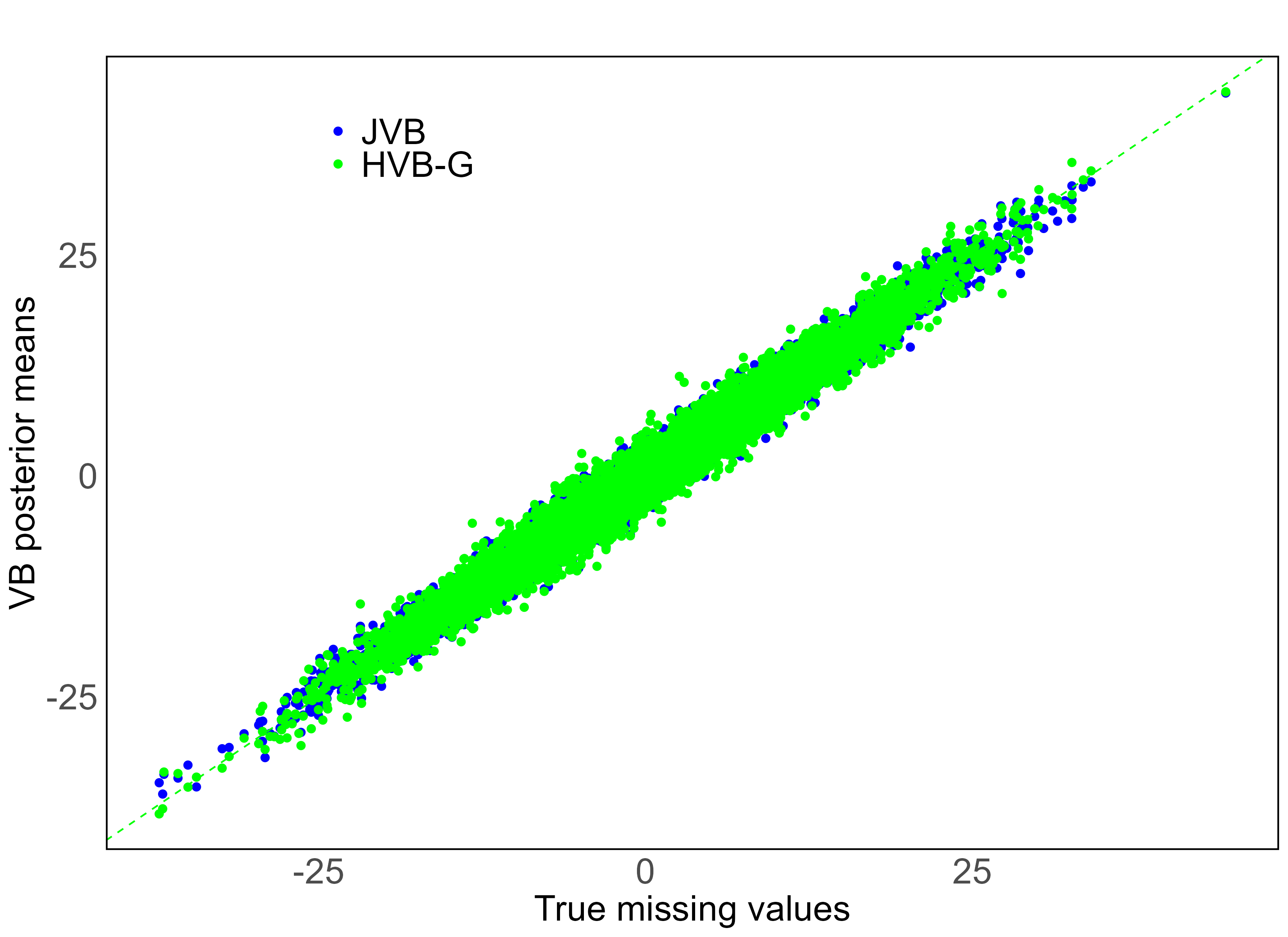
Algorithm 3 outlines the proposed Gibbs sampling steps. The full conditional distribution p(yuj|ϕ(t),yo,yu(j))=p(yujϕ(t),ysj)𝑝conditionalsubscriptysubscript𝑢𝑗superscriptbold-italic-ϕ𝑡subscripty𝑜superscriptsubscripty𝑢𝑗𝑝conditionalsubscriptysubscript𝑢𝑗superscriptbold-italic-ϕ𝑡subscriptysubscript𝑠𝑗p(\textbf{y}_{u_{j}}|\boldsymbol{\phi}^{(t)},\textbf{y}_{o},\textbf{y}_{u}^{(-j)})=p(\textbf{y}_{u_{j}}\mid\boldsymbol{\phi}^{(t)},\textbf{y}_{s_{j}}), follows a multivariate Gaussian distribution with the mean Xuj𝜷My,ujuj1My,ujsj(ysjXsj𝜷)subscriptXsubscript𝑢𝑗𝜷superscriptsubscriptM𝑦subscript𝑢𝑗subscript𝑢𝑗1subscriptM𝑦subscript𝑢𝑗subscript𝑠𝑗subscriptysubscript𝑠𝑗subscriptXsubscript𝑠𝑗𝜷\textbf{X}_{u_{j}}\boldsymbol{\beta}-\textbf{M}_{y,{u_{j}}{u_{j}}}^{-1}\textbf{M}_{y,{u_{j}}{s_{j}}}(\textbf{y}_{s_{j}}-\textbf{X}_{s_{j}}\boldsymbol{\beta}) and the covariance matrix σy2My,ujuj1subscriptsuperscript𝜎2ysuperscriptsubscriptM𝑦subscript𝑢𝑗subscript𝑢𝑗1\sigma^{2}_{\textbf{y}}\textbf{M}_{y,{u_{j}}{u_{j}}}^{-1}. The HVB algorithm implemented using the Gibbs steps presented in Algorithm 3, which we call HVB-G in subsequent sections, accelerates the generation of samples of missing values from their conditional distribution p(yuϕ,yo)𝑝conditionalsubscripty𝑢bold-italic-ϕsubscripty𝑜p(\textbf{y}_{u}\mid\boldsymbol{\phi},\textbf{y}_{o}) when n𝑛n and nusubscript𝑛𝑢n_{u} are large. We replace step 5 of the HVB algorithm given in Algorithm 2 by the proposed Gibbs steps when nusubscript𝑛𝑢n_{u} is more than 1,00010001,000 as directly sampling from p(yuϕ,yo)𝑝conditionalsubscripty𝑢bold-italic-ϕsubscripty𝑜p(\textbf{y}_{u}\mid\boldsymbol{\phi},\textbf{y}_{o}) requires inverting a 1000×1000100010001000\times 1000 covariance matrix. In the Gibbs sampling steps, we must specify the block size (ksuperscript𝑘k^{*}) and the number of Gibbs iterations (N1subscript𝑁1N_{1}). After some experimentation, we set N1=5subscript𝑁15N_{1}=5 with a block size of k=500superscript𝑘500k^{*}=500, as these values consistently produce accurate inference results within a reasonable computational time.

Algorithm 3 Gibbs steps within the tthsuperscript𝑡𝑡t^{th} iteration of the HVB algorithm under MAR when n𝑛n and nusubscript𝑛𝑢n_{u} are large
1:  Initialise missing values yu,0=(yu1,0,,yuk,0)p(yuϕ(t),yo)subscripty𝑢0superscriptsuperscriptsubscriptysubscript𝑢10topsuperscriptsubscriptysubscript𝑢𝑘0toptopsimilar-to𝑝conditionalsubscripty𝑢superscriptbold-italic-ϕ𝑡subscripty𝑜\textbf{y}_{u,0}=(\textbf{y}_{u_{1},0}^{\top},\dots,\textbf{y}_{u_{k},0}^{\top})^{\top}~{}\sim p(\textbf{y}_{u}\mid\boldsymbol{\phi}^{(t)},\textbf{y}_{o})
2:  for i=1, …, N1subscript𝑁1N_{1} do
3:     for j=1, …, k do
4:        Sample yuj,isubscriptysubscript𝑢𝑗𝑖\textbf{y}_{u_{j},i} from the conditional distribution p(yuj,iϕ(t),yo,yu,i1(j))𝑝conditionalsubscriptysubscript𝑢𝑗𝑖superscriptbold-italic-ϕ𝑡subscripty𝑜superscriptsubscripty𝑢𝑖1𝑗p(\textbf{y}_{u_{j},i}\mid\boldsymbol{\phi}^{(t)},\textbf{y}_{o},\textbf{y}_{u,i-1}^{(-j)}), where yu,i1(j)=(yu1,i,yu2,i,,yuj1,i,yuj+1,i1,,,yuk,i1)\textbf{y}_{u,i-1}^{(-j)}=(\textbf{y}^{\top}_{u_{1},i},\textbf{y}^{\top}_{u_{2},i},\ldots,\textbf{y}^{\top}_{u_{j-1},i},\textbf{y}^{\top}_{u_{j+1},i-1},\ldots,,\textbf{y}^{\top}_{u_{k},i-1})^{\top}.
5:     end for
6:     yu,i=(yu1,i,,yuk,i)subscripty𝑢𝑖superscriptsuperscriptsubscriptysubscript𝑢1𝑖topsuperscriptsubscriptysubscript𝑢𝑘𝑖toptop\textbf{y}_{u,i}=(\textbf{y}_{u_{1},i}^{\top},\ldots,\textbf{y}_{u_{k},i}^{\top})^{\top}
7:  end for
8:  Output yu(t)=yu,N1superscriptsubscripty𝑢𝑡subscripty𝑢subscript𝑁1\textbf{y}_{u}^{(t)}=\textbf{y}_{u,N_{1}}

3.5 HVB under MNAR

Under MNAR, direct sampling from the conditional distribution p(𝐲u𝜽(t),𝐎)=p(𝐲uϕ(t),𝝍(t),𝐲o,𝐦)𝑝conditionalsubscript𝐲𝑢superscript𝜽𝑡𝐎𝑝conditionalsubscript𝐲𝑢superscriptbold-italic-ϕ𝑡superscript𝝍𝑡subscript𝐲𝑜𝐦p(\mathbf{y}_{u}\mid\boldsymbol{\theta}^{(t)},\mathbf{O})=p(\mathbf{y}_{u}\mid\boldsymbol{\phi}^{(t)},\boldsymbol{\psi}^{(t)},\mathbf{y}_{o},\mathbf{m}) is not feasible, as the conditional posterior distribution is not available in closed form. To sample from p(𝐲uϕ(t),𝝍(t),𝐲o,𝐦)𝑝conditionalsubscript𝐲𝑢superscriptbold-italic-ϕ𝑡superscript𝝍𝑡subscript𝐲𝑜𝐦p(\mathbf{y}_{u}\mid\boldsymbol{\phi}^{(t)},\boldsymbol{\psi}^{(t)},\mathbf{y}_{o},\mathbf{m}), we employ the MCMC steps presented in Algorithm 4, which employs p(yuϕ(t),yo)𝑝conditionalsubscripty𝑢superscriptbold-italic-ϕ𝑡subscripty𝑜p(\textbf{y}_{u}\mid\boldsymbol{\phi}^{(t)},\textbf{y}_{o}) as the proposal.

Algorithm 4 MCMC steps within the tthsuperscript𝑡𝑡t^{th} iteration of the HVB algorithm under MNAR
1:  Initialize missing values yu,0p(yuϕ(t),yo)similar-tosubscripty𝑢0𝑝conditionalsubscripty𝑢superscriptbold-italic-ϕ𝑡subscripty𝑜\textbf{y}_{u,0}~{}\sim p(\textbf{y}_{u}\mid\boldsymbol{\phi}^{(t)},\textbf{y}_{o})
2:  for i=1, …, N1subscript𝑁1N_{1} do
3:     Sample yusuperscriptsubscripty𝑢\textbf{y}_{u}^{*} from the proposal distribution p(yuϕ(t),yo)𝑝conditionalsuperscriptsubscripty𝑢superscriptbold-italic-ϕ𝑡subscripty𝑜p(\textbf{y}_{u}^{*}\mid\boldsymbol{\phi}^{(t)},\textbf{y}_{o}), which follows a multivariate Gaussian with the mean vector given by Xu𝜷My,uu1My,uo(yoXo𝜷)subscriptX𝑢𝜷superscriptsubscriptM𝑦𝑢𝑢1subscriptM𝑦𝑢𝑜subscripty𝑜subscriptX𝑜𝜷\textbf{X}_{u}\boldsymbol{\beta}-\textbf{M}_{y,uu}^{-1}\textbf{M}_{y,uo}(\textbf{y}_{o}-\textbf{X}_{o}\boldsymbol{\beta}) and the covariance matrix given by σy2My,uu1subscriptsuperscript𝜎2ysuperscriptsubscriptM𝑦𝑢𝑢1\sigma^{2}_{\textbf{y}}\textbf{M}_{y,uu}^{-1}.
4:     Sample u𝑢u from uniform distribution, u𝒰(0,1)similar-to𝑢𝒰01u~{}\sim\mathcal{U}(0,1)
5:     Calculate a=min(1,p(my,𝝍(t))p(myi1,𝝍(t)))𝑎min1𝑝conditionalmsuperscriptysuperscript𝝍𝑡𝑝conditionalmsubscripty𝑖1superscript𝝍𝑡a=\text{min}\left(1,\frac{p(\textbf{m}\mid\textbf{y}^{*},\boldsymbol{\psi}^{(t)})}{p(\textbf{m}\mid\textbf{y}_{{i-1}},\boldsymbol{\psi}^{(t)})}\right), where y=(yo,yu)superscriptysuperscriptsubscripty𝑜topsuperscriptsuperscriptsubscripty𝑢top\textbf{y}^{*}=(\textbf{y}_{o}^{\top},{\textbf{y}_{u}^{*}}^{\top}) and yi1=(yo,yu,i1)subscripty𝑖1subscriptsuperscriptytop𝑜subscriptsuperscriptytop𝑢𝑖1\textbf{y}_{i-1}=(\textbf{y}^{\top}_{o},{\textbf{y}^{\top}_{u,{i-1}}})
6:     if a>u𝑎𝑢a>u then
7:        yu,i=yusubscripty𝑢𝑖superscriptsubscripty𝑢\textbf{y}_{u,i}=\textbf{y}_{u}^{*}
8:     else
9:        yu,i=yu,i1subscripty𝑢𝑖subscripty𝑢𝑖1\textbf{y}_{u,i}=\textbf{y}_{u,i-1}
10:     end if
11:  end for
12:  Output yu(t)=yu,N1subscriptsuperscripty𝑡𝑢subscripty𝑢subscript𝑁1\textbf{y}^{(t)}_{u}=\textbf{y}_{u,N_{1}}

The MCMC steps in Algorithm 4 generates samples from the conditional distribution p(yuϕ(t),𝝍(t),yo,m)𝑝conditionalsubscripty𝑢superscriptbold-italic-ϕ𝑡superscript𝝍𝑡subscripty𝑜mp(\textbf{y}_{u}\mid\boldsymbol{\phi}^{(t)},\boldsymbol{\psi}^{(t)},\textbf{y}_{o},\textbf{m}). However, as n𝑛n and nusubscript𝑛𝑢n_{u} increase, the HVB algorithm implemented using these MCMC steps does not estimate the parameters accurately because of the low acceptance percentage. After some experimentation, we found that achieving an acceptance percentage between 20%percent2020\% and 30%percent3030\% is necessary to balance between accurate posterior inference and computational cost. To improve the acceptance percentage, we partition yusubscripty𝑢\textbf{y}_{u} into k𝑘k blocks as discussed in Section 3.4, and update one block at a time using proposals from p(yujϕ(t),yo,yu(j))𝑝conditionalsubscriptysubscript𝑢𝑗superscriptbold-italic-ϕ𝑡subscripty𝑜superscriptsubscripty𝑢𝑗p(\textbf{y}_{u_{j}}\mid\boldsymbol{\phi}^{(t)},\textbf{y}_{o},\textbf{y}_{u}^{(-j)}). Algorithm 5 outlines the MCMC steps for sampling the missing values one block at a time.

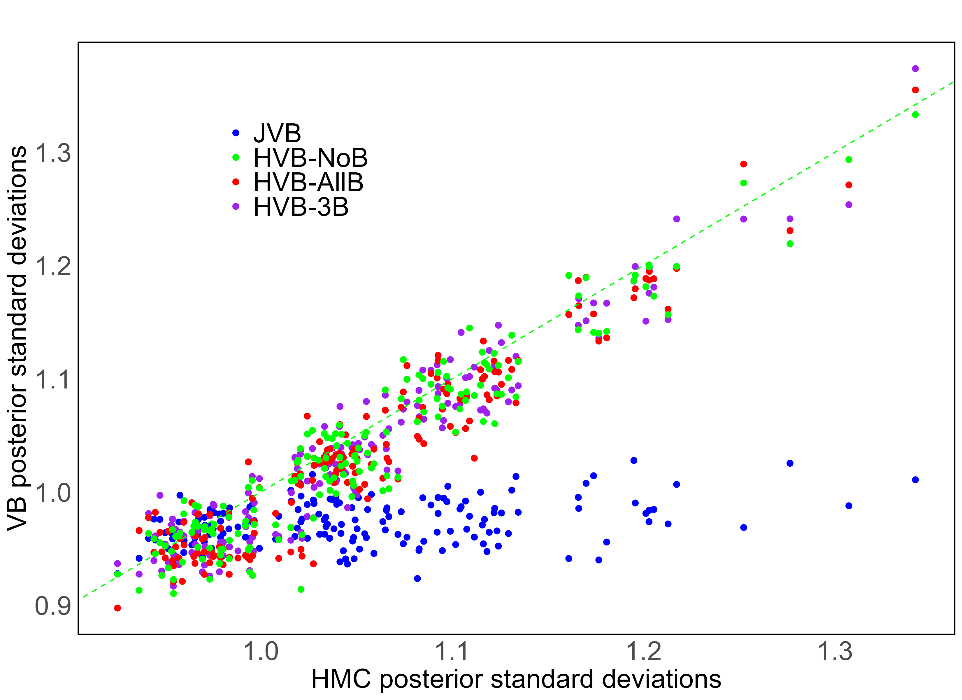
Updating all k𝑘k blocks for each of the N1subscript𝑁1N_{1} MCMC iterations is computationally expensive, as for each block, the mean vector and covariance matrix of the conditional posterior distribution of p(yujϕ,ysj)𝑝conditionalsubscriptysubscript𝑢𝑗bold-italic-ϕsubscriptysubscript𝑠𝑗p(\textbf{y}_{u_{j}}\mid\boldsymbol{\phi},\textbf{y}_{s_{j}}) must be calculated. This computational bottleneck can be overcome by updating only a randomly selected set of blocks at each iteration, so the computation of the conditional distribution is limited to the number of updated blocks, not the number of total blocks, k𝑘k. We suggest that updating randomly selected 333 blocks in each MCMC iteration is sufficient to obtain reliable inference with a smaller computational cost; see simulation results in Section 4.2 for further details. The MCMC scheme for updating a randomly selected number of ksuperscript𝑘k^{\prime} blocks can be obtained by modifying the MCMC scheme in Algorithm 5.

Algorithm 5 MCMC steps within the tthsuperscript𝑡𝑡t^{th} iteration of the HVB algorithm under MNAR. The missing values are updated one block at a time
1:  Initialize missing values yu,0=(yu1,0,,yuk,0)p(yuϕ(t),yo)subscripty𝑢0superscriptsubscriptsuperscriptytopsubscript𝑢10subscriptsuperscriptytopsubscript𝑢𝑘0topsimilar-to𝑝conditionalsubscripty𝑢superscriptbold-italic-ϕ𝑡subscripty𝑜\textbf{y}_{u,0}=(\textbf{y}^{\top}_{u_{1},0},\dots,\textbf{y}^{\top}_{u_{k},0})^{\top}~{}\sim p(\textbf{y}_{u}\mid\boldsymbol{\phi}^{(t)},\textbf{y}_{o})
2:  for i=1, …, N1subscript𝑁1N_{1} do
3:     for j=1, …, k𝑘k do
4:        Sample yujsuperscriptsubscriptysubscript𝑢𝑗\textbf{y}_{u_{j}}^{*} from the proposal distribution p(yujϕ(t),yo,yu,i1(j))𝑝conditionalsuperscriptsubscriptysubscript𝑢𝑗superscriptbold-italic-ϕ𝑡subscripty𝑜superscriptsubscripty𝑢𝑖1𝑗p(\textbf{y}_{u_{j}}^{*}\mid\boldsymbol{\phi}^{(t)},\textbf{y}_{o},\textbf{y}_{u,{i-1}}^{(-j)}), where yu,i1(j)=(yu1,i,yu2,i,,yuj1,i,yuj+1,i1,,,yuk,i1)\textbf{y}_{u,i-1}^{(-j)}=(\textbf{y}^{\top}_{u_{1},i},\textbf{y}^{\top}_{u_{2},i},\ldots,\textbf{y}^{\top}_{u_{j-1},i},\textbf{y}^{\top}_{u_{j+1},i-1},\ldots,,\textbf{y}^{\top}_{u_{k},i-1})^{\top}.
5:        Sample u𝑢u from uniform distribution, u𝒰(0,1)similar-to𝑢𝒰01u~{}\sim\mathcal{U}(0,1)
6:        Calculate a=min(1,p(my,𝝍(t))p(myi1,𝝍(t)))𝑎min1𝑝conditionalmsuperscriptysuperscript𝝍𝑡𝑝conditionalmsubscripty𝑖1superscript𝝍𝑡a=\text{min}\left(1,\frac{p(\textbf{m}\mid\textbf{y}^{*},\boldsymbol{\psi}^{(t)})}{p(\textbf{m}\mid\textbf{y}_{i-1},\boldsymbol{\psi}^{(t)})}\right), where y=(yo,yu(j),yuj)superscriptysuperscriptsuperscriptsubscripty𝑜topsuperscriptsuperscriptsubscripty𝑢𝑗topsuperscriptsuperscriptsubscriptysubscript𝑢𝑗toptop\textbf{y}^{*}=(\textbf{y}_{o}^{\top},{\textbf{y}_{u}^{(-j)}}^{\top},{\textbf{y}_{u_{j}}^{*}}^{\top})^{\top} and yi1=(yo,yu(j),yuj,i1)subscripty𝑖1superscriptsuperscriptsubscripty𝑜topsuperscriptsuperscriptsubscripty𝑢𝑗topsuperscriptsubscriptysubscript𝑢𝑗𝑖1toptop\textbf{y}_{i-1}=(\textbf{y}_{o}^{\top},{\textbf{y}_{u}^{(-j)}}^{\top},{\textbf{y}_{u_{j},{i-1}}}^{\top})^{\top}
7:        if a>u𝑎𝑢a>u then
8:           yuj,i=yujsubscriptysubscript𝑢𝑗𝑖superscriptsubscriptysubscript𝑢𝑗\textbf{y}_{u_{j},i}=\textbf{y}_{u_{j}}^{*}
9:        else
10:           yuj,i=yuj,i1subscriptysubscript𝑢𝑗𝑖subscriptysubscript𝑢𝑗𝑖1\textbf{y}_{u_{j},i}=\textbf{y}_{{u_{j},i-1}}
11:        end if
12:     end for
13:     yu,i=(yu1,i,,yuk,i)subscripty𝑢𝑖superscriptsuperscriptsubscriptysubscript𝑢1𝑖topsuperscriptsubscriptysubscript𝑢𝑘𝑖toptop\textbf{y}_{u,i}=(\textbf{y}_{u_{1},i}^{\top},\ldots,\textbf{y}_{u_{k},i}^{\top})^{\top}
14:  end for
15:  Output yu(t)=yu,N1subscriptsuperscripty𝑡𝑢subscripty𝑢subscript𝑁1\textbf{y}^{(t)}_{u}=\textbf{y}_{u,N_{1}}

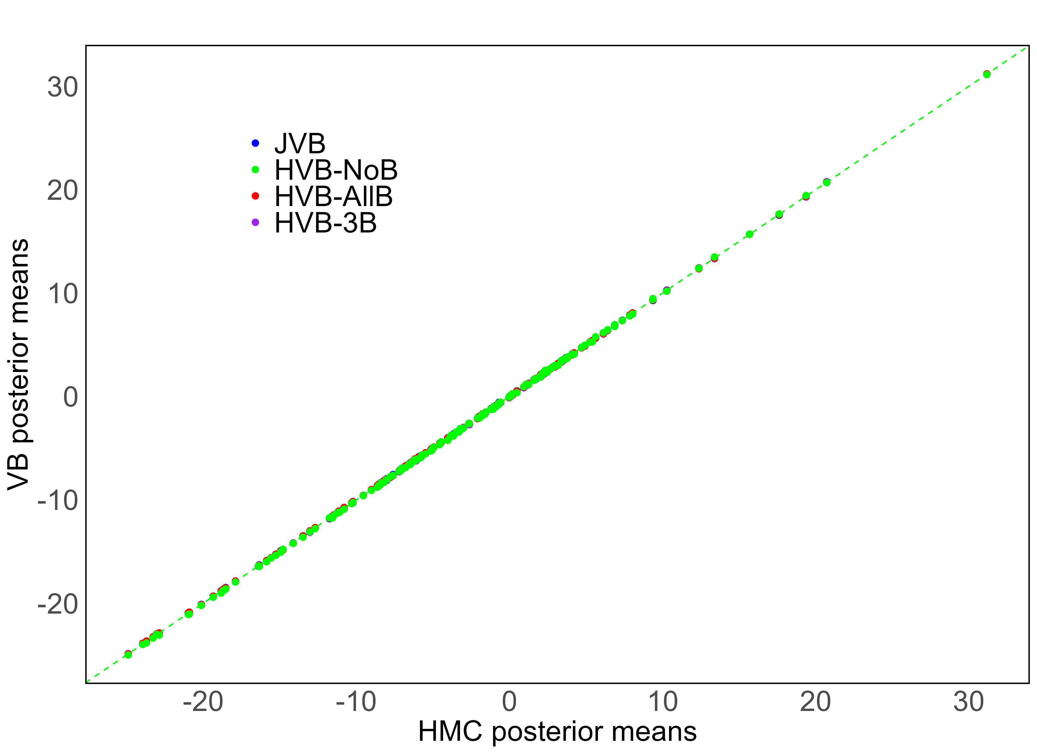
For the remaining sections, the HVB algorithm implemented via the MCMC scheme in Algorithm 4 without blocking yusubscripty𝑢\textbf{y}_{u} is called the HVB-No Block abbreviated as HVB-NoB. The HVB algorithm implemented through the MCMC scheme in Algorithm 5 is called HVB-All Block abbreviated as HVB-AllB, and the HVB using the MCMC scheme that updates only randomly selected three blocks is referred to as HVB-3B. The criteria for setting tuning parameters of the proposed MCMC schemes, such as the number of MCMC steps N1subscript𝑁1N_{1} and block size ksuperscript𝑘k^{*}, are discussed in Section 4.2.

4 Simulation result

This section investigates the performance of the VB methods to estimate the SEM under MAR and MNAR mechanisms. We compare the posterior density estimates from the VB methods to those obtained from the Hamiltonian Monte Carlo method (HMC). All examples are implemented using the R programming language. The HMC is implemented using the RStan interface (Stan Development Team,, 2023). We use the HMC method from Hoffman et al., (2014), known as the No U-Turn Sampler (NUTS). For details on the generic HMC algorithm, see Section  S3 of the online supplement.

In all simulation studies, we simulate n𝑛n observations from a standard SEM according to Equation (1) with 101010 covariates. Each covariate for every observation is drawn from a standard normal distribution N(0,1)𝑁01N(0,1). The weight matrices are constructed based on a regular grid of size n×n𝑛𝑛\sqrt{n}\times\sqrt{n}, where neighbours are defined using the Rook neighbourhood method (refer to Wijayawardhana et al., (2024) for details on constructing the weight matrix based on the Rook neighbourhood). We generate the true values of the 111111 fixed effects (𝜷𝜷\boldsymbol{\beta}’s) randomly from discrete uniform random numbers between 111 and 555. We set σ𝒚2=1subscriptsuperscript𝜎2𝒚1\sigma^{2}_{\boldsymbol{y}}=1 and ρ=0.8𝜌0.8\rho=0.8. The subsequent steps in the simulation process vary depending on the missing value mechanisms.

For the MAR mechanism, after simulating n𝑛n observations from a standard SEM, we randomly select nosubscript𝑛𝑜n_{o} units to form the observed data set. In the MNAR mechanism, we generate missing responses using the logistic regression model regressed on a randomly chosen covariate from the 10 covariates and the response variable of SEM (y) as covariates, which is given by

p(my,X,𝝍)=i=1nexi𝝍x+yiψy1+exi𝝍x+yiψy,𝑝conditionalmysuperscriptX𝝍superscriptsubscriptproduct𝑖1𝑛superscript𝑒subscriptsuperscriptx𝑖subscript𝝍xsubscript𝑦𝑖subscript𝜓𝑦1superscript𝑒subscriptsuperscriptx𝑖subscript𝝍xsubscript𝑦𝑖subscript𝜓𝑦p(\textbf{m}\mid\textbf{y},\textbf{X}^{*},\boldsymbol{\psi})=\prod_{i=1}^{n}\frac{e^{\textbf{x}^{*}_{i}\boldsymbol{\psi}_{\textbf{x}}+{y}_{i}\psi_{y}}}{1+e^{\textbf{x}^{*}_{i}\boldsymbol{\psi}_{\textbf{x}}+{y}_{i}\psi_{y}}}, (22)

where the design matrix XsuperscriptX\textbf{X}^{*} contains a column of ones and the selected covariate, and 𝕩isuperscriptsubscript𝕩𝑖\mathbb{x}_{i}^{*} denotes the ithsuperscript𝑖𝑡i^{th} row vector of 𝕏superscript𝕏\mathbb{X}^{*}. The vector 𝝍x=(ψ0,ψx)subscript𝝍xsubscript𝜓0subscript𝜓superscriptx\boldsymbol{\psi}_{\textbf{x}}=(\psi_{0},\psi_{\textbf{x}^{*}}) contains the coefficient of the intercept (ψ0subscript𝜓0\psi_{0}), and the coefficient of the selected covariate (ψxsubscript𝜓superscriptx\psi_{\textbf{x}^{*}}). The coefficient corresponding to y is ψysubscript𝜓y\psi_{\textbf{y}}.

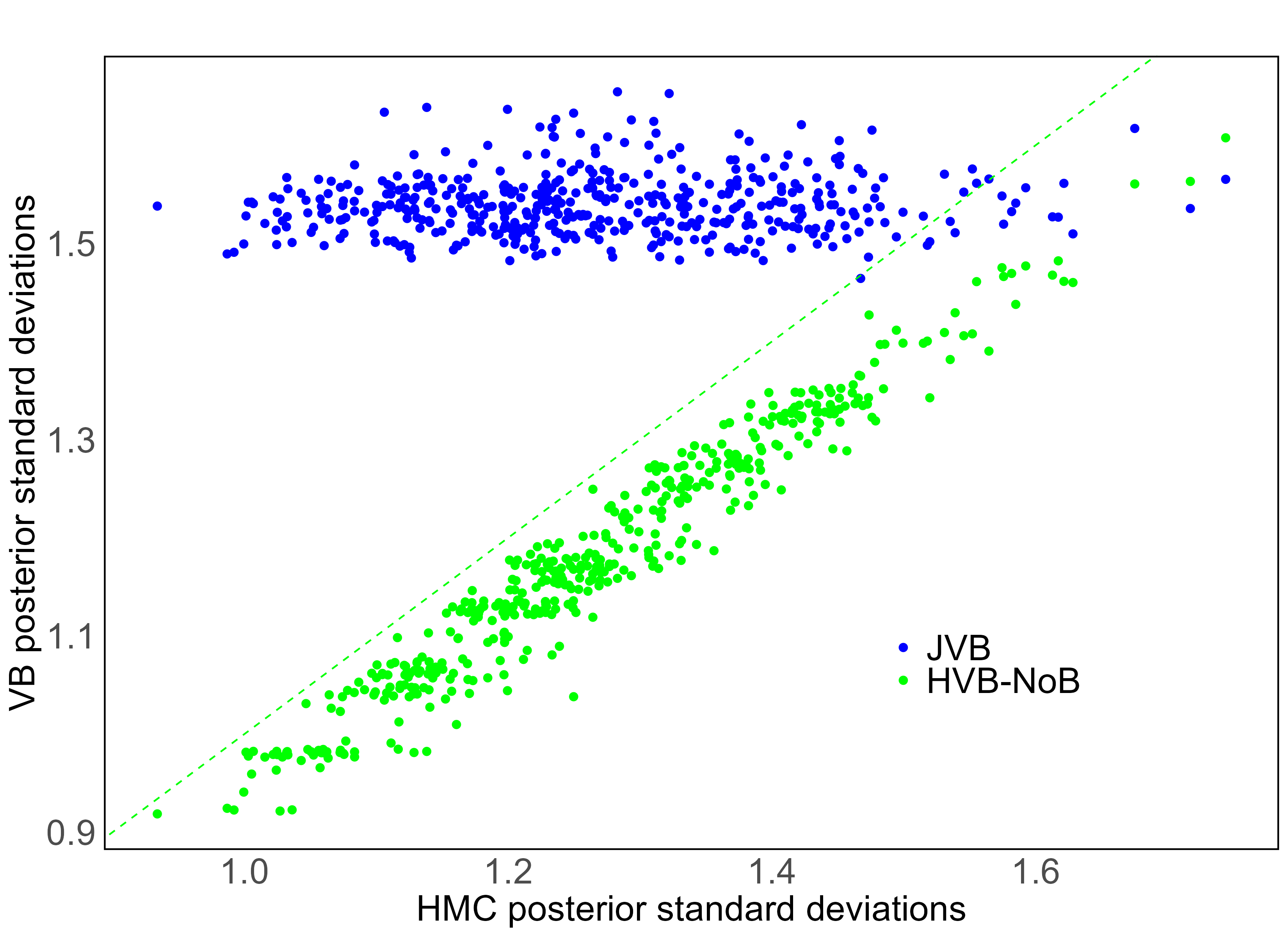
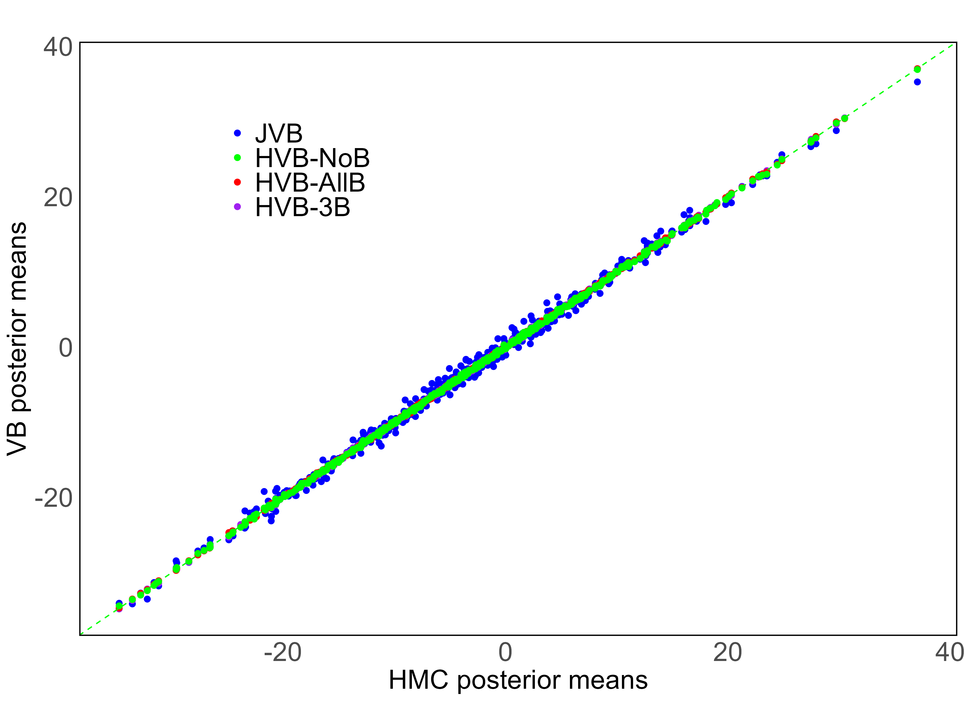
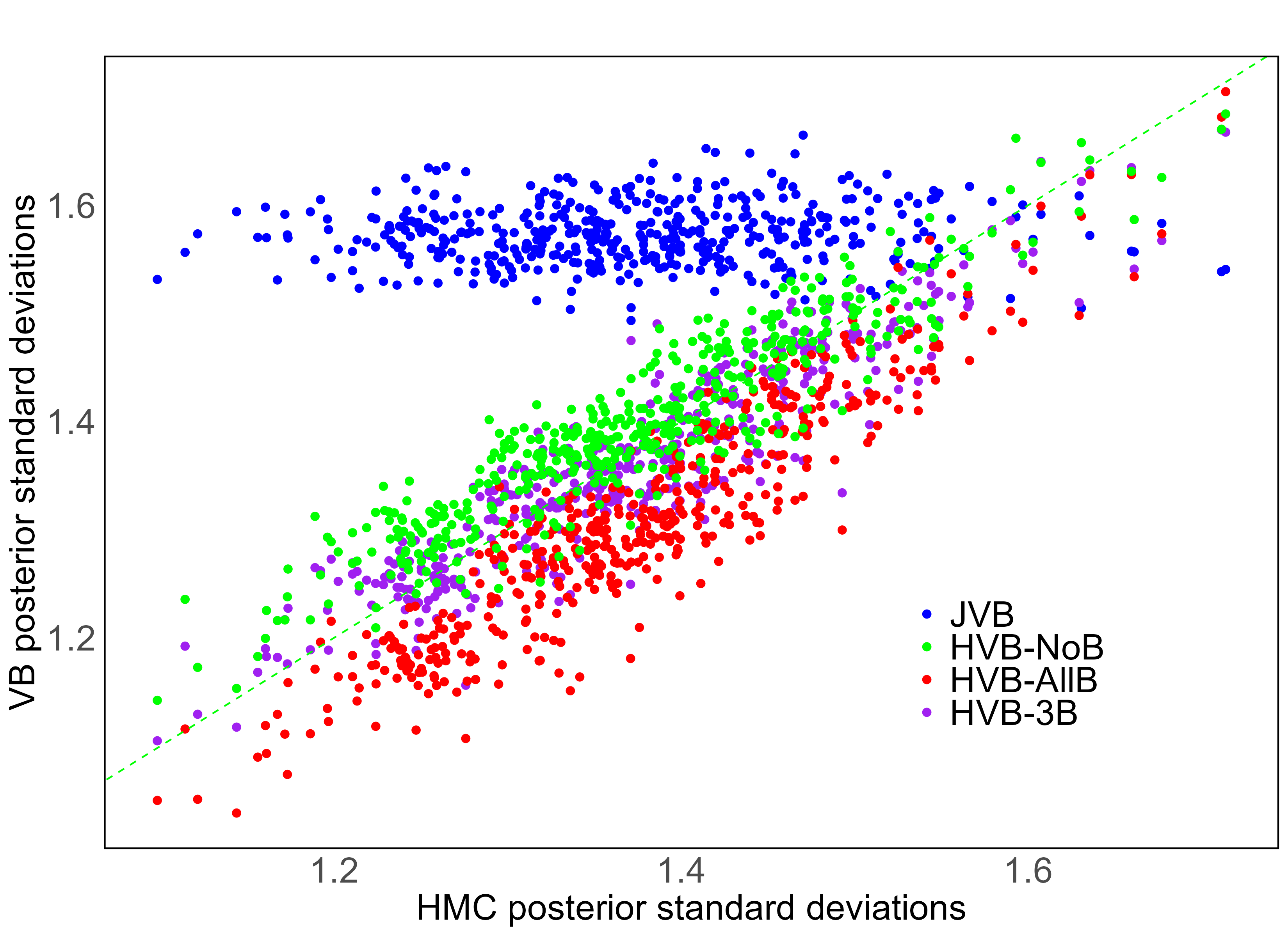
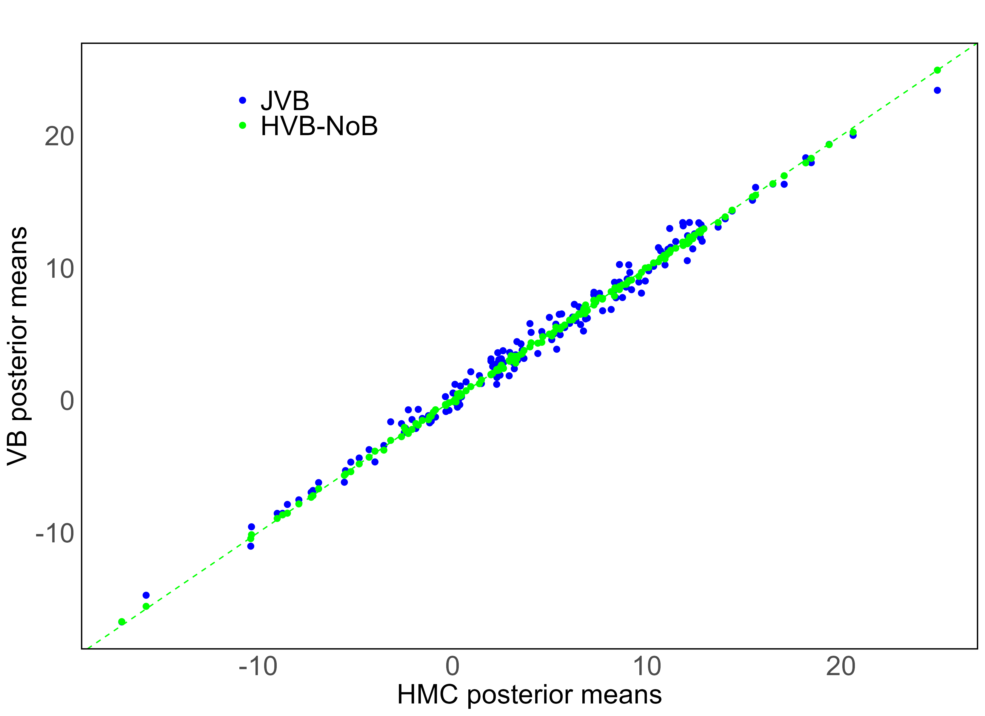
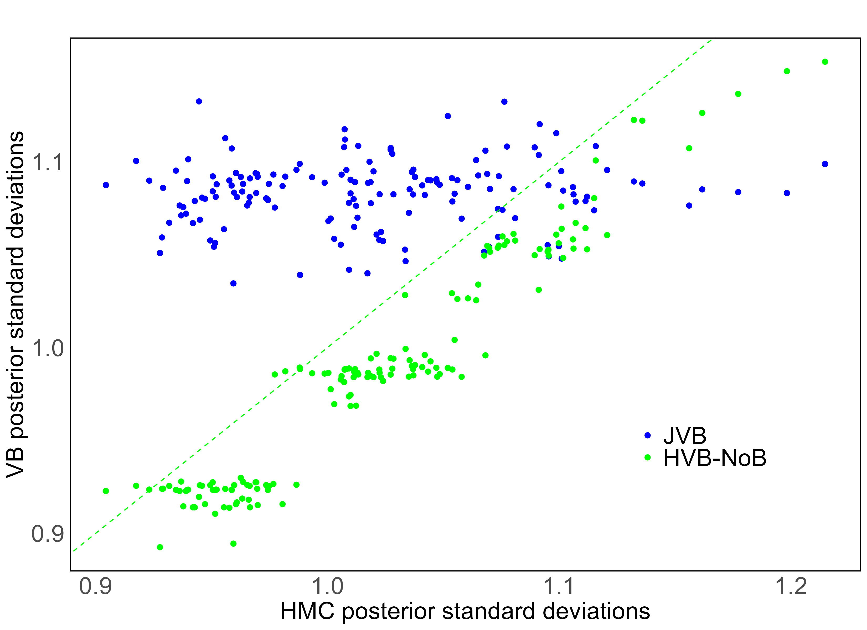
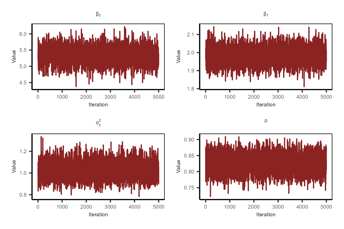
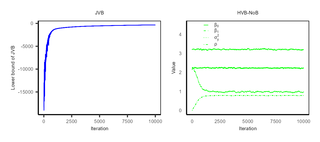
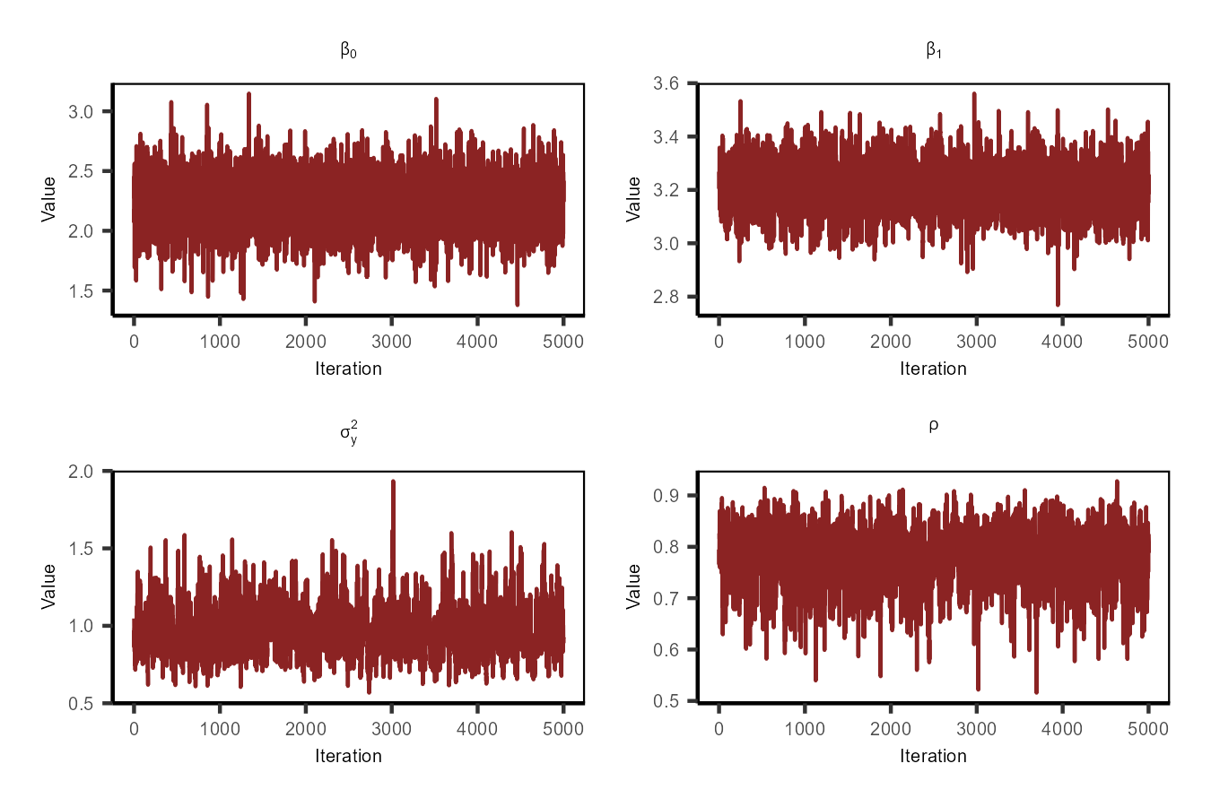
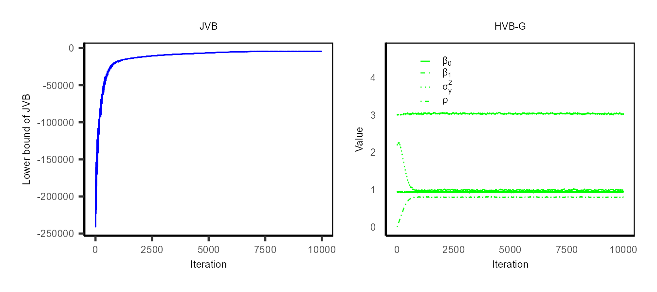
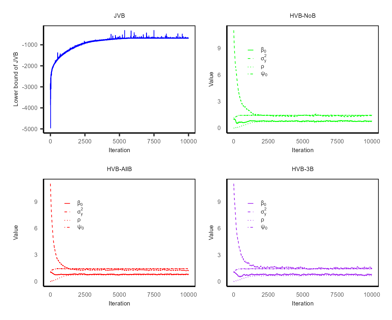
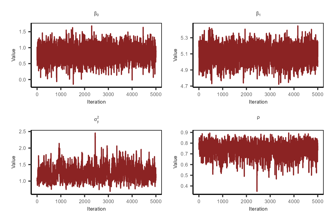
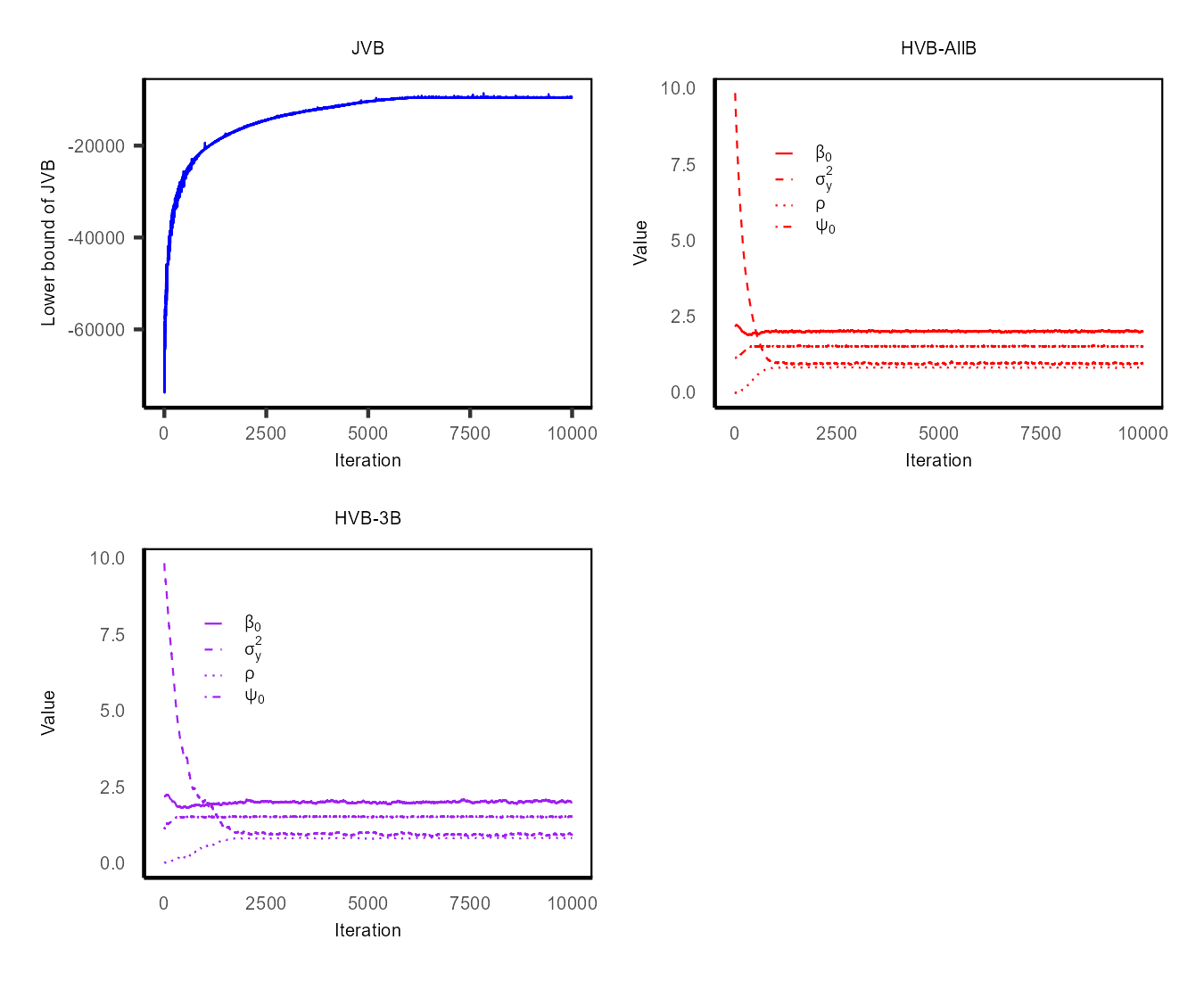
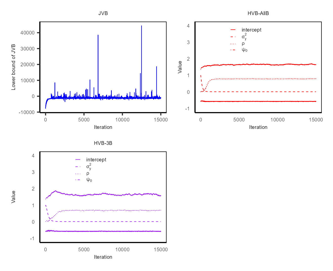
All VB and HMC algorithms in this work utilise the same prior distributions, p(𝜽)𝑝𝜽p(\boldsymbol{\theta}), for the parameters (under MAR p(𝜽)=p(ϕ)𝑝𝜽𝑝bold-italic-ϕp(\boldsymbol{\theta})=p(\boldsymbol{\phi}), and under MNAR p(𝜽)=p(ϕ,𝝍)=p(ϕ)p(𝝍)𝑝𝜽𝑝bold-italic-ϕ𝝍𝑝bold-italic-ϕ𝑝𝝍p(\boldsymbol{\theta})=p(\boldsymbol{\phi},\boldsymbol{\psi})=p(\boldsymbol{\phi})p(\boldsymbol{\boldsymbol{\psi}})). The priors for the parameters are given in Section S2 of the online supplement. When implementing VB algorithms, the initial values are set as follows: Under MAR, the ordinary least squares (OLS) estimates are used for the initial values for the fixed effect parameters (𝜷𝜷\boldsymbol{\beta}’s) and the error variance (σy2subscriptsuperscript𝜎2y\sigma^{2}_{\textbf{y}}). Additionally, we assign a value of 0.01 to ρ𝜌\rho, reflecting a very weak spatial dependence. Under MNAR, we have additional three parameters ψ0,ψxsubscript𝜓0subscript𝜓superscriptx\psi_{0},\psi_{\textbf{x}^{*}} and ψysubscript𝜓y\psi_{\textbf{y}}. For all these coefficients, we set the starting value to 0.010.010.01. The initial values for the missing data under MAR and MNAR are simulated from the conditional distribution p(yuϕ(0),yo)𝑝conditionalsubscripty𝑢superscriptbold-italic-ϕ0subscripty𝑜p(\textbf{y}_{u}\mid\boldsymbol{\phi}^{(0)},\textbf{y}_{o}), where ϕ(0)superscriptbold-italic-ϕ0\boldsymbol{\phi}^{(0)} is the vector containing the initial parameter values. We use p=4𝑝4p=4 factors for HVB and JVB for the simulation study. The results do not improve when we increase the number of factors. We run the VB and HMC methods for 10,0001000010,000 iterations for all simulation studies. Section S7 of the online supplement presents convergence plots for the VB algorithms and trace plots of posterior samples from HMC.

In Section 4.1, we examine the accuracy and computational cost of proposed VB methods for estimating SEM under the MAR mechanism. Section 4.2 presents the simulation results for estimating SEM under the MNAR mechanism.

4.1 Simulation study under MAR

This section discusses the simulation results for estimating SEM under the MAR mechanism. We investigate the accuracy of the proposed VB methods using two sample sizes: n=625𝑛625n=625 and n=10,000𝑛10000n=10,000. For n=625𝑛625n=625, we consider scenarios with 25%percent2525\% and 75%percent7575\% missing data. For n=10,000𝑛10000n=10,000, we only consider the scenario with 75%percent7575\% missing data. This section discusses the results for the 75%percent7575\% missing data scenario for n=625𝑛625n=625 and n=10,000𝑛10000n=10,000. The results for n=625𝑛625n=625 with 25% missing data are provided in Section S4.1 of the online supplement.

Figure 1 presents the posterior densities of SEM parameters estimated using the HMC, JVB, and HVB methods for the simulated dataset with n=625𝑛625n=625 and 75%percent7575\% missing values (nu=468subscript𝑛𝑢468n_{u}=468). Since nusubscript𝑛𝑢n_{u} is small (<1,000absent1000<1,000), we use the standard HVB without the Gibbs steps, the HVB-NoB method, given in Algorithm 2. For the fixed effects parameters (𝜷𝜷\boldsymbol{\beta}’s), the posterior densities from the JVB and HVB-NoB are nearly identical to those from HMC, with HVB-NoB being the closest to HMC. However, the posterior densities of σy2subscriptsuperscript𝜎2y\sigma^{2}_{\textbf{y}} and ρ𝜌\rho from the JVB method exhibit significant deviations from those obtained by HMC, whereas the posterior densities from the HVB align well with those of HMC.
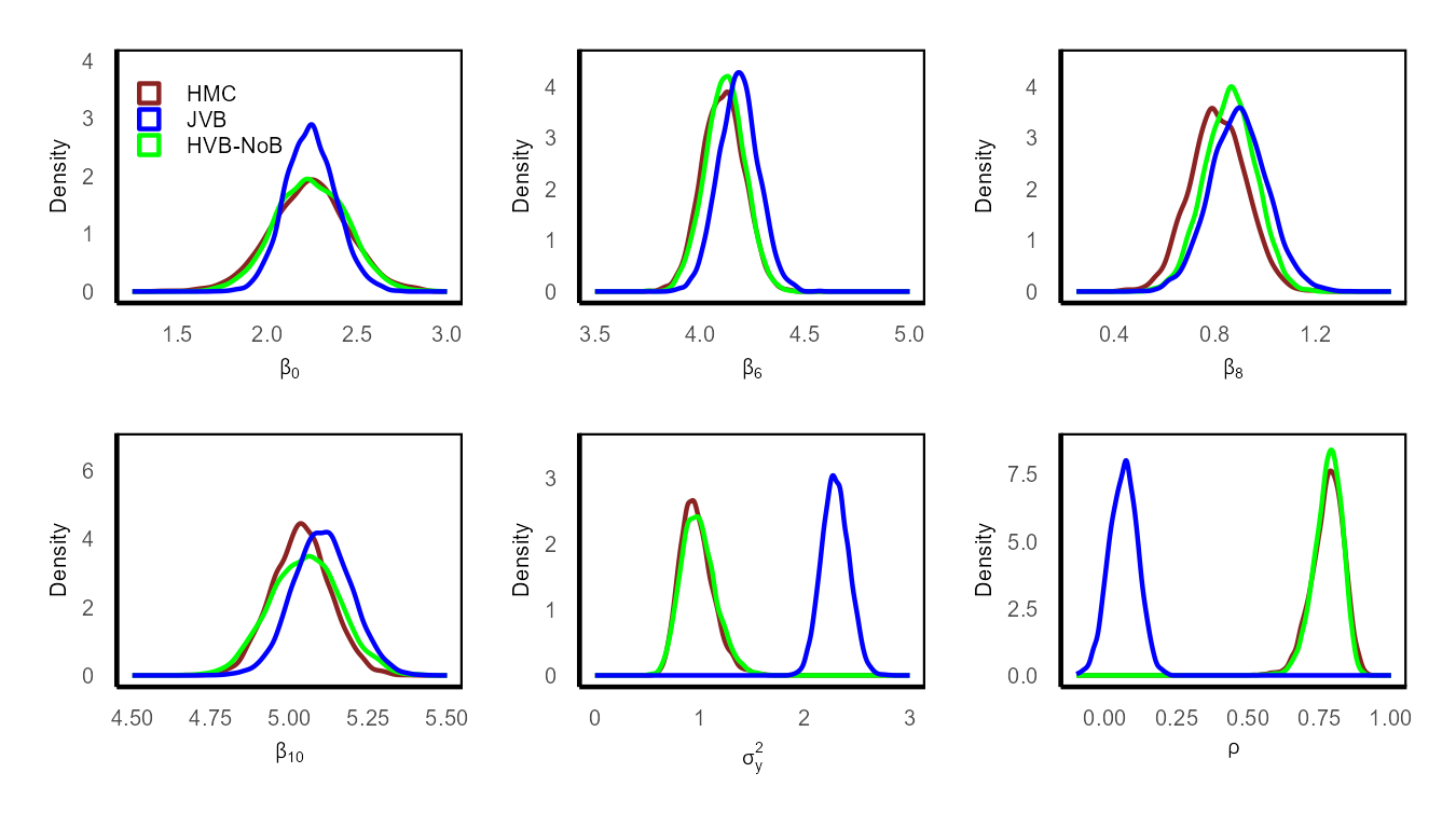
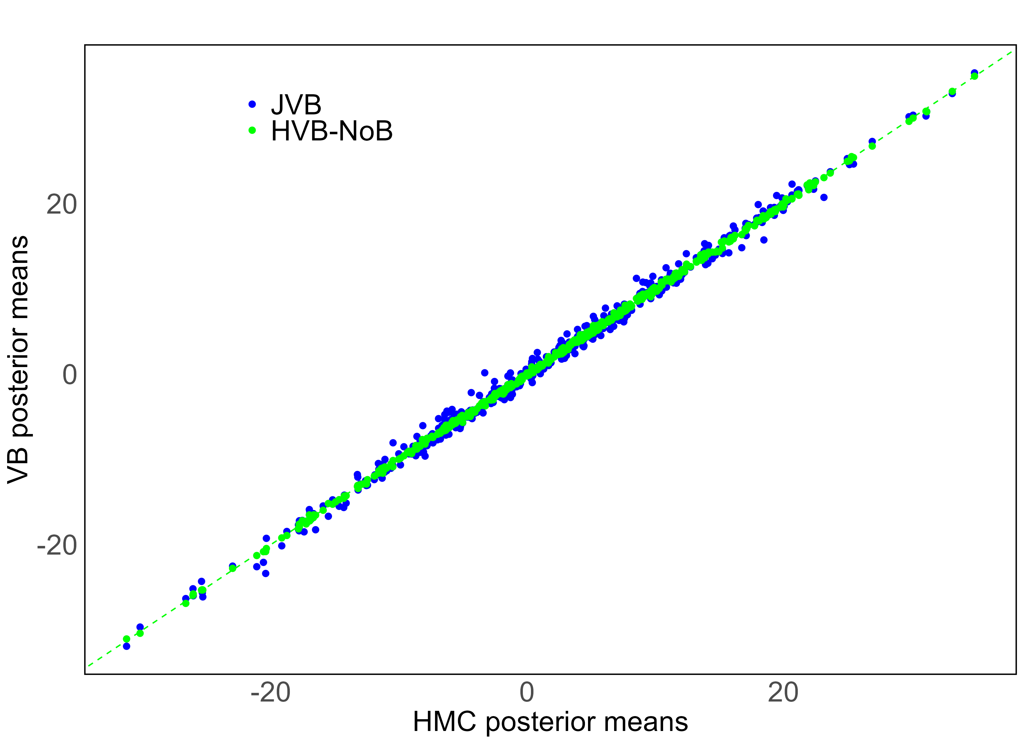
Refer to caption
Figure 1: Posterior densities of SEM parameters under MAR for the simulated dataset with n=625𝑛625n=625 and nu=468subscript𝑛𝑢468n_{u}=468 (75%percent7575\% missing values) estimated using the HMC, JVB and HVB-NoB methods
Refer to caption
(a) Posterior means
Refer to caption
(b) Posterior standard deviations
Figure 2: Comparison of the posterior means and standard deviations of the missing values obtained from JVB and HVB-NoB with those of HMC under MAR for the simulated data with n=625𝑛625n=625 and nu=468subscript𝑛𝑢468n_{u}=468 (75%percent7575\% missing values)

Figure 2 shows the comparison between the posterior means and standard deviations of the missing values obtained from the JVB, HVB-NoB, and HMC methods for the simulated dataset with n=625𝑛625n=625 and nu=468subscript𝑛𝑢468n_{u}=468. The posterior means obtained from the JVB and HVB-NoB methods are very close to those obtained from the HMC method, as shown in Figure 2(a). However, the posterior standard deviations estimated from the JVB method are significantly different from those obtained using the HMC method, as shown in Figure 2(b). On the other hand, the posterior standard deviations estimated from the HVB-NoB method are very close to those of the HMC method.

To investigate the accuracy of the VB methods with relatively large n𝑛n and missing values nusubscript𝑛𝑢n_{u}, we simulated a dataset with n=10,000𝑛10000n=10,000 and nu=7,500subscript𝑛𝑢7500n_{u}=7,500 (i.e. missing percentage is 75%percent7575\%) under MAR. As indicated in Table S2 in Section S4.1 of the online supplement, the average time taken per HMC iteration is notably high for high values of n𝑛n and nusubscript𝑛𝑢n_{u}, making practical implementation of HMC infeasible. Further, when the number of units (nusubscript𝑛𝑢n_{u}) is large (exceeding 1,000), utilising the standard HVB without the Gibbs steps becomes computationally intensive. We employ the HVB-G method with N1=5subscript𝑁15N_{1}=5 and k=500superscript𝑘500k^{*}=500 and the JVB method. Table 3 compares the posterior means of the parameters obtained using the two VB methods with their true parameter values. Similar to the simulation results obtained from the simulated dataset with n=625𝑛625n=625, the HVB-G method accurately estimates the posterior means of SEM parameters, in particular for σy2subscriptsuperscript𝜎2𝑦\sigma^{2}_{y} and ρ𝜌\rho parameters, overcoming the inaccuracy of the JVB method. See Figures S5 and S6 in Section S5.1 of the online supplement for a comparison of posterior densities of parameters and a comparison of estimated missing values from the two VB methods with the true missing values, respectively.

JVB HVB-G
β0=1subscript𝛽01\beta_{0}=1 0.9349 (0.0199) 0.9387 (0.0611)
β7=5subscript𝛽75\beta_{7}=5 4.9991 (0.0267) 4.9833 (0.0287)
σy2=1subscriptsuperscript𝜎2y1\sigma^{2}_{\textbf{y}}=1 2.1509 (0.0443) 0.9998 (0.0385)
ρ=0.8𝜌0.8\rho=0.8 0.0844 (0.0134) 0.7971 (0.0131)
Table 3: Posterior means and standard deviations (inside brackets) of SEM parameters under MAR estimated using the JVB and HVB-G methods for the simulated dataset with n=10,000𝑛10000n=10,000 and nu=7,500subscript𝑛𝑢7500n_{u}=7,500 (75%percent7575\% missing values)

Table S2 in Section S4.1 of the online supplement displays the average computing cost per iteration (in seconds) for the VB and HMC methods for different n𝑛n and nusubscript𝑛𝑢n_{u} under the MAR mechanism. The HVB-G method is not implemented when nusubscript𝑛𝑢n_{u} is relatively small (nu<1,000subscript𝑛𝑢1000n_{u}<1,000). The HMC method is computationally expensive when n𝑛n is large and is not implemented when n>5,000𝑛5000n>5,000. The HMC method is much more computationally expensive than the VB methods, regardless of the values of n𝑛n and nusubscript𝑛𝑢n_{u}. Although it can not accurately capture the posterior distributions of the parameters σy2subscriptsuperscript𝜎2y\sigma^{2}_{\textbf{y}}, ρ𝜌\rho and the posterior standard deviations of the missing values (see Figures 1, 2 of the main paper, and Figure S5 in Section S5.1 of the online supplement), the JVB method is generally the fastest among all the methods. For smaller values of n𝑛n and nusubscript𝑛𝑢n_{u}, the HVB-NoB algorithm is faster than the HVB-G method. The computational time of HVB-NoB increases rapidly as n𝑛n and nusubscript𝑛𝑢n_{u} increase, while HVB-G exhibits a lower computational cost than HVB-NoB, especially for higher missing value percentages.

4.2 Simulation study under MNAR

This section discusses the simulation results for estimating SEM under the MNAR mechanism. When conducting simulations under MNAR, we set ψx=0.5subscript𝜓superscriptx0.5\psi_{\textbf{x}^{*}}=0.5 and ψy=0.1subscript𝜓y0.1\psi_{\textbf{y}}=-0.1 across all simulation studies. The parameter ψ0subscript𝜓0\psi_{0} influences the percentages of missing values. We vary ψ0subscript𝜓0\psi_{0} to obtain the desired missing value percentages. As discussed in Section 3, when dealing with the MNAR mechanism, the parameters for the SEM and the missing data model in Equation (22) must be estimated to obtain accurate inference. The set of parameters to be estimated is 𝜽=(ϕ,𝝍)=(β0,,β10,σy2,ρ,ψ0,ψx,ψy)𝜽superscriptsuperscriptbold-italic-ϕtopsuperscript𝝍toptopsuperscriptsubscript𝛽0subscript𝛽10subscriptsuperscript𝜎2y𝜌subscript𝜓0subscript𝜓superscriptxsubscript𝜓ytop\boldsymbol{\theta}=(\boldsymbol{\phi}^{\top},\boldsymbol{\psi}^{\top})^{\top}=({\beta_{0}},\ldots,\beta_{10},\sigma^{2}_{\textbf{y}},\rho,\psi_{0},\psi_{\textbf{x}^{*}},\psi_{\textbf{y}})^{\top}.

It is worth noting that properly selecting the tuning parameters for MCMC steps within the HVB-NoB, HVB-AllB, and HVB-3B algorithms is important for achieving accurate inference and rapid convergence, in particular for a large number of observations n𝑛n and a large number of missing values nusubscript𝑛𝑢n_{u}. Our simulation studies showed that maintaining an acceptance percentage between 20%percent2020\% and 30%percent3030\% in the MCMC steps is necessary to balance between accurate inferences and computational cost. Adjusting the tuning parameters of the proposed MCMC schemes allows us to attain this desired acceptance percentage. For the MCMC steps used in the HVB-NoB method presented in Algorithm 4, there is one tuning parameter, which is the number of MCMC iterations, N1subscript𝑁1N_{1}. We set this to N1=10subscript𝑁110N_{1}=10 irrespective of the values n𝑛n and nusubscript𝑛𝑢n_{u}. However, as nusubscript𝑛𝑢n_{u} increases, the acceptance percentage for this MCMC scheme drops rapidly. Increasing the value of N1subscript𝑁1N_{1} does not improve the acceptance rate of the MCMC steps. The tuning parameters for the MCMC steps in Algorithm 5 used in HVB-AllB and HVB-3B algorithms, include N1subscript𝑁1N_{1}, and the block size ksuperscript𝑘k^{*}. We fixed N1subscript𝑁1N_{1} to 101010 irrespective of the values n𝑛n and nusubscript𝑛𝑢n_{u}. If n𝑛n is small (say nu1,000subscript𝑛𝑢1000n_{u}\leq 1,000), we set the block size to nu×25%subscript𝑛𝑢percent25n_{u}\times 25\%. This leads to the number of blocks being 4 or 5. When nusubscript𝑛𝑢n_{u} is large (say nu>1,000subscript𝑛𝑢1000n_{u}>1,000), we set the block size to nu×10%subscript𝑛𝑢percent10n_{u}\times 10\%, resulting in 10 or 11 blocks.

We investigate the accuracy of the proposed VB methods for estimating SEM under MNAR with a small number of observations n=625𝑛625n=625 and a large number of observations n=10,000𝑛10000n=10,000. For n=625𝑛625n=625, we consider 25%percent2525\% and 75%percent7575\% missing data percentages. This section discusses the results for the 75%percent7575\% missing data percentage. The results for the 25%percent2525\% missing data percentage are given in Section S4.2 of the online supplement. For the large number of observations n=10,000𝑛10000n=10,000, we consider the 75%percent7575\% missing data percentage.

Figure 3 shows the posterior densities of SEM and missing model parameters estimated using different inference methods: HMC, JVB, HVB-NoB, HVB-AllB, and HVB-3B, for the simulated dataset with n=625𝑛625n=625 and around 75%percent7575\% missing values (nn=469subscript𝑛𝑛469n_{n}=469). See Sections 3.2, 3.3 to 3.5 for details on each VB method. Similar to the inference under MAR, we observe significant differences in the posterior densities of σy2subscriptsuperscript𝜎2y\sigma^{2}_{\textbf{y}} and ρ𝜌\rho from JVB compared to those from HMC, but the posterior densities from any variant of HVB methods closely resemble those from HMC. Among the three HVB variants, the posterior densities from HVB-AllB closely match those obtained from HMC for all parameters. However, despite its potential for more accurate inferences, HVB-AllB incurs a higher computing cost than HVB-NoB and HVB-3B, as detailed in Table 5.
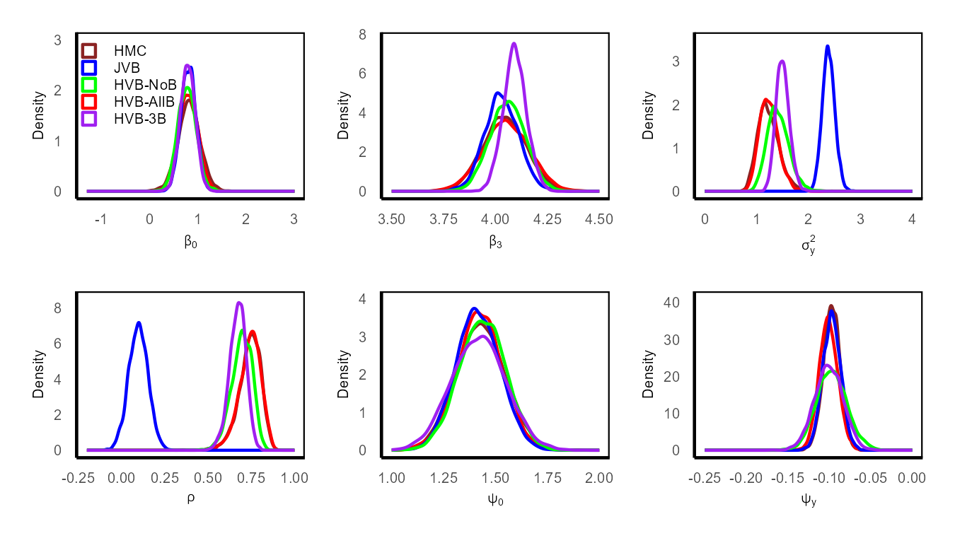
Refer to caption
Figure 3: Posterior densities of SEM and missing data model parameters under MNAR for the simulated dataset with n=625𝑛625n=625 and nu=469subscript𝑛𝑢469n_{u}=469 (around 75%percent7575\% missing) estimated using the HMC, JVB, HVB-NoB, HVB-AllB, and HVB-3B methods
Refer to caption
(a) Posterior means
Refer to caption
(b) Posterior standard deviations
Figure 4: Comparison of the posterior means and standard deviations of missing values from the JVB, HVB-NoB, HVB-AllB, and HVB-3B methods with those obtained using the HMC method under MNAR for the simulated dataset with n=625𝑛625n=625, and nu=469subscript𝑛𝑢469n_{u}=469 (around 75%percent7575\% missing)

Figure 4 compares the posterior means and standard deviations of missing values obtained from the JVB method and all three HVB methods with the HMC method for the simulated dataset with n=625𝑛625n=625 and nu=469subscript𝑛𝑢469n_{u}=469. The JVB posterior means and all the HVB posterior means are very close to those of HMC, as shown in Figure 4(a). However, the posterior standard deviations estimated from the JVB method are significantly different from those obtained from the HMC method, as shown in Figure 4(b), whereas the posterior standard deviations from all the HVB methods closely align with those of HMC.

Similar to SEM under MAR, we also conducted a simulation study with n=10,000𝑛10000n=10,000 with approximately 75%percent7575\% of missing values under MNAR. As implementing HMC is infeasible for large n𝑛n (refer to Table 5), we implement the JVB, HVB-AllB, and HVB-3B methods on this dataset and compare the estimated posterior means of parameters obtained from VB methods with the true parameter values in Table 4. The HVB-NoB algorithm is not implemented due to its high computational cost (as shown in Table 5). The posterior means obtained by HVB-AllB and HVB-3B algorithms accurately estimate the true parameter values, demonstrating superior accuracy compared to the JVB algorithm. See Figures S7 and S8 in Section S5.2 of the online supplement for a comparison of posterior densities of model parameters and a comparison of estimated missing values from the three VB methods with the true missing values, respectively.

True value JVB HVB-AllB HVB-3B
β0=2subscript𝛽02\beta_{0}=2 2.0190 (0.0358) 1.9849 (0.0494) 1.9973 (0.0547)
β3=5subscript𝛽35\beta_{3}=5 5.0077 (0.0247) 5.0118 (0.0214) 4.9898 (0.0081)
σy2=1subscriptsuperscript𝜎2y1\sigma^{2}_{\textbf{y}}=1 2.1769 (0.0441) 0.9682 (0.0286) 0.9209 (0.0152)
ρ=0.8𝜌0.8\rho=0.8 0.1443 (0.0129) 0.8128 (0.0100) 0.8190 (0.0066)
ψ0=1.5subscript𝜓01.5\psi_{0}=1.5 1.5062 (0.0255) 1.5042 (0.0285) 1.5158 (0.0280)
ψk=0.5subscript𝜓𝑘0.5\psi_{k}=0.5 0.5058 (0.0261) 0.4987 (0.0301) 0.5114 (0.0293)
ψy=0.1subscript𝜓y0.1\psi_{\textbf{y}}=-0.1 -0.1003 (0.0057) -0.1098 (0.0090) -0.1002 (0.0083)
Table 4: Posterior means and standard deviations (inside brackets) of SEM and missing data model parameters under MNAR estimated using the JVB and different HVB methods for the simulated dataset with n=10,000𝑛10000n=10,000 and nu=7,542subscript𝑛𝑢7542n_{u}=7,542 (around 75%percent7575\% missing values)
n𝑛n n=625𝑛625n=625 n=1024𝑛1024n=1024 n=2500𝑛2500n=2500
missing percentage 25%percent2525\% 50%percent5050\% 75%percent7575\% 25%percent2525\% 50%percent5050\% 75%percent7575\% 25%percent2525\% 50%percent5050\% 75%percent7575\%
HMC 28.79 32.31 36.22 42.79 98.59 157.52 1046.23 1100.89 1597.88
JVB 0.03 0.04 0.04 0.06 0.07 0.09 0.30 0.38 0.47
HVB-NoB 0.05 0.07 0.07 0.07 0.12 0.20 0.36 0.88 1.91
HVB-AllB 0.25 0.23 0.29 0.31 0.36 0.43 0.66 1.38 1.60
HVB-3B 0.18 0.19 0.20 0.23 0.26 0.30 0.59 0.60 0.67
n𝑛n n=5,041𝑛5041n=5,041 n=7,569𝑛7569n=7,569 n=10,000𝑛10000n=10,000
missing percentage 25%percent2525\% 50%percent5050\% 75%percent7575\% 25%percent2525\% 50%percent5050\% 75%percent7575\% 25%percent2525\% 50%percent5050\% 75%percent7575\%
HMC - - - - - - - - -
JVB 1.34 1.59 2.02 3.52 4.16 5.29 9.23 9.33 13.35
HVB-NoB 1.71 7.29 19.31 4.90 26.62 90.57 11.543 71.82 228.29
HVB-AllB 2.88 3.72 5.43 5.87 8.57 14.54 12.13 17.05 26.29
HVB-3B 1.74 1.98 2.50 4.07 4.95 6.60 9.03 10.53 15.47
Table 5: Average computing time (in seconds) of one iteration of the HMC, JVB, HVB-NoB, HVB-AllB, and HVB-3B methods for estimating SEM under MNAR for different n𝑛n and different missing value (nusubscript𝑛𝑢n_{u}) percentages. For HVB-AllB and HVB-3B, the tuning parameters, such as the block size and the number of MCMC iterations, are set according to the criteria described at the beginning of Section 4.2

Table 5 presents the average computing time (in seconds) per iteration for the VB and HMC methods across different values of n𝑛n and nusubscript𝑛𝑢n_{u} under MNAR. Regardless of the values of n𝑛n and nusubscript𝑛𝑢n_{u}, the HMC method is much more computationally expensive compared to the VB methods. Despite its limitations in accurately capturing the posterior distributions of σy2subscriptsuperscript𝜎2y\sigma^{2}_{\textbf{y}} and ρ𝜌\rho (see Figure 3 and Figure S7 in Section S5.2 of the online supplement), and the posterior standard deviations of missing values (see Figure 4), the JVB method is faster than the any of HVB methods. For smaller values of n𝑛n and nusubscript𝑛𝑢n_{u}, the HVB-NoB algorithm is significantly faster than its counterparts, HVB-AllB and HVB-3B. However, as n𝑛n and nusubscript𝑛𝑢n_{u} increase, the HVB-AllB and HVB-3B are faster than HVB-NoB, with HVB-3B exhibiting the lowest computing cost, as expected.

5 Real example

We utilise the proposed VB methods to analyse a dataset containing votes cast during the 1980 presidential election across 3,107 U.S. counties. This dataset is available in the R package spData  (Bivand et al.,, 2023). The dataset includes county-level information on the following: the proportion of votes cast by the eligible population, the proportion of the eligible population with college degrees, the proportion of the eligible population that owns homes, and income per capita. Pace and Barry, (1997) applied the SDM to this dataset, choosing the logarithm of the proportion of votes cast as the dependent variable. Furthermore, the dataset contains a pre-defined county-level weight matrix, with an average of 5-6 neighbours per unit (county). The weight matrix from the dataset is denser than those used in our simulation studies, which has an average of only 3-4 neighbours per unit. Therefore, implementing VB algorithms for this dataset requires more computing time than the simulation studies.

In our analysis, we treat the logarithm of the proportion of votes cast as the dependent variable. Additionally, we include the logarithms of the proportions of college degrees and homeownership, as well as income per capita, along with their interaction effects, as the set of covariates. Each covariate is standardized to have a mean of zero and a standard deviation of one.

5.1 SEM under MAR

This section investigates the performance of VB methods to estimate SEM under MAR for the 1980 presidential election dataset. Given the full dataset, we randomly select nosubscript𝑛𝑜n_{o} units to form the observed dataset. The remaining nusubscript𝑛𝑢n_{u} units are treated as missing responses. We estimate SEM parameters and the missing values using the JVB and HVB-G algorithms. Due to the moderately large number of observations n=3,107𝑛3107n=3,107, employing the HMC algorithm becomes computationally intensive, as detailed in Table S2 in Section S4.1 of the online supplement. We compare the posterior mean estimates of the SEM parameters with those obtained from the marginal maximum likelihood (ML) method of Suesse, (2018).

For both VB algorithms, we used the starting values as described in the simulation study in Section 4 and ran the algorithms for 15,0001500015,000 iterations, at which point both algorithms were well-converged (see Section S7.2.1 of the online supplement for further details). For the HVB-G algorithm, we set the block size to 500500500 and the number of Gibbs iterations N1subscript𝑁1N_{1} to 101010.

Figure S9 in Section S6.1 of the online supplement presents the posterior densities of the SEM parameters estimated using the JVB and HVB-G methods with 75%percent7575\% missing responses (nu=2,330subscript𝑛𝑢2330n_{u}=2,330). The vertical lines indicate marginal ML estimates. The figure shows that the JVB method yields different posterior density estimates for the parameters σy2subscriptsuperscript𝜎2y\sigma^{2}_{\textbf{y}} and ρ𝜌\rho compared to the HVB-G method. However, the posterior mean estimates of SEM parameters, obtained using the HVB-G method, closely align with the marginal ML estimates compared to those obtained from the JVB method. See Table 6 for a summary of the estimation results.

Figure S10 in Section S6.1 of the online supplement compares the posterior means of missing values obtained from the JVB and HVB-G algorithms with the true missing values. It is evident that the posterior mean estimates of missing values from HVB-G are slightly closer to the true missing values than those from the JVB algorithm; see mean squared errors (MSEs) of estimated missing values in Table 6.

Table 6: Marginal ML estimates (with standard errors in brackets), and posterior means (with posterior standard deviations in brackets) of SEM parameters estimated by JVB and HVB-G algorithms for the 1980 presidential election dataset with 75%percent7575\% (nu=2,330subscript𝑛𝑢2330n_{u}=2,330) missing values under MAR. The table also includes the MSE of missing values obtained from the JVB and HVB algorithms, along with computing time
marginal ML JVB HVB-G
intercept𝑖𝑛𝑡𝑒𝑟𝑐𝑒𝑝𝑡intercept -0.5723 (0.01087) -0.5697 (0.0051) -0.5696 (0.0091)
σy2subscriptsuperscript𝜎2y\sigma^{2}_{\textbf{y}} 0.0089 (0.0006) 0.0253 (0.0007) 0.0093 (0.0006)
ρ𝜌\rho 0.8306 (0.0181) 0.1916 (0.0282) 0.8346 (0.0182)
MSE - 44.8966 32.9627
Computing time in seconds 277.26 10546.5 36939

Table 6 presents the marginal ML estimates with their standard errors and the posterior means and standard deviations of the SEM parameters estimated by the two VB methods. The table also includes the computing time of each algorithm and the MSEs of estimated missing values from JVB and HVB. The table shows that the MSE of HVB-G is lower than that of JVB. See Table S3 in Section S6.1 of the online supplement for further details on the estimation results, including estimates for all the fixed effects.

5.2 SEM under MNAR

This section investigates the performance of VB methods to estimate SEM under MNAR for the 1980 presidential election dataset. The logistic regression in Section 4 is used as the missing data model. We use the logarithms of the proportions of college degrees and the response variable y𝑦y of the SEM (logarithm of the proportion of votes cast) as the covariates in the missing data model. The missing data model has three parameters, denoted as 𝝍=(ψ0,ψx,ψy)𝝍subscript𝜓0subscript𝜓superscriptxsubscript𝜓y\boldsymbol{\psi}=(\psi_{0},\psi_{\textbf{x}^{*}},\psi_{\textbf{y}}). We set the values ψ0=1.4subscript𝜓01.4\psi_{0}=1.4, ψx=0.5subscript𝜓superscriptx0.5\psi_{\textbf{x}^{*}}=0.5, and ψy=0.1subscript𝜓y0.1\psi_{\textbf{y}}=-0.1, resulting in approximately 80%percent8080\% of responses being missing (nu=2,477subscript𝑛𝑢2477n_{u}=2,477).

The JVB, HVB-AllB, and HVB-3B methods are used to estimate the posterior densities of SEM and missing data model parameters. The starting values for all algorithms are chosen similarly to those in the simulation study. The tuning parameters for HVB-AllB and HVB-3B are selected as follows: the number of MCMC iterations is set to N1=20subscript𝑁120N_{1}=20, and since nu>1,000subscript𝑛𝑢1000n_{u}>1,000, the block size ksuperscript𝑘k^{*} is set to nu×10%247subscript𝑛𝑢percent10247n_{u}\times 10\%\approx 247. This led to a total of 11 blocks. All VB algorithms were run for 15,0001500015,000 iterations, at which point all algorithms had well converged. See Figure S24 in Section S7.2.2 of the online supplement for the convergence analysis.

Figure S11 in Section S6.2 of the online supplement compares the posterior densities of SEM and missing data model parameters obtained from the three VB methods. The figure shows that the posterior densities of the parameters, except for σy2subscriptsuperscript𝜎2y\sigma^{2}_{\textbf{y}} and ρ𝜌\rho, obtained from different methods, are almost identical. For σy2subscriptsuperscript𝜎2y\sigma^{2}_{\textbf{y}} and ρ𝜌\rho, the posterior densities obtained from HVB-AllB and HVB-3B are closer to each other compared to those from JVB.

Figure S12 in Section S6.2 of the online supplement compares the posterior means of missing values obtained from the JVB, HVB-AllB, and HVB-3B methods with the true missing values. The posterior means of the missing values obtained from the HVB-AllB method are slightly closer to the true missing values than those from the HVB-3B and JVB algorithms, as indicated by their greater concentration along the diagonal line. This is further supported by the lower MSE of estimated missing values from the HVB-AllB method in comparison to both the HVB-3B and JVB methods, as shown in Table 7. The table also includes the posterior means and standard deviations of parameters obtained from the three VB algorithms, the true parameter values for the missing data model parameters, and the computing time for each method. Although the HVB-3B estimates of missing values have a slightly higher MSE than HVB-AllB, its computing time is nearly three times shorter. Therefore, HVB-3B is an computationally less expensive yet reasonably accurate alternative to the HVB-AllB method. Table S4 in Section S6.2 of the online supplement summarises estimates for all the fixed effects.

Table 7: Posterior means (with posterior standard deviations inside brackets) of SEM and missing data model parameters, and the true parameter values for the missing data model parameters under MNAR obtained from the JVB, HVB-AllB, and HVB-3B methods for the 1980 presidential election datase with approximately 80%percent8080\% missing values (nu=2,477subscript𝑛𝑢2477n_{u}=2,477). The table also includes the MSE of missing values by JVB and HVB algorithms, along with computing time
True value JVB HVB-AllB HVB-3B
intercept(β0)𝑖𝑛𝑡𝑒𝑟𝑐𝑒𝑝𝑡subscript𝛽0intercept~{}(\beta_{0}) NA -0.5815 (0.0112) -0.5773 (0.0163) -0.5689 (0.0078)
σy2subscriptsuperscript𝜎2y\sigma^{2}_{\textbf{y}} NA 0.0242 (0.0006) 0.0109 (0.0008) 0.0154 (0.0006)
ρ𝜌\rho NA 0.1634 (0.0259) 0.8004 (0.0171) 0.6990 (0.0186)
ψ0subscript𝜓0\psi_{0} 1.4 1.6622 (0.1977) 1.6504 (0.1934) 1.5891 (0.1455)
ψxsubscript𝜓superscriptx\psi_{\textbf{x}^{*}} 0.5 0.5227 (0.0519) 0.5172 (0.0497) 0.5376 (0.0454)
ψysubscript𝜓y\psi_{\textbf{y}} -0.1 0.3540 (0.3252) 0.3316 (0.3269) 0.2286 (0.2354)
MSE NA 46.9063 35.7157 37.6031
Computational time in seconds NA 11620.5 68035.5 23787

6 Conclusion

Our article proposes VB methods for estimating SEM under missing at random (MAR) and missing not at random (MNAR) missing data mechanisms. The joint VB (JVB) and the class of hybrid VB (HVB) methods are proposed. The posterior densities estimated using the Hamiltonian Monte Carlo (HMC) method are considered as ground truth to assess the accuracy of the VB methods for a small to moderate number of observations n𝑛n and missing response values nusubscript𝑛𝑢n_{u}. The HMC method for this model is infeasible when n𝑛n and nusubscript𝑛𝑢n_{u} are large.

The empirical results show that: (1) All proposed VB methods are computationally less expensive compared to the HMC method; (2) All HVB methods produce posterior density estimates for all model parameters and missing response values that are similar to those obtained using the HMC method for estimating SEM under MAR and MNAR. However, as n𝑛n and nusubscript𝑛𝑢n_{u} increase, HVB-NoB produces inaccurate estimates due to the low acceptance percentage of the underlying MCMC steps; (3) The HVB-3B method generates slightly different posterior estimates compared to other HVB algorithms. This is expected because, for each MCMC step of the HVB-3B algorithm, updates are performed on only randomly selected 3 blocks; (4) HVB-3B is more scalable for large n𝑛n and nusubscript𝑛𝑢n_{u} compared to HVB-AllB while still providing nearly similar posterior density estimates; (5) The JVB method yields quite accurate posterior density estimates for fixed effect parameters and the posterior means of the missing response values. However, it provides inaccurate posterior density estimates for the parameters σy2subscriptsuperscript𝜎2𝑦\sigma^{2}_{y} and ρ𝜌\rho, as well as for the posterior standard deviations of the missing response values under both MAR and MNAR; (6) Generally, all HVB algorithms tend to converge in fewer iterations compared to the JVB algorithm.

Statements and Declarations

The authors declare no potential or apparent conflict of interest in this article.

References

  • Allison, (2001) Allison, P. D. (2001). Missing data. Sage publications.
  • Anselin, (1988) Anselin, L. (1988). Spatial econometrics: methods and models, volume 4. Springer Science & Business Media.
  • Bansal et al., (2021) Bansal, P., Krueger, R., and Graham, D. J. (2021). Fast Bayesian estimation of spatial count data models. Computational Statistics & Data Analysis, 157:107152.
  • Benedetti et al., (2020) Benedetti, R., Suesse, T., and Piersimoni, F. (2020). Spatial auto-correlation and auto-regressive models estimation from sample survey data. Biometrical Journal, 62(6):1494–1507.
  • Bivand et al., (2023) Bivand, R., Nowosad, J., and Lovelace, R. (2023). spData: Datasets for spatial analysis. R package version 2.2.2.
  • Blei and Jordan, (2006) Blei, D. M. and Jordan, M. I. (2006). Variational inference for Dirichlet process mixtures. Bayesian Analysis, 1(1):121 – 143.
  • Blei et al., (2017) Blei, D. M., Kucukelbir, A., and McAuliffe, J. D. (2017). Variational inference: A review for statisticians. Journal of the American Statistical Association, 112(518):859–877.
  • Bottou, (2010) Bottou, L. (2010). Large-scale machine learning with stochastic gradient descent. In Proceedings of COMPSTAT’2010: 19th International Conference on Computational Statistics Paris France, August 22-27, 2010 Keynote, Invited and Contributed Papers, pages 177–186. Springer.
  • Carpenter et al., (2017) Carpenter, B., Gelman, A., Hoffman, M. D., Lee, D., Goodrich, B., Betancourt, M., Brubaker, M. A., Guo, J., Li, P., and Riddell, A. (2017). Stan: A probabilistic programming language. Journal of statistical software, 76.
  • Cassemiro et al., (2007) Cassemiro, F. A., Diniz-Filho, J. A. F., Rangel, T., and Bini, L. M. (2007). Spatial autocorrelation, model selection and hypothesis testing in geographical ecology: Implications for testing metabolic theory in new world amphibians. Neotropical Biology and Conservation, 2(3):119–126.
  • Chappell et al., (2008) Chappell, M. A., Groves, A. R., Whitcher, B., and Woolrich, M. W. (2008). Variational Bayesian inference for a nonlinear forward model. IEEE Transactions on Signal Processing, 57(1):223–236.
  • Dao et al., (2024) Dao, V. H., Gunawan, D., Tran, M.-N., Kohn, R., Hawkins, G. E., and Brown, S. D. (2024). Efficient selection between hierarchical cognitive models: Cross-validation with variational Bayes. Psychological Methods, 29(1):219–241.
  • De Oliveira and Song, (2008) De Oliveira, V. and Song, J. J. (2008). Bayesian analysis of simultaneous autoregressive models. Sankhyā: The Indian Journal of Statistics, Series B (2008-), pages 323–350.
  • Di Salvatore and Ruggeri, (2021) Di Salvatore, J. and Ruggeri, A. (2021). Spatial analysis for political scientists. Italian Political Science Review/Rivista Italiana di Scienza Politica, 51(2):198–214.
  • Doğan and Taşpinar, (2018) Doğan, O. and Taşpinar, S. (2018). Bayesian inference in spatial sample selection models. Oxford Bulletin of Economics and Statistics, 80(1):90–121.
  • Duane et al., (1987) Duane, S., Kennedy, A. D., Pendleton, B. J., and Roweth, D. (1987). Hybrid Monte Carlo. Physics letters B, 195(2):216–222.
  • Flores-Lagunes and Schnier, (2012) Flores-Lagunes, A. and Schnier, K. E. (2012). Estimation of sample selection models with spatial dependence. Journal of Applied Econometrics, 27(2):173–204.
  • Gelfand et al., (1990) Gelfand, A. E., Hills, S. E., Racine-Poon, A., and Smith, A. F. (1990). Illustration of Bayesian inference in normal data models using Gibbs sampling. Journal of the American Statistical Association, 85(412):972–985.
  • Gunawan et al., (2021) Gunawan, D., Kohn, R., and Nott, D. (2021). Variational Bayes approximation of factor stochastic volatility models. International Journal of Forecasting, 37(4):1355–1375.
  • Gunawan et al., (2023) Gunawan, D., Kohn, R., and Nott, D. (2023). Flexible variational Bayes based on a copula of a mixture. Journal of Computational and Graphical Statistics, pages 1–16.
  • Han et al., (2013) Han, S., Liao, X., and Carin, L. (2013). Integrated non-factorized variational inference. Advances in Neural Information Processing Systems, 26.
  • Han et al., (2016) Han, S., Liao, X., Dunson, D., and Carin, L. (2016). Variational Gaussian copula inference. In Artificial Intelligence and Statistics, pages 829–838. PMLR.
  • Harville, (1997) Harville, D. A. (1997). Matrix algebra from a statistician’s perspective. Springer New York.
  • Hoffman et al., (2014) Hoffman, M. D., Gelman, A., et al. (2014). The No-U-Turn sampler: adaptively setting path lengths in Hamiltonian Monte Carlo. J. Mach. Learn. Res., 15(1):1593–1623.
  • Kelley pace and Barry, (1997) Kelley pace, R. and Barry, R. P. (1997). Fast cars. Journal of Statistical Computation and Simulation, 59(2):123–145.
  • Kingma and Welling, (2013) Kingma, D. P. and Welling, M. (2013). Auto-encoding variational Bayes. arXiv preprint arXiv:1312.6114.
  • Leenders, (2002) Leenders, R. T. A. (2002). Modeling social influence through network autocorrelation: constructing the weight matrix. Social Networks, 24(1):21–47.
  • LeSage and Pace, (2009) LeSage, J. and Pace, R. K. (2009). Introduction to spatial econometrics. Chapman and Hall/CRC.
  • LeSage, (1997) LeSage, J. P. (1997). Bayesian estimation of spatial autoregressive models. International Regional Science Review, 20(1-2):113–129.
  • LeSage and Pace, (2004) LeSage, J. P. and Pace, R. K. (2004). Models for spatially dependent missing data. The Journal of Real Estate Finance and Economics, 29(2):233–254.
  • Li et al., (2012) Li, H., Calder, C. A., and Cressie, N. (2012). One-step estimation of spatial dependence parameters: Properties and extensions of the aple statistic. Journal of Multivariate Analysis, 105(1):68–84.
  • Little and Rubin, (2019) Little, R. J. and Rubin, D. B. (2019). Statistical analysis with missing data, volume 793. John Wiley & Sons.
  • Loaiza-Maya et al., (2022) Loaiza-Maya, R., Smith, M. S., Nott, D. J., and Danaher, P. J. (2022). Fast and accurate variational inference for models with many latent variables. Journal of Econometrics, 230(2):339–362.
  • McElreath, (2018) McElreath, R. (2018). Statistical rethinking: A Bayesian course with examples in R and Stan. Chapman and Hall/CRC.
  • Mollalo et al., (2020) Mollalo, A., Vahedi, B., and Rivera, K. M. (2020). GIS-based spatial modeling of COVID-19 incidence rate in the continental United States. Science of the Total Environment, 728:138884.
  • Neal, (1995) Neal, R. (1995). Bayesian learning for neural networks [phd thesis]. Toronto, Ontario, Canada: Department of Computer Science, University of Toronto.
  • Neal et al., (2011) Neal, R. M. et al. (2011). MCMC using Hamiltonian dynamics. Handbook of Markov chain Monte Carlo, 2(11):2.
  • Nott et al., (2012) Nott, D. J., Tan, S. L., Villani, M., and Kohn, R. (2012). Regression density estimation with variational methods and stochastic approximation. Journal of Computational and Graphical Statistics, 21(3):797–820.
  • Ong et al., (2018) Ong, V. M.-H., Nott, D. J., and Smith, M. S. (2018). Gaussian variational approximation with a factor covariance structure. Journal of Computational and Graphical Statistics, 27(3):465–478.
  • Ord, (1975) Ord, K. (1975). Estimation methods for models of spatial interaction. Journal of the American Statistical Association, 70(349):120–126.
  • Ormerod and Wand, (2010) Ormerod, J. T. and Wand, M. P. (2010). Explaining variational approximations. The American Statistician, 64(2):140–153.
  • Pace and Barry, (1997) Pace, R. K. and Barry, R. (1997). Quick computation of spatial autoregressive estimators. Geographical analysis, 29(3):232–247.
  • Poyiadjis et al., (2011) Poyiadjis, G., Doucet, A., and Singh, S. S. (2011). Particle approximations of the score and observed information matrix in state space models with application to parameter estimation. Biometrika, 98(1):65–80.
  • Rabovič and Čížek, (2023) Rabovič, R. and Čížek, P. (2023). Estimation of spatial sample selection models: A partial maximum likelihood approach. Journal of Econometrics, 232(1):214–243.
  • (45) Rezende, D. J., Mohamed, S., and Wierstra, D. (2014a). Stochastic backpropagation and approximate inference in deep generative models. In International Conference on Machine Learning, pages 1278–1286. PMLR.
  • (46) Rezende, D. J., Mohamed, S., and Wierstra, D. (2014b). Stochastic backpropagation and approximate inference in deep generative models. In Xing, E. P. and Jebara, T., editors, Proceedings of the 31st International Conference on Machine Learning, volume 32 of Proceedings of Machine Learning Research, pages 1278–1286, Bejing, China. PMLR.
  • Robbins and Monro, (1951) Robbins, H. and Monro, S. (1951). A stochastic approximation method. The Annals of Mathematical Statistics, pages 400–407.
  • Rubin, (1976) Rubin, D. B. (1976). Inference and missing data. Biometrika, 63(3):581–592.
  • Seya et al., (2021) Seya, H., Tomari, M., and Uno, S. (2021). Parameter estimation in spatial econometric models with non-random missing data. Applied Economics Letters, 28(6):440–446.
  • Stan Development Team, (2020) Stan Development Team (2020). RStan: the R interface to Stan.
  • Stan Development Team, (2023) Stan Development Team (2023). RStan: the R interface to Stan. R package version 2.21.8.
  • Suesse, (2018) Suesse, T. (2018). Marginal maximum likelihood estimation of SAR models with missing data. Computational Statistics & Data Analysis, 120:98–110.
  • Suesse and Zammit-Mangion, (2017) Suesse, T. and Zammit-Mangion, A. (2017). Computational aspects of the EM algorithm for spatial econometric models with missing data. Journal of Statistical Computation and Simulation, 87(9):1767–1786.
  • Tan and Nott, (2018) Tan, L. S. and Nott, D. J. (2018). Gaussian variational approximation with sparse precision matrices. Statistics and Computing, 28:259–275.
  • Titsias and Lázaro-Gredilla, (2015) Titsias, M. and Lázaro-Gredilla, M. (2015). Local expectation gradients for black box variational inference. In Cortes, C., Lawrence, N., Lee, D., Sugiyama, M., and Garnett, R., editors, Advances in Neural Information Processing Systems, volume 28. Curran Associates, Inc.
  • Titsias and Lázaro-Gredilla, (2014) Titsias, M. and Lázaro-Gredilla, M. (2014). Doubly stochastic variational Bayes for non-conjugate inference. In Xing, E. P. and Jebara, T., editors, Proceedings of the 31st International Conference on Machine Learning, volume 32 of Proceedings of Machine Learning Research, pages 1971–1979, Bejing, China. PMLR.
  • Ver Hoef et al., (2018) Ver Hoef, J. M., Peterson, E. E., Hooten, M. B., Hanks, E. M., and Fortin, M.-J. (2018). Spatial autoregressive models for statistical inference from ecological data. Ecological Monographs, 88(1):36–59.
  • Wang and Lee, (2013) Wang, W. and Lee, L.-F. (2013). Estimation of spatial autoregressive models with randomly missing data in the dependent variable. The Econometrics Journal, 16(1):73–102.
  • Wijayawardhana et al., (2024) Wijayawardhana, A., Suesse, T., and Gunawan, D. (2024). Statistical inference on hierarchical simultaneous autoregressive models with missing data. arXiv preprint arXiv:2403.17257.
  • Wong and Li, (2020) Wong, D. W. and Li, Y. (2020). Spreading of COVID-19: Density matters. Plos One, 15(12):e0242398.
  • Wu, (2018) Wu, G. (2018). Fast and scalable variational Bayes estimation of spatial econometric models for Gaussian data. Spatial Statistics, 24:32–53.
  • Xu et al., (2019) Xu, M., Quiroz, M., Kohn, R., and Sisson, S. A. (2019). Variance reduction properties of the reparameterization trick. In The 22nd International Conference on Artificial Intelligence and Statistics, pages 2711–2720. PMLR.
  • Zeiler, (2012) Zeiler, M. D. (2012). Adadelta: An adaptive learning rate method. ArXiv, abs/1212.5701.
  • Zhu et al., (2020) Zhu, X., Huang, D., Pan, R., and Wang, H. (2020). Multivariate spatial autoregressive model for large scale social networks. Journal of Econometrics, 215(2):591–606.

Online Supplement for Variational Bayes Inference for Spatial Error Models with Missing Data

We use the following notation in the online supplement. Eq. (1), Table 1, Figure 1, and Algorithm 1, etc, refer to the main paper, while Eq. (S1), Table S1, Figure S1, and Algorithm S1, etc, refer to the supplement.

S1 Derivation of VB algorithms

S1.1 Derivation of the reparameterisation gradient for JVB algorithm

In the main paper, the reparameterisation gradient of (𝝀)𝝀\mathcal{L}(\boldsymbol{\lambda}) for JVB algorithm is given by

𝝀(𝝀)=Ef𝜻[du(𝜻,𝝀)d𝝀{𝜽,yulogh(𝜽,yu)𝜽,yulogq𝝀(𝜽,yu)}],subscript𝝀𝝀subscript𝐸subscript𝑓𝜻delimited-[]𝑑𝑢superscript𝜻𝝀top𝑑𝝀subscript𝜽subscripty𝑢log𝜽subscripty𝑢subscript𝜽subscripty𝑢logsubscript𝑞𝝀𝜽subscripty𝑢\nabla_{\boldsymbol{\lambda}}\mathcal{L}(\boldsymbol{\lambda})=E_{f_{\boldsymbol{\zeta}}}\left[\frac{du(\boldsymbol{\zeta,\boldsymbol{\lambda}})^{\top}}{d\boldsymbol{\lambda}}\{\nabla_{\boldsymbol{\theta},\textbf{y}_{u}}\text{log}~{}h(\boldsymbol{\theta},\textbf{y}_{u})-\nabla_{\boldsymbol{\theta},\textbf{y}_{u}}\text{log}~{}q_{\boldsymbol{\lambda}}(\boldsymbol{\theta},\textbf{y}_{u})\}\right],\\ (S1)

where du(𝜻,𝝀)d𝝀𝑑𝑢𝜻𝝀𝑑𝝀\frac{du(\boldsymbol{\zeta,\boldsymbol{\lambda}})}{d\boldsymbol{\lambda}} is the derivative of the transformation u(𝜻,𝝀)=𝝁+B𝜼+dϵ𝑢𝜻𝝀𝝁B𝜼dbold-italic-ϵu(\boldsymbol{\zeta,\boldsymbol{\lambda}})=\boldsymbol{\mu}+\textbf{B}\boldsymbol{\eta}+\textbf{d}\circ\boldsymbol{\epsilon} with respect to the variational parameters 𝝀=(𝝁,vech(B),d)𝝀superscriptsuperscript𝝁topvechsuperscriptBtopsuperscriptdtoptop\boldsymbol{\lambda}=(\boldsymbol{\mu}^{\top},\text{vech}(\textbf{B})^{\top},\textbf{d}^{\top})^{\top}, where ”vech” operator is the vectorisation of a matrix by stacking its columns from left to right. We write that u(𝜻,𝝀)=𝝁+(𝜼IS+nu)vech(B)+dϵ𝑢𝜻𝝀𝝁tensor-productsuperscript𝜼topsubscriptI𝑆subscript𝑛𝑢vechBdbold-italic-ϵu(\boldsymbol{\zeta,\boldsymbol{\lambda}})=\boldsymbol{\mu}+(\boldsymbol{\eta}^{\top}\otimes\textbf{I}_{S+n_{u}})\text{vech}(\textbf{B})+\textbf{d}\circ\boldsymbol{\epsilon}, where tensor-product\otimes represents the Kronecker product, and IS+nusubscriptI𝑆subscript𝑛𝑢\textbf{I}_{S+n_{u}} is the identity matrix of size S+nu𝑆subscript𝑛𝑢S+n_{u}. It can be shown that 𝜽,yulogq𝝀(𝜽,yu)=(BB+D2)1((𝜽,yu)𝝁)subscript𝜽subscripty𝑢logsubscript𝑞𝝀𝜽subscripty𝑢superscriptsuperscriptBBtopsuperscriptD21superscriptsuperscript𝜽topsuperscriptsubscripty𝑢toptop𝝁\nabla_{\boldsymbol{\theta},\textbf{y}_{u}}\text{log}~{}q_{\boldsymbol{\lambda}}(\boldsymbol{\theta},\textbf{y}_{u})=-(\textbf{B}\textbf{B}^{\top}+\textbf{D}^{2})^{-1}((\boldsymbol{\theta}^{\top},\textbf{y}_{u}^{\top})^{\top}-\boldsymbol{\mu}),

du(𝜻,𝝀)d𝝁=IS+nuanddu(𝜻,𝝀)dvech(B)=𝜼IS+nu.formulae-sequence𝑑𝑢𝜻𝝀𝑑𝝁subscriptI𝑆subscript𝑛𝑢and𝑑𝑢𝜻𝝀𝑑vechBtensor-productsuperscript𝜼topsubscriptI𝑆subscript𝑛𝑢\frac{du(\boldsymbol{\zeta},\boldsymbol{\lambda})}{d\boldsymbol{\mu}}=\textbf{I}_{S+n_{u}}\\ ~{}~{}~{}~{}~{}\text{and}~{}~{}~{}~{}~{}\frac{du(\boldsymbol{\zeta},\boldsymbol{\lambda})}{d\text{vech}(\textbf{B})}=\boldsymbol{\eta}^{\top}\otimes\textbf{I}_{S+n_{u}}. (S2)

The derivatives of the lower bound with respect to variational parameters are:

𝝁(𝝀)=Ef𝜻[𝜽,yulogh(𝝁+B𝜼+dϵ)+(BB+D2)1(B𝜼+dϵ)],subscript𝝁𝝀subscript𝐸subscript𝑓𝜻delimited-[]subscript𝜽subscripty𝑢log𝝁B𝜼dbold-italic-ϵsuperscriptsuperscriptBBtopsuperscriptD21B𝜼dbold-italic-ϵ\begin{split}\nabla_{\boldsymbol{\mu}}\mathcal{L}(\boldsymbol{\lambda})&=E_{f_{\boldsymbol{\zeta}}}[\nabla_{\boldsymbol{\theta},\textbf{y}_{u}}~{}\text{log}~{}h(\boldsymbol{\mu}+\textbf{B}\boldsymbol{\eta}+\textbf{d}\circ\boldsymbol{\epsilon})\\ &+(\textbf{B}\textbf{B}^{\top}+\textbf{D}^{2})^{-1}(\textbf{B}\boldsymbol{\eta}+\textbf{d}\circ\boldsymbol{\epsilon})],\end{split} (S3)
B(𝝀)=Ef𝜻[𝜽,yulogh(𝝁+B𝜼+dϵ)𝜼+(BB+D2)1(B𝜼+dϵ)𝜼],subscriptB𝝀subscript𝐸subscript𝑓𝜻delimited-[]subscript𝜽subscripty𝑢log𝝁B𝜼dbold-italic-ϵsuperscript𝜼topsuperscriptsuperscriptBBtopsuperscriptD21B𝜼dbold-italic-ϵsuperscript𝜼top\begin{split}\nabla_{\textbf{B}}\mathcal{L}(\boldsymbol{\lambda})&=E_{f_{\boldsymbol{\zeta}}}[\nabla_{\boldsymbol{\theta},\textbf{y}_{u}}\text{log}~{}h(\boldsymbol{\mu}+\textbf{B}\boldsymbol{\eta}+\textbf{d}\circ\boldsymbol{\epsilon})\boldsymbol{\eta}^{\top}\\ &+(\textbf{B}\textbf{B}^{\top}+\textbf{D}^{2})^{-1}(\textbf{B}\boldsymbol{\eta}+\textbf{d}\circ\boldsymbol{\epsilon})\boldsymbol{\eta}^{\top}],\end{split} (S4)

and

d(𝝀)=Ef𝜻[diag(𝜽,yulogh(𝝁+B𝜼+dϵ)ϵ+(BB+D2)1(B𝜼+dϵ)ϵ)],subscriptd𝝀subscript𝐸subscript𝑓𝜻delimited-[]diagsubscript𝜽subscripty𝑢log𝝁B𝜼dbold-italic-ϵsuperscriptbold-italic-ϵtopsuperscriptsuperscriptBBtopsuperscriptD21B𝜼dbold-italic-ϵsuperscriptbold-italic-ϵtop\begin{split}\nabla_{\textbf{d}}\mathcal{L}(\boldsymbol{\lambda})&=E_{f_{\boldsymbol{\zeta}}}[\text{diag}(\nabla_{\boldsymbol{\theta},\textbf{y}_{u}}\text{log}~{}h(\boldsymbol{\mu}+\textbf{B}\boldsymbol{\eta}+\textbf{d}\circ\boldsymbol{\epsilon})\boldsymbol{\epsilon}^{\top}\\ &+(\textbf{B}\textbf{B}^{\top}+\textbf{D}^{2})^{-1}(\textbf{B}\boldsymbol{\eta}+\textbf{d}\circ\boldsymbol{\epsilon})\boldsymbol{\epsilon}^{\top})],\end{split} (S5)

where diag()diag\text{diag}(\cdot) is the vector of diagonal elements extracted from a square matrix. The analytical expressions for 𝜽,yulogh(𝝁+B𝜼+dϵ)=𝜽,yulogh(𝜽,yu)subscript𝜽subscripty𝑢log𝝁B𝜼dbold-italic-ϵsubscript𝜽subscripty𝑢log𝜽subscripty𝑢\nabla_{\boldsymbol{\theta},\textbf{y}_{u}}\text{log}~{}h(\boldsymbol{\mu}+\textbf{B}\boldsymbol{\eta}+\textbf{d}\circ\boldsymbol{\epsilon})=\nabla_{\boldsymbol{\theta},\textbf{y}_{u}}\text{log}~{}h(\boldsymbol{\theta},\textbf{y}_{u}) in Equations (S3)-(S5) under MAR and MNAR mechanisms are provided in Section S2. The expectations in these gradients can be estimated using a single sample drawn from f𝜻subscript𝑓𝜻f_{\boldsymbol{\zeta}}, and they provide unbiased estimates 𝝀(𝝀)^^subscript𝝀𝝀\widehat{{\nabla_{\boldsymbol{\lambda}}\mathcal{L}(\boldsymbol{\lambda})}} for 𝝀(𝝀)subscript𝝀𝝀\nabla_{\boldsymbol{\lambda}}\mathcal{L}(\boldsymbol{\lambda}). These estimates are utilised in the gradient calculation step (step 4) of Algorithm 1 of the main paper. The adaptive learning rates (step sizes) utilised in Algorithm 1 are determined through the ADADELTA algorithm  (Zeiler,, 2012), as detailed in Section S1.3.

Computing gradient estimates using Equations (S3), (S4), and (S5) presents computational problems, in particular, when number of covariates and missing values is large. The inversion of (S+nu)×(S+nu)𝑆subscript𝑛𝑢𝑆subscript𝑛𝑢(S+n_{u})\times(S+n_{u}) matrix, (BBT+D2)superscriptBB𝑇superscriptD2(\textbf{B}\textbf{B}^{T}+\textbf{D}^{2}), is computationally expensive. Using the Woodbury formula (Harville,, 1997, p. 427), this inversion can be reformulated as:

(BBT+D2)1=D2D2B(Ip+BTD2B)1BTD2,superscriptsuperscriptBB𝑇superscriptD21superscriptD2superscriptD2BsuperscriptsubscriptI𝑝superscriptB𝑇superscript𝐷2B1superscriptB𝑇superscriptD2(\textbf{B}\textbf{B}^{T}+\textbf{D}^{2})^{-1}=\textbf{D}^{-2}-\textbf{D}^{-2}\textbf{B}(\textbf{I}_{p}+\textbf{B}^{T}D^{-2}\textbf{B})^{-1}\textbf{B}^{T}\textbf{D}^{-2}, (S6)

where IpsubscriptI𝑝\textbf{I}_{p} is the diagonal matrix of dimension p×p𝑝𝑝p\times p.

On the right-hand side of Equation (S6), the term (Ip+BTD2B)subscriptI𝑝superscriptB𝑇superscriptD2B(\textbf{I}_{p}+\textbf{B}^{T}\textbf{D}^{-2}\textbf{B}) is a square matrix of size p×p𝑝𝑝p\times p (where p𝑝p is much smaller than S+nu𝑆subscript𝑛𝑢S+n_{u}), and D is a diagonal matrix. Directly inverting (I+BTD2B)IsuperscriptB𝑇superscriptD2B(\textbf{I}+\textbf{B}^{T}\textbf{D}^{-2}\textbf{B}) has a computational complexity of O(p3)𝑂superscript𝑝3O(p^{3}). Consequently, computing (BBT+D2)1superscriptsuperscriptBB𝑇superscriptD21(\textbf{B}\textbf{B}^{T}+\textbf{D}^{2})^{-1} using this method also involves O(p3)𝑂superscript𝑝3O(p^{3}) complexity. Alternatively, without utilising the Woodbury formula, the complexity increases significantly to O((S+nu)3)𝑂superscript𝑆subscript𝑛𝑢3O((S+n_{u})^{3}).

S1.2 Derivation of the reparameterisation gradient for HVB algorithm

Since (𝝀)=Eq(logp(O𝜽)+logp(𝜽)logq𝝀0(𝜽))=0(𝝀)𝝀subscript𝐸𝑞log𝑝conditionalO𝜽log𝑝𝜽logsuperscriptsubscript𝑞𝝀0𝜽superscript0𝝀\mathcal{L}(\boldsymbol{\lambda})=E_{q}\left(\text{log}~{}p(\textbf{O}\mid\boldsymbol{\theta})+\text{log}~{}p(\boldsymbol{\theta})-\text{log}~{}q_{\boldsymbol{\lambda}}^{0}(\boldsymbol{\theta})\right)=\mathcal{L}^{0}(\boldsymbol{\lambda}) as shown in Section 3.3 of the main paper, the reparameterisation gradient of \mathcal{L} is the same as that of 0superscript0\mathcal{L}^{0},

𝝀(𝝀)=Ef𝜹0[dt0(𝜹0,𝝀𝜽)d𝝀𝜽(𝜽logp(𝜽)+𝜽logp(O𝜽)𝜽logq𝝀0(𝜽))],subscript𝝀𝝀subscript𝐸subscript𝑓superscript𝜹0delimited-[]𝑑superscript𝑡0superscriptsuperscript𝜹0subscript𝝀𝜽top𝑑subscript𝝀𝜽subscript𝜽log𝑝𝜽subscript𝜽log𝑝conditionalO𝜽subscript𝜽logsuperscriptsubscript𝑞𝝀0𝜽\nabla_{\boldsymbol{\lambda}}\mathcal{L}(\boldsymbol{\lambda})=E_{f_{\boldsymbol{\delta}^{0}}}\left[\frac{dt^{0}(\boldsymbol{\delta}^{0},\boldsymbol{\lambda}_{\boldsymbol{\theta}})^{\top}}{d\boldsymbol{\lambda_{\boldsymbol{\theta}}}}(\nabla_{\boldsymbol{\theta}}\text{log}~{}p(\boldsymbol{\theta})+\nabla_{\boldsymbol{\theta}}\text{log}~{}p(\textbf{O}\mid\boldsymbol{\theta})-\nabla_{\boldsymbol{\theta}}\text{log}~{}q_{\boldsymbol{\lambda}}^{0}(\boldsymbol{\theta}))\right], (S7)

where, the random vector 𝜹0superscript𝜹0\boldsymbol{\delta}^{0} has density f𝜹0subscript𝑓superscript𝜹0f_{\boldsymbol{\delta}^{0}}, which follows a standard normal, and does not depend on 𝝀𝜽subscript𝝀𝜽\boldsymbol{\lambda_{\boldsymbol{\theta}}}, and t0superscript𝑡0t^{0} is the one-to-one vector-valued transformation from 𝜹0=(𝜼0,ϵ0)superscript𝜹0superscriptsuperscriptsuperscript𝜼0topsuperscriptsuperscriptbold-italic-ϵ0toptop\boldsymbol{\delta}^{0}=({\boldsymbol{\eta}^{0}}^{\top},{\boldsymbol{\epsilon}^{0}}^{\top})^{\top} to the parameter vector, such that 𝜽=t0(𝜹0,𝝀𝜽)=𝝁𝜽+B𝜽𝜼0+d𝜽ϵ0𝜽superscript𝑡0superscript𝜹0subscript𝝀𝜽subscript𝝁𝜽subscriptB𝜽superscript𝜼0subscriptd𝜽superscriptbold-italic-ϵ0\boldsymbol{\theta}=t^{0}(\boldsymbol{\delta}^{0},\boldsymbol{\lambda}_{\boldsymbol{\theta}})=\boldsymbol{\mu}_{\boldsymbol{\theta}}+\textbf{B}_{\boldsymbol{\theta}}\boldsymbol{\eta}^{0}+\textbf{d}_{\boldsymbol{\theta}}\circ\boldsymbol{\epsilon}^{0}.

The Fisher’s identity is given by

𝜽logp(O𝜽)=𝜽[log(p(Oyu,𝜽)p(yu𝜽))]p(yuO,𝜽)𝑑yu,subscript𝜽log𝑝conditionalO𝜽subscript𝜽log𝑝conditionalOsubscripty𝑢𝜽𝑝conditionalsubscripty𝑢𝜽𝑝conditionalsubscripty𝑢O𝜽differential-dsubscripty𝑢\nabla_{\boldsymbol{\theta}}\text{log}~{}p(\textbf{O}\mid\boldsymbol{\theta})=\int\nabla_{\boldsymbol{\theta}}\left[\text{log}~{}(p(\textbf{O}\mid\textbf{y}_{u},\boldsymbol{\theta})p(\textbf{y}_{u}\mid\boldsymbol{\theta}))\right]p(\textbf{y}_{u}\mid\textbf{O},\boldsymbol{\theta})d\textbf{y}_{u}, (S8)

see, for example, Poyiadjis et al., (2011).

Substituting this expression into Equation (S7), and writing Ef𝜹()subscript𝐸subscript𝑓𝜹E_{f_{\boldsymbol{\delta}}}(\cdot) for expectation with respect to f𝜹(𝜹)=f𝜹0(𝜹0)p(yu𝜽,O)subscript𝑓𝜹𝜹subscript𝑓superscript𝜹0superscript𝜹0𝑝conditionalsubscripty𝑢𝜽Of_{\boldsymbol{\delta}}(\boldsymbol{\delta})=f_{\boldsymbol{\delta}^{0}}(\boldsymbol{\delta}^{0})p(\textbf{y}_{u}\mid\boldsymbol{\theta},\textbf{O}) and because h(𝜽,yu)=p(Oyu,𝜽)p(yu𝜽)p(𝜽)𝜽subscripty𝑢𝑝conditionalOsubscripty𝑢𝜽𝑝conditionalsubscripty𝑢𝜽𝑝𝜽h(\boldsymbol{\theta},\textbf{y}_{u})=p(\textbf{O}\mid\textbf{y}_{u},\boldsymbol{\theta})p(\textbf{y}_{u}\mid\boldsymbol{\theta})p(\boldsymbol{\theta}), we get

𝝀(𝝀)=Ef𝜹[dt0(𝜹0,𝝀𝜽)d𝝀𝜽(𝜽logp(𝜽)+𝜽logp(y𝒖𝜽)+𝜽logp(Oyu,𝜽)𝜽logq𝝀0(𝜽))]=Ef𝜹[dt0(𝜹0,𝝀𝜽)d𝝀𝜽(𝜽logh(𝜽,yu)𝜽logq𝝀0(𝜽))].subscript𝝀𝝀subscript𝐸subscript𝑓𝜹delimited-[]𝑑superscript𝑡0superscriptsuperscript𝜹0subscript𝝀𝜽top𝑑subscript𝝀𝜽subscript𝜽log𝑝𝜽subscript𝜽log𝑝conditionalsubscripty𝒖𝜽subscript𝜽log𝑝conditionalOsubscripty𝑢𝜽subscript𝜽logsuperscriptsubscript𝑞𝝀0𝜽subscript𝐸subscript𝑓𝜹delimited-[]𝑑superscript𝑡0superscriptsuperscript𝜹0subscript𝝀𝜽top𝑑subscript𝝀𝜽subscript𝜽log𝜽subscripty𝑢subscript𝜽logsuperscriptsubscript𝑞𝝀0𝜽\begin{split}\nabla_{\boldsymbol{\lambda}}\mathcal{L}(\boldsymbol{\lambda})&=E_{f_{\boldsymbol{\delta}}}\left[\frac{dt^{0}(\boldsymbol{\delta}^{0},\boldsymbol{\lambda}_{\boldsymbol{\theta}})^{\top}}{d\boldsymbol{\lambda_{\boldsymbol{\theta}}}}(\nabla_{\boldsymbol{\theta}}\text{log}~{}p(\boldsymbol{\theta})+\nabla_{\boldsymbol{\theta}}\text{log}~{}p(\boldsymbol{\textbf{y}_{u}\mid\theta})+\nabla_{\boldsymbol{\theta}}\text{log}~{}p(\textbf{O}\mid\textbf{y}_{u},\boldsymbol{\theta})-\nabla_{\boldsymbol{\theta}}\text{log}~{}q_{\boldsymbol{\lambda}}^{0}(\boldsymbol{\theta}))\right]\\ &=E_{f_{\boldsymbol{\delta}}}\left[\frac{dt^{0}(\boldsymbol{\delta}^{0},\boldsymbol{\lambda}_{\boldsymbol{\theta}})^{\top}}{d\boldsymbol{\lambda_{\boldsymbol{\theta}}}}(\nabla_{\boldsymbol{\theta}}\text{log}~{}h(\boldsymbol{\theta},\textbf{y}_{u})-\nabla_{\boldsymbol{\theta}}\text{log}~{}q_{\boldsymbol{\lambda}}^{0}(\boldsymbol{\theta}))\right].\\ \end{split} (S9)

The term dt0(𝜹0,𝝀𝜽)d𝝀𝜽𝑑superscript𝑡0superscript𝜹0subscript𝝀𝜽𝑑subscript𝝀𝜽\frac{dt^{0}(\boldsymbol{\delta}^{0},\boldsymbol{\lambda}_{\boldsymbol{\theta}})}{d\boldsymbol{\lambda_{\boldsymbol{\theta}}}} in Equation (S9) is the derivative of the transformation t0(𝜹0,𝝀𝜽)=𝝁𝜽+B𝜽𝜼0+d𝜽ϵ0superscript𝑡0superscript𝜹0subscript𝝀𝜽subscript𝝁𝜽subscriptB𝜽superscript𝜼0subscriptd𝜽superscriptbold-italic-ϵ0t^{0}(\boldsymbol{\delta}^{0},\boldsymbol{\lambda}_{\boldsymbol{\theta}})=\boldsymbol{\mu}_{\boldsymbol{\theta}}+\textbf{B}_{\boldsymbol{\theta}}\boldsymbol{\eta}^{0}+\textbf{d}_{\boldsymbol{\theta}}\circ\boldsymbol{\epsilon}^{0} with respect to the variational parameters 𝝀𝜽=(𝝁𝜽,vech(B𝜽),d𝜽)subscript𝝀𝜽superscriptsuperscriptsubscript𝝁𝜽topvechsuperscriptsubscriptB𝜽topsuperscriptsubscriptd𝜽toptop\boldsymbol{\lambda}_{\boldsymbol{\theta}}=(\boldsymbol{\mu}_{\boldsymbol{\theta}}^{\top},\text{vech}(\textbf{B}_{\boldsymbol{\theta}})^{\top},\textbf{d}_{\boldsymbol{\theta}}^{\top})^{\top}. We can express that t0(𝜹0,𝝀𝜽)=𝝁𝜽+(𝜼0IS)vech(B𝜽)+d𝜽ϵ0superscript𝑡0superscript𝜹0subscript𝝀𝜽subscript𝝁𝜽tensor-productsuperscript𝜼0subscriptI𝑆vechsubscriptB𝜽subscriptd𝜽superscriptbold-italic-ϵ0t^{0}(\boldsymbol{\delta}^{0},\boldsymbol{\lambda}_{\boldsymbol{\theta}})=\boldsymbol{\mu}_{\boldsymbol{\theta}}+(\boldsymbol{\eta}^{0}\otimes\textbf{I}_{S})\text{vech}(\textbf{B}_{\boldsymbol{\theta}})+\textbf{d}_{\boldsymbol{\theta}}\circ\boldsymbol{\epsilon}^{0}, where ISsubscriptI𝑆\textbf{I}_{S} is the identity matrix of size S𝑆S, and it can be further shown that 𝜽logq𝝀0(𝜽)=(B𝜽B𝜽+D𝜽2)1(𝜽𝝁𝜽)subscript𝜽logsubscriptsuperscript𝑞0𝝀𝜽superscriptsubscriptB𝜽superscriptsubscriptB𝜽topsuperscriptsubscriptD𝜽21𝜽subscript𝝁𝜽\nabla_{\boldsymbol{\theta}}\text{log}~{}q^{0}_{\boldsymbol{\lambda}}(\boldsymbol{\theta})=-(\textbf{B}_{\boldsymbol{\theta}}\textbf{B}_{\boldsymbol{\theta}}^{\top}+\textbf{D}_{\boldsymbol{\theta}}^{2})^{-1}(\boldsymbol{\theta}-\boldsymbol{\mu}_{\boldsymbol{\theta}}),

dt0(𝜹0,𝝀𝜽)d𝝁𝜽=ISanddt0(𝜹0,𝝀𝜽)dvech(B𝜽)=𝜼0IS.formulae-sequence𝑑superscript𝑡0superscript𝜹0subscript𝝀𝜽𝑑subscript𝝁𝜽subscriptI𝑆and𝑑superscript𝑡0superscript𝜹0subscript𝝀𝜽𝑑vechsubscriptB𝜽tensor-productsuperscriptsuperscript𝜼0topsubscriptI𝑆\frac{dt^{0}(\boldsymbol{\delta}^{0},\boldsymbol{\lambda}_{\boldsymbol{\theta}})}{d\boldsymbol{\mu}_{\boldsymbol{\theta}}}=\textbf{I}_{S}\\ ~{}~{}~{}~{}~{}\text{and}~{}~{}~{}~{}~{}\frac{dt^{0}(\boldsymbol{\delta}^{0},\boldsymbol{\lambda}_{\boldsymbol{\theta}})}{d\text{vech}(\textbf{B}_{\boldsymbol{\theta}})}={\boldsymbol{\eta}^{0}}^{\top}\otimes\textbf{I}_{S}. (S10)

The derivatives of the lower bound with respect to variational parameters are:

𝝁𝜽(𝝀)=Ef𝜹(𝜽logh(𝝁𝜽+B𝜽𝜼0+d𝜽ϵ0,yu)+(B𝜽B𝜽+D𝜽2)1(B𝜽𝜼0+d𝜽ϵ0)),subscriptsubscript𝝁𝜽𝝀subscript𝐸subscript𝑓𝜹subscript𝜽logsubscript𝝁𝜽subscriptB𝜽superscript𝜼0subscriptd𝜽superscriptbold-italic-ϵ0subscripty𝑢superscriptsubscriptB𝜽superscriptsubscriptB𝜽topsuperscriptsubscriptD𝜽21subscriptB𝜽superscript𝜼0subscriptd𝜽superscriptbold-italic-ϵ0\begin{split}\nabla_{\boldsymbol{\mu}_{\boldsymbol{\theta}}}\mathcal{L}(\boldsymbol{\lambda})&=E_{f_{\boldsymbol{\delta}}}(\nabla_{\boldsymbol{\theta}}~{}\text{log}~{}h(\boldsymbol{\mu}_{\boldsymbol{\theta}}+\textbf{B}_{\boldsymbol{\theta}}\boldsymbol{\eta}^{0}+\textbf{d}_{\boldsymbol{\theta}}\circ\boldsymbol{\epsilon}^{0},\textbf{y}_{u})\\ &+(\textbf{B}_{\boldsymbol{\theta}}\textbf{B}_{\boldsymbol{\theta}}^{\top}+\textbf{D}_{\boldsymbol{\theta}}^{2})^{-1}(\textbf{B}_{\boldsymbol{\theta}}\boldsymbol{\eta}^{0}+\textbf{d}_{\boldsymbol{\theta}}\circ\boldsymbol{\epsilon}^{0})),\end{split} (S11)
B𝜽(𝝀)=Ef𝜹(𝜽logh(𝝁𝜽+B𝜽𝜼0+d𝜽ϵ0,yu)𝜼0+(B𝜽B𝜽+D𝜽2)1(B𝜽𝜼0+d𝜽ϵ0)𝜼0),subscriptsubscriptB𝜽𝝀subscript𝐸subscript𝑓𝜹subscript𝜽logsubscript𝝁𝜽subscriptB𝜽superscript𝜼0subscriptd𝜽superscriptbold-italic-ϵ0subscripty𝑢superscriptsuperscript𝜼0topsuperscriptsubscriptB𝜽superscriptsubscriptB𝜽topsuperscriptsubscriptD𝜽21subscriptB𝜽superscript𝜼0subscriptd𝜽superscriptbold-italic-ϵ0superscriptsuperscript𝜼0top\begin{split}\nabla_{\textbf{B}_{\boldsymbol{\theta}}}\mathcal{L}(\boldsymbol{\lambda})&=E_{f_{\boldsymbol{\delta}}}(\nabla_{\boldsymbol{\theta}}~{}\text{log}~{}h(\boldsymbol{\mu}_{\boldsymbol{\theta}}+\textbf{B}_{\boldsymbol{\theta}}\boldsymbol{\eta}^{0}+\textbf{d}_{\boldsymbol{\theta}}\circ\boldsymbol{\epsilon}^{0},\textbf{y}_{u}){\boldsymbol{\eta}^{0}}^{\top}\\ &+(\textbf{B}_{\boldsymbol{\theta}}\textbf{B}_{\boldsymbol{\theta}}^{\top}+\textbf{D}_{\boldsymbol{\theta}}^{2})^{-1}(\textbf{B}_{\boldsymbol{\theta}}\boldsymbol{\eta}^{0}+\textbf{d}_{\boldsymbol{\theta}}\circ\boldsymbol{\epsilon}^{0}){\boldsymbol{\eta}^{0}}^{\top}),\end{split} (S12)
d𝜽(𝝀)=Ef𝜹(diag(𝜽logh(𝝁𝜽+B𝜽𝜼+d𝜽ϵ0,yu)ϵ0+(B𝜽B𝜽+D2)1(B𝜽𝜼0+d𝜽ϵ0)ϵ0)).subscriptsubscriptd𝜽𝝀subscript𝐸subscript𝑓𝜹diagsubscript𝜽logsubscript𝝁𝜽subscriptB𝜽𝜼subscriptd𝜽superscriptbold-italic-ϵ0subscripty𝑢superscriptsuperscriptbold-italic-ϵ0topsuperscriptsubscriptB𝜽superscriptsubscriptB𝜽topsuperscriptD21subscriptB𝜽superscript𝜼0subscriptd𝜽superscriptbold-italic-ϵ0superscriptsuperscriptbold-italic-ϵ0top\begin{split}\nabla_{\textbf{d}_{\boldsymbol{\theta}}}\mathcal{L}(\boldsymbol{\lambda})&=E_{f_{\boldsymbol{\delta}}}(\text{diag}(\nabla_{\boldsymbol{\theta}}\text{log}~{}h(\boldsymbol{\mu}_{\boldsymbol{\theta}}+\textbf{B}_{\boldsymbol{\theta}}\boldsymbol{\eta}+\textbf{d}_{\boldsymbol{\theta}}\circ\boldsymbol{\epsilon}^{0},\textbf{y}_{u}){\boldsymbol{\epsilon}^{0}}^{\top}\\ &+(\textbf{B}_{\boldsymbol{\theta}}\textbf{B}_{\boldsymbol{\theta}}^{\top}+\textbf{D}^{2})^{-1}(\textbf{B}_{\boldsymbol{\theta}}\boldsymbol{\eta}^{0}+\textbf{d}_{\boldsymbol{\theta}}\circ\boldsymbol{\epsilon}^{0}){\boldsymbol{\epsilon}^{0}}^{\top})).\end{split} (S13)

The analytical expressions for 𝜽logh(𝝁𝜽+B𝜽𝜼+d𝜽ϵ0,yu)=𝜽logh(𝜽,yu)subscript𝜽logsubscript𝝁𝜽subscriptB𝜽𝜼subscriptd𝜽superscriptbold-italic-ϵ0subscripty𝑢subscript𝜽log𝜽subscripty𝑢\nabla_{\boldsymbol{\theta}}\text{log}~{}h(\boldsymbol{\mu}_{\boldsymbol{\theta}}+\textbf{B}_{\boldsymbol{\theta}}\boldsymbol{\eta}+\textbf{d}_{\boldsymbol{\theta}}\circ\boldsymbol{\epsilon}^{0},\textbf{y}_{u})=\nabla_{\boldsymbol{\theta}}\text{log}~{}h(\boldsymbol{\theta},\textbf{y}_{u}) in Equations (S11)-(S13) under both missing data mechanisms are similar to that of for the JVB method, and can be found in Section S2. The expectations in these gradients can be estimated using a single sample 𝜹=(𝜹0,yu)𝜹superscriptsuperscriptsuperscript𝜹0topsuperscriptsubscripty𝑢toptop\boldsymbol{\delta}=({\boldsymbol{\delta}^{0}}^{\top},\textbf{y}_{u}^{\top})^{\top} drawn from f𝜹0subscript𝑓superscript𝜹0f_{\boldsymbol{\delta}^{0}}, and p(yu𝜽,O)=p(yut0(𝜹0,𝝀𝜽),O)𝑝conditionalsubscripty𝑢𝜽O𝑝conditionalsubscripty𝑢superscript𝑡0superscript𝜹0subscript𝝀𝜽Op(\textbf{y}_{u}\mid\boldsymbol{\theta},\textbf{O})=p(\textbf{y}_{u}\mid t^{0}(\boldsymbol{\delta}^{0},\boldsymbol{\lambda}_{\boldsymbol{\theta}}),\textbf{O}).

S1.3 Calculate adaptive learning rates using ADADELTA

The adaptive learning rates (step sizes) for the VB algorithms of the main paper are calculated using the ADADELTA algorithm (Zeiler,, 2012). The ADADELTA algorithm is now briefly described. Different step sizes are used for each element in variational parameters 𝝀𝝀\boldsymbol{\lambda}.

The update for the ithsuperscript𝑖𝑡i^{th} element of 𝝀𝝀\boldsymbol{\lambda} is

𝝀i(t+1)=𝝀i(t)+Δ𝝀i(t),subscriptsuperscript𝝀𝑡1𝑖subscriptsuperscript𝝀𝑡𝑖Δsubscriptsuperscript𝝀𝑡𝑖\boldsymbol{\lambda}^{(t+1)}_{i}=\boldsymbol{\lambda}^{(t)}_{i}+\Delta\boldsymbol{\lambda}^{(t)}_{i}, (S14)

where, the step size Δ𝝀i(t)Δsubscriptsuperscript𝝀𝑡𝑖\Delta\boldsymbol{\lambda}^{(t)}_{i} is ai(t)g𝝀i(t)superscriptsubscript𝑎𝑖𝑡superscriptsubscript𝑔𝝀𝑖𝑡a_{i}^{(t)}g_{\boldsymbol{\lambda}i}^{(t)}. The term g𝝀i(t)superscriptsubscript𝑔𝝀𝑖𝑡g_{\boldsymbol{\lambda}i}^{(t)} denotes the ithsuperscript𝑖𝑡i^{th} component of 𝝀(𝝀(t))^^subscript𝝀superscript𝝀𝑡\widehat{\nabla_{\boldsymbol{\lambda}}\mathcal{L}(\boldsymbol{\lambda}^{(t)})} and ai(t)superscriptsubscript𝑎𝑖𝑡a_{i}^{(t)} is defined as:

𝒶i(t)=E(𝚫𝝀i2)(t1)+αE(g𝝀i2)(t)+α,superscriptsubscript𝒶𝑖𝑡𝐸superscriptsuperscriptsubscript𝚫subscript𝝀𝑖2𝑡1𝛼𝐸superscriptsubscriptsuperscript𝑔2subscript𝝀𝑖𝑡𝛼\mathcal{a}_{i}^{(t)}=\sqrt{\frac{E\left(\boldsymbol{\Delta}_{\boldsymbol{\lambda}_{i}}^{2}\right)^{(t-1)}+\alpha}{E\left(g^{2}_{\boldsymbol{\lambda}_{i}}\right)^{(t)}+\alpha}}, (S15)

where α𝛼\alpha is a small positive constant, E(𝚫𝝀𝒊2)(t)𝐸superscriptsuperscriptsubscript𝚫subscript𝝀𝒊2𝑡E\left(\boldsymbol{\Delta}_{\boldsymbol{\lambda_{i}}}^{2}\right)^{(t)} and E(g𝝀i2)(t)𝐸superscriptsubscriptsuperscript𝑔2subscript𝝀𝑖𝑡E\left(g^{2}_{\boldsymbol{\lambda}_{i}}\right)^{(t)} are decayed moving average estimates of 𝚫𝝀𝒊(t)2superscriptsuperscriptsubscript𝚫subscript𝝀𝒊𝑡2{\boldsymbol{\Delta}_{\boldsymbol{\lambda_{i}}}^{(t)}}^{2} and g𝝀i(t)2superscriptsuperscriptsubscript𝑔subscript𝝀𝑖𝑡2{g_{\boldsymbol{\lambda}_{i}}^{(t)}}^{2}, defined by

E(𝚫𝝀i2)(t)=υE(𝚫𝝀i2)(t1)+(1υ)Δ𝝀i(t)2,𝐸superscriptsuperscriptsubscript𝚫subscript𝝀𝑖2𝑡𝜐𝐸superscriptsuperscriptsubscript𝚫subscript𝝀𝑖2𝑡11𝜐Δsuperscriptsubscriptsuperscript𝝀𝑡𝑖2E\left(\boldsymbol{\Delta}_{\boldsymbol{\lambda}_{i}}^{2}\right)^{(t)}=\upsilon E\left(\boldsymbol{\Delta}_{\boldsymbol{\lambda}_{i}}^{2}\right)^{(t-1)}+(1-\upsilon){\Delta\boldsymbol{\lambda}^{(t)}_{i}}^{2}, (S16)

and

E(g𝝀i2)(t)=υE(g𝝀i2)(t1)+(1υ)g𝝀i(t)2,𝐸superscriptsubscriptsuperscript𝑔2subscript𝝀𝑖𝑡𝜐𝐸superscriptsubscriptsuperscript𝑔2subscript𝝀𝑖𝑡11𝜐superscriptsuperscriptsubscript𝑔subscript𝝀𝑖𝑡2E\left(g^{2}_{\boldsymbol{\lambda}_{i}}\right)^{(t)}=\upsilon E\left(g^{2}_{\boldsymbol{\lambda}_{i}}\right)^{(t-1)}+(1-\upsilon){g_{\boldsymbol{\lambda}_{i}}^{(t)}}^{2}, (S17)

where the variable υ𝜐\upsilon is a decay constant. We use the default tuning parameter choices α=106𝛼superscript106\alpha=10^{-6} and υ=0.95𝜐0.95\upsilon=0.95, and initialize E(𝚫𝝀i2)(0)=E(g𝝀i2)(0)=0𝐸superscriptsuperscriptsubscript𝚫subscript𝝀𝑖20𝐸superscriptsubscriptsuperscript𝑔2subscript𝝀𝑖00E\left(\boldsymbol{\Delta}_{\boldsymbol{\lambda}_{i}}^{2}\right)^{(0)}=E\left(g^{2}_{\boldsymbol{\lambda}_{i}}\right)^{(0)}=0.

S2 Prior distributions of model parameters and gradients 𝜽,yulogh(𝜽,yu)subscript𝜽subscripty𝑢log𝜽subscripty𝑢\nabla_{\boldsymbol{\theta},\textbf{y}_{u}}\text{log}~{}h(\boldsymbol{\theta},\textbf{y}_{u})

To map the parameters σy2subscriptsuperscript𝜎2y\sigma^{2}_{\textbf{y}} and ρ𝜌\rho into the real line, we use the following transformations.

γ=logσy2σy2=eγ,𝛾logsubscriptsuperscript𝜎2ysubscriptsuperscript𝜎2ysuperscript𝑒𝛾\begin{split}\gamma&=\text{log}~{}\sigma^{2}_{\textbf{y}}\\ \sigma^{2}_{\textbf{y}}&=e^{\gamma},\end{split} (S18)

and

λ=log(1+ρ)log(1ρ)ρ=eλ1eλ+1.𝜆log1𝜌log1𝜌𝜌superscript𝑒𝜆1superscript𝑒𝜆1\begin{split}\lambda&=\text{log}(1+\rho)-\text{log}(1-\rho)\\ \rho&=\frac{e^{\lambda}-1}{e^{\lambda}+1}.\end{split} (S19)

The prior distributions of SEM and missing data model parameters are given in Table S1.

Parameter Prior distribution Hyperparameters
𝜷𝜷\boldsymbol{\beta} N(0,σ𝜷2I)𝑁0subscriptsuperscript𝜎2𝜷IN(\textbf{0},\sigma^{2}_{\boldsymbol{\beta}}\textbf{I}) σ𝜷2=10,000subscriptsuperscript𝜎2𝜷10000\sigma^{2}_{\boldsymbol{\beta}}=10,000
γ𝛾\gamma N(0,σγ2)𝑁0subscriptsuperscript𝜎2𝛾N(0,\sigma^{2}_{\gamma}) σγ2=10,000subscriptsuperscript𝜎2𝛾10000\sigma^{2}_{\gamma}=10,000
λ𝜆\lambda N(0,σλ2)𝑁0subscriptsuperscript𝜎2𝜆N(0,\sigma^{2}_{\lambda}) σλ2=10,000subscriptsuperscript𝜎2𝜆10000\sigma^{2}_{\lambda}=10,000
𝝍𝝍\boldsymbol{\psi} N(0,σ𝝍2I)𝑁0subscriptsuperscript𝜎2𝝍IN(\textbf{0},\sigma^{2}_{\boldsymbol{\psi}}\textbf{I}) σ𝝍2=10,000subscriptsuperscript𝜎2𝝍10000\sigma^{2}_{\boldsymbol{\psi}}=10,000
Table S1: Prior distributions of parameters

S2.1 Derivation of the gradient 𝜽,yulogh(𝜽,yu)subscript𝜽subscripty𝑢log𝜽subscripty𝑢\nabla_{\boldsymbol{\theta},\textbf{y}_{u}}\text{log}~{}h(\boldsymbol{\theta},\textbf{y}_{u}) under MAR

Under MAR, the vector of parameters 𝜽𝜽\boldsymbol{\theta} contains the fixed effects 𝜷𝜷\boldsymbol{\beta}, the variance σy2subscriptsuperscript𝜎2y\sigma^{2}_{\textbf{y}} and the spatial dependence parameter ρ𝜌\rho. Further, we also know that logh(𝜽,yu)=logp(yϕ)+logp(ϕ)log𝜽subscripty𝑢log𝑝conditionalybold-italic-ϕlog𝑝bold-italic-ϕ\text{log}~{}h(\boldsymbol{\theta},\textbf{y}_{u})=\text{log}~{}p(\textbf{y}\mid\boldsymbol{\phi})+\text{log}~{}p(\boldsymbol{\phi}); see Table 2 of the main paper. Note that, for σy2subscriptsuperscript𝜎2y\sigma^{2}_{\textbf{y}} and ρ𝜌\rho, we utilise transformed parameters, γ=logσy2𝛾subscriptsuperscript𝜎2y\gamma=\log\sigma^{2}_{\textbf{y}} and λ=log(1+ρ)log(1ρ)𝜆1𝜌1𝜌\lambda=\log(1+\rho)-\log(1-\rho). This leads to

logh(𝜽,yu)n2γ+12log|My|eγ2rMyr𝜷𝜷2σ𝜷2γ22σγ2λ22σλ2,proportional-tolog𝜽subscripty𝑢𝑛2𝛾12logsubscriptMysuperscript𝑒𝛾2superscriptrtopsubscriptMyrsuperscript𝜷top𝜷2subscriptsuperscript𝜎2𝜷superscript𝛾22subscriptsuperscript𝜎2𝛾superscript𝜆22subscriptsuperscript𝜎2𝜆\text{log}~{}h(\boldsymbol{\theta},\textbf{y}_{u})\propto-\frac{n}{2}\gamma+\frac{1}{2}\textrm{log}|\textbf{M}_{\textbf{y}}|-\frac{e^{-\gamma}}{2}\textbf{r}^{\top}\textbf{M}_{\textbf{y}}\textbf{r}-\frac{\boldsymbol{\beta}^{\top}\boldsymbol{\beta}}{2\sigma^{2}_{\boldsymbol{\beta}}}-\frac{\gamma^{2}}{2\sigma^{2}_{\gamma}}-\frac{\lambda^{2}}{2\sigma^{2}_{\lambda}}, (S20)

where σ𝜷2subscriptsuperscript𝜎2𝜷\sigma^{2}_{\boldsymbol{\beta}}, σγ2subscriptsuperscript𝜎2𝛾\sigma^{2}_{\gamma}, and σλ2subscriptsuperscript𝜎2𝜆\sigma^{2}_{\lambda} are each set to 10,0001000010,000, as detailed in Table S1.

The derivative of logh(𝜽,yu)log𝜽subscripty𝑢\text{log}~{}h(\boldsymbol{\theta},\textbf{y}_{u}) in Equation (S20) with respect to 𝜷𝜷\boldsymbol{\beta} is

logh(𝜽,yu)𝜷=eγ(yX𝜷)MyX𝜷σ𝜷2,log𝜽subscripty𝑢𝜷superscript𝑒𝛾superscriptyX𝜷topsubscriptMyXsuperscript𝜷topsubscriptsuperscript𝜎2𝜷\frac{\partial\text{log}h(\boldsymbol{\theta},\textbf{y}_{u})}{\partial\boldsymbol{\beta}}=e^{-\gamma}(\textbf{y}-\textbf{X}\boldsymbol{\beta})^{\top}\textbf{M}_{\boldsymbol{\textbf{y}}}\textbf{X}-\frac{\boldsymbol{\beta}^{\top}}{\sigma^{2}_{\boldsymbol{\beta}}}, (S21)

the derivative of logh(𝜽,yu)log𝜽subscripty𝑢\text{log}~{}h(\boldsymbol{\theta},\textbf{y}_{u}) with respect to γ𝛾\gamma is

logh(𝜽,yu)γ=n2+eγ2(yX𝜷)My(yX𝜷)γσγ2,log𝜽subscripty𝑢𝛾𝑛2superscript𝑒𝛾2superscriptyX𝜷topsubscriptMyyX𝜷𝛾subscriptsuperscript𝜎2𝛾\frac{\partial\text{log}h(\boldsymbol{\theta},\textbf{y}_{u})}{\partial\gamma}=-\frac{n}{2}+\frac{e^{-\gamma}}{2}(\textbf{y}-\textbf{X}\boldsymbol{\beta})^{\top}\textbf{M}_{\boldsymbol{\textbf{y}}}(\textbf{y}-\textbf{X}\boldsymbol{\beta})-\frac{\gamma}{\sigma^{2}_{\gamma}}, (S22)

the derivative of logh(𝜽,yu)log𝜽subscripty𝑢\text{log}~{}h(\boldsymbol{\theta},\textbf{y}_{u}) with respect to λ𝜆\lambda is

logh(𝜽,yu)λ=log|My|2λeγ2(yX𝜷)(Myλ)(yX𝜷)λσλ2,log𝜽subscripty𝑢𝜆logsubscriptMy2𝜆superscript𝑒𝛾2superscriptyX𝜷topsubscriptMy𝜆yX𝜷𝜆subscriptsuperscript𝜎2𝜆\frac{\partial\text{log}h(\boldsymbol{\theta},\textbf{y}_{u})}{\partial\lambda}=\frac{\partial\text{log}~{}|\textbf{M}_{\boldsymbol{\textbf{y}}}|}{2\partial\lambda}-\frac{e^{-\gamma}}{2}(\textbf{y}-\textbf{X}\boldsymbol{\beta})^{\top}\left(\frac{\partial\textbf{M}_{\boldsymbol{\textbf{y}}}}{\partial\lambda}\right)(\textbf{y}-\textbf{X}\boldsymbol{\beta})-\frac{\lambda}{\sigma^{2}_{\lambda}}, (S23)

where

Myλ=Myρ×ρλ,Myρ=(W+W)+2ρWW,ρλ=2eλ(1+eλ)2,log|My|λ=tr{My1(Myλ)}.formulae-sequencesubscriptMy𝜆subscriptMy𝜌𝜌𝜆formulae-sequencesubscriptMy𝜌superscriptWtopW2𝜌superscriptWtopWformulae-sequence𝜌𝜆2superscript𝑒𝜆superscript1superscript𝑒𝜆2logsubscriptMy𝜆trsuperscriptsubscriptMy1subscriptMy𝜆\begin{split}\frac{\partial\textbf{M}_{\boldsymbol{\textbf{y}}}}{\partial\lambda}&=\frac{\partial\textbf{M}_{\boldsymbol{\textbf{y}}}}{\partial\rho}\times\frac{\partial\rho}{\partial\lambda},\\ \frac{\partial\textbf{M}_{\boldsymbol{\textbf{y}}}}{\partial\rho}&=-(\textbf{W}^{\top}+\textbf{W})+2\rho\textbf{W}^{\top}\textbf{W},\\ \frac{\partial\rho}{\partial\lambda}&=\frac{2e^{\lambda}}{(1+e^{\lambda})^{2}},\\ \frac{\partial\text{log}~{}|\textbf{M}_{\boldsymbol{\textbf{y}}}|}{\partial\lambda}&=\text{tr}\left\{\textbf{M}_{\boldsymbol{\textbf{y}}}^{-1}\left(\frac{\partial\textbf{M}_{\boldsymbol{\textbf{y}}}}{\partial\lambda}\right)\right\}.\end{split}

Additionally, for the JVB algorithm, we require the derivative of logh(𝜽,yu)log𝜽subscripty𝑢\text{log}~{}h(\boldsymbol{\theta},\textbf{y}_{u}) with respect to yusubscripty𝑢\textbf{y}_{u}, and it can be calculated by first calculating the derivative with respect to complete vector y, logh(𝜽,yu)ylog𝜽subscripty𝑢y\frac{\partial\text{log}h(\boldsymbol{\theta},\textbf{y}_{u})}{\partial\textbf{y}} using

logh(𝜽,yu)y=eγ(yX𝜷)My,log𝜽subscripty𝑢ysuperscript𝑒𝛾superscriptyX𝜷topsubscriptMy\frac{\partial\text{log}h(\boldsymbol{\theta},\textbf{y}_{u})}{\partial\textbf{y}}=-e^{-\gamma}(\textbf{y}-\textbf{X}\boldsymbol{\beta})^{\top}\textbf{M}_{\boldsymbol{\textbf{y}}}, (S24)

and then we extract the sub-vector, which corresponds to the missing values, yusubscripty𝑢\textbf{y}_{u}.

S2.2 Derivation of the gradient 𝜽,yulogh(𝜽,yu)subscript𝜽subscripty𝑢log𝜽subscripty𝑢\nabla_{\boldsymbol{\theta},\textbf{y}_{u}}\text{log}~{}h(\boldsymbol{\theta},\textbf{y}_{u}) under MNAR

Under MNAR, the vector of parameters 𝜽𝜽\boldsymbol{\theta} contains the fixed effects of the SEM 𝜷𝜷\boldsymbol{\beta}, the variance σy2subscriptsuperscript𝜎2y\sigma^{2}_{\textbf{y}}, the spatial dependence parameter ρ𝜌\rho and the fixed effects of the missing data model 𝝍𝝍\boldsymbol{\psi}. We also know that logh(𝜽,yu)=logp(yϕ)+logp(my,𝝍)+logp(ϕ)+logp(𝝍)log𝜽subscripty𝑢log𝑝conditionalybold-italic-ϕlog𝑝conditionalmy𝝍log𝑝bold-italic-ϕlog𝑝𝝍\text{log}~{}h(\boldsymbol{\theta},\textbf{y}_{u})=\text{log}~{}p(\textbf{y}\mid\boldsymbol{\phi})+\text{log}~{}p(\textbf{m}\mid\textbf{y},\boldsymbol{\psi})+\text{log}~{}p(\boldsymbol{\phi})+\text{log}~{}p(\boldsymbol{\psi}); see Table 2 of the main paper. Note that, for σy2subscriptsuperscript𝜎2y\sigma^{2}_{\textbf{y}} and ρ𝜌\rho, we utilise transformed parameters γ𝛾\gamma and λ𝜆\lambda, where γ=logσy2𝛾subscriptsuperscript𝜎2y\gamma=\log\sigma^{2}_{\textbf{y}} and λ=log(1+ρ)log(1ρ)𝜆1𝜌1𝜌\lambda=\log(1+\rho)-\log(1-\rho). This leads to

logh(𝜽,yu)n2γ+12log|My|eγ2rMyr+i=1nmi(xi𝝍x+yi𝝍y)log(1+e(xi𝝍x+yi𝝍y))𝜷𝜷2σ𝜷2γ22σγ2λ22σλ2𝝍𝝍2σ𝝍2,proportional-tolog𝜽subscripty𝑢𝑛2𝛾12logsubscriptMysuperscript𝑒𝛾2superscriptrtopsubscriptMyrsuperscriptsubscript𝑖1𝑛subscript𝑚𝑖subscriptsuperscriptx𝑖subscript𝝍xsubscript𝑦𝑖subscript𝝍𝑦log1superscript𝑒subscriptsuperscriptx𝑖subscript𝝍xsubscript𝑦𝑖subscript𝝍𝑦superscript𝜷top𝜷2subscriptsuperscript𝜎2𝜷superscript𝛾22subscriptsuperscript𝜎2𝛾superscript𝜆22subscriptsuperscript𝜎2𝜆superscript𝝍top𝝍2subscriptsuperscript𝜎2𝝍\begin{split}\text{log}~{}h(\boldsymbol{\theta},\textbf{y}_{u})&\propto-\frac{n}{2}\gamma+\frac{1}{2}\textrm{log}|\textbf{M}_{\textbf{y}}|-\frac{e^{-\gamma}}{2}\textbf{r}^{\top}\textbf{M}_{\textbf{y}}\textbf{r}+\sum_{i=1}^{n}m_{i}(\textbf{x}^{*}_{i}\boldsymbol{\psi}_{\textbf{x}}+{y}_{i}\boldsymbol{\psi}_{y})\\ &-\text{log}(1+e^{(\textbf{x}^{*}_{i}\boldsymbol{\psi}_{\textbf{x}}+{y}_{i}\boldsymbol{\psi}_{y})})\\ &-\frac{\boldsymbol{\beta}^{\top}\boldsymbol{\beta}}{2\sigma^{2}_{\boldsymbol{\beta}}}-\frac{\gamma^{2}}{2\sigma^{2}_{\gamma}}-\frac{\lambda^{2}}{2\sigma^{2}_{\lambda}}-\frac{\boldsymbol{\psi}^{\top}\boldsymbol{\psi}}{2\sigma^{2}_{\boldsymbol{\psi}}},\\ \end{split} (S25)

where σ𝜷2subscriptsuperscript𝜎2𝜷\sigma^{2}_{\boldsymbol{\beta}}, σγ2subscriptsuperscript𝜎2𝛾\sigma^{2}_{\gamma}, σλ2subscriptsuperscript𝜎2𝜆\sigma^{2}_{\lambda} and σ𝝍2subscriptsuperscript𝜎2𝝍\sigma^{2}_{\boldsymbol{\psi}} are each set to 10,0001000010,000, as detailed in Table S1. The derivatives of logh(𝜽,yu)log𝜽subscripty𝑢\text{log}~{}h(\boldsymbol{\theta},\textbf{y}_{u}) in Equation (S25) with respect to 𝜷𝜷\boldsymbol{\beta}, γ𝛾\gamma and λ𝜆\lambda are similar to that of under MAR given in Equations (S21) (S22), and  (S23). The derivative of logh(𝜽,yu)log𝜽subscripty𝑢\text{log}~{}h(\boldsymbol{\theta},\textbf{y}_{u}) with respect to 𝝍𝝍\boldsymbol{\psi} is

logh(𝜽,yu)𝝍=i=1n(miexi𝝍x+yi𝝍y1+exi𝝍x+yi𝝍y)zi𝝍σ𝝍2,log𝜽subscripty𝑢𝝍superscriptsubscript𝑖1𝑛subscript𝑚𝑖superscript𝑒subscriptsuperscriptx𝑖subscript𝝍xsubscript𝑦𝑖subscript𝝍𝑦1superscript𝑒subscriptsuperscriptx𝑖subscript𝝍xsubscript𝑦𝑖subscript𝝍𝑦subscriptz𝑖superscript𝝍topsubscriptsuperscript𝜎2𝝍\frac{\partial\text{log}h(\boldsymbol{\theta},\textbf{y}_{u})}{\partial\boldsymbol{\psi}}=\sum_{i=1}^{n}\left(m_{i}-\frac{e^{\textbf{x}^{*}_{i}\boldsymbol{\psi}_{\textbf{x}}+{y}_{i}\boldsymbol{\psi}_{y}}}{1+e^{\textbf{x}^{*}_{i}\boldsymbol{\psi}_{\textbf{x}}+{y}_{i}\boldsymbol{\psi}_{y}}}\right)\textbf{z}_{i}-\frac{\boldsymbol{\psi}^{\top}}{\sigma^{2}_{\boldsymbol{\psi}}}, (S26)

where zi=(xi,yi)subscriptz𝑖superscriptsubscriptsuperscriptx𝑖topsubscript𝑦𝑖\textbf{z}_{i}=({\textbf{x}^{*}_{i}}^{\top},y_{i}) is the vector containing the ithsuperscript𝑖𝑡i^{th} row vector of matrix XsuperscriptX\textbf{X}^{*}, and the ithsuperscript𝑖𝑡i^{th} element of the vector y, see Section 2.2 of the main paper.

Similar to MAR case, for the JVB algorithm, we require the derivative of logh(𝜽,yu)log𝜽subscripty𝑢\text{log}~{}h(\boldsymbol{\theta},\textbf{y}_{u}) with respect to yusubscripty𝑢\textbf{y}_{u}, and it can be calculated in two steps. First, calculate the derivatives of logp(yϕ)log𝑝conditionalybold-italic-ϕ\text{log}~{}p(\textbf{y}\mid\boldsymbol{\phi}) and logp(my,𝝍)log𝑝conditionalmy𝝍\text{log}~{}p(\textbf{m}\mid\textbf{y},\boldsymbol{\psi}) with respect to yusubscripty𝑢\textbf{y}_{u} separately and sum them up.

We first focus on the derivative of logp(my,𝝍)log𝑝conditionalmy𝝍\text{log}~{}p(\textbf{m}\mid\textbf{y},\boldsymbol{\psi}) with respect to yusubscripty𝑢\textbf{y}_{u}. The derivative with respect to the ithsuperscript𝑖𝑡i^{th} missing value yuisubscript𝑦subscript𝑢𝑖y_{u_{i}} is

logp(my,𝝍)yui=(1ezi𝝍1+ezi𝝍)ψy.log𝑝conditionalmy𝝍subscript𝑦subscript𝑢𝑖1superscript𝑒subscriptz𝑖𝝍1superscript𝑒subscriptz𝑖𝝍subscript𝜓y\frac{\partial\text{log}~{}p(\textbf{m}\mid\textbf{y},\boldsymbol{\psi})}{\partial y_{u_{i}}}=\left(1-\frac{e^{\textbf{z}_{i}\boldsymbol{\psi}}}{1+e^{\textbf{z}_{i}\boldsymbol{\psi}}}\right)\psi_{\textbf{y}}. (S27)

Now, by stacking partial derivatives with respect to the individual missing values we obtain logp(my,𝝍)yulog𝑝conditionalmy𝝍subscripty𝑢\frac{\partial\text{log}~{}p(\textbf{m}\mid\textbf{y},\boldsymbol{\psi})}{\partial\textbf{y}_{u}} as

logp(my,𝝍)yu=[logp(my,𝝍)yu1logp(my,𝝍)yu2logp(my,𝝍)yunu].log𝑝conditionalmy𝝍subscripty𝑢matrixlog𝑝conditionalmy𝝍subscript𝑦subscript𝑢1log𝑝conditionalmy𝝍subscript𝑦subscript𝑢2log𝑝conditionalmy𝝍subscript𝑦subscript𝑢subscript𝑛𝑢\frac{\partial\text{log}~{}p(\textbf{m}\mid\textbf{y},\boldsymbol{\psi})}{\partial\textbf{y}_{u}}=\begin{bmatrix}\frac{\partial\text{log}~{}p(\textbf{m}\mid\textbf{y},\boldsymbol{\psi})}{\partial y_{u_{1}}}\\ \frac{\partial\text{log}~{}p(\textbf{m}\mid\textbf{y},\boldsymbol{\psi})}{\partial y_{u_{2}}}\\ \vdots\\ \frac{\partial\text{log}~{}p(\textbf{m}\mid\textbf{y},\boldsymbol{\psi})}{\partial y_{u_{n_{u}}}}\\ \end{bmatrix}. (S28)

For the derivative of logp(yϕ)log𝑝conditionalybold-italic-ϕ\text{log}~{}p(\textbf{y}\mid\boldsymbol{\phi}) with respect to yusubscripty𝑢\textbf{y}_{u}, we first calculate the derivative with respect to complete vector y,

logp(yϕ)y=eγ(yX𝜷)My,log𝑝conditionalybold-italic-ϕysuperscript𝑒𝛾superscriptyX𝜷topsubscriptMy\frac{\partial\text{log}~{}p(\textbf{y}\mid\boldsymbol{\phi})}{\partial\textbf{y}}=-e^{-\gamma}(\textbf{y}-\textbf{X}\boldsymbol{\beta})^{\top}\textbf{M}_{\boldsymbol{\textbf{y}}}, (S29)

and then we extract the sub-vector, which corresponds to the missing values yusubscripty𝑢\textbf{y}_{u}.

Finally, the gradient of logh(𝜽,y𝒖)log𝜽subscripty𝒖\text{log}h(\boldsymbol{\theta,\textbf{y}_{u}}) with respect to yusubscripty𝑢\textbf{y}_{u} is

logh(𝜽,y𝒖)yu=logp(my,𝝍)yu+logp(yϕ)yu.log𝜽subscripty𝒖subscripty𝑢log𝑝conditionalmy𝝍subscripty𝑢log𝑝conditionalybold-italic-ϕsubscripty𝑢\frac{\partial\text{log}h(\boldsymbol{\theta,\textbf{y}_{u}})}{\partial\textbf{y}_{u}}=\frac{\partial\text{log}~{}p(\textbf{m}\mid\textbf{y},\boldsymbol{\psi})}{\partial\textbf{y}_{u}}+\frac{\partial\text{log}~{}p(\textbf{y}\mid\boldsymbol{\phi})}{\partial\textbf{y}_{u}}. (S30)

S3 Hamiltonian Monte Carlo

We compare the performance of the proposed VB methods with the Hamiltonian Monte Carlo (HMC) method, which was initially introduced by  Duane et al., (1987), and was primarily developed for calculations within the field of lattice quantum chromodynamics. Neal, (1995) introduced the HMC methods into applied statistics in the field of Bayesian neural networks. With the rise of high-performance software implementations such as Stan (Carpenter et al.,, 2017), the HMC method has now become a pervasive tool across many scientific, medical, and industrial applications.

HMC is a method for generating random samples from a desired probability distribution. This approach proves especially useful when obtaining samples directly from the target distribution poses difficulties (McElreath,, 2018). It achieves this by mimicking the dynamics of a system using Hamiltonian dynamics and a numerical integrator, such as the leapfrog integrator.

The main difference between conventional MCMC sampling methods and HMC lies in their proposal mechanisms and exploration strategies. MCMC methods typically make small changes to the current values, which can be inefficient in high-dimensional spaces with complex distributions, such as posterior distributions with many parameters and a large number of missing values. HMC, on the other hand, uses the gradient of the log posterior to simulate the trajectory of parameters and missing values governed by Hamilton equations. This approach enables more efficient exploration of the parameter space and missing value space, particularly in high dimensions, leading to faster convergence and improved sampling efficiency.

Consider the problem of sampling from the joint posterior distribution of the parameter vector 𝜽𝜽\boldsymbol{\theta} and the missing values vector yusubscripty𝑢\textbf{y}_{u} of SEM with missing data. For simplicity of the illustration, let 𝝌=(𝜽,yu)𝝌superscriptsuperscript𝜽topsuperscriptsubscripty𝑢toptop\boldsymbol{\chi}=(\boldsymbol{\theta}^{\top},\textbf{y}_{u}^{\top})^{\top}. Let s be an auxiliary parameter vector with the same dimensions as 𝝌𝝌\boldsymbol{\chi}. The Hamiltonian’s equation, (𝝌,s)𝝌s\mathcal{H}(\boldsymbol{\chi},\textbf{s}) is a function that combines the potential energy; 𝒰(𝝌)𝒰𝝌\mathcal{U}(\boldsymbol{\chi}) and the kinetic energy; 𝒦(s)𝒦s\mathcal{K}(\textbf{s}) of a system through

(𝝌,s)=𝒰(𝝌)+𝒦(s),𝝌s𝒰𝝌𝒦s\mathcal{H}(\boldsymbol{\chi},\textbf{s})=\mathcal{U}(\boldsymbol{\chi})+\mathcal{K}(\textbf{s}), (S31)

with

𝒰(𝝌)=log(h(𝝌)),𝒦(s)=12sR1s,formulae-sequence𝒰𝝌log𝝌𝒦s12superscriptstopsuperscriptR1s\mathcal{U}(\boldsymbol{\chi})=-\text{log}(h(\boldsymbol{\chi})),\\ ~{}~{}~{}~{}~{}\mathcal{K}(\textbf{s})=\frac{1}{2}\textbf{s}^{\top}\textbf{R}^{-1}\textbf{s}, (S32)

where h(𝝌)=h(𝜽,yu)𝝌𝜽subscripty𝑢h(\boldsymbol{\chi})=h(\boldsymbol{\theta},\textbf{y}_{u}) is given in Table 2 for MAR and MNAR mechanisms, and R is a positive definite mass matrix, usually chosen as the identity matrix.

In the HMC algorithm, the numerical integration of the Hamiltonian equations is performed using the leapfrog integrator. This involves updating the momentum variable s and the position of 𝝌𝝌\boldsymbol{\chi} over a series of L𝐿L iterations. The three steps of the leapfrog algorithm are: (1) half-step momentum update:

𝒔=𝒔+ϵ2𝝌𝒰(𝝌),𝒔𝒔italic-ϵ2subscript𝝌𝒰𝝌\boldsymbol{s}=\boldsymbol{s}+\frac{\epsilon}{2}\nabla_{\boldsymbol{\chi}}\mathcal{U}(\boldsymbol{\chi}), (S33)

(2) full-step Position Update:

𝝌=𝝌+ϵ𝐑1𝒔,𝝌𝝌italic-ϵsuperscript𝐑1𝒔\boldsymbol{\chi}=\boldsymbol{\chi}+\epsilon\mathbf{R}^{-1}\boldsymbol{s}, (S34)

and, (3) half-step momentum update:

𝒔=𝒔+ϵ2𝝌𝒰(𝝌),𝒔𝒔italic-ϵ2subscript𝝌𝒰𝝌\boldsymbol{s}=\boldsymbol{s}+\frac{\epsilon}{2}\nabla_{\boldsymbol{\chi}}\mathcal{U}(\boldsymbol{\chi}), (S35)

where 𝝌𝒰(𝝌)subscript𝝌𝒰𝝌\nabla_{\boldsymbol{\chi}}\mathcal{U}(\boldsymbol{\chi}) is the gradient of the negative log-posterior with respect to 𝝌𝝌\boldsymbol{\chi}, see Equation (S32). The Leapfrog algorithm is shown in Algorithm S2. The HMC algorithm for sampling from the joint posterior 𝜽𝜽\boldsymbol{\theta} and yusubscripty𝑢\textbf{y}_{u} is described in Algorithm S1.

Algorithm S1 The Hamiltonian Monte Carlo (HMC) Algorithm for sampling from joint posterior of 𝜽𝜽\boldsymbol{\theta} and yusubscripty𝑢\textbf{y}_{u} of SEM with missing values
1:  Set number of samples N𝑁N, number of leapfrog steps L𝐿L, step size ϵitalic-ϵ\epsilon
2:  Initialize starting position 𝝌(1)=(𝜽(1),yu(1))superscript𝝌1superscriptsuperscript𝜽limit-from1topsuperscriptsubscripty𝑢limit-from1toptop\boldsymbol{\chi}^{(1)}=(\boldsymbol{\theta}^{(1)\top},\textbf{y}_{u}^{(1)\top})^{\top}
3:  for i=1𝑖1i=1 to N𝑁N do
4:     Sample momentum s(i)N(0,R)similar-tosuperscripts𝑖𝑁0R\textbf{s}^{(i)}\sim N(\textbf{0},\textbf{R})
5:     Compute initial Hamiltonian H(𝝌(i),s(i))=𝒰(𝝌(i))+12s(i)R1s(i)𝐻superscript𝝌𝑖superscripts𝑖𝒰superscript𝝌𝑖12superscriptslimit-from𝑖topsuperscriptR1superscripts𝑖H(\boldsymbol{\chi}^{(i)},\textbf{s}^{(i)})=\mathcal{U}(\boldsymbol{\chi}^{(i)})+\frac{1}{2}\textbf{s}^{(i)\top}\textbf{R}^{-1}\textbf{s}^{(i)}
6:     Set 𝝌𝝌(i)superscript𝝌superscript𝝌𝑖\boldsymbol{\chi}^{*}\leftarrow\boldsymbol{\chi}^{(i)} and ss(i)superscriptssuperscripts𝑖\textbf{s}^{*}\leftarrow\textbf{s}^{(i)}
7:     for j=1𝑗1j=1 to L𝐿L do
8:        Set(𝝌,s)Leapfrog(𝝌,s,ϵ)Setsuperscript𝝌superscriptsLeapfrogsuperscript𝝌superscriptsitalic-ϵ\text{Set}(\boldsymbol{\chi}^{*},\textbf{s}^{*})\leftarrow\text{Leapfrog}(\boldsymbol{\chi}^{*},\textbf{s}^{*},\epsilon). The Leapfrog function is given in Algorithm S2.
9:     end for
10:     Compute final Hamiltonian H(𝝌,s)=𝒰(𝝌)+12sR1ssuperscript𝐻superscript𝝌superscripts𝒰superscript𝝌12superscriptsabsenttopsuperscriptR1superscriptsH^{*}(\boldsymbol{\chi}^{*},\textbf{s}^{*})=\mathcal{U}(\boldsymbol{\chi}^{*})+\frac{1}{2}\textbf{s}^{*\top}\textbf{R}^{-1}\textbf{s}^{*}
11:     Accept sample with probability min(1,exp(H(𝝌,s)H(𝝌(i),s(i))))1superscript𝐻superscript𝝌superscripts𝐻superscript𝝌𝑖superscripts𝑖\min(1,\exp(H^{*}(\boldsymbol{\chi}^{*},\textbf{s}^{*})-H(\boldsymbol{\chi}^{(i)},\textbf{s}^{(i)})))
12:     if Accepted then
13:        Set 𝝌(i+1)𝝌superscript𝝌𝑖1superscript𝝌\boldsymbol{\chi}^{(i+1)}\leftarrow\boldsymbol{\chi}^{*}
14:     else
15:        Set 𝝌(i+1)𝝌(i)superscript𝝌𝑖1superscript𝝌𝑖\boldsymbol{\chi}^{(i+1)}\leftarrow\boldsymbol{\chi}^{(i)}
16:     end if
17:  end for
Algorithm S2 The Leapfrog Algorithm
1:  function Leapfrog(𝝌𝝌\boldsymbol{\chi},s,ϵitalic-ϵ\epsilon)
2:  Set: 𝒔=𝒔+ϵ2𝝌𝒰(𝝌)superscript𝒔𝒔italic-ϵ2subscript𝝌𝒰𝝌\boldsymbol{s}^{*}=\boldsymbol{s}+\frac{\epsilon}{2}\nabla_{\boldsymbol{\chi}}\mathcal{U}(\boldsymbol{\chi})
3:  Set: 𝝌=𝝌+ϵ𝐑1𝒔superscript𝝌𝝌italic-ϵsuperscript𝐑1superscript𝒔\boldsymbol{\chi}^{*}=\boldsymbol{\chi}+\epsilon\mathbf{R}^{-1}\boldsymbol{s}^{*}
4:  Set: 𝒔=𝒔+ϵ2𝝌𝒰(𝝌)superscript𝒔superscript𝒔italic-ϵ2subscript𝝌𝒰superscript𝝌\boldsymbol{s}^{*}=\boldsymbol{s}^{*}+\frac{\epsilon}{2}\nabla_{\boldsymbol{\chi}}\mathcal{U}(\boldsymbol{\chi}^{*})
5:  return 𝝌,𝒔superscript𝝌superscript𝒔\boldsymbol{\chi}^{*},\boldsymbol{s}^{*}

We employ the widely-used R package RSTAN (Stan Development Team,, 2020) to perform HMC sampling as described in Algorithm S1 for sampling from the joint posterior of parameters and missing values of the models under consideration. In particular, we use the No U-Turn Sampler (NUTS) (Hoffman et al.,, 2014), which adaptively selects the number of leapfrogs L𝐿L and the step size ϵitalic-ϵ\epsilon. We apply the same prior distributions for the model parameters as in the two VB algorithms.

S4 Simulation study with small missing value percentages

In Section 4 of the main paper, we present the results of simulation studies conducted with a large percentage of missing data (approximately 75%percent7575\%). The results presented here relate to a scenario using a small percentage of missing values, specifically n=625𝑛625n=625 with 25%percent2525\% missing data.

S4.1 Simulation study under MAR

Under MAR, with n=625𝑛625n=625 and 25%percent2525\% missing values (nu=156subscript𝑛𝑢156n_{u}=156), the posterior distributions of SEM parameters obtained from the HVB-NoB algorithm are closer to the posterior distributions obtained from the HMC method than those from the JVB algorithm, as shown in Figure S1. The posterior means of missing values obtained using the HMC, JVB, and HVB-NoB methods are similar. However, the posterior standard deviations of missing values obtained from the JVB method are different from those obtained using the HMC method; see Figure S2 for further details. These findings are very similar to the simulation results conducted with n=625𝑛625n=625 and 75%percent7575\% missing values under MAR, presented in Section 4.1 of the main paper.
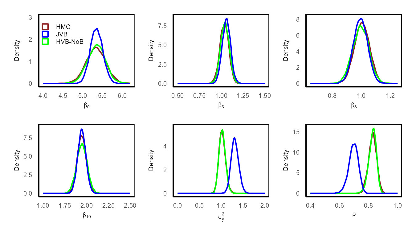
Refer to caption
Figure S1: Posterior densities of SEM parameters under MAR for the simulated dataset with n=625𝑛625n=625 and 25%percent2525\% missing values (nu=156subscript𝑛𝑢156n_{u}=156) estimated using the HMC, JVB and HVB-NoB methods
Refer to caption
(a) Posterior means
Refer to caption
(b) Posterior standard deviations
Figure S2: Comparison of the posterior means and standard deviation of missing values obtained using the JVB and HVB-NoB methods to those obtained using the HMC method for SEM under MAR with n=625𝑛625n=625 and 25%percent2525\% missing values (nu=156subscript𝑛𝑢156n_{u}=156)
n𝑛n n=625𝑛625n=625 n=1024𝑛1024n=1024 n=2500𝑛2500n=2500
missing percentage 25%percent2525\% 50%percent5050\% 75%percent7575\% 25%percent2525\% 50%percent5050\% 75%percent7575\% 25%percent2525\% 50%percent5050\% 75%percent7575\%
HMC 9.74 12.19 11.39 39.64 34.03 51.53 533.38 593.77 637.38
JVB 0.04 0.48 0.06 0.07 0.08 0.10 0.38 0.38 0.46
HVB- NoB 0.04 0.05 0.06 0.06 0.10 0.17 0.35 0.79 1.84
HVB- G - - - - 0.24 0.27 0.47 0.74 1.00
n𝑛n n=5,041𝑛5041n=5,041 n=7,569𝑛7569n=7,569 n=10,000𝑛10000n=10,000
missing percentage 25%percent2525\% 50%percent5050\% 75%percent7575\% 25%percent2525\% 50%percent5050\% 75%percent7575\% 25%percent2525\% 50%percent5050\% 75%percent7575\%
HMC - - - - - - - - -
JVB 1.285 1.610 2.066 3.519 4.18 5.09 7.95 7.93 10.46
HVB- NoB 1.63 6.49 16.39 4.49 26.61 72.13 10.44 69.92 201.14
HVB- G 1.69 2.66 3.20 4.04 5.77 6.38 9.06 10.88 12.59
Table S2: Average computing time (in seconds) of one iteration of the HMC, JVB, and HVB methods for estimating the SEM under MAR for different n𝑛n and different missing value (nusubscript𝑛𝑢n_{u}) percentages. For HVB-G, the tuning parameters, such as the block size (ksuperscript𝑘k^{*}) and the number of draws (N1subscript𝑁1N_{1}) of the Gibbs iteration scheme, are set to N1=5subscript𝑁15N_{1}=5 and k=500superscript𝑘500k^{*}=500, respectively. The HVB-G is not implemented for nu<1000subscript𝑛𝑢1000n_{u}<1000. The HMC is not implemented for n>5000𝑛5000n>5000

Table S2 displays the average computing time per iteration (in seconds) for the VB and HMC methods for different n𝑛n and nusubscript𝑛𝑢n_{u} under the MAR mechanism. The HVB-G method is not implemented when nusubscript𝑛𝑢n_{u} is relatively small (nu<1,000subscript𝑛𝑢1000n_{u}<1,000). The HMC method is computationally expensive when n𝑛n is large and is not implemented when n>5,000𝑛5000n>5,000. The HMC method is much more computationally expensive than the VB methods, regardless of the values of n𝑛n and nusubscript𝑛𝑢n_{u}. Although it cannot accurately capture the posterior distributions of the parameters σy2subscriptsuperscript𝜎2y\sigma^{2}_{\textbf{y}}, ρ𝜌\rho and the posterior standard deviation of the missing values (see Figures 1 and 2 of the main paper, and Figures S1 and S5 of the online supplement), the JVB method is generally the fastest among all the methods. For smaller values of n𝑛n and nusubscript𝑛𝑢n_{u}, the HVB-NoB algorithm is faster than the HVB-G method. The computing time of HVB-NoB increases rapidly as n𝑛n and nusubscript𝑛𝑢n_{u} increase, while HVB-G exhibits lower computing time than HVB-NoB, especially for high missing value percentages.

S4.2 Simulation study under MNAR

Under MNAR, with n=625𝑛625n=625 and 25%percent2525\% missing values percentage, the posterior distributions of the SEM and missing value model parameters obtained from the JVB algorithm and all three HVB algorithms are close to those obtained from the HMC method as shown in Figure S3. While the posterior means of missing values are nearly identical across HMC, JVB, and three HVB methods, the posterior standard deviations of missing values obtained using the JVB method are slightly different from those obtained from HMC, as shown in Figure S4.
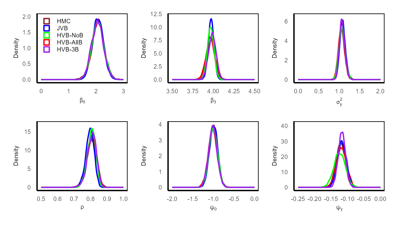
Refer to caption
Figure S3: Posterior densities of SEM and missing value model parameters obtained using the HMC, JVB, HVB-NoB, HVB-AllB, and HVB-3B methods, under MNAR with n=625𝑛625n=625 and nu=170subscript𝑛𝑢170n_{u}=170 (around 25%percent2525\% missing)
Refer to caption
(a) Posterior means
Refer to caption
(b) Posterior standard deviations
Figure S4: Comparison of the posterior means and standard deviations of missing values from JVB and HVBs compared to that of HMC under MNAR with n=625𝑛625n=625 and around 75%percent7575\% missing (nu=170subscript𝑛𝑢170n_{u}=170)

S5 Additional figures from simulation study section of the main paper

This section provides additional figures related to the simulation study presented in Section 4 of the main paper.

S5.1 Simulation study under MAR
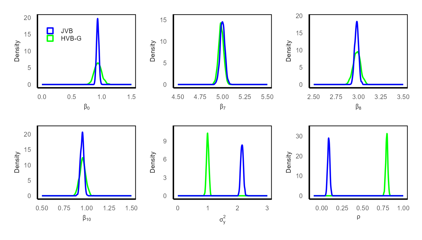
Refer to caption
Figure S5: Posterior densities of SEM parameters under MAR for the simulated data with n=10,000𝑛10000n=10,000 and 75%percent7575\% missing values (nu=7,500subscript𝑛𝑢7500n_{u}=7,500) estimated using the JVB and HVB-G methods
Refer to caption
Figure S6: Comparison of the posterior means of missing values estimated using the JVB and HVB-G methods with the true missing values under MAR for the simulated dataset with n=10,000𝑛10000n=10,000 and 75%percent7575\% missing values (nu=7,500subscript𝑛𝑢7500n_{u}=7,500)

In Figure S5, we compare the posterior densities of SEM parameters obtained using the JVB and HVB-G algorithms for n=10,000𝑛10000n=10,000 and nu=7,500subscript𝑛𝑢7500n_{u}=7,500 under MAR. The posterior distributions of ρ𝜌\rho and σy2subscriptsuperscript𝜎2y\sigma^{2}_{\textbf{y}} obtained from JVB are different from their true values. In contrast, the posterior means from HVB-G align with the true values for all parameters. Figure S6 compares the posterior means of the missing values estimated by the two VB methods with the true missing values. The posterior means of the missing values obtained from both methods are close to the true values.

S5.2 Simulation study under MNAR
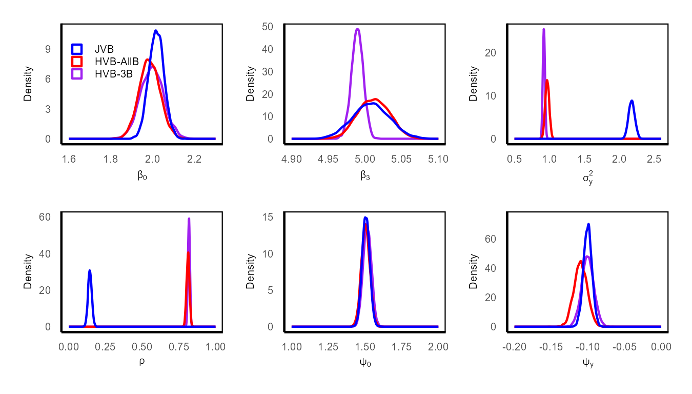
Refer to caption
Figure S7: Posterior densities of SEM and missing value model parameters under MNAR with n=10,000𝑛10000n=10,000 and nu=7,542subscript𝑛𝑢7542n_{u}=7,542 (around 75%percent7575\% missing) using the JVB and different HVB methods

In Figure S7, we compare the posterior densities of SEM and missing data model parameters obtained using the JVB, HVB-AllB, and HVB-NoB algorithms for n=10,000𝑛10000n=10,000 and nu=7,542subscript𝑛𝑢7542n_{u}=7,542 under MNAR. The posterior distributions obtained from the HVB-AllB and HVB-3B algorithms are almost identical, except for a slight difference in the posterior distribution of β0subscript𝛽0\beta_{0}. The posterior distributions of ρ𝜌\rho and σy2subscriptsuperscript𝜎2y\sigma^{2}_{\textbf{y}} obtained from JVB are significantly different from their true values. In contrast, the posterior means of all parameters from HVB-AllB and HVB-3B align with the true values.

Figure S8 compares the posterior means of the missing values estimated by the three VB methods with the true missing values. The posterior means of the missing values obtained from all methods are close to the true values. However, the posterior means of the missing values from the HVB-AllB and HVB-3B methods are closer to the true values, as they are more concentrated along the diagonal line compared to JVB.
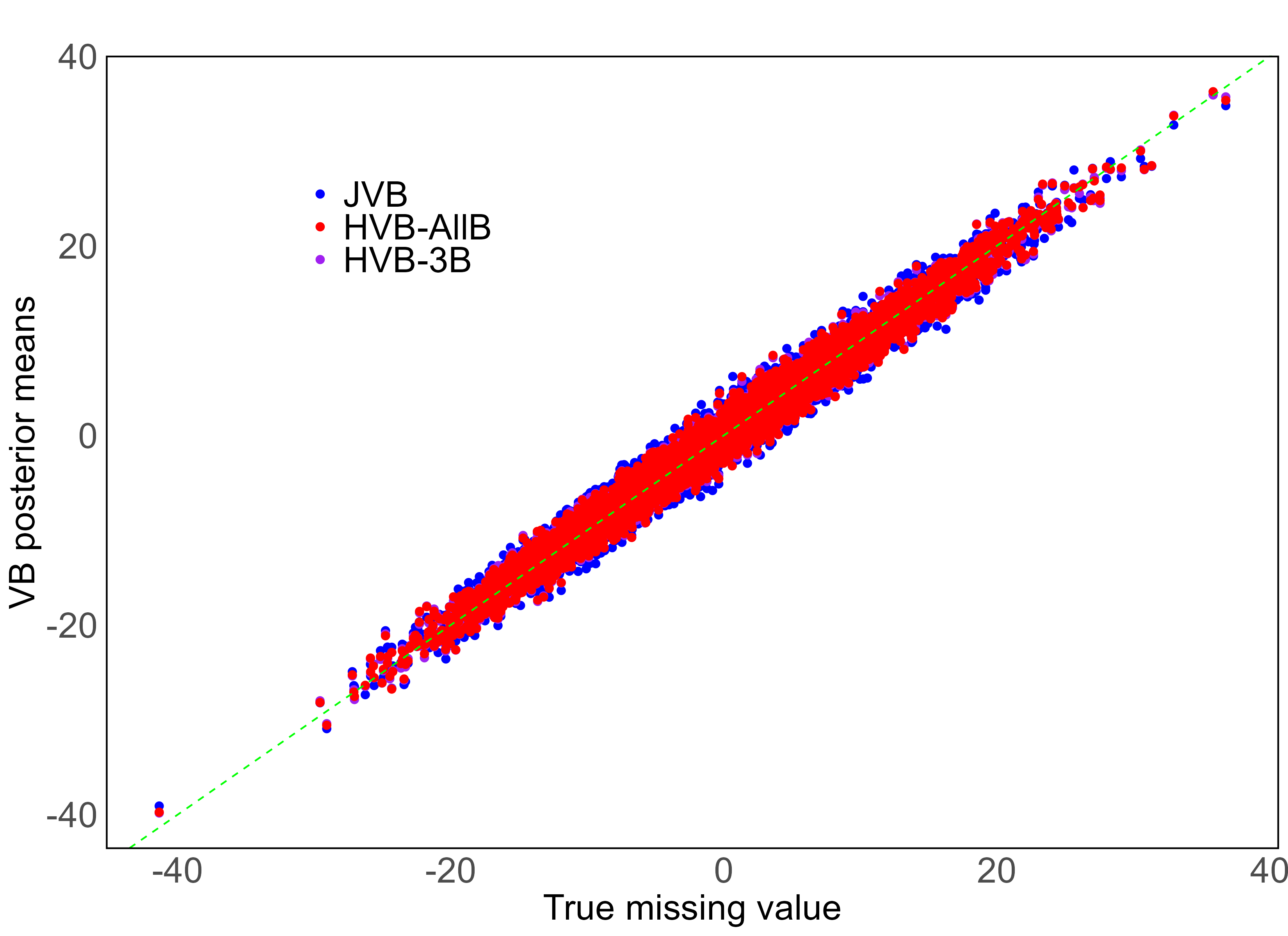
Refer to caption
Figure S8: Comparison of the posterior means of the missing values obtained from JVB, HVB-AllB, and HVB-3B with the true missing values under MNAR with n=7,542𝑛7542n=7,542, and nu=10,000subscript𝑛𝑢10000n_{u}=10,000 (around 75%percent7575\% missing)

S6 Additional figures and tables from real data section of the main paper

This section provides additional figures and tables related to the real data application presented in Section 5 of the main paper.

S6.1 SEM under MAR
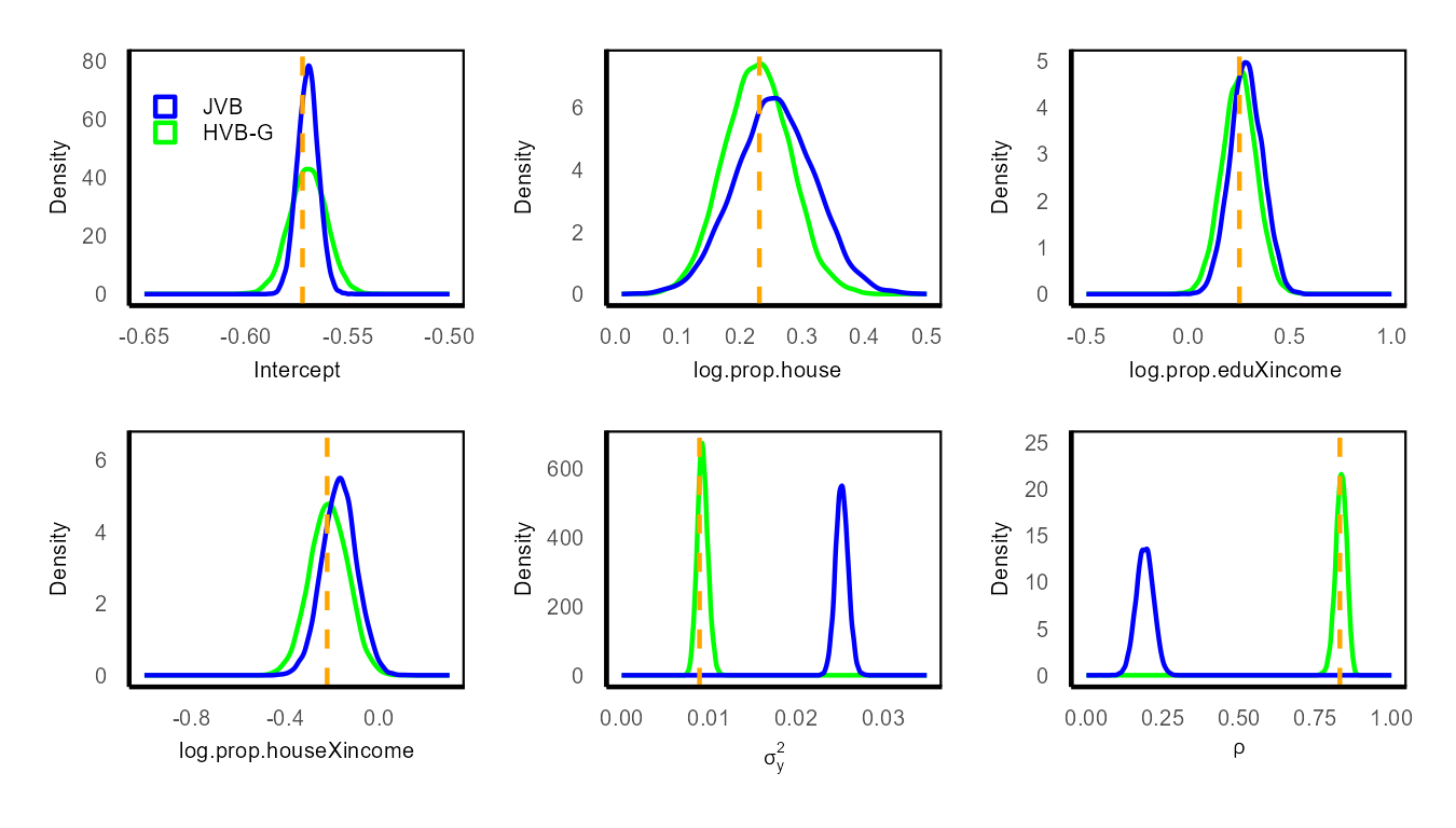
Refer to caption
Figure S9: Posterior densities of SEM parameters for 1980 presidential election dataset under MAR using JVB and HVB-G with 75%percent7575\% missing values (nu=2,330subscript𝑛𝑢2330n_{u}=2,330). The vertical lines indicate marginal ML estimates

Figure S9 presents the posterior densities of SEM parameters estimated using the JVB and HVB-G methods with 75%percent7575\% of missing responses (nu=2,330subscript𝑛𝑢2330n_{u}=2,330). The vertical lines indicate the marginal ML estimates. The figure shows that the JVB method yields different posterior density estimates for the parameters σy2subscriptsuperscript𝜎2y\sigma^{2}_{\textbf{y}} and ρ𝜌\rho compared to the HVB-G method. The posterior mean estimates obtained using the HVB-G algorithm are closer to the marginal ML estimates than those from the JVB method.
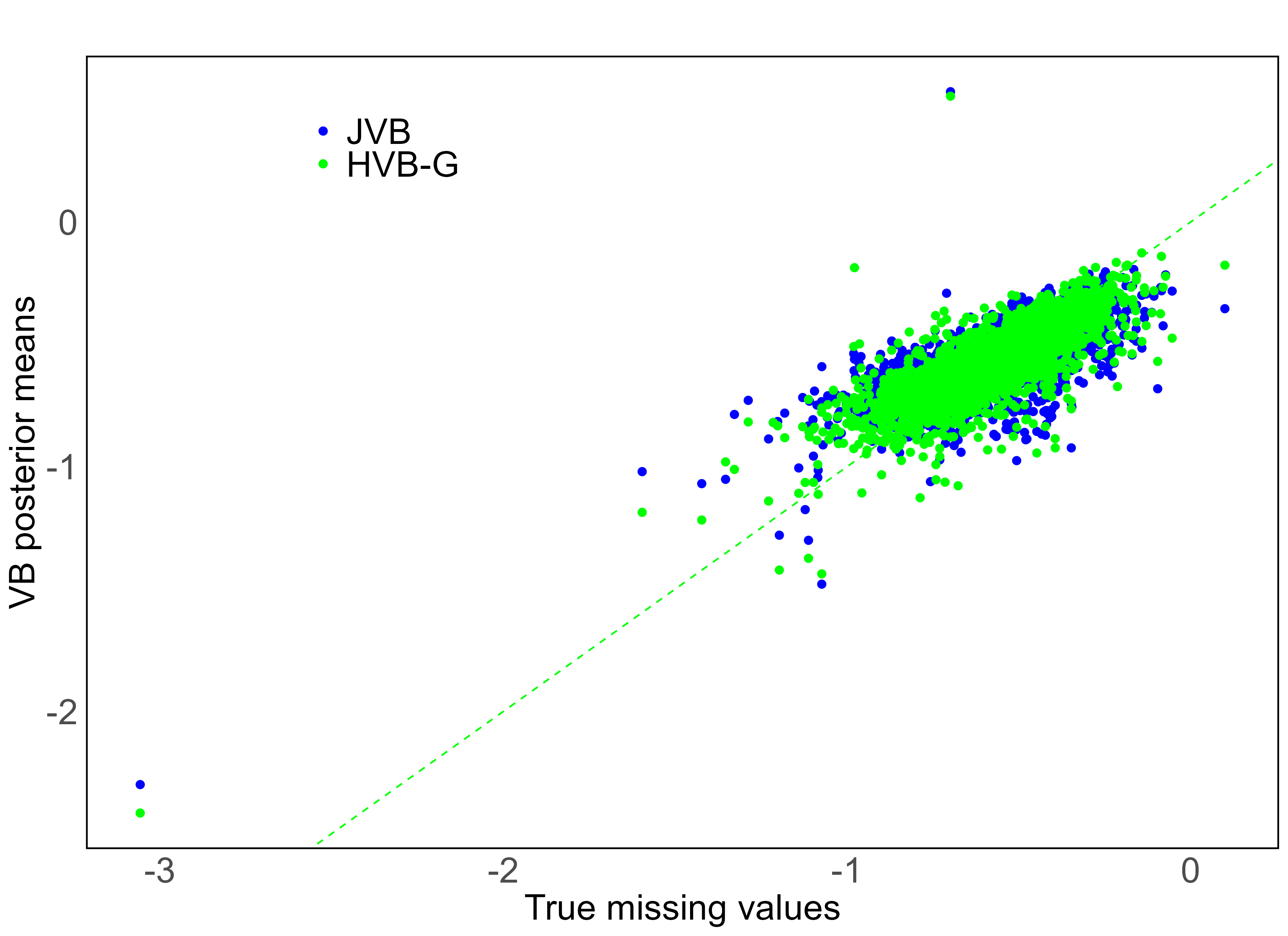
Refer to caption
Figure S10: Comparison of the posterior means of missing values obtained from the JVB and HVB-G algorithms with the true missing response values for the 1980 presidential election dataset under MAR with 75%percent7575\% missing values (nu=2,330subscript𝑛𝑢2330n_{u}=2,330)

Figure S10 compares the posterior means of missing values obtained from the JVB and HVB-G algorithms with the true missing values. The figure shows that the estimates of missing values from HVB-G are slightly closer to the true missing values than those obtained from the JVB algorithm, see also the MSE values in Table 6 of the main paper.

Table S3 presents the ML estimates with their standard errors and the posterior means with their standard deviations obtained from the JVB and HVB-G methods for SEM parameters for the 1980 presidential election dataset with 75% missing values under MAR. The posterior means and standard deviations obtained from HVB-G align more closely with the estimates from marginal ML than those from JVB.

Table S3: Marginal ML estimates (with standard errors in brackets), and posterior means (with posterior standard deviations in brackets) of SEM parameters estimated by the JVB and HVB-G algorithms for the 1980 presidential election dataset with 75%percent7575\% (nu=2,330subscript𝑛𝑢2330n_{u}=2,330) missing values under MAR
marginal ML JVB HVB-G
intercept(β0)𝑖𝑛𝑡𝑒𝑟𝑐𝑒𝑝𝑡subscript𝛽0intercept~{}(\beta_{0}) -0.5723 (0.01087) -0.5697 (0.0051) -0.5696 (0.0091)
log.prop.edu(β1)formulae-sequence𝑙𝑜𝑔𝑝𝑟𝑜𝑝𝑒𝑑𝑢subscript𝛽1log.prop.edu~{}(\beta_{1}) -0.1721 (0.1246) -0.0826 ( 0.0815) -0.1816 (0.0964)
log.prop.house(β2)formulae-sequence𝑙𝑜𝑔𝑝𝑟𝑜𝑝𝑜𝑢𝑠𝑒subscript𝛽2log.prop.house~{}(\beta_{2}) 0.2312 (0.0657) 0.2563 ( 0.0637) 0.2280 ( 0.0527)
income(β3)𝑖𝑛𝑐𝑜𝑚𝑒subscript𝛽3income~{}(\beta_{3}) -0.1233 (0.0847) -0.0946 (0.0525) -0.1234 (0.0669)
log.prop.edu×log.prop.house(β4)formulae-sequence𝑙𝑜𝑔𝑝𝑟𝑜𝑝𝑒𝑑𝑢𝑙𝑜𝑔𝑝𝑟𝑜𝑝𝑜𝑢𝑠𝑒subscript𝛽4log.prop.edu\times log.prop.house~{}(\beta_{4}) -0.1424 (0.1353) -0.0780 (0.0804) -0.1444 (0.1059)
log.prop.edu×income(β5)formulae-sequence𝑙𝑜𝑔𝑝𝑟𝑜𝑝𝑒𝑑𝑢𝑖𝑛𝑐𝑜𝑚𝑒subscript𝛽5log.prop.edu\times income~{}(\beta_{5}) 0.2521 (0.0970) 0.2870 (0.0797) 0.2517 ( 0.0843)
log.prop.house×income(β6)formulae-sequence𝑙𝑜𝑔𝑝𝑟𝑜𝑝𝑜𝑢𝑠𝑒𝑖𝑛𝑐𝑜𝑚𝑒subscript𝛽6log.prop.house\times income~{}(\beta_{6}) -0.2213 (0.1066) -0.1690 (0.0733) -0.2137 (0.0818)
log.prop.edu×log.prop.houseformulae-sequence𝑙𝑜𝑔𝑝𝑟𝑜𝑝𝑒𝑑𝑢𝑙𝑜𝑔𝑝𝑟𝑜𝑝𝑜𝑢𝑠𝑒log.prop.edu\times log.prop.house ×income(β7)absent𝑖𝑛𝑐𝑜𝑚𝑒subscript𝛽7\times income~{}(\beta_{7}) 0.2076 (0.1209) 0.2582 (0.0989) 0.2203 (0.1073)
σy2subscriptsuperscript𝜎2y\sigma^{2}_{\textbf{y}} 0.0089 (0.0006) 0.0253 (0.0007) 0.0093 (0.0006)
ρ𝜌\rho 0.8306 (0.0181) 0.1916 (0.0282) 0.8346 (0.0182)

S6.2 SEM under MNAR

Refer to caption
Figure S11: Posterior densities of SEM and missing value model parameters for the 1980 presidential election dataset under MNAR obtained using the JVB, HVB-AllB, and HVB-3B methods with approximately 80%percent8080\% missing values (nu=2,477subscript𝑛𝑢2477n_{u}=2,477)

Figure S11 compares the posterior densities of SEM and missing data model parameters obtained from the JVB, HVB-AllB, and HVB-3B methods for the 1980 presidential election dataset with around 80%percent8080\% missing values under MNAR. The figure shows that, except for σy2subscriptsuperscript𝜎2y\sigma^{2}_{\textbf{y}} and ρ𝜌\rho, the posterior densities of SEM and missing data model parameters obtained from different algorithms are almost identical. For σy2subscriptsuperscript𝜎2y\sigma^{2}_{\textbf{y}} and ρ𝜌\rho, the posterior densities obtained from HVB-AllB and HVB-3B differ from those obtained using JVB.
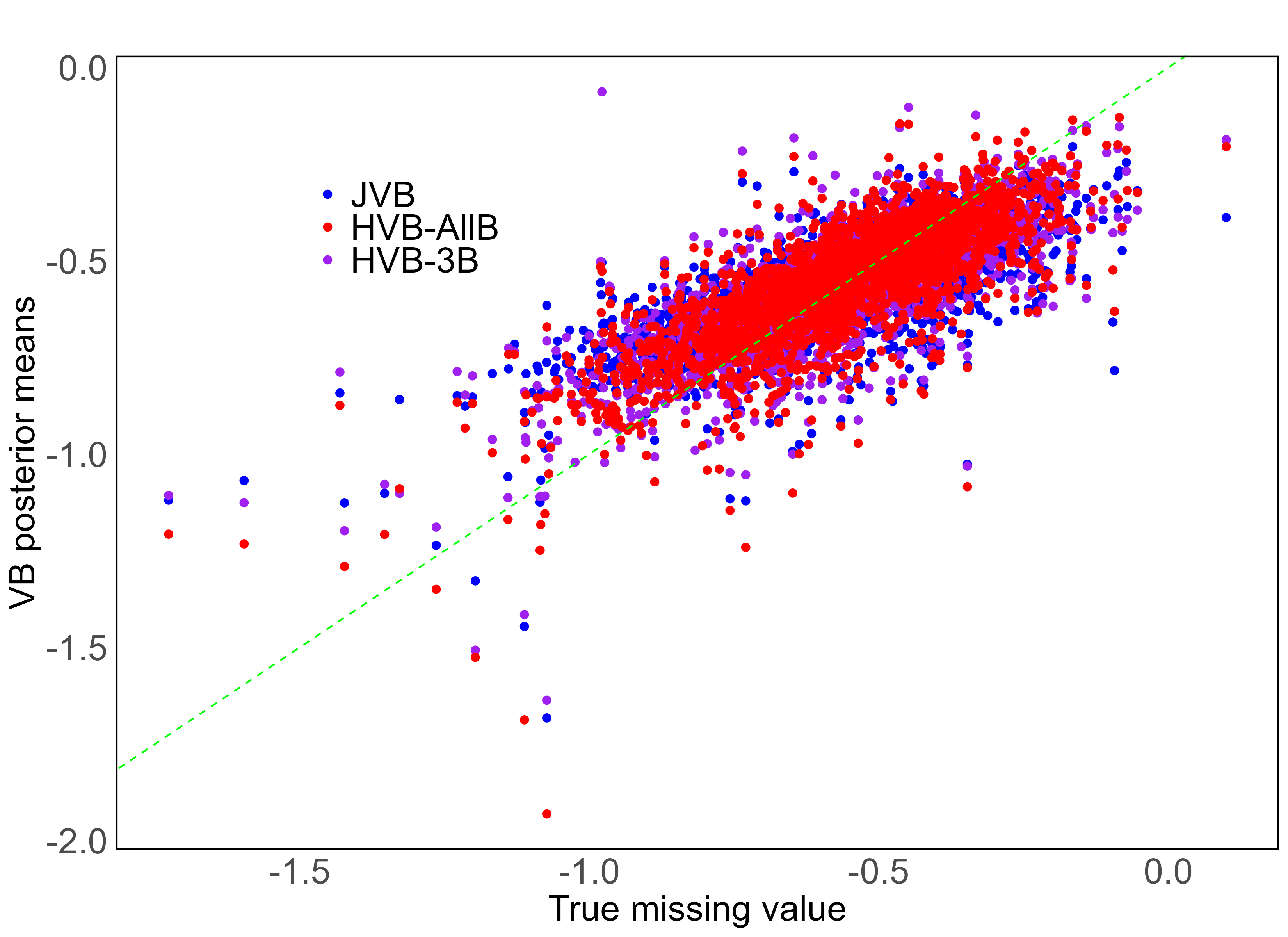
Refer to caption
Figure S12: Comparison of the posterior means of the missing values obtained from JVB, HVB-AllB, and HVB-3B with the true missing values for the 1980 presidential election dataset under MNAR with 80%percent8080\% missing values (nu=2,477subscript𝑛𝑢2477n_{u}=2,477)

Figure S12 compares the posterior means of missing values obtained from the JVB, HVB-AllB, and HVB-3B methods with the true missing values. The estimates from the HVB-AllB method are slightly closer to the true missing values than those from the HVB-3B and JVB methods.

Table S4 presents the posterior means and standard deviations of SEM and missing data model parameters obtained from the JVB, HVB-AllB, and HVB-3B algorithms, and the true values for missing data model parameters. The posterior means and standard deviations from the HVB-AllB and HVB-3B algorithms are very close. However, the estimates from the JVB algorithm differ, particularly for ρ𝜌\rho and σY2subscriptsuperscript𝜎2Y\sigma^{2}_{\textbf{Y}}.

Table S4: Posterior means (with posterior standard deviations inside brackets) of SEM and missing data model parameters, and the true parameter values for the missing data model parameters under MNAR obtained from the JVB, HVB-AllB, and HVB-3B methods for the 1980 presidential election datase with approximately 80%percent8080\% missing values (nu=2477subscript𝑛𝑢2477n_{u}=2477)
True value JVB HVB-AllB HVB-3B
intercept(β0)𝑖𝑛𝑡𝑒𝑟𝑐𝑒𝑝𝑡subscript𝛽0intercept~{}(\beta_{0}) NA -0.5815 (0.0112) -0.5773 (0.0163) -0.5689 (0.0078)
log.prop.edu(β1)formulae-sequence𝑙𝑜𝑔𝑝𝑟𝑜𝑝𝑒𝑑𝑢subscript𝛽1log.prop.edu~{}(\beta_{1}) NA 0.1345 (0.0851) 0.1078 (0.0975) 0.0913 (0.0539)
log.prop.house(β2)formulae-sequence𝑙𝑜𝑔𝑝𝑟𝑜𝑝𝑜𝑢𝑠𝑒subscript𝛽2log.prop.house~{}(\beta_{2}) NA 0.3732 (0.0583) 0.4094 (0.0665) 0.4139 (0.0398)
income(β3)𝑖𝑛𝑐𝑜𝑚𝑒subscript𝛽3income~{}(\beta_{3}) NA -0.2617 (0.0629) -0.2941 ( 0.0728) -0.2684 (0.0460)
log.prop.edu×log.prop.house(β4)formulae-sequence𝑙𝑜𝑔𝑝𝑟𝑜𝑝𝑒𝑑𝑢𝑙𝑜𝑔𝑝𝑟𝑜𝑝𝑜𝑢𝑠𝑒subscript𝛽4log.prop.edu\times log.prop.house~{}(\beta_{4}) NA 0.2177 (0.0905) 0.2362 (0.0953) 0.2108 ( 0.0738)
log.prop.edu×income(β5)formulae-sequence𝑙𝑜𝑔𝑝𝑟𝑜𝑝𝑒𝑑𝑢𝑖𝑛𝑐𝑜𝑚𝑒subscript𝛽5log.prop.edu\times income~{}(\beta_{5}) NA 0.0582 (0.0499) 0.0312 (0.0487) 0.0736 (0.0395)
log.prop.house×income(β6)formulae-sequence𝑙𝑜𝑔𝑝𝑟𝑜𝑝𝑜𝑢𝑠𝑒𝑖𝑛𝑐𝑜𝑚𝑒subscript𝛽6log.prop.house\times income~{}(\beta_{6}) NA -0.4237 (0.0918) -0.5056 (0.0956) -0.4701 (0.0556)
log.prop.edu×log.prop.houseformulae-sequence𝑙𝑜𝑔𝑝𝑟𝑜𝑝𝑒𝑑𝑢𝑙𝑜𝑔𝑝𝑟𝑜𝑝𝑜𝑢𝑠𝑒log.prop.edu\times log.prop.house ×income(β7)absent𝑖𝑛𝑐𝑜𝑚𝑒subscript𝛽7\times income~{}(\beta_{7}) NA -0.0607 (0.0605) -0.1038 (0.0659) -0.0848 (0.0457)
σy2subscriptsuperscript𝜎2y\sigma^{2}_{\textbf{y}} NA 0.0242 (0.0006) 0.0109 (0.0008) 0.0154 (0.0006)
ρ𝜌\rho NA 0.1634 (0.0259) 0.8004 (0.0171) 0.6990 (0.0186)
ψ0subscript𝜓0\psi_{0} 1.4 1.6622 (0.1977) 1.6504 (0.1934) 1.5891 (0.1455)
ψxsubscript𝜓superscriptx\psi_{\textbf{x}^{*}} 0.5 0.5227 (0.0519) 0.5172 (0.0497) 0.5376 (0.0454)
ψysubscript𝜓y\psi_{\textbf{y}} -0.1 0.3540 (0.3252) 0.3316 (0.3269) 0.2286 (0.2354)

S7 Convergence analysis of the VB methods

To evaluate the convergence of the proposed JVB method, we plot the lower bound over iterations. For the HVB algorithms, we analyse trajectories of variational means of the parameters across iterations for the simulation study and the real application.

S7.1 Convergence Analysis for the Simulation Studies

This subsection provides convergence analysis plots for the simulation studies presented in Section 4 of the main paper, as well as in Section S4 of the online supplement. Generally, HVB algorithms converge more rapidly compared to JVB algorithms.

S7.1.1 Convergence analysis for the simulation studies for the SEM under MAR

Figures S13, S15, and S17 illustrate lower bounds for the JVB algorithm (the left figure), and the trajectories of variational means of SEM parameters for the HVB algorithm (the right figure) across VB iterations, under MAR, for different values of n𝑛n and nusubscript𝑛𝑢n_{u}. All VB algorithms achieve convergence well before the final iteration. The HVB algorithms consistently reach convergence in fewer iterations than the JVB algorithm.

Figures S14 and S16 display trace plots of posterior samples for SEM parameters under the MAR mechanism, obtained using the HMC method after discarding burn-in iterations for the simulated datasets with n=625𝑛625n=625 and different missing value percentages (nusubscript𝑛𝑢n_{u}). The trace plots indicate good mixing for both cases.
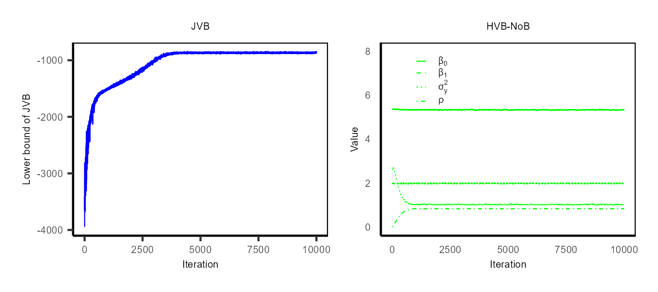
Refer to caption
Figure S13: The lower bound for the JVB algorithm (left figure), and the trajectories of variational means of SEM parameters for the HVB-NoB algorithm over iterations (right figure), under MAR for the simulated dataset with n=625𝑛625n=625 and nusubscript𝑛𝑢n_{u}= 156 (i.e. missing percentage is 25%)
Refer to caption
Figure S14: Trace plots of SEM posterior samples of SEM parameters under MAR from the HMC method after excluding burn-in iterations for the simulated dataset with n=625𝑛625n=625 and nu=156subscript𝑛𝑢156n_{u}=156 (i.e., the missing percentage is 25%)
Refer to caption
Figure S15: The lower bound for the JVB algorithm (left figure), and the trajectories of variational means of SEM parameters for the HVB-NoB algorithm over iterations (right figure), under MAR for the simulated dataset with n=625𝑛625n=625, nusubscript𝑛𝑢n_{u}= 469 (i.e. missing percentage is 75%)
Refer to caption
Figure S16: Trace plots of posterior samples of SEM parameters under MAR from the HMC method after excluding burn-in iterations for the simulated dataset with n=625𝑛625n=625 and nu=469subscript𝑛𝑢469n_{u}=469 (i.e., the missing percentage is 75%)
Refer to caption
Figure S17: The lower bound for the JVB algorithm (left figure), and the trajectories of variational means of SEM parameters for the HVB-G algorithm over iterations (right figure), under MAR for the simulated dataset with n=10,000𝑛10000n=10,000, nu=7,500subscript𝑛𝑢7500n_{u}=7,500 (i.e. missing percentage is 75%)

S7.1.2 Convergence analysis for the simulation studies for the SEM under MNAR

Figures S18, S20, and S22 show lower bounds for the JVB algorithm (displayed in the top left subplot), and the trajectories of variational means of SEM and missing data model parameters for the HVB algorithms (shown in the remaining subplots) across VB iterations, under MNAR, for the simulated datasets with various combinations of n𝑛n and nusubscript𝑛𝑢n_{u}. As observed in the simulation study under MAR, all VB algorithms achieve convergence well before the final iteration. Additionally, the HVB algorithms consistently achieve convergence in fewer iterations compared to the JVB algorithm.

Figures S19 and S21 present trace plots of posterior samples of SEM parameters under the MNAR mechanism, obtained using the HMC method after discarding burn-in iterations, for the simulated datasets with a sample size of n=625𝑛625n=625 and different missing value percentages (nusubscript𝑛𝑢n_{u}). These trace plots display stable, random-like patterns, suggesting good mixing for all SEM parameters.
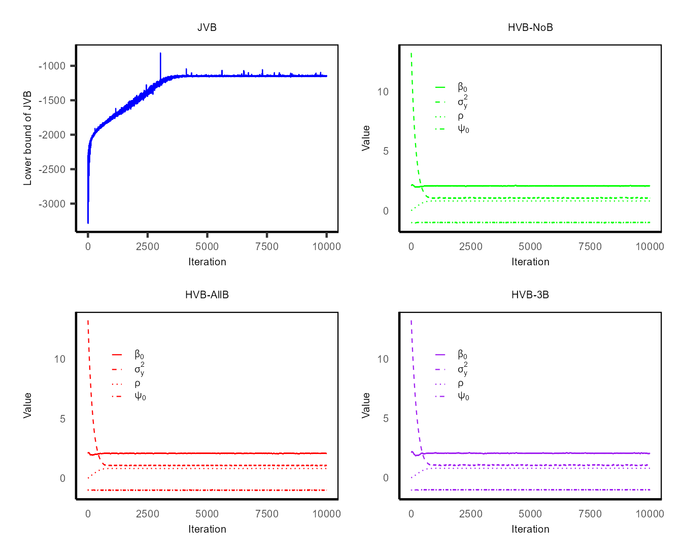
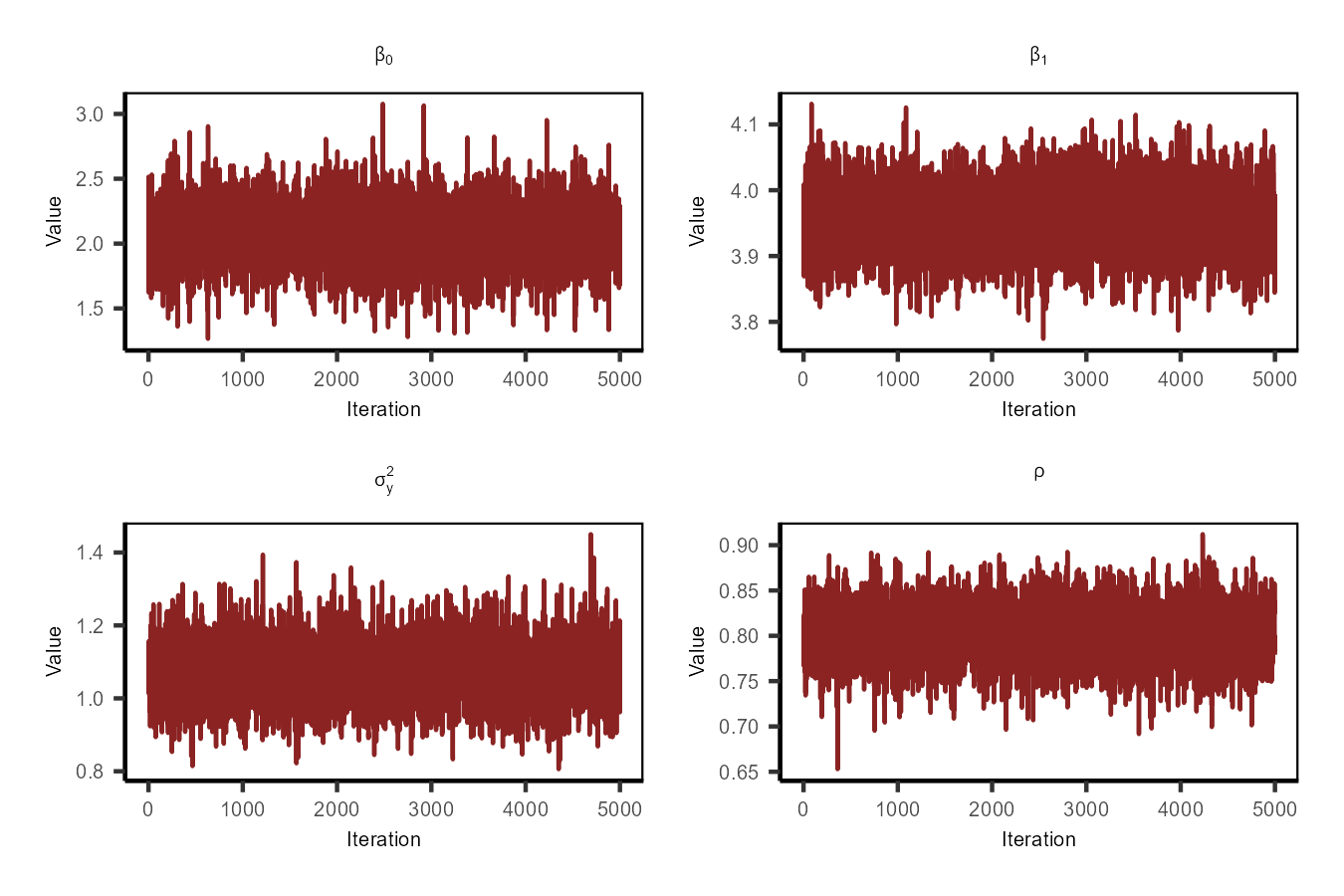
Refer to caption
Figure S18: The lower bound for the JVB algorithm (top left figure), and the trajectories of variational means of SEM and missing data model parameters for the HVB algorithms over iterations (top right figure and bottom figures), under MNAR for the simulated dataset with n=625𝑛625n=625, nusubscript𝑛𝑢n_{u}= 170 (i.e. missing percentage is 25%)
Refer to caption
Figure S19: Trace plots of posterior samples of SEM parameters under MNAR from the HMC method after excluding burn-in iterations for the simulated dataset with n=625𝑛625n=625 and nu=170subscript𝑛𝑢170n_{u}=170 (i.e., the missing percentage is 25%)
Refer to caption
Figure S20: The lower bound for the JVB algorithm (top left figure), and the trajectories of variational means of SEM and missing data model parameters for the HVB algorithms over iterations (top right figure and bottom figures), under MNAR for the simulated dataset with n=625𝑛625n=625, nusubscript𝑛𝑢n_{u}= 469 (i.e. missing percentage is 75%)
Refer to caption
Figure S21: Trace plots of posterior samples of SEM parameters unde MNAR from the HMC method after excluding burn-in iterations for the simulated dataset with n=625𝑛625n=625 and nu=469subscript𝑛𝑢469n_{u}=469 (i.e., the missing percentage is 75%)
Refer to caption
Figure S22: The lower bound for the JVB algorithm (top left figure), and the trajectories of variational means of SEM and missing data model parameters for the HVB algorithms over iterations (top right and bottom left figures), under MNAR for the simulated dataset with n=10,000𝑛10000n=10,000, nu=7,542subscript𝑛𝑢7542n_{u}=7,542 (i.e. missing percentage is approximately 75%)

S7.2 Convergence analysis for the Real data examples

This subsection provides convergence analysis plots for the real world example presented in Section 5 of the main paper.

S7.2.1 Convergence analysis for Real data examples under MAR

Figure S23 shows the lower bound for the JVB algorithm, and the trajectories of variational means of SEM parameters obtained using the HVB-G algorithm across iterations, for the 1980 presidential election dataset, under MAR with nu=2,330subscript𝑛𝑢2330n_{u}=2,330. These plots clearly indicate convergence for both the HVB-G and JVB algorithms.
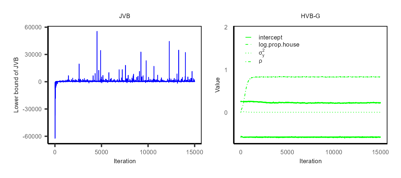
Refer to caption
Figure S23: The lower bound for the JVB algorithm (left figure), and the trajectories of variational means of SEM parameters for the HVB-G algorithm over iterations (right figure) for the 1980 presidential election dataset, under MAR with nu=2,330subscript𝑛𝑢2330n_{u}=2,330 (i.e. missing percentage is 75%percent7575\%)

S7.2.2 Convergence analysis for the Real data example under MNAR

Figure S24 illustrates the lower bound for the JVB algorithm, and the trajectories of the variational means of SEM and missing data model parameters for the HVB algorithms; HVB-AllB and HVB-3B, across iterations for the 1980 presidential election dataset under MNAR with nu=2,477subscript𝑛𝑢2477n_{u}=2,477. Flat lines indicate that all algorithms have converged before the 15,000th15superscript000𝑡15,000^{th} iteration.

Refer to caption
Figure S24: The lower bound for the JVB algorithm (top left figure), and the trajectories of variational means of SEM and missing data model parameters for the HVB-AllB and HVB-3B algorithms over iterations (top right and bottom left figures) for the 1980 presidential election dataset, under MNAR with nu=2,477subscript𝑛𝑢2477n_{u}=2,477 (i.e. missing percentage is around 80%percent8080\%)