FakeInversion: Learning to Detect Images from Unseen
Text-to-Image Models by Inverting Stable Diffusion

Abstract

Due to the high potential for abuse of GenAI systems, the task of detecting synthetic images has recently become of great interest to the research community. Unfortunately, existing image-space detectors quickly become obsolete as new high-fidelity text-to-image models are developed at blinding speed. In this work, we propose a new synthetic image detector that uses features obtained by inverting an open-source pre-trained Stable Diffusion model. We show that these inversion features enable our detector to generalize well to unseen generators of high visual fidelity (e.g., DALL·E 3) even when the detector is trained only on lower fidelity fake images generated via Stable Diffusion. This detector achieves new state-of-the-art across multiple training and evaluation setups. Moreover, we introduce a new challenging evaluation protocol that uses reverse image search to mitigate stylistic and thematic biases in the detector evaluation. We show that the resulting evaluation scores align well with detectors’ in-the-wild performance, and release these datasets as public benchmarks for future research.

Figure 1: (left) We propose a new synthetic image detectorwhitenew synthetic image detector that uses two additional input signals derived from a fixed pre-trained Stable Diffusion [45]: an inverted latent noise map and the reconstructed input image. (middle) Our detector is trained using fake images generated using Stable Diffusion and real LAION images. It achieves state-of-the-art generalization performancewhitestate-of-the-art generalization performance in detecting unseen text-to-image generators. (right) To ensure that the performance evaluation does not favor detectors that are biased towards particular themes or styles, we introduce a new thematically and stylistically aligned evaluation benchmarkwhitenew thematically and stylistically aligned evaluation benchmark – we measure detector’s ability to discriminate fake images (e.g. DALL·E 3, Imagen) from real images with matching content and style found on the Internet using reverse image search (RIS).

1 Introduction

Recent advances in text-to-image modeling have made it easier than ever to generate harmful or misrepresentative content at scale. Moreover, new versions of most photorealistic commercial models are being continuously updated and released behind closed APIs, making it harder to keep fake image detectors up to date. In this work, we make significant strides towards building a GenAI detector that can reliably identify images from unseen photorealistic text-to-image models. Specifically, we propose a model that can be trained using fake images only from Stable Diffusion (SD) [45] and reliably detect images generated by recent open (Kandinsky [51], Wüerstchen [39], PixArt-$\alpha$ [16], etc.) and closed-source text-to-image models (Imagen [46], Midjourney [2], DALL·E 3 [12], etc.) of significantly higher visual fidelity.

Existing methods [17, 54, 37] focus primarily on detecting traces left by convolutional generators in a way that is robust to re-compression, resizing and other in-the-wild transformations. While these methods worked well for GANs and early diffusion models, we show that they, unfortunately, fail to generalize well to current photorealistic generative models, even when re-trained using better data. Recent diffusion detectors that rely on CLIP embeddings [37] or inversions [55] fail to generalize to challenging benchmarks. Drawing inspiration from recent works that showed that GANs tend to “omit hard objects” [11] and that text-to-image models lean towards “easily captionable” images [50], in this paper, we focus on detecting fake images by analyzing internal representations of an existing off-the-shelf text-to-image model.

In this paper, we introduce a new synthetic imagewhitesynthetic image detection methodwhitedetection method: FakeInversion. Our method uses features extracted from a lower-fidelity open-source text-to-image model (Stable Diffusion [45]) to detect images generated by unseen text-to-image generators. Specifically, our model takes as input 1) the original image, 2) the approximate noise map recovered via text-conditioned DDIM [52] inversion with Stable Diffusion (SD), and 3) the reconstruction obtained by “denoising” the approximate noise map (Figure 1). We show that these additional signals significantly improve the performance of the resulting detector on unseen new proprietary and open-source photorealistic text-to-image models, attaining a new state-of-the-art. We also provide an intuitive justification for why a diffusion detector needs such features to generalize well to unseen diffusion generators.

To deploy a synthetic image detector at scale, we need to make sure that it is not relying on content signals such as the presence of specific objects or styles in the image. If left unmitigated, such bias towards particular themes or styles would disproportionately marginalize particular groups when applied to detecting healthcare misinfo [1] or forged art [3] at scale. Unfortunately, existing evaluation protocols that measure a detector’s ability to differentiate between real and fake images drawn from very visually and thematically different distributions can not be used to test for the presence of such bias in the detector. For example, evaluating a fake detector using real COCO [33] images and fake images generated by DALL·E 3 [12] could favour a detector that assigns higher fakeness score to digital art, since COCO contains mostly natural images. To circumvent these issues, we propose a new evaluation protocolwhitenew evaluation protocol: SynRIS. For each set of synthetic images, we evaluate a given detector against a set of real images obtained by applying reverse image search (Figure 1) to given fake images – the resulting evaluation does not favor models biased towards any particular topic, theme, or style. We show that the proposed evaluation protocol is more reliable at evaluating the quality of the synthetic image detector, especially when applied to closed-source text-to-image models. We will release our evaluation benchmark (including datasets) for future research.

To summarize our contributions: 1) we introduce a new synthetic image detector that uses text-conditioned inversion maps extracted from Stable Diffusion; 2) we show that this additional feature improves the detector’s ability to detect images generated by unseen text-to-image models, achieving new state-of-the-art; 3) we propose a new challenging evaluation protocol that uses reverse image search to ensure that the classifier is not biased towards any particular theme or style; 4) we verify that this evaluation protocol reliably measures detector generalization to closed text-to-image models; and 5) we release our challenging benchmark for future research.

2 Related Work

In this section we first give a brief overview of the state-of-art in image-space detectors, then we discuss how recent works attempt to detect semantic inconsistencies in generated images, and finally discuss how our evaluation protocol compares to evaluation protocols used in prior work.

Artifact Detectors. Wang et al. [54] were among the first to show that a CNN detector (CNNDet) generalized well from more powerful GANs (e.g. ProGAN) to less powerful ones. Soon after, Chai et al. [14] extended this idea with a fully-convolutional network that classified individual image patches, Ju et al. [27] explored fusing global and local image features, Corvi et al. [17] explored better augmentation and downsampling strategies, Zhang et al. [61] and Frank et al. [20] explored artifacts in the spectrum of GAN-generated images, and Marra et al. [35] explored GAN fingerprinting.

Generation Inconsistencies. Several works have focused on understanding the semantic properties of generated images. For example, Bau et al. [11] showed that GANs avoid generating “hard objects” such as mirrors and TVs – that both humans and discriminators fail to notice missing. Recently, Ojha et al. [37] showed that image CLIP [42] embeddings are highly predictive of whether an image is fake, and Sha et al. [50] showed that images generated using text-to-image models tend to have higher CLIP similarity to their automatically inferred captions, suggesting that images generated by text-to-image models can often be described more fully by short text captions compared to images naturally occurring on the web. Inspired by these works, we also focus on properties of images beyond their low-level convolutional traces by examining internal representations of diffusion models obtained using DDIM inversion [52]. A concurrent work [55] found that DDIM image reconstruction residuals are predictive of whether an image is fake. In this paper we justify why image-space residuals are insufficient, and empirically verify that a detector that uses internal representations of a diffusion model generalizes better. We evaluate our model against the official DIRE checkpoint and perform an ablation using only reconstruction residuals.

Evaluation Protocols. Given that internal representations of diffusion models lack the low-level features necessary to perform generator trace detection, we need a way to ensure that the learned classifier does not overfit to particular objects or styles. Unfortunately, prior works focus either on open-source models with known training sets but lower visual fidelity or use dataset pairs of real and in-the-wild fake images that are too different both in style and content to ensure the lack of such bias. For example, recent works of Corvi et al. [17] and Ojha et al. [37] measure detectors’ ability to discriminate between DALL·E 2 images and a mix of Imagenet, COCO and UCID [48] or LAION respectively, and DIRE [55] focuses only on open-source lower fidelity generators such as SD and older generators trained on ImageNet and LSUN-Bedrooms [59]. In a concurrent work, Epstein et al. [19] evaluate how adding training data from older models affects the performance of the classifier on newer fakes, which is an important problem but different from the one we address in this paper.

To summarize, we are the first to show that text-conditioned DDIM inversion feature maps extracted from one diffusion model improve the ability of a detector to identify images generated by other higher-fidelity diffusion models. Moreover, we are the first to propose an evaluation procedure for GenAI detectors that ensures that the learned detector is not biased towards any style or theme, and to quantitatively verify that the resulting evaluation is more reliable.

3 Method

In this section, we first provide a background on diffusion models and DDIM inversion. Then, we introduce our detection method that makes use of text-conditioned DDIM inversion and give an intuitive justification for why having this signal is helpful for generalization.

Latent Diffusion Models. LDMs [45] first map high-resolution (in our case, 512$\times$512$\times$3) RGB images $x$ into low-resolution (64$\times$64$\times$4) latent images $z$ using a pre-trained encoder $E:\mathcal{X}\to\mathcal{Z}$. The original image can be recovered almost perfectly via a pre-trained decoder $D:\mathcal{Z}\to\mathcal{X}$. In the derivation below $z_{*}$ correspond to such latent images, rather than RGB images.

Conditional Diffusion Models and DDIM Inversion. To generate a new latent image $z$ conditioned on some vector $c$, a conditional denoising diffusion model [25] starts from a random noise map $z_{T}$ of the same shape and iteratively stochastically denoises it using a learned denoising network $\epsilon_{\theta}$ for a fixed number of steps, until a clean latent image $z_{0}$ is obtained. The process of sampling from a pre-trained diffusion model can be discretized into fewer steps and made deterministic through the use of DDIM sampling [52]. Notably, this sampling procedure enables “inverting” a clean image $z_{0}$ into a corresponding noise map $z_{T}$, such that when $z_{T}$ is denoised via DDIM sampling, we obtain a new latent $\hat{z}_{0}$ that is very close to the original $z_{0}$. Formally, to invert an image $z_{0}$, i.e., to obtain a corresponding noise map $z_{T}$, we iteratively add noise to its current estimate $z_{t}$ via the following conditional forward process starting from a clean latent image $z_{0}$:

$$z_{t+1}=\sqrt{\bar{\alpha}_{t+1}}f_{\theta}(z_{t},t,c)+\sqrt{1-\bar{\alpha}_{t+1}}\epsilon_{\theta}(z_{t},t,c)$$ (1)

where $z_{t}$ is the noisy latent at time $t$, vector $c$ is the conditioner, value $\bar{\alpha}$ is the DDIM noise scaling factor [52], noise $\epsilon_{\theta}(z_{t},t,c)$ is the prediction of the learned denoising function $\epsilon_{\theta}$ at time $t$, and $f_{\theta}(z_{t},t,c)$ is the best current estimate of the clean latent $z_{0}$:

$$f_{\theta}(z_{t},t,c)=\frac{z_{t}-\sqrt{1-\bar{\alpha}_{t}}\epsilon_{\theta}(z_{t},t,c)}{\sqrt{\bar{\alpha}_{t}}}$$ (2)

A imperfect reconstruction $\hat{z}_{0}$ can then be obtained via the deterministic conditional reverse process starting from $z_{T}$:

$$\hat{z}_{t-1}=\sqrt{\bar{\alpha}_{t-1}}f_{\theta}(\hat{z}_{t},t,c)+\sqrt{1-\bar{\alpha}_{t-1}}\epsilon_{\theta}(\hat{z}_{t},t,c).$$ (3)

We will refer to such full forward and reverse mapping as:

$$\hat{z}_{T}=F_{\theta}(z_{0},c),\quad\hat{z}_{0}=R_{\theta}(\hat{z}_{T},c).$$ (4)

Text Conditioning. In our case, the conditioning vector $c$ used to modulate the forward and reverse sampling processes is the embedding of the text prompt describing an image. In this work, we use an off-the-shelf captioner (BLIP 2 [32]) to obtain a text prompt describing an input image, and CLIP [42] to embed this text. Prior work showed that the realism of generated images can be improved through the use of classifier-free guidance [24]. Later, Mokady et al. [36] showed that classifier-free guidance leads to instability in DDIM inversion and proposed a mitigation strategy through fine-tuning parts of the model. Since we cannot afford fine-tuning on each incoming image, in this paper we do not use classifier-free guidance during inversion and sampling and use the original conditional update rules described above.

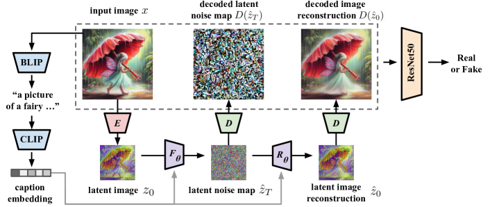
Figure 2: Proposed method. In addition to the original image itself ($x$), we also train our detector using the (decoded) noise map $D(\hat{z}_{T})$ and reconstruction $D(\hat{z}_{0})$ obtained by inverting the image through Stable Diffusion using DDIM. The original image is first mapped to the latent space with Stable Diffusion’s VAE Encoder. The latent image is then inverted and reconstructed through Stable Diffusion’s U-Net using DDIM while conditioned on the CLIP embedding of the image’s predicted BLIP caption. The latent noise map and reconstruction are mapped back to image space using Stable Diffusion’s VAE Decoder. The original image, decoded noise map, and decoded reconstruction are then concatenated and used as input for our ResNet Classifier.

GenAI Detector. As shown in Figure 2, given an input image $x$, we first caption that image using BLIP [32] and embed that caption into a vector $c$ using CLIP [42]. Then we compute the corresponding latent image $z_{0}=E(x)$ using a pre-trained encoder and obtain a latent DDIM noise map $\hat{z}_{T}$ using text-conditioned DDIM inversion with a pre-trained diffusion model. Then, we obtain a reconstructed latent image $\hat{z}_{0}$ using text-conditioned DDIM sampling and decode both the latent noise map $\hat{z}_{T}$ and the reconstruction $\hat{z}_{0}$ to image space using the decoder $D$. Finally, we apply a learned mapping $h_{\phi}:\mathcal{X}^{3}\to\mathbb{R}$ to these “images” to get a prediction logit. We learn the parameters of this function $\phi$ via backpropagation of the binary cross-entropy loss $\ell(\hat{y},y)$ on the training set of known fake and real images $\{(x,y)\}$:

$$c=\operatorname{CLIP}(\operatorname{BLIP}(x))$$ (5)

$$\hat{z}_{T}=F_{\theta}(E(x),c),\quad\hat{z}_{0}=R_{\theta}(\hat{z}_{T},c)$$ (6)

$$\phi^{*}=\operatorname*{argmin}_{\phi}\mathbb{E}_{x,y}[\,\ell\left(h_{\phi}\left(x,D(\hat{z}_{T}),D(\hat{z}_{0})\right),y\right)]$$ (7)

Intuition. But why would a diffusion detector benefit from having access to DDIM inversion of an image if it already has access to the image itself? Recent works [34, 47] showed that DDIM can be viewed as a first-order discretization of a neural probability-flow ODE. The bijection between observations $z_{0}$ and noise maps $z_{t}$ induced by this ODE can be used to evaluate the likelihood of the data via the change of variable. If we view the forward DDIM mapping $F_{\theta}$ as an approximation of that true bijective mapping between the $z_{0}$ and $z_{T}$ that introduces a discretization error $\delta$ into the inverted noise maps $\hat{z}_{T}$, causing the resampled image $\hat{z}_{0}$ to deviate from the original image $z_{0}$, it can be shown (see Sec. B.1) that, in the first-order approximation, the log-likelihood of the data given that underlying model can be estimated from the input image $z_{0}$, its imperfect reconstruction $\hat{z}_{0}$, and the noise map $z_{T}$ alone:

$$\log p(z_{0})\propto\log p_{z}(z_{T})-\langle\delta,\hat{z}_{0}-z_{0}\rangle/\|\delta\|^{2}$$ (8)

Notably, the expression above does not explicitly depend on the parameters $\theta$ other than through these three signals. Given that, under model misspecification, likelihood-based models tend to overgeneralize [26], producing samples that are unlikely under the true data distributions, and assuming that the class of diffusion-based models is similar enough to overgeneralize in similar ways, we propose that a model that has access to all signals required to internally perform some form of likelihood testing on input data against a particular text-to-image model (the image, its imperfect reconstruction, and the intermediate noise map) would generalize better to detect images generated via other diffusion models. Text conditioning $c$ further amplifies differences between log-likelihoods of distributions of fake and real images, making the corresponding test more powerful and consequently making inversions even more useful for detecting fake images. To sum up, GenAI detectors find discrepancies between the real data distribution and the approximation learned by the GenAI model. The equation above shows that proposed features enable a detector to get a rough estimate of whether a given image is of high probability under the approximate distribution learned by Stable Diffusion. We empirically verify that this “SD-likelihood” signal helps in detecting other generators.

4 Experiments

In this section, we discuss our training and evaluation sets, which baseline methods we use to compare, and the details of how we train our classifier.

Baselines. We compare our model to a representative set of the most recent state-of-art baselines (all published in 2023white2023) that open-sourced their training or inference code. DMDetwhiteDMDet [17] is a state-of-art RGB-only method that achieved significant generalization performance through the use of augmentations and a modified down-sampling strategy; authors released only the inference checkpoint. UFDwhiteUFD [37] is another recent state-of-the-art method that trains a linear classification head on top of the CLIP [42] embeddings of real and fake images. We use the official checkpoint and also retrain it from scratch on each of our training sets using the official code. DIREwhiteDIRE [55] is a concurrent work that showed that using image-space DDIM reconstruction residuals helps detection. The official checkpoint open-sourced by the authors has an issue causing its performance to be much lower than the performance reported in the paper; we discuss this in more detail in Sec. E.1. We also provide an ablation of our method that uses only DDIM residuals. This serves as a close approximation of what a DIRE-like method could achieve. We also include an older convolutional baseline CNNDetwhiteCNNDet [54] using its official checkpoint and code to retrain on our data.

Dataset	Data Size	Real Data	Real/Fake Source
DALL·E 2 [44]	700/700	RIS (ours)	fakes from [17]
DALL·E 3 [12]	3.3k/3.3k	RIS (ours)	fakes from [8]
Midjourney [2]	4.4k/4.4k	RIS (ours)	fakes from [9]
Imagen [46]	700/700	RIS (ours)	our fakes (see App. A)
Open-Source1	3.5k/3.5k (x11)	RIS (ours)	our fakes (see App. A)
DALL·E 2 (A)	1k/5k	Imagenet, COCO, UCID [48]	both reals/fakes from [17]
Craiyon (A)	1k/1k	LAION	both from [37]
LDM (A)	1k/1k	LAION	both from [37]

Table 1: Evaluation Datasets. We evaluate using 15 new RIS-based evaluation benchmarks (SynRIS (ours) – top) as well as existing academic (A) text-to-image evaluation dataset (bottom).

Eval Data		Training Data		FID	KID $\times 10^{-2}$
Fake	Real	ProGAN+LSUN	SD+LAION
DALL·E 2	LAION	0.233	0.043	163.5	2.7
	RIS (ours)	0.457	0.406	88.5	0.3
DALL·E 3	LAION	0.794	0.360	126.1	2.6
	RIS (ours)	0.920	0.795	93.6	0.4
Imagen	LAION	0.406	0.360	127.1	2.1
	WebLI	0.559	0.664	101.9	1.2
	RIS (ours)	0.620	0.720	83.6	0.2
Kandinsky 2	LAION	0.655	0.189	118.0	2.1
	RIS (ours)	0.857	0.686	88.9	0.4
SDXL	LAION	0.689	0.106	108.7	1.6
	RIS (ours)	0.874	0.551	93.0	0.4

Table 2: Difficulty of RIS vs LAION eval. FPR@0.8 recall for the state-of-the-art detector (UFD [37]) evaluated using fakes from respective generators and real images from LAION, reverse image search (RIS), and WebLI (Imagen’s training set [60]) - higher FPR is harder; FID and KID between reals and fakes - lower is closer.

Training data – ProGAN+LSUN. Most prior works use the ProGAN training set introduced in CNNDet [54]. This training set consists of 350k images from class-conditioned pre-trained ProGAN [30] combined with a set of real images from LSUN [59]. Training on these images has yielded good results in the detection of GAN-generated images [54, 17, 37], and we find that this set continues to show promise when applied to images from newer diffusion models.

Training data – Stable Diffusion+LAION. Similar to the concurrent work of Epstein et al. [19], we first train detectors using 300k fake Stable Diffusion v1 images from DiffusionDB [56] and 300k random real LAION [49] images. While state-of-the-art at the time of its release, Stable Diffusion (v1) has since been eclipsed in quality by many new text-to-image models. We find that training on fake images from this relatively old diffusion model still yields models capable of identifying fakes from much newer and more powerful generators.

Evaluation data (fakes). We obtain several thousand images generated by closed-source photorealistic text-to-image models using APIs (Imagen [46]), using existing databases of fakes on HuggingFace (Midjourney [9], DALL·E 3 [8]) and by taking fake images from prior academic benchmarks (DALL·E 2 from [17]). We also generate several thousand images using high-fidelity open-source text-to-image models conditioned on Midjourney prompts [57].

Evaluation data (reals) – Reverse Image Search (RIS). To ensure that detectors are not biased toward any particular theme or style, we need sets of real and fake images that are themselves stylistically and thematically aligned. We address this issue using a reverse image search API to find a visually and thematically similar real image for each fake image from the eval fake set defined above. Examples of images found using this procedure can be found in Figure LABEL:fig:ris. We define real images as images not generated using a text-to-image model, even if other tools (such as Photoshop) were used. To ensure that our real images are not contaminated with similar images generated by text-to-image models, we include only matches found on pages created before January 1, 2021. As a result, our real sets include only images published before the original DALL·E [43] was announced. The exact sizes of all evaluation and training sets can be found in Table 1.

Evaluation data – prior academic benchmarks. We evaluate competing methods on academic text-to-image benchmarks from published prior work [37, 17] that evaluate methods’ abilities to differentiate between a set of fakes from a text-to-image model (e.g., DALL·E 2) and an unrelated set of real images (e.g., Imagenet, COCO). Consequently, these benchmarks can not be used to test whether a detector focuses on the styles and themes of a particular generator.

Detector architecture. We use ResNet50 trained from scratch as a detector backbone. In each experiment, we select the best checkpoint via validation on the held-out set sampled from the same source as the training set. We augment each image via a suite of random transforms before performing DDIM inversion: flip, crop, color jitter, grayscale, cutout, noise, blur, jpeg, and rotate. We use BLIP [32] to compute image captions. See App. C for more details.

Metrics. We report detection AUCROC as the main metric. We also provide tables with average precision and accuracy, along with PR, ROC and DET curves in the appendix. To ensure that trained and evaluated detectors can not exploit differences in image resolutions and aspect ratios, each image is resized to 256px along the shortest side and saved losslessly.

5 Results

Train Data	ProGAN + LSUN					Stable Diffusion + LAION
Eval Set   |   Model	DIRE	CNNDet	DMDet	UFD	Ours	CNNDet†	DMDet∗	UFD†	Ours
DALL·E 2 [44]	0.561	0.455	0.656	0.728	0.854	0.680	0.672	0.776	0.747
DALL·E 3 [12]	0.524	0.378	0.409	0.323	0.642	0.716	0.415	0.480	0.759
Midjourney v5/6 [2]	0.538	0.473	0.544	0.397	0.750	0.630	0.484	0.592	0.664
Imagen [46]	0.562	0.452	0.502	0.637	0.776	0.714	0.573	0.575	0.807
Kandinsky 2 [51]	0.463	0.492	0.468	0.474	0.758	0.600	0.478	0.562	0.699
Kandinsky 3 [10]	0.491	0.480	0.593	0.469	0.845	0.659	0.614	0.637	0.743
PixArt-$\alpha$ [16]	0.478	0.487	0.599	0.506	0.854	0.627	0.580	0.647	0.730
Playground 2.5 [31]	0.453	0.528	0.661	0.466	0.778	0.582	0.517	0.587	0.625
SDXL-DPO [53]	0.458	0.486	0.603	0.464	0.841	0.843	0.563	0.702	0.881
SDXL [41]	0.459	0.525	0.667	0.464	0.764	0.814	0.568	0.663	0.807
Seg-MOE [58]	0.459	0.429	0.467	0.401	0.796	0.663	0.476	0.620	0.713
SSD-1B [21]	0.449	0.589	0.689	0.515	0.827	0.726	0.556	0.628	0.794
Stable-Cascade [39]	0.465	0.447	0.603	0.341	0.882	0.705	0.565	0.682	0.749
Segmind Vega [21]	0.471	0.556	0.645	0.468	0.823	0.742	0.540	0.623	0.811
Würstchen 2 [39]	0.456	0.510	0.671	0.616	0.792	0.610	0.675	0.697	0.705
DALL·E 2 [44] (A)	0.554	0.466	0.646	0.662	0.623	0.566	0.727	0.590	0.571
Craiyon [18] (A)	0.523	0.660	0.941	0.974	0.874	0.763	0.988	0.918	0.886
LDM [45] (A)	0.512	0.653	0.854	0.924	0.878	0.913	1.000	0.919	0.979
Average	0.493	0.504	0.623	0.546	0.798	0.697	0.611	0.661	0.759

Table 3: Main Results – Detector AUCROC. Detectors trained on ProGAN+LSUN and SD+LAION are evaluated using proprietary (first panel) and open-source (second panel) generators, and academic (A) benchmarks from prior work (last panel). ^∗Note: This DMDet classifier was trained with fakes from an LDM checkpoint rather than Stable Diffusion. ^†These models were re-trained by us.

In this section we discuss following key findings: 1) the proposed thematically and stylistically aligned RIS-based evaluation protocol is harder and is more reliable then protocols used in prior work; 2) the proposed detector outperforms prior work on both prior academic and this new RIS-based evaluation; 3) the DDIM inversion features were crucial in achieving high generalization in all cases.

RIS-based evaluation is harder and more reliable. Table 2 compares False Positive Rate (FPR) of the state-of-the-art detector [37] on different evaluation sets at the threshold that attains 80% recall (fake images are the same, so the threshold at given recall is the same as well). Results show that LAION-based evaluation significantly underestimates the false positive rate of the detector when evaluating its ability to discriminate fakes from closed-source text-to-image models (Imagen, DALL·E 2/3) across both training sets. We also obtained real examples from the multimodal dataset used to train Imagen (WebLI [60]), and evaluated the detector against these real examples and these results closely align with our RIS-based eval (see Fig. A.1 for PR curves). The FID [23] and KID [13] between real and fake images is also lower for RIS eval, and matches FID/KID between WebLI and Imagen fakes, suggesting better stylistic and thematic alignment. Similar trends can be seen on open-source models (Kadnisky, SDXL) and across both training sets. These results suggest that our RIS-based eval is a more reliable way to estimate a model’s ability to detect images from closed-sourced text-to-image models trained on unknown data.

FakeInversion achieves state-of-the-art performance. Table 3 shows that our method consistently scores best at detecting both closed and open-source methods across various training sets. It also matches the performance of prior work on academic benchmarks. On average, our method outperforms prior work by at least 4pp on both training setswhiteboth training sets.

Train Data	ProGAN + LSUN			SD + LAION
Eval Set   |   Model	RGB	Res	Ours	RGB	Res	Ours
DALL·E 2 [43]	0.410	0.650	0.854	0.592	0.650	0.747
DALL·E 3 [12]	0.399	0.672	0.642	0.676	0.672	0.759
Midjourney v5 [2]	0.434	0.590	0.750	0.530	0.590	0.664
Imagen [46]	0.530	0.670	0.776	0.729	0.670	0.807
Kandinsky 2 [51]	0.462	0.600	0.716	0.614	0.607	0.714
Kandinsky 3 [10]	0.434	0.617	0.824	0.606	0.679	0.774
PixArt-$\alpha$ [16]	0.470	0.604	0.647	0.594	0.570	0.707
Playground 2.5 [31]	0.439	0.604	0.726	0.510	0.533	0.660
SDXL-DPO [53]	0.338	0.643	0.704	0.738	0.711	0.837
SDXL [41]	0.410	0.612	0.691	0.784	0.709	0.884
Seg-MOE [58]	0.416	0.585	0.799	0.607	0.611	0.781
SSD-1B [21]	0.494	0.672	0.775	0.690	0.648	0.813
Stable-Cascade [39]	0.448	0.674	0.743	0.557	0.686	0.766
Segmind Vega [21]	0.465	0.677	0.781	0.683	0.631	0.829
Würstchen 2 [39]	0.563	0.624	0.664	0.588	0.605	0.702

Table 4: Input Signal Ablation – AUCROC. Detectors trained on ProGAN+LSUN and Stable Diffusion+LAION and evaluated on proprietary and open generators. Using the original images, inversion maps, and reconstructions (Ours) yields better performance than RGB or DDIM Residuals (as in DIRE [55]) alone.

		ProGAN + LSUN			SD + LAION
		CNNDet	UFD	Ours	CNNDet	UFD	Ours
noise	Imagen	0.477	0.579	0.758	0.730	0.529	0.822
	MJ	0.481	0.383	0.665	0.600	0.533	0.624
	DALL·E 3	0.390	0.315	0.598	0.700	0.449	0.750
blur	Imagen	0.447	0.595	0.793	0.730	0.570	0.812
	MJ	0.463	0.379	0.747	0.639	0.583	0.658
	DALL·E 3	0.375	0.315	0.639	0.738	0.501	0.756
JPEG	Imagen	0.463	0.651	0.769	0.715	0.555	0.804
	MJ	0.466	0.383	0.743	0.624	0.610	0.654
	DALL·E 3	0.372	0.327	0.632	0.713	0.477	0.754
crop	Imagen	0.436	0.561	0.781	0.704	0.546	0.797
	MJ	0.471	0.383	0.742	0.623	0.597	0.680
	DALL·E 3	0.375	0.298	0.642	0.702	0.457	0.769

Table 5: Performance on Corrupted Images – AUCROC. Our method remains robust to common image degredations [20].

Inversions are crucial for generalization. To ensure that the observed gains are not coming from a particular choice of hyperparameters in our detector, we performed an ablation training the exact same network using only RGB images and only absolute DDIM image reconstruction residuals $\operatorname{Res}=|x-D(\hat{z}_{0})|$ (similar to DIRE [55]). Table 4 shows that both RGB and reconstruction residual-based models perform significantly worse than the proposed method that uses both the input image, its reconstruction, and the inversion map, confirming all three are essential to achieve state-of-art generalization to unseen detectors. In the appendix we show that text conditioning also helps generalization.

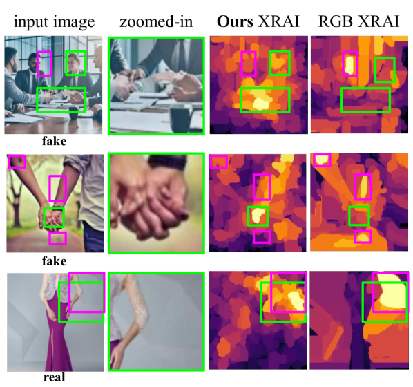
Figure 3: Saliency Analysis. Green boxes highlight the most salient regions according to our model and purple boxes for an equivalent RGB-only model. We use a post-hoc explainability technique, XRAI [29]. The regions of anatomical inconsistencies in fakes are most salient in our model.

Robustness and Interpretability. Table 5 shows that our method is sufficiently robust to in-the-wild transformations [20] such as JPEG re-compression and blur. Figure 3 shows that a model that uses inversion maps not only generalizes better but also focuses more on features that humans recognize as GenAI artifacts (e.g. malformed hands).

Discussion. Our results suggest that, while both our method and recent methods (UFD [37], DMDet [17]) consistently outperform older prior methods (CNNDet [54]) on prior academic benchmarks, recent methods struggle to maintain the same level of exceptional performance when evaluated against our new RIS-based evaluation benchmark, even when retrained on better data. Our method and some of the older baselines, on the other hand, perform well on both. We attribute this discrepancy to the drastic shift between real and fake images used in prior evaluation – suggesting that some of the recent methods were in part overfitting to the distributions of styles and content of natural images, which appears to be less of an issue for our method.

6 Conclusion

In this paper, we introduce FakeInversion: a GenAI detection method that uses text-conditioned inversion maps extracted from a pre-trained Stable Diffusion to achieve a new state-of-the-art at detecting images generated via unseen text-to-image diffusion models. We also propose SynRIS: a new challenging evaluation protocol that uses reverse image search to ensure that the evaluation is not biased towards any styles and themes. We show that the new protocol is also more reliable at evaluating detectors on images generated using proprietary models trained on unknown data. While FakeInversion improves upon the state-of-the-art on this challenging benchmark, there clearly remains much work to be done; the detection performance on the new evaluation benchmark is far from saturated. We invite future researchers to use these new datasets to explore, build, and deploy better GenAI detectors at scale, with confidence that their solutions will not favor any content and style.

Supplementary – Table of Contents

In this supplementary material, we provide following additional details regarding the proposed model and data:

• In Section A we describe how traing and eval data was obtained. Visualizations of real and fake image pairs for all evaluation datasets in the proposed SynRIS benchmark can be found in the end of the document in Fig. F.1-F.7.

• In Section B we provide a derivation of the relationship (8) from the main paper - connecting likelihood with inversion maps, DDIM discretization and reconstruction errors.

• In Section C we provide technical details of how our model was trained: architecture, inversion and captioning models we used.

• In Section D we provide extended evaluation results: Average Precision (AP) and overall accuracy for all evaluated methods, ROC, PR and DET curves, evaluation of robustness to prompt shift and fine-tuning, and the effect of text conditioning.

• In Section E we discuss how baselines were trained and issues we encountered when evaluating DIRE.

• In Section F, we include sample visualizations from the various datasets of our SynRIS benchmark.

Ethics and Limitations

The ultimate goal of this work is to prevent abuse and the spread of misinformation, an inherently ethical task. When generating our datasets, we sourced our prompts from an existing database. As such, some of the generated images may inadvertently contain inappropriate content. We explicitly address misalignment between fake and real images in our training and evaluation to ensure that the detector is not favouring any styles or themes to avoid marginalization of any groups.

While our method performs well at detecting images from existing diffusion models, this same performance may not transfer well to text-to-image models that do not make use of diffusion, such as text-to-image GANs (GigaGAN [28]) and transformers (Muse [15]). Training our model also requires significantly more compute than similar methods (CNNDetect [54], DMDetect [17]) since we must first pass all training images through our inversion pipeline.

Appendix A Data

In this section we discuss how training and evaluation datasets were generated. Our new training set along with all our RIS-based evaluation benchmark can be found at our project page: [will be released with camera ready].

A.1 Training Data

We train our method and other baselines on two different training sets: ProGAN + LSUN and DiffusionDB + LAION (DDB-L).

A.1.1 ProGAN+LSUN

Authors of CNNDetect [54] introduced this dataset along with their GAN detection method. This dataset consists of 360k real images from LSUN [59] and 360k fake images generated by ProGAN [30], each composed of 20 different classes. All real and fake images are 256x256 resolution.

A.1.2 Stable Diffusion+LAION

For this training set, we took random 300k fake images from DiffusionDB [56] and random 300k images from LAION [49] with predicted aesthetic scores of 6.25 or higher. Note that DiffusionDB consists of images from Stable Diffusion v1.

A.2 Evaluation Data - Fakes

This sections provides detail how each evaluation dataset’s fake images were obtained.

A.2.1 Imagen

We obtained Imagen images from authors of Imagen – they generated them using an internal closed API using the same prompt distribution that was used to train the Imagen model.

A.2.2 Midjourney

For our Midjourney images, we use this dataset on Hugging Face (link). These images were scraped from the Midjourney Discord server. This dataset includes a tag indicating whether or not the image was “upscaled” by the user. We choose images that had been upscaled since they are presumably of higher quality (since the user spent additional credits to upscale them).

A.2.3 DALL·E 3

For our DALL·E 3 images, we use this dataset on Hugging Face (link). These images were generated by users and shared on the LAION Discord server.

A.2.4 Kandinsky 2

For our Kandinsky 2 images, we use the Kandinsky 2.2 [51] model from Hugging Face (link), using the default parameters given in their usage example:

• prior_guidance_scale=1.0

• height=768

• width=768

• negative_prompt=‘‘low quality, bad quality’’

A.2.5 Kandinsky 3

For our Kandinsky 3 images, we use the Kandinsky 3 [10] model from Hugging Face (link), using the default parameters given in their usage example:

• num_inference_steps=50

A.2.6 PixArt-$\alpha$

For our PixArt-$\alpha$ [16] images, we use the 1024 resolution model from Hugging Face (link). All parameters are left as their defaults.

A.2.7 Playground 2.5

For our Playground 2.5 images, we use the Playground 2.5 [31] model from Hugging Face (link), using the default parameters given in their usage example:

• num_inference_steps

• guidance_scale=3

A.2.8 SDXL Direct Preference Optimization

For our SDXL-DPO images, we use the SDXL-DPO [53] model from Hugging Face (link), with the default parameters given in their usage example:

• guidance_scale=5

A.2.9 Stable Diffusion XL

For our SDXL images, we use the Stable Diffusion XL [41] model from Hugging Face (link), using both the base and refiner models with the default parameters given in their usage example:

• num_inference_steps=40

• denoising_end=0.8

• denoising_start=0.8

A.2.10 Segmind Mixture of Experts

For our Seg-MoE images, we use the SegMoE-4x2-v0 [58] model from Hugging Face (link), with the default parameters given in their usage example:

• negative_prompt=‘‘nsfw, bad quality, worse quality’’

• height=1024

• width=1024

• num_inference_steps=25

• guidance_scale=7.5

A.2.11 Segmind Stable Diffusion 1B

For our SSD-1B [21] images, we use the SSD-1B model from Hugging Face (link), using the default parameters given in their usage example:

• negative_prompt="ugly, blurry, poor quality"

A.2.12 Stable Cascade

For our Stable Cascade [39] images, we use the Stable Cascade model from Hugging Face (link), using the default parameters given in their usage example for the prior model:

• height=1024

• width=1024

• guidance_scale=4.0

• num_inference_steps=20

and decoder model:

• guidance_scale=0.0

• num_inference_steps=10

A.2.13 Segmind Vega

For our Segmind Vega [21] images, we use the Segmind Vega model from Hugging Face (link), using the default parameters given in their usage example:

• negative_prompt="(worst quality, low quality, illustration, 3d, 2d, painting, cartoons, sketch)"

A.2.14 Würstchen 2

For our Wüerstchen [39] images, we use the Wüerstchen v2 model from Hugging Face (link), using the default parameters given in their usage example:

• height=1024

• width=1024

• prior_guidance_scale=4.0

• decoder_guidance_scale=0.0

We will also include images and results from Wüerstchen v3, which is currently in beta development.

A.3 Evaluation Data - Reals

The corresponding real images for all of our evaluation sets were found via a reverse image search API provided by one of the major image search engines.

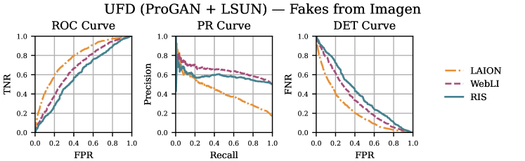
Figure A.1: Receiver Operating Characteristic (left) Precision-Recall (middle) and Detection Error Tradeoff (right) curves for detecting Imagen versus real images from its training set WebLI [60] (red), Reverse Image Search (green) and LAION (orange). These curves show that Imagen versus RIS is indeed a significantly harder task than Imagen versus LAION [49] and matches Imagen versus WebLI.

Appendix B Derivations

In this section we show the relationship between likelihood, DDIM inversion and DDIM reconstruction error. Notably, in the first approximation, it can be expressed using these terms without explicit dependency on model parameters $\theta$.

B.1 Derivation of Eq. 8

Given an appropriate change of variable $\bf{f}$ we know:

$$\log p(\bf{x})=\log p_{z}(\bf{f}^{-1}(x))+\log\det\operatorname{\bf J}[\bf f^{-1}](x)$$

Rewriting the negative log Jacobain determinant as:

$$-\log\det\operatorname{\bf J}[\bf f^{-1}](x)$$

$$= \log\det\operatorname{\bf J}[\bf f](f^{-1}(x))$$

$$= \operatorname{\bf Tr}\left(\log\operatorname{\bf J}[\bf f](f^{-1}(x))\right)$$

$$= \operatorname{\bf Tr}\left(\sum_{k=1}^{\infty}(-1)^{k+1}\frac{\left(\operatorname{\bf J}[\bf f](f^{-1}(x))-I)\right)^{k}}{k}\right)$$

(take the first term)

$$\approx \operatorname{\bf Tr}\left(\operatorname{\bf J}[\bf f](f^{-1}(x))-I\right)$$

$$\propto \operatorname{\bf Tr}\left(\operatorname{\bf J}[\bf f](f^{-1}(x))\right)$$

$$\text{(use Hutchinson estimator, assuming }\mu_{v}=0,\Sigma_{v}=I)$$

$$= \mathbb{E}_{\bf v}\langle{\bf v},\operatorname{\bf J}[\bf f](f^{-1}(x))\ \bf{v}\rangle$$

$$\text{(reparametrize with $\delta$ such that }\mu_{\delta}=0,\Sigma_{\delta}=\sigma_{\delta}I)$$

$$= \mathbb{E}_{\delta}\langle{\delta},\operatorname{\bf J}[\bf f](f^{-1}(x))\ \delta\rangle/\sigma_{\delta}^{2}$$

(take a single sample estimate)

$$\approx \langle{\delta},\operatorname{\bf J}[\bf f](f^{-1}(x))\ \delta\rangle/\|\delta\|^{2}$$

$$\text{(Taylor expansion of $\bf{f}$ around }\bf{f}^{-1}(x)\text{)}$$

$$\approx \langle\delta,\bf{f}(\bf{f}^{-1}(x)+\delta)-\bf{f}(\bf{f}^{-1}(x))\rangle/\|\delta\|^{2}$$

$$= \langle\delta,\bf{f}(\bf{f}^{-1}(x)+\delta)-x\rangle/\|\delta\|^{2}$$

and substituting

$$\bf{x}=x_{0}$$

$$\bf{f}^{-1}(x)=x_{T}$$

$$\bf{f}^{-1}(x)+\delta=\hat{x}_{T}$$

$$\bf{f}(\bf{f}^{-1}(x)+\delta)=\hat{x}_{0}$$

and assuming a small enough isotropic $\delta$, in the first approximation, we get:

$$\log p(\bf{x}_{0})\propto\log p_{z}(\bf{x}_{T})-\langle\delta,\hat{\bf{x}}_{0}-\bf{x}_{0}\rangle/\|\delta\|^{2}$$

Appendix C Training Details

In this section, we detail the various components of the pipeline used to train our detector.

C.1 Captioning

We use the BLIP-2, OPT-2.7b [32] model from Hugging Face (link) to caption our images before inversion and after and augmentations. Captioning is done after any augmentation since the augmentations could significantly change the caption (e.g., an RGB image converted to grayscale).

C.2 Inversion

We base our inversion process on Pix-to-Pix Zero [38], making use of the Hugging Face implementation (link) without the additional attention map guidance and other regularizers.

We first resize to 512$\times$512 and then invert all images (training and evaluation) using the same Stable Diffusion 1.5 [45] checkpoint from Hugging Face (link).

C.3 Training

The original images, inverted noise maps, and denoised reconstructions are then concatenated along the channel dimension and used as input to a ResNet-50 [22]. We train our detector for 25 Epochs, but most of the performance is gained in the first few. We otherwise use the same hyper-parameters as CNNDet [54].

Appendix D Extended Results

D.1 Extended metrics

In Table D.1 and Table D.2 we show AP and Acc@EER metrics for all experiments in addition to AUCROC. Figures Figures D.2, D.3, D.4, D.5, D.6 and D.7 show ROC, PR and DET curves for all compared classifiers.

Train Data	ProGAN + LSUN			Stable Diffusion + LAION
Eval Set   |   Model	CNNDet	UFD	Ours	CNNDet†	UFD†	Ours
DALL·E 2 [44]	0.499	0.694	0.867	0.653	0.750	0.751
DALL·E 3 [12]	0.473	0.384	0.625	0.703	0.474	0.756
Midjourney v5/6 [2]	0.498	0.419	0.736	0.602	0.555	0.643
Imagen [46]	0.474	0.582	0.759	0.705	0.553	0.791
Kandinsky 2 [51]	0.493	0.479	0.764	0.592	0.547	0.695
Kandinsky 3 [10]	0.491	0.470	0.860	0.654	0.605	0.755
PixArt-$\alpha$ [16]	0.490	0.502	0.871	0.623	0.625	0.744
Playground 2.5 [31]	0.510	0.462	0.778	0.556	0.571	0.617
SDXL-DPO [53]	0.495	0.475	0.849	0.829	0.683	0.874
SDXL [41]	0.506	0.470	0.777	0.799	0.651	0.792
Seg-MOE [58]	0.490	0.428	0.800	0.644	0.611	0.704
SSD-1B [21]	0.544	0.509	0.840	0.714	0.613	0.787
Stable-Cascade [39]	0.508	0.399	0.892	0.712	0.656	0.766
Segmind Vega [21]	0.524	0.475	0.834	0.723	0.612	0.796
Würstchen 2 [39]	0.508	0.592	0.803	0.600	0.670	0.712
DALL·E 2 [44] (A)	0.160	0.256	0.620	0.202	0.216	0.587
Craiyon [18] (A)	0.621	0.977	0.893	0.737	0.922	0.876
LDM [45] (A)	0.598	0.933	0.897	0.901	0.924	0.976
Average	0.493	0.528	0.804	0.664	0.624	0.757

Table D.1: Main Results – Detector Average Precision. In the main paper, we report the AUCROC metric when evaluating our classifiers. We report AP (Average Precision) here for completeness as well. We observe similar trends: our method performs best across nearly all datasets. ^∗Note: This DMDet classifier was trained with fakes from an LDM checkpoint rather than Stable Diffusion. ^†These models were re-trained by us.

Train Data	ProGAN + LSUN			Stable Diffusion + LAION
Eval Set   |   Model	CNNDet	UFD	Ours	CNNDet†	UFD†	Ours
DALL·E 2 [44]	0.470	0.674	0.773	0.624	0.700	0.678
DALL·E 3 [12]	0.435	0.371	0.592	0.659	0.473	0.698
Midjourney v5/6 [2]	0.490	0.413	0.661	0.595	0.558	0.606
Imagen [46]	0.470	0.580	0.706	0.674	0.538	0.720
Kandinsky 2 [51]	0.490	0.483	0.687	0.574	0.541	0.652
Kandinsky 3 [10]	0.481	0.478	0.766	0.609	0.600	0.684
PixArt-$\alpha$ [16]	0.485	0.504	0.769	0.591	0.606	0.669
Playground 2.5 [31]	0.508	0.477	0.707	0.553	0.562	0.591
SDXL-DPO [53]	0.486	0.473	0.764	0.761	0.647	0.801
SDXL [41]	0.497	0.473	0.688	0.735	0.620	0.737
Seg-MOE [58]	0.472	0.429	0.725	0.625	0.586	0.664
SSD-1B [21]	0.545	0.506	0.748	0.665	0.585	0.724
Stable-Cascade [39]	0.477	0.383	0.802	0.652	0.633	0.694
Segmind Vega [21]	0.522	0.476	0.741	0.676	0.587	0.733
Würstchen 2 [39]	0.504	0.580	0.715	0.580	0.640	0.658
DALL·E 2 [44] (A)	0.656	0.620	0.590	0.556	0.562	0.558
Craiyon [18] (A)	0.610	0.917	0.783	0.699	0.836	0.810
LDM [45] (A)	0.591	0.845	0.793	0.837	0.840	0.933
Average	0.510	0.538	0.723	0.648	0.617	0.700

Table D.2: Main Results – Acc @ Equal Error Rate. We further report Acc@EER here as an additional metric. We observe similar trends: our method performs best across nearly all datasets. ^∗Note: This DMDet classifier was trained with fakes from an LDM checkpoint rather than Stable Diffusion. ^†These models were re-trained by us.

D.2 Very Out-of-Distribution Data

The generators analyzed thus far are trained to be general aesthetic text-to-image models.

Here, we evaluate our model on models that have been fine-tuned generate images from very specific domains: Anime and Pokémon. Table D.3 shows that even when using low-quality training data (ProGAN), our model still generalizes to these very out-of-distribution domains while existing methods (UFD [37], CNNDet [54]) completely fail, even performing worse than random guessing.

	Detection Method
Eval Set	Ours	UFD	CNNDet
Anime	0.67	0.13	0.34
Pokémon	0.83	0.32	0.48

Table D.3: AUCROC. When trained on lower-quality data (ProGAN), existing methods (UFD [37], CNNDet [54]) completely fail to generalize to our extremely out-of-distribution datasets, even doing worse than randomly guessing. On the other hand, our method continues to generalize well.

D.3 Text-Conditioning

In Figure D.1, we show the effect of text-conditioning on the inversion-reconstruction process. By using text-conditioning, we recover a more faithful reconstruction of the input image, providing better signal for our model.

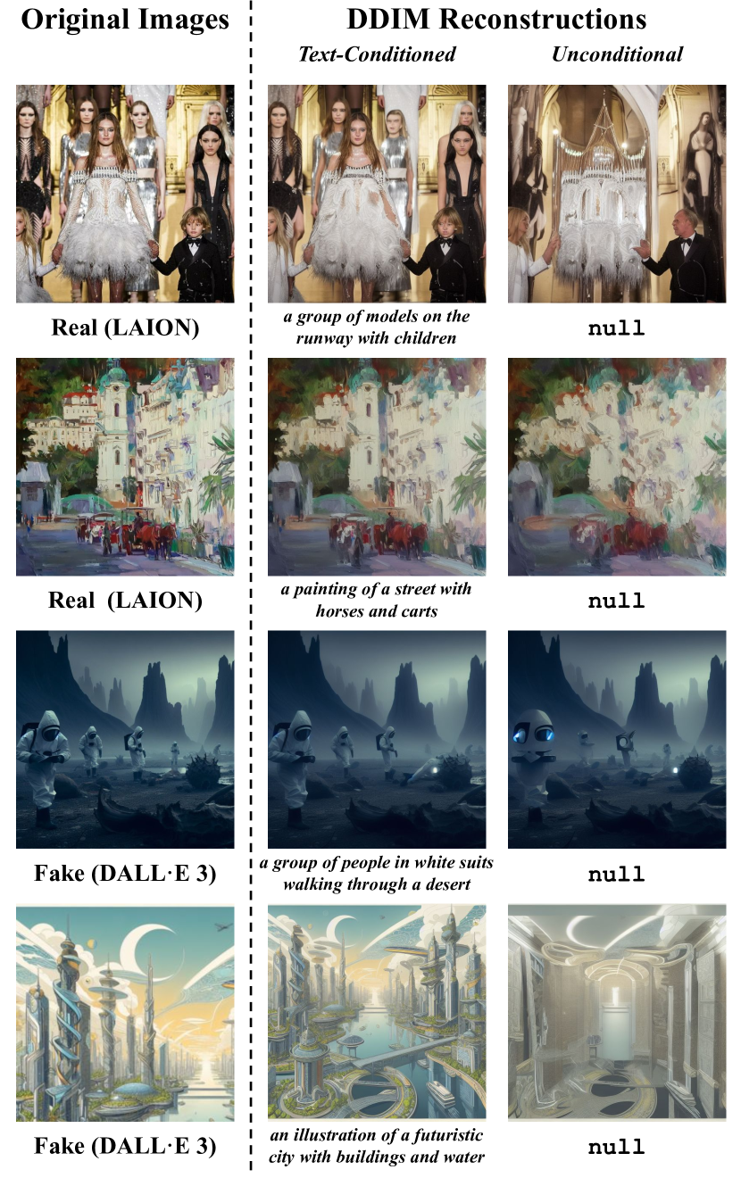
Figure D.1: Unconditional DDIM inversion and reconstruction catastrophically fails to reconstruct the original image. To remedy this, we predict a caption using BLIP 2 [32] and use this for text conditioning.

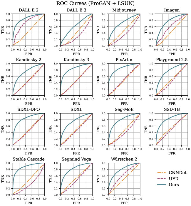
Figure D.2: ROC curves for all 15 of our SynRIS evaluation datasets. Models trained on ProGAN+LSUN.

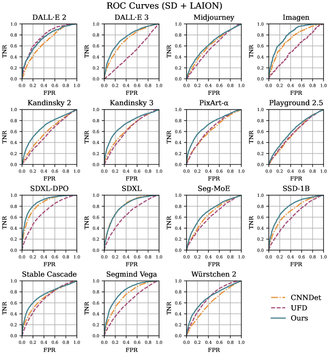
Figure D.3: ROC curves for all 15 of our SynRIS evaluation datasets. Models trained on SD+LAION.

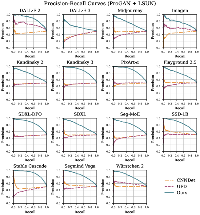
Figure D.4: Precision-Recall curves for all 15 of our SynRIS evaluation datasets. Models trained on ProGAN+LSUN.

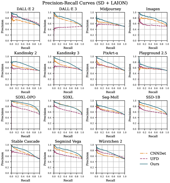
Figure D.5: Precision-Recall curves for all 15 of our SynRIS evaluation datasets. Models trained on SD+LAION.

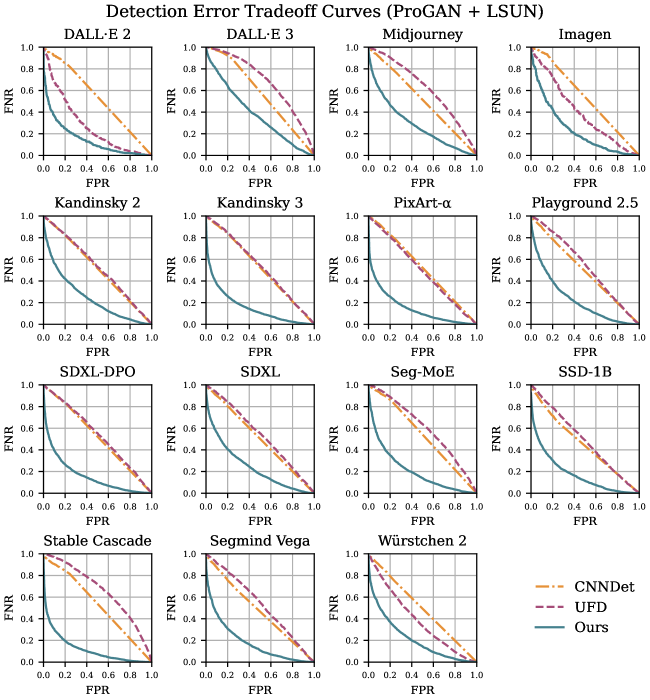
Figure D.6: Detection Error Tradeoff curves for all 15 of our SynRIS evaluation datasets. Models trained on ProGAN+LSUN.

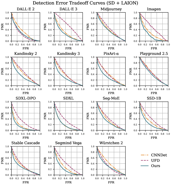
Figure D.7: Detection Error Tradeoff curves for all 15 of our SynRIS evaluation datasets. Models trained on SD+LAION.

Appendix E Baselines

E.1 DIRE [55]

The DIRE [55] paper reports almost perfect detection performance on all unseen test sets. However, after their code was released, several researchers noticed a fundamental issue with the training and evaluation setup present in their released code and checkpoints (link) causing the in-the-wild performance to drop to near-random levels. More specifically, all pre-processed images used for training are saved with the same extension as the source images. Since all input real images in the training set are saved as *.JPG files and all fake images are saved as *.PNG files, all real DIRE images used to train and evaluate the network were embedded with JPEG artifacts while the non of the fake images used for training and evaluation were. As such, the model seemingly learned to detect the presence of JPEG artifacts. This holds even for the robustness experiments since augmented real and fake images are also saved as JPG and PNG respectively. In all of our datasets, both real and fake images are saved as lossless *.PNG files, explaining DIRE’s poor performance on all our test sets. To honor the contribution of DIRE authors, we conducted an ablation that used the exact same absolute residuals signals as reported in DIRE paper. It is evident from our results that the inversion signals we propose in this paper perform much better then DIRE signals across all evaluation benchmarks.

E.2 CNNDet [54]

We trained using the original CNNDet training code (link) using following default parameters.

• --name blur_jpg_prob=0.5

• --blur_prob=0.5

• --blur_sigma=0.0,0.3

• --jpeg_prob=0.5

• --jpeg_method=cv2,pil

• --jpeg_qual=30,100

All training and eval images are resized to 256$\times$256 and saved as .PNG files.

E.3 UFD [37]

We trained using the original UFD training code (link) using following default parameters.

• --name=clip_vitl14

• --wang2020_data_path=datasets

• --data_mode=wang2020

• --arch=CLIP:ViT-L/14

• --fix_backbone

All training and eval images are resized to 256$\times$256 and saved as .PNG files.

Appendix F SynRIS Visualization

Figures F.1, F.2, F.3 and F.4 contain samples from our evaluation sets using closed-source models. Figures F.5, F.6, F.7, F.8, F.9, F.10, F.11, F.12, F.13, F.14 and F.15 contain samples from our evaluation sets using open-source models. The corresponding images in each of these open-source model figures were generates using the same prompts. The top panel consists of fake images either found online or generated by us, and the bottom panel are the corresponding real images found via reverse image search.

Figures F.16 and F.17 contain samples from our Pokémon and Anime datasets respectively. The real images were taken from a source dataset [40, 6] and the attached captions were used to generate the fake images with SD Pokémon Diffusers [4] and Animagine [7].

Fake (Imagen [46])

Real (Reverse Image Search)

Figure F.1: Top: A sample of fake Imagen [46] images we generated for our dataset. Bot: Corresponding real images found via RIS.

Fake (Midjourney [2])

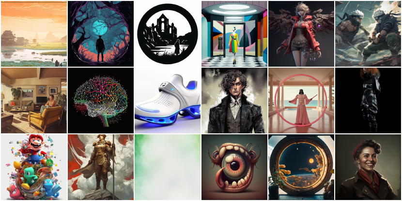
Real (Reverse Image Search)

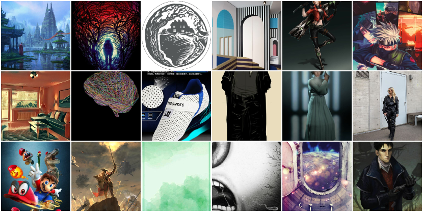
Figure F.2: Top: A sample of fake Midjourney [12] images taken from Hugging Face (link). Bot: Corresponding real images found via RIS.

Fake (DALL·E 2 [44])

Real (Reverse Image Search)

Figure F.3: Top: A sample of fake DALL·E 2 [44] images taken from the DMDetect [17] repo (link). Bot: Corresponding real images found via RIS.

Fake (DALL·E 3 [12])

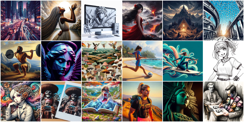
Real (Reverse Image Search)

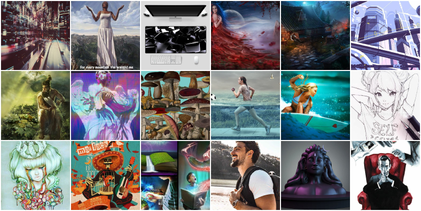
Figure F.4: Top: A sample of fake DALL·E 3 [12] images taken from Hugging Face (link). Bot: Corresponding real images found via RIS.

Fake (Kandinsky 2 [51])

Real (Reverse Image Search)

Figure F.5: Top: A sample of fake Kandinsky 2 [51] images we generated for our dataset. Bot: Corresponding real images found via RIS.

Fake (Kandinsky 3 [10])

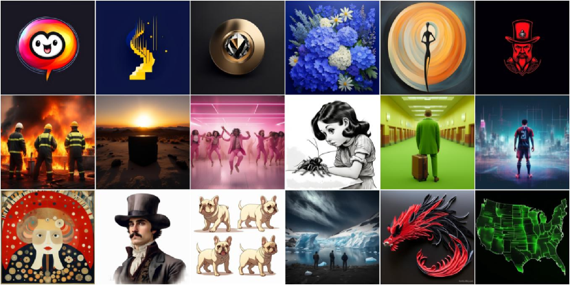
Real (Reverse Image Search)

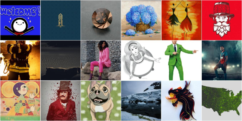
Figure F.6: Top: A sample of fake Kandinsky 3 [10] images we generated for our dataset. Bot: Corresponding real images found via RIS.

Fake (PixArt-$\alpha$ [16])

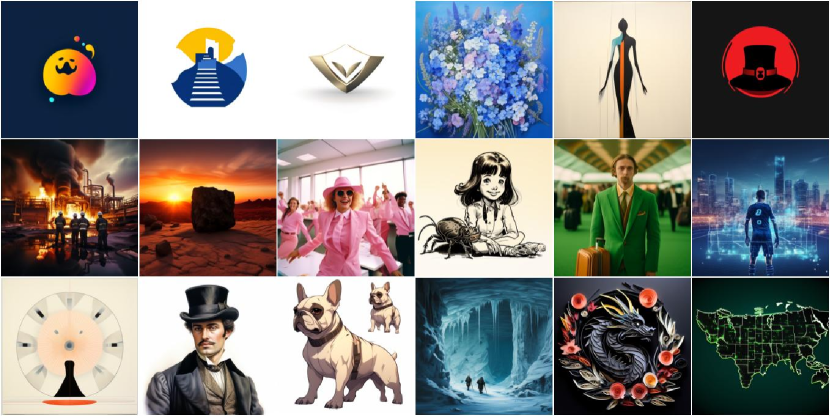
Real (Reverse Image Search)

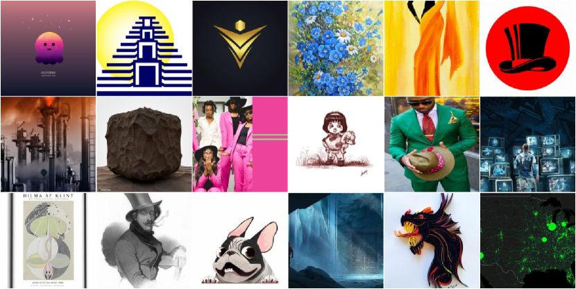
Figure F.7: Top: A sample of fake PixArt-$\alpha$ [16] images we generated for our dataset. Bot: Corresponding real images found via RIS.

Fake (Playground 2.5 [31])

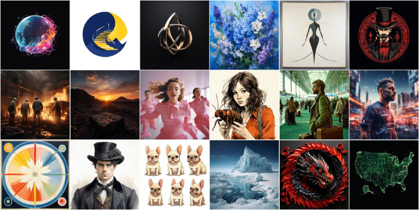
Real (Reverse Image Search)

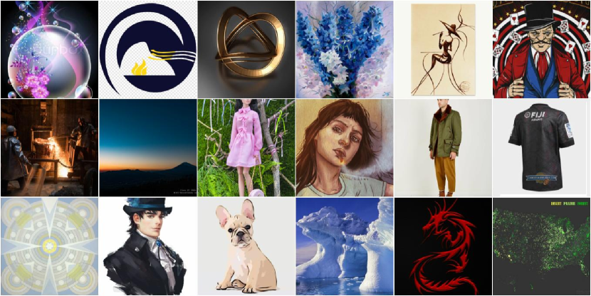
Figure F.8: Top: A sample of fake Playground [31] images we generated for our dataset. Bot: Corresponding real images found via RIS.

Fake (SDXL-DPO [53])

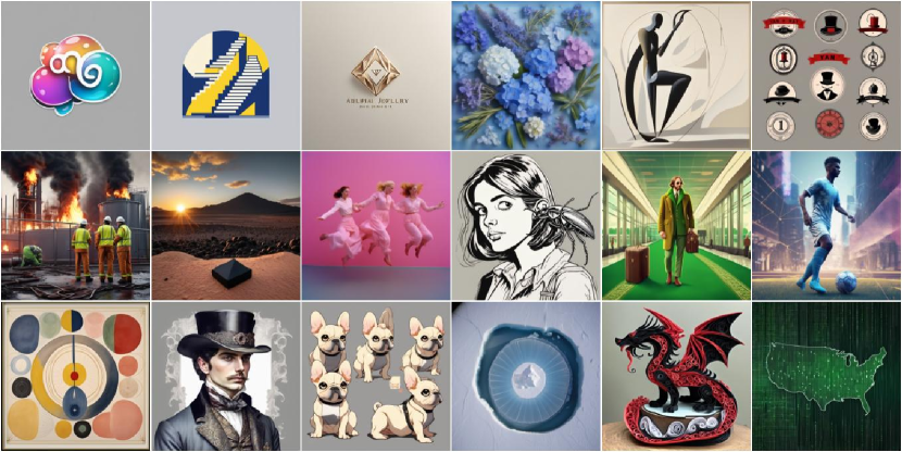
Real (Reverse Image Search)

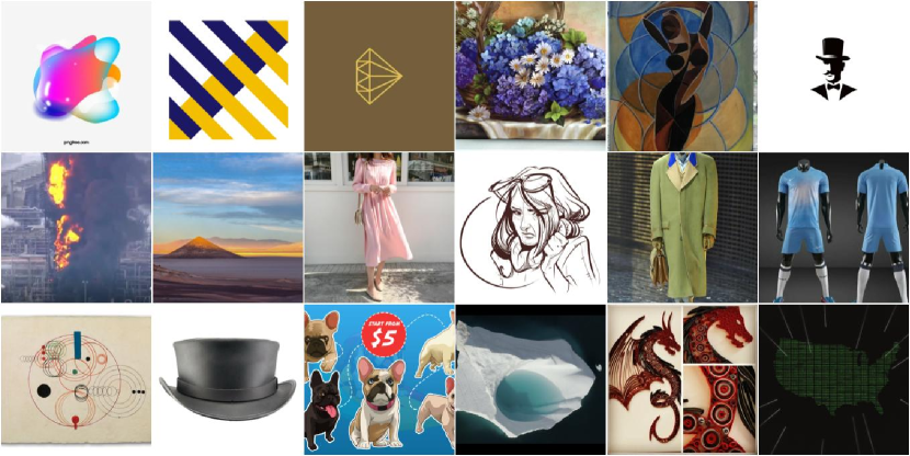
Figure F.9: Top: A sample of fake SDXL-DPO [53] images we generated for our dataset. Bot: Corresponding real images found via RIS.

Fake (SDXL [41])

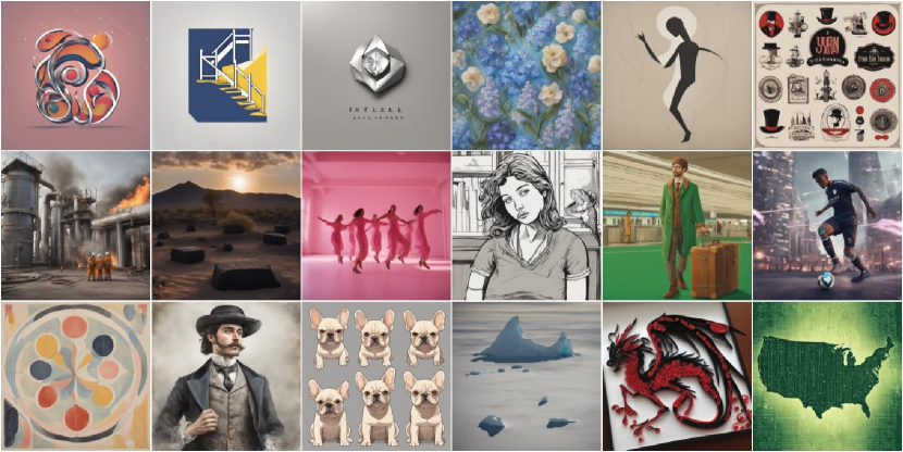
Real (Reverse Image Search)

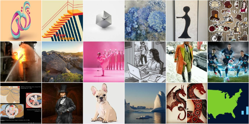
Figure F.10: Top: A sample of fake SDXL [41] images we generated for our dataset. Bot: Corresponding real images found via RIS.

Fake (Seg-MoE [58])

Real (Reverse Image Search)

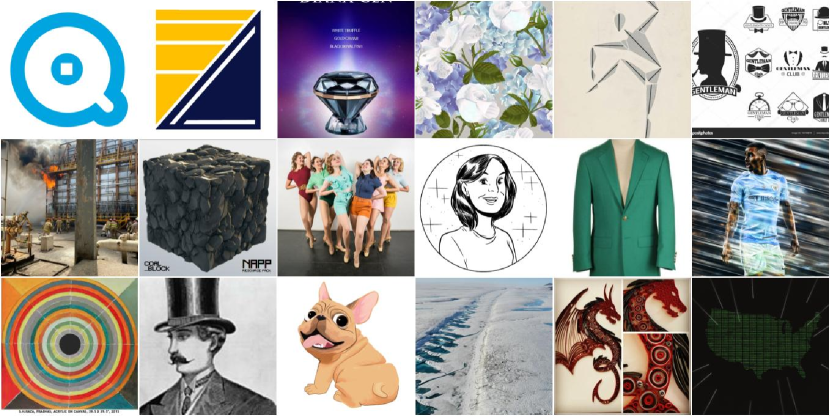
Figure F.11: Top: A sample of fake Seg-MoE [58] images we generated for our dataset. Bot: Corresponding real images found via RIS.

Fake (SSD-1B [21])

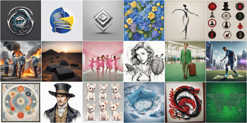
Real (Reverse Image Search)

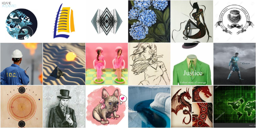
Figure F.12: Top: A sample of fake SSD-1B [21] images we generated for our dataset. Bot: Corresponding real images found via RIS.

Fake (Stable-Cascade [39])

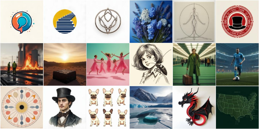
Real (Reverse Image Search)

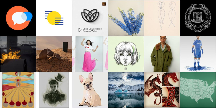
Figure F.13: Top: A sample of fake Stable-Cascade [39] images we generated for our dataset. Bot: Corresponding real images found via RIS.

Fake (Segmind Vega [21])

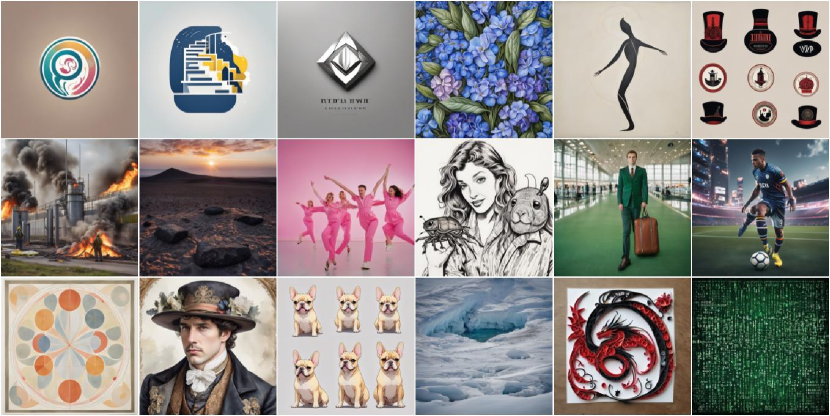
Real (Reverse Image Search)

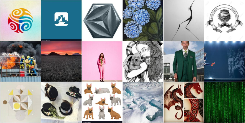
Figure F.14: Top: A sample of fake Segmind Vega [21] images we generated for our dataset. Bot: Corresponding real images found via RIS.

Fake (Würstchen 2 [39])

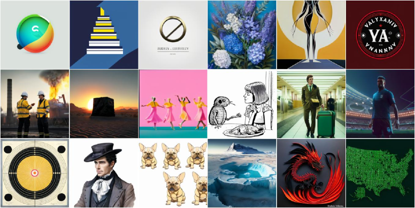
Real (Reverse Image Search)

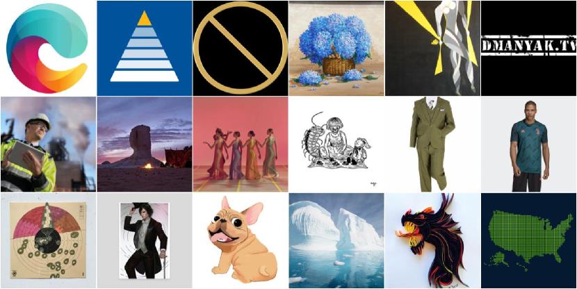
Figure F.15: Top: A sample of fake Würstchen 2 [39] images we generated for our dataset. Bot: Corresponding real images found via RIS.

Fake (SD Pokémon Diffusers [4])

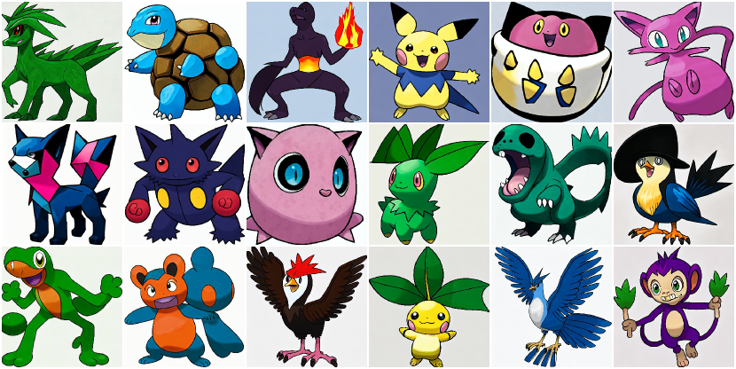
Real (Pokémon [5])

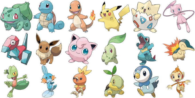
Figure F.16: Top: A sample of fake Pokémon images we generated for our dataset. Bot: Corresponding real images. The above fake images were generated using the BLIP [32] captions of these real images as prompts [40].

Fake (Animagine XL 2.0 [7])

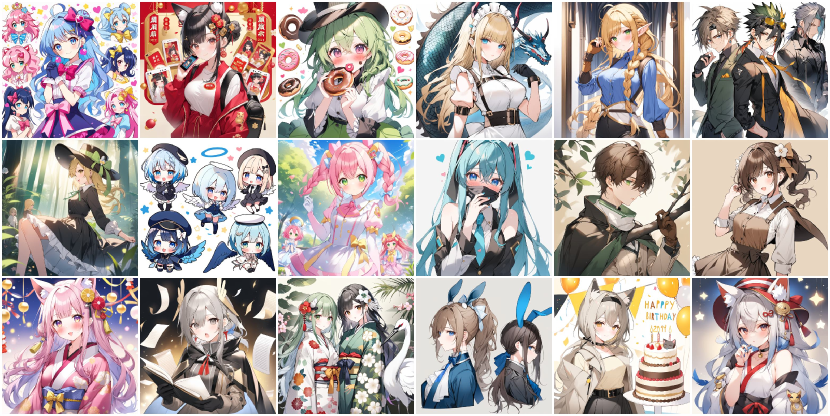
Real (Danbooru [6])

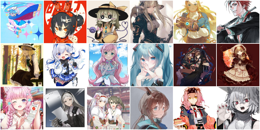
Figure F.17: Top: A sample of fake Anime images we generated for our dataset. Bot: Corresponding real images from the (SFW) Danbooru 2022 dataset [6]. The above fake images were generated using the Danbooru tags of these real images as prompts.

References

- [1] Deepfakes could supercharge health care’s misinformation problem. https://www.axios.com/2023/11/14/ai-deepfake-health-misinformation-fake-pictures-videos.
- [2] Midjourney. https://www.midjourney.com/.
- [3] An a.i.-generated picture won an art prize. artists aren’t happy. https://www.nytimes.com/2022/09/02/technology/ai-artificial-intelligence-artists.html.
- [4] Sd pokémon diffusers. https://huggingface.co/lambdalabs/sd-pokemon-diffusers.
- [5] Pokémon. pokemon.com.
- dan [2022] Danbooru 2022 dataset. https://huggingface.co/datasets/animelover/danbooru2022, 2022.
- ani [2023] Animagine XL 2.0. https://huggingface.co/Linaqruf/animagine-xl-2.0, 2023.
- dal [2023] laion/dalle-3-dataset · datasets at hugging face, 2023.
- wan [2023] wanng/midjourney-v5-202304-clean · datasets at hugging face, 2023.
- Arkhipkin et al. [2023] Vladimir Arkhipkin, Andrei Filatov, Viacheslav Vasilev, Anastasia Maltseva, Said Azizov, Igor Pavlov, Julia Agafonova, Andrey Kuznetsov, and Denis Dimitrov. Kandinsky 3.0 technical report, 2023.
- Bau et al. [2019] David Bau, Jun-Yan Zhu, Jonas Wulff, William Peebles, Hendrik Strobelt, Bolei Zhou, and Antonio Torralba. Seeing what a gan cannot generate. In ICCV, 2019.
- [12] James Betker, Gabriel Goh, Li Jing, Tim Brooks, Jianfeng Wang, Linjie Li, Long Ouyang, Juntang Zhuang, Joyce Lee, Yufei Guo, Wesam Manassra, Prafulla Dhariwal, Casey Chu, and Yunxin Jiao. Improving image generation with better captions. https://cdn.openai.com/papers/dall-e-3.pdf.
- Bińkowski et al. [2018] Mikołaj Bińkowski, Danica J Sutherland, Michael Arbel, and Arthur Gretton. Demystifying mmd gans. arXiv preprint arXiv:1801.01401, 2018.
- Chai et al. [2020] Lucy Chai, David Bau, Ser-Nam Lim, and Phillip Isola. What makes fake images detectable? understanding properties that generalize. In ECCV, 2020.
- Chang et al. [2023] Huiwen Chang, Han Zhang, Jarred Barber, AJ Maschinot, Jose Lezama, Lu Jiang, Ming-Hsuan Yang, Kevin Murphy, William T Freeman, Michael Rubinstein, et al. Muse: Text-to-image generation via masked generative transformers. arXiv preprint arXiv:2301.00704, 2023.
- Chen et al. [2023] Junsong Chen, Jincheng Yu, Chongjian Ge, Lewei Yao, Enze Xie, Yue Wu, Zhongdao Wang, James Kwok, Ping Luo, Huchuan Lu, et al. Pixart-alpha: Fast training of diffusion transformer for photorealistic text-to-image synthesis. arXiv preprint arXiv:2310.00426, 2023.
- Corvi et al. [2023] Riccardo Corvi, Davide Cozzolino, Giada Zingarini, Giovanni Poggi, Koki Nagano, and Luisa Verdoliva. On the detection of synthetic images generated by diffusion models. In ICASSP, 2023.
- Dayma et al. [2021] Boris Dayma, Suraj Patil, Pedro Cuenca, Khalid Saifullah, Tanishq Abraham, Phúc Lê Khac, Luke Melas, and Ritobrata Ghosh. Dall-e mini, 2021.
- Epstein et al. [2023] David C. Epstein, Ishan Jain, Oliver Wang, and Richard Zhang. Online detection of ai-generated images. In ICCV Workshop, 2023.
- Frank et al. [2020] Joel Frank, Thorsten Eisenhofer, Lea Schönherr, Asja Fischer, Dorothea Kolossa, and Thorsten Holz. Leveraging frequency analysis for deep fake image recognition. In ICML, 2020.
- Gupta et al. [2024] Yatharth Gupta, Vishnu V. Jaddipal, Harish Prabhala, Sayak Paul, and Patrick Von Platen. Progressive knowledge distillation of stable diffusion xl using layer level loss, 2024.
- He et al. [2016] Kaiming He, Xiangyu Zhang, Shaoqing Ren, and Jian Sun. Deep residual learning for image recognition. In Proceedings of the IEEE conference on computer vision and pattern recognition, pages 770–778, 2016.
- Heusel et al. [2017] Martin Heusel, Hubert Ramsauer, Thomas Unterthiner, Bernhard Nessler, and Sepp Hochreiter. Gans trained by a two time-scale update rule converge to a local nash equilibrium. NeurIPS, 2017.
- Ho and Salimans [2022] Jonathan Ho and Tim Salimans. Classifier-free diffusion guidance. arXiv preprint arXiv:2207.12598, 2022.
- Ho et al. [2020] Jonathan Ho, Ajay Jain, and Pieter Abbeel. Denoising diffusion probabilistic models. NeurIPS, 2020.
- Huszár [2015] Ferenc Huszár. How (not) to train your generative model: Scheduled sampling, likelihood, adversary? arXiv preprint arXiv:1511.05101, 2015.
- Ju et al. [2022] Yan Ju, Shan Jia, Lipeng Ke, Hongfei Xue, Koki Nagano, and Siwei Lyu. Fusing global and local features for generalized ai-synthesized image detection. In ICIP, 2022.
- Kang et al. [2023] Minguk Kang, Jun-Yan Zhu, Richard Zhang, Jaesik Park, Eli Shechtman, Sylvain Paris, and Taesung Park. Scaling up gans for text-to-image synthesis. In CVPR, 2023.
- Kapishnikov et al. [2019] Andrei Kapishnikov, Tolga Bolukbasi, Fernanda Viégas, and Michael Terry. Xrai: Better attributions through regions. In ICCV, 2019.
- Karras et al. [2017] Tero Karras, Timo Aila, Samuli Laine, and Jaakko Lehtinen. Progressive growing of gans for improved quality, stability, and variation. ICML, abs/1710.10196, 2017.
- Li et al. [2024] Daiqing Li, Aleks Kamko, Ehsan Akhgari, Ali Sabet, Linmiao Xu, and Suhail Doshi. Playground v2.5: Three insights towards enhancing aesthetic quality in text-to-image generation, 2024.
- Li et al. [2023] Junnan Li, Dongxu Li, Silvio Savarese, and Steven Hoi. Blip-2: Bootstrapping language-image pre-training with frozen image encoders and large language models. arXiv preprint arXiv:2301.12597, 2023.
- Lin et al. [2014] Tsung-Yi Lin, Michael Maire, Serge Belongie, James Hays, Pietro Perona, Deva Ramanan, Piotr Dollár, and C Lawrence Zitnick. Microsoft coco: Common objects in context. In ECCV, 2014.
- Lu et al. [2022] Cheng Lu, Yuhao Zhou, Fan Bao, Jianfei Chen, Chongxuan Li, and Jun Zhu. Dpm-solver: A fast ode solver for diffusion probabilistic model sampling in around 10 steps. NeurIPS, 2022.
- Marra et al. [2019] Francesco Marra, Diego Gragnaniello, Luisa Verdoliva, and Giovanni Poggi. Do gans leave artificial fingerprints? In IEEE conference on multimedia information processing and retrieval (MIPR), 2019.
- Mokady et al. [2023] Ron Mokady, Amir Hertz, Kfir Aberman, Yael Pritch, and Daniel Cohen-Or. Null-text inversion for editing real images using guided diffusion models. In CVPR, 2023.
- Ojha et al. [2023] Utkarsh Ojha, Yuheng Li, and Yong Jae Lee. Towards universal fake image detectors that generalize across generative models. In CVPR, 2023.
- Parmar et al. [2023] Gaurav Parmar, Krishna Kumar Singh, Richard Zhang, Yijun Li, Jingwan Lu, and Jun-Yan Zhu. Zero-shot image-to-image translation. In ACM TOG, 2023.
- Pernias et al. [2023] Pablo Pernias, Dominic Rampas, Mats L. Richter, Christopher Pal, and Marc Aubreville. Wuerstchen: Efficient pretraining of text-to-image models, 2023.
- Pinkney [2022] Justin N. M. Pinkney. Pokemon blip captions. https://huggingface.co/datasets/lambdalabs/pokemon-blip-captions/, 2022.
- Podell et al. [2023] Dustin Podell, Zion English, Kyle Lacey, Andreas Blattmann, Tim Dockhorn, Jonas Müller, Joe Penna, and Robin Rombach. Sdxl: Improving latent diffusion models for high-resolution image synthesis. arXiv preprint arXiv:2307.01952, 2023.
- Radford et al. [2021] Alec Radford, Jong Wook Kim, Chris Hallacy, Aditya Ramesh, Gabriel Goh, Sandhini Agarwal, Girish Sastry, Amanda Askell, Pamela Mishkin, Jack Clark, et al. Learning transferable visual models from natural language supervision. In ICML, 2021.
- Ramesh et al. [2021] Aditya Ramesh, Mikhail Pavlov, Gabriel Goh, Scott Gray, Chelsea Voss, Alec Radford, Mark Chen, and Ilya Sutskever. Zero-shot text-to-image generation. In ICML, 2021.
- Ramesh et al. [2022] Aditya Ramesh, Prafulla Dhariwal, Alex Nichol, Casey Chu, and Mark Chen. Hierarchical text-conditional image generation with clip latents. arXiv preprint arXiv:2204.06125, 2022.
- Rombach et al. [2022] Robin Rombach, Andreas Blattmann, Dominik Lorenz, Patrick Esser, and Björn Ommer. High-resolution image synthesis with latent diffusion models. In CVPR, 2022.
- Saharia et al. [2022] Chitwan Saharia, William Chan, Saurabh Saxena, Lala Li, Jay Whang, Emily L Denton, Kamyar Ghasemipour, Raphael Gontijo Lopes, Burcu Karagol Ayan, Tim Salimans, et al. Photorealistic text-to-image diffusion models with deep language understanding. NeurIPS, 2022.
- Salimans and Ho [2022] Tim Salimans and Jonathan Ho. Progressive distillation for fast sampling of diffusion models. In ICLR, 2022.
- Schaefer and Stich [2003] Gerald Schaefer and Michal Stich. Ucid: An uncompressed color image database. In Storage and retrieval methods and applications for multimedia 2004. SPIE, 2003.
- Schuhmann et al. [2022] Christoph Schuhmann, Romain Beaumont, Richard Vencu, Cade Gordon, Ross Wightman, Mehdi Cherti, Theo Coombes, Aarush Katta, Clayton Mullis, Mitchell Wortsman, et al. Laion-5b: An open large-scale dataset for training next generation image-text models. NeurIPS, 2022.
- Sha et al. [2023] Zeyang Sha, Zheng Li, Ning Yu, and Yang Zhang. De-fake: Detection and attribution of fake images generated by text-to-image generation models, 2023.
- Shakhmatov et al. [2023] Arseniy Shakhmatov, Anton Razzhigaev, Aleksandr Nikolich, Vladimir Arkhipkin, Igor Pavlov, Andrey Kuznetsov, and Denis Dimitrov. kandinsky 2.2, 2023.
- Song et al. [2020] Jiaming Song, Chenlin Meng, and Stefano Ermon. Denoising diffusion implicit models. In ICLR, 2020.
- Wallace et al. [2023] Bram Wallace, Meihua Dang, Rafael Rafailov, Linqi Zhou, Aaron Lou, Senthil Purushwalkam, Stefano Ermon, Caiming Xiong, Shafiq Joty, and Nikhil Naik. Diffusion model alignment using direct preference optimization. arXiv preprint arXiv:2311.12908, 2023.
- Wang et al. [2020] Sheng-Yu Wang, Oliver Wang, Richard Zhang, Andrew Owens, and Alexei A Efros. Cnn-generated images are surprisingly easy to spot…for now. In CVPR, 2020.
- Wang et al. [2023] Zhendong Wang, Jianmin Bao, Wengang Zhou, Weilun Wang, Hezhen Hu, Hong Chen, and Houqiang Li. Dire for diffusion-generated image detection. ICCV, 2023.
- Wang et al. [2022] Zijie J Wang, Evan Montoya, David Munechika, Haoyang Yang, Benjamin Hoover, and Duen Horng Chau. Diffusiondb: A large-scale prompt gallery dataset for text-to-image generative models. arXiv preprint arXiv:2210.14896, 2022.
- wangjunjie [2023] wangjunjie. midjourney-v5-202304-clean. https://huggingface.co/datasets/wanng/midjourney-v5-202304-clean, 2023.
- Yatharth Gupta [2024] Harish Prabhala Yatharth Gupta, Vishnu V Jaddipal. Segmoe: Segmind mixture of diffusion experts. https://github.com/segmind/segmoe, 2024.
- Yu et al. [2015] Fisher Yu, Ari Seff, Yinda Zhang, Shuran Song, Thomas Funkhouser, and Jianxiong Xiao. Lsun: Construction of a large-scale image dataset using deep learning with humans in the loop. arXiv preprint arXiv:1506.03365, 2015.
- Yu et al. [2022] Jiahui Yu, Yuanzhong Xu, Jing Yu Koh, Thang Luong, Gunjan Baid, Zirui Wang, Vijay Vasudevan, Alexander Ku, Yinfei Yang, Burcu Karagol Ayan, Ben Hutchinson, Wei Han, Zarana Parekh, Xin Li, Han Zhang, Jason Baldridge, and Yonghui Wu. Scaling autoregressive models for content-rich text-to-image generation. TMLR, 2022.
- Zhang et al. [2019] Xu Zhang, Svebor Karaman, and Shih-Fu Chang. Detecting and simulating artifacts in gan fake images. In IEEE international workshop on information forensics and security (WIFS), 2019.