Optimizing the auxetic behavior of anisotropic laminates

Abstract

Anisotropic laminates with a negative Poisson’s ratio for at least some directions are called auxetic. In this paper, we consider the conditions for optimizing the auxeticity of an orthotropic laminate, namely: for a laminate composed by a given material, (i) how to obtain the lowest, i.e. the highest negative, Poisson’s ratio and (ii) how to maximize the auxetic zone, i.e. the set of directions where the Poisson’s ratio is negative. It is shown that in both the cases the optimal solution is found on the boundary of the feasible domain and in particular that it can be obtained using angle-ply sequences of identical layers. The polar method with dimensionless moduli is employed for representing the anisotropic behavior of the laminate, which allows, on the one hand, to reduce the dimensionality of the problem and, on the other hand, to have an effective mathematical representation of anisotropy by dimensionless invariants.

Key words: Poisson’s ratio, auxeticity, anisotropy, composite laminates, polar formalism, angle-ply laminates, optimization

1 Introduction

Auxeticity is the property of having a negative Poisson’s ratio, [1]. It is well known that an auxetic behavior is theoretically possible for isotropic materials, see e.g. [2, 3, 4], and that it can be obtained using materials having some special kind of microstructure (literature is very wide on this topic, some rather complete reviews on the matter can be found in [5] or [6]). In the case of anisotropic materials, the Poisson’s coefficients are anisotropic properties too and by consequence it is physically possible that they take negative values at some directions. In other words, auxeticity of anisotropic materials is an anisotropic property. When anisotropic layers are used in the fabrication of laminates, the mechanical properties of theses ones can be tailored by an appropriate choice of the orientation angles of the plies, see e.g. [7, 8, 9]. Hence, also auxeticity can be tailored, at least for some constituent materials. The possibility of obtaining auxetic orthotropic laminates has been treated in [10], where it has been shown which are the conditions on the mechanical properties of the constituent layer that are needed to fabricate, by an appropriate tailoring of the orientations, a laminate that has, for its in-plane behavior, a negative Poisson’s ratio at some directions.

In this paper, we complete the study considering two optimization problems concerning auxetic orthotropic laminates: for a given constituent layer, what are the conditions to obtain (i) the lowest, negative, in-plane Poisson’s ratio $\nu_{12}$ or (ii) the largest auxetic zone, i.e. the set of directions where $\nu_{12}<0$? The first problem has already been considered by Miki and Murotsu, in a seminal paper on auxetic laminates, [11], and later on by Zhang et al., [12]. Miki and Murotsu used a numerical optimization technique and argued that the maximization of $\nu_{12}$, that in their paper is indicated by $\nu_{21}$, can be obtained using angle-ply laminates, while the minimum is obtained still using two different orientations, but with unbalanced laminates, that hence are not orthotropic. Zhang et al. considered exclusively in-plane orthotropic laminates, assumed, without proving, that in this case the minimum of $\nu_{12}$ can be attained using angle-ply laminates and gave an approximated analytical expression for the gap angle between the two sets of layers for a minimization problem not clearly defined. The second problem is apparently still untreated in the literature.

In this paper we use the polar formalism, introduced in 1979 by G. Verchery, [13], particularly interesting as it makes use of invariants and of angles to represent the elastic properties. This method is very effective also in exploring unconventional mechanical situations, like the case of auxetic materials or also other more strange situations, see e.g. [14]. In particular, like in [10], we introduce dimensionless polar parameters, which allows to reduce the mathematical dimensionality of the problem. We show that the minimum $\nu_{12}$ and the widest angular range where $\nu_{12}<0$ can be obtained using angle-ply laminates and we give also an analytical expression for the optimal solution of the second problem.

2 Basic relations

2.1 Polar expression of the Poisson’s ratio

We consider an anisotropic ply in a plane-stress state, we fix a frame $\{x_{1},x_{2}\}$ and denote by $\mathbb{S}$ and $\mathbb{Q}=\mathbb{S}^{-1}$ respectively the compliance and the reduced stiffness tensors. Then, [15, 16, 7, 17],

$$\nu_{12}(\theta):=-\frac{\mathbb{S}_{12}(\theta)}{\mathbb{S}_{11}(\theta)}$$ (1)

is the in-plane Poisson’s ratio for the direction inclined of $\theta$ on the $x_{1}-$axis. Because $\mathbb{S}_{11}(\theta)>0\ \forall\theta$,

$$\nu_{12}(\theta)<0\iff\mathbb{S}_{12}(\theta)>0.$$ (2)

In the polar formalism, [18, 19]

$$\nu_{12}(\theta)=\frac{t_{0}-2t_{1}+r_{0}\cos 4(\varphi_{0}-\theta)}{t_{0}+2t_{1}+r_{0}\cos 4(\varphi_{0}-\theta)+4r_{1}\cos 2(\varphi_{1}-\theta)},$$ (3)

with $t_{0},t_{1},r_{0},r_{1}$ non-negative tensor invariants of $\mathbb{S}$ while $\varphi_{0},\varphi_{1}$ are polar angles whose difference is the fifth invariant of $\mathbb{S}$. Because we investigate the auxeticity of a laminate, whose elastic behavior is obtained homogenizing the reduced stiffnesses of the layers, it is worth to express $\nu_{12}(\theta)$ as function of the polar invariants of $\mathbb{Q}$. To this end, we express the polar parameters of $\mathbb{S}$ by those of $\mathbb{Q}$, [19]:

$$\begin{array}[]{l}t_{0}=2\dfrac{T_{0}T_{1}-R_{1}^{2}}{\varDelta},\vskip 6.0pt plus 2.0pt minus 2.0pt\\ t_{1}=\dfrac{T_{0}^{2}-R_{0}^{2}}{2\varDelta},\vskip 6.0pt plus 2.0pt minus 2.0pt\\ r_{0}\mathrm{e}^{4\mathrm{i}\varphi_{0}}=\dfrac{2}{\varDelta}(R_{1}^{2}\mathrm{e}^{4\mathrm{i}\varPhi_{1}}-T_{1}R_{0}\mathrm{e}^{4\mathrm{i}\varPhi_{0}}),\vskip 6.0pt plus 2.0pt minus 2.0pt\\ r_{1}\mathrm{e}^{2\mathrm{i}\varphi_{1}}=\dfrac{R_{1}\mathrm{e}^{2\mathrm{i}\varPhi_{1}}}{\varDelta}\left[R_{0}\mathrm{e}^{4\mathrm{i}\varPhi}-T_{0}\right].\end{array}$$ (4)

Here, $T_{0},T_{1},R_{0},R_{1}$ are the (non-negative) polar invariant moduli of $\mathbb{Q}$ and $\varPhi_{0},\varPhi_{1}$ the two polar angles of $\mathbb{Q}$, whose difference is

$$\varPhi:=\varPhi_{0}-\varPhi_{1},$$ (5)

which is the fifth independent invariant of $\mathbb{Q}$. $\varDelta$ is the quantity

$$\varDelta=4T_{1}(T_{0}^{2}-R_{0}^{2})-8R_{1}^{2}[T_{0}-R_{0}\cos 4\varPhi],$$ (6)

which actually coincides with the determinant of $\mathbb{Q}$, and as such is itself a positive invariant. Some simple passages give

$$\nu_{12}(\theta)=\frac{2(T_{0}T_{1}{-}R_{1}^{2}){-}T_{0}^{2}{+}R_{0}^{2}{+}2[R_{1}^{2}\cos 4(\varPhi_{1}{-}\theta){-}T_{1}R_{0}\cos 4(\varPhi_{0}{-}\theta)]}{2(T_{0}T_{1}{-}R_{1}^{2}){+}T_{0}^{2}{-}R_{0}^{2}{+}2[R_{1}^{2}\cos 4(\varPhi_{1}{-}\theta){-}T_{1}R_{0}\cos 4(\varPhi_{0}{-}\theta)]{+}4R_{1}(R_{0}\mathrm{e}^{4\mathrm{i}\varPhi}{-}T_{0})\cos 2(\varPhi_{1}{-}\theta)}.$$ (7)

We assume that the ply is a unidirectional (UD) layer, so an ordinary orthotropic planar material. This means that $R_{0}\neq 0,R_{1}\neq 0$, [20, 21], and that, [18],

$$\varPhi=K\frac{\pi}{4},\ \ K\in\{0,1\}.$$ (8)

In the polar formalism, any rotation of the frame corresponds to subtract the rotation angle from the two polar angles. If the rotation amounts to $\varPhi_{1}$ or, equivalently, if the reference frame is chosen in such a way that $\varPhi_{1}=0$, which corresponds, for an UD ply, to put the $x_{1}-$axis aligned with the fibres, eq. (7) becomes

$$\nu_{12}(\theta)=\frac{2(T_{0}T_{1}{-}R_{1}^{2}){-}T_{0}^{2}{+}R_{0}^{2}{+}2[R_{1}^{2}{-}(-1)^{K}T_{1}R_{0}]\cos 4\theta}{2(T_{0}T_{1}{-}R_{1}^{2}){+}T_{0}^{2}{-}R_{0}^{2}{+}2[R_{1}^{2}{-}(-1)^{K}T_{1}R_{0}]\cos 4\theta{+}4R_{1}[(-1)^{K}R_{0}{-}T_{0}]\cos 2\theta}.$$ (9)

We focus on the laminate’s extension response, described by tensor[7, 19]

$$\mathbb{A}=\frac{1}{h}\sum_{j=1}^{n}({z_{j}}-{z_{j-1}})\mathbb{Q}_{(}\delta_{j}),$$ (10)

of a laminate composed of identical UD layers having a reduced stiffness tensor $\mathbb{Q}$. In the above equation, $\delta_{j}$ is the orientation of the $j-$th layer among the $n$ composing the laminate while $h$ is the plate’s thickness.

Moreover, we assume that the laminate is extension-bending uncoupled. This assumption is important because it is practically impossible to express analytically the Poisson’s ratio of a coupled laminate, as in such a case the compliances, in extension and in bending, depend in a very complicate manner upon $\mathbb{A},\mathbb{B}$ and $\mathbb{D}$, respectively the stiffness tensors in extension, coupling and bending[22, 23, 24]. Here, it is interesting to recall that uncoupling, i.e. $\mathbb{B}=\mathbb{O}$, contrarily to what commonly written, is not necessarily get using symmetric stacks. In [25, 26], it has been shown that asymmetric uncoupled laminates are much more numerous than the symmetric ones. Finally, uncoupling can be obtained rather easily and it is not limitative to assume it.

The expression of $\nu_{12}(\theta)$ for an orthotropic tensor $\mathbb{A}$ is the same of that for $\mathbb{Q}$, provided that the polar parameters of $\mathbb{A}$ (denoted in the following by a superscript $A$) replace those of the layer. For a laminate composed of identical plies, the polar parameters of tensor $\mathbb{A}$ are related to those of the constituent layer by, [19],

$$\begin{array}[]{l}T_{0}^{A}=T_{0},\vskip 6.0pt plus 2.0pt minus 2.0pt\\ T_{1}^{A}=T_{1},\vskip 6.0pt plus 2.0pt minus 2.0pt\\ R_{0}^{A}\mathrm{e}^{4\mathrm{i}\varPhi_{0}^{A}}={R_{0}\mathrm{e}^{4\mathrm{i}\varPhi_{0}}}{\left(\xi_{1}+\mathrm{i}\xi_{2}\right)},\vskip 6.0pt plus 2.0pt minus 2.0pt\\ R_{1}^{A}\mathrm{e}^{2\mathrm{i}\varPhi_{1}^{A}}={R_{1}\mathrm{e}^{2\mathrm{i}\varPhi_{1}}}{\left(\xi_{3}+\mathrm{i}\xi_{4}\right)}.\end{array}$$ (11)

The quantities $\xi_{i},i=1,...,4$ are the lamination parameters[27] for $\mathbb{A}$:

$$\xi_{1}+\mathrm{i}\xi_{2}=\frac{1}{n}\sum_{j=1}^{n}\mathrm{e}^{4\mathrm{i}\delta_{j}},\ \ \xi_{3}+\mathrm{i}\xi_{4}=\frac{1}{n}\sum_{j=1}^{n}\mathrm{e}^{2\mathrm{i}\delta_{j}},$$ (12)

We focus on laminates with $\mathbb{A}$ orthotropic; then, choosing $\varPhi^{A}_{1}=0$ to fix the reference frame for the laminate, we get easily

$$\xi_{2}=\xi_{4}=0,\ \ (-1)^{K^{A}}R_{0}^{A}=(-1)^{K}R_{0}\xi_{1},\ \ R_{1}^{A}=R_{1}\xi_{3}.$$ (13)

So, finally

$$\nu_{12}^{A}(\theta)=\frac{2(T_{0}T_{1}{-}R_{1}^{2}\xi_{3}^{2}){-}T_{0}^{2}{+}R_{0}^{2}\xi_{1}^{2}{+}2[R_{1}^{2}\xi_{3}^{2}{-}(-1)^{K}T_{1}R_{0}\xi_{1}]\cos 4\theta}{2(T_{0}T_{1}{-}R_{1}^{2}\xi_{3}^{2}){+}T_{0}^{2}{-}R_{0}^{2}\xi_{1}^{2}{+}2[R_{1}^{2}\xi_{3}^{2}{-}(-1)^{K}T_{1}R_{0}\xi_{1}]\cos 4\theta{+}4R_{1}\xi_{3}[(-1)^{K}R_{0}\xi_{1}{-}T_{0}]\cos 2\theta}.$$ (14)

In this equation, the independent variable $\theta$ determines the direction, the two lamination parameters $\xi_{1}$ and $\xi_{3}$ account for the geometry of the stack (namely, for the sequence of the angles $\delta_{j}$), while the polar parameters $T_{0},T_{1},(-1)^{K}R_{0}$ and $R_{1}$ of the layer represent the material part of $\nu_{12}^{A}(\theta)$.

We introduce now three dimensionless parameters for the material part, [28]:

$$\tau_{0}=\frac{T_{0}}{R_{1}},\ \ \tau_{1}=\frac{T_{1}}{R_{1}},\ \ \rho=\frac{R_{0}}{R_{1}}.$$ (15)

This allows the reduction of the number of independent material parameters and an easier study of the relation between geometry and material. It is worth noting that these ratios can be introduced because, for a UD ply, $R_{1}\neq 0$. Then, Eq. (14) becomes

$$\nu_{12}^{A}(\theta)=\frac{2(\tau_{0}\tau_{1}{-}\xi_{3}^{2}){-}\tau_{0}^{2}{+}\rho^{2}\xi_{1}^{2}{+}2[\xi_{3}^{2}{-}(-1)^{K}\tau_{1}\rho\xi_{1}]\cos 4\theta}{2(\tau_{0}\tau_{1}{-}\xi_{3}^{2}){+}\tau_{0}^{2}{-}\rho^{2}\xi_{1}^{2}{+}2[\xi_{3}^{2}{-}(-1)^{K}\tau_{1}\rho\xi_{1}]\cos 4\theta{+}4\xi_{3}[(-1)^{K}\rho\xi_{1}{-}\tau_{0}]\cos 2\theta}.$$ (16)

2.2 The lamination domain

The set of admissible lamination parameters $\Omega$ is bounded; in particular, Miki[29, 30] has shown that when the laminate is designed to be orthotropic in extension and uncoupled, $\Omega$ is the set of points of the plane $(\xi_{3},\xi_{1})$ bounded by the inequalities

$$2\xi_{3}^{2}-1\leq\xi_{1}\leq 1,\ \ -1\leq\xi_{1}\leq 1.$$ (17)

Each lamination point $(\xi_{3},\xi_{1})$ determines a tensor $\mathbb{A}$, that, however, can be realized by more than one stacking sequence, in general. The domain $\Omega$ is represented in Fig. 1.

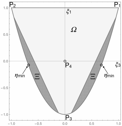
Figure 1: The lamination domain $\Omega$ for an orthotropic tensor $\mathbb{A}$ and the auxeticity domain $\Xi$ for material 2 in Table 1. The lamination points indicated by $\eta_{\min}$ give the minimum of the function $\eta(\xi_{3},\xi_{1})$ in Eq. 19.

Lamination points P${}_{1}=(1,1)$ and P${}_{2}=(-1,1)$ correspond to a laminate with all the plies at $0$ or $\frac{\pi}{2}$ respectively, the point P${}_{3}=(0,-1)$ to a balanced angle ply with orientation angles $\pm\frac{\pi}{4}$, P${}_{4}=(0,0)$ to an isotropic laminate. In addition, the lamination point of an angle-ply laminate belongs necessarily to the parabolic boundary of $\Omega$, while that of a cross-ply laminate to the line P${}_{1}-$P₂.

Miki[31] has also shown that a tensor $\mathbb{D}$ describing the bending behavior has exactly the same lamination domain, although the definition of the relevant lamination parameters is different. That is why all the results of this paper, concerning extension, can be exported identically to bending, the stacking sequence apart. We just remark the geometric meaning of a negative Poisson’s ratio for $\mathbb{D}$: the curvatures $\kappa_{1}$ and $\kappa_{2}$ due to a bending moment $M_{1}$ have the same sign, i.e. locally the deformed surface is made of elliptic points, cf. [32, 33, 34].

2.3 Auxeticity conditions for an orthotropic laminate

In [10] it has been shown that an orthotropic laminate can be auxetic for some directions if and only if

$$\min_{(\xi_{3},\xi_{1})\in\Omega}\ \eta(\xi_{3},\xi_{1})<0,$$ (18)

with

$$\eta(\xi_{3},\xi_{1}):=2(\tau_{0}\tau_{1}-\xi_{3}^{2})-\tau_{0}^{2}+\rho^{2}\xi_{1}^{2}-2|\xi_{3}^{2}-(-1)^{K}\tau_{1}\rho\ \xi_{1}|.$$ (19)

Whether or not this condition is satisfied for some lamination points, i.e. on a subset $\Xi\subset\Omega$, depends upon the material properties, i.e. on $\tau_{0},\tau_{1}$ and $(-1)^{K}\rho$. Hence, auxetic laminates can be obtained only using plies with some specific properties. The discussion of the minimum of $\eta(\xi_{3},\xi_{1})$ and hence of the auxeticity condition is rather articulated and for that the reader is addressed to [10]. Here, we just recall that the minimum of $\eta(\xi_{3},\xi_{1})$ belongs to the parabolic boundary of $\Omega$, i.e. it can be realized by angle-ply sequences, but not exclusively.

Table 1 shows the characteristics of some UD composite plies whose mechanical properties give a non empty subset $\Xi$ of $\Omega$. The subset $\Xi$ and the lamination points giving the minimum of $\eta(\xi_{3},\xi_{1})$ for material 2 in Table 1 are shown in Fig. 1.

Table 1: Some examples of UD plies. Modules are in GPa, $\varPhi_{0}=\varPhi_{1}=0\Rightarrow K=0$ for all the plies.

Mat.	$E_{1}$	$E_{2}$	$G_{12}$	$\nu_{12}$	$T_{0}$	$T_{1}$	$R_{0}$	$R_{1}$	$\tau_{0}$	$\tau_{1}$	$\rho$
1	10.00	0.42	0.75	0.24	1.66	1.34	0.91	1.20	1.383	1.116	0.758
2	181.00	10.30	7.17	0.28	26.88	24.74	19.71	21.43	1.254	1.154	0.919
3	205.00	18.50	5.59	0.23	29.80	29.14	24.21	23.42	1.272	1.244	1.033
4	86.90	5.52	2.14	0.34	12.23	12.11	10.09	10.25	1.193	1.181	0.984
5	207.00	5.00	2.60	0.25	27.52	26.85	24.93	25.29	1.088	1.062	0.986
6	76.00	5.50	2.10	0.34	10.85	10.74	8.75	8.88	1.221	1.209	0.984
7	207.00	21.00	7.00	0.30	30.67	30.35	23.67	23.46	1.307	1.293	1.009
8	134.00	7.00	4.20	0.25	19.34	18.12	15.14	15.93	1.214	1.138	0.951
9	85.00	5.60	2.10	0.34	11.98	11.89	9.88	10.00	1.198	1.189	0.988
10	294.50	6.34	4.90	0.23	39.73	38.01	34.83	36.06	1.102	1.054	0.966
11	109.70	8.55	5.31	0.30	16.89	15.53	11.58	12.73	1.327	1.220	0.910
12	131.70	8.76	5.03	0.28	19.55	18.26	14.52	15.45	1.265	1.182	0.940
13	133.10	9.31	3.74	0.34	19.02	18.74	15.28	15.60	1.219	1.201	0.979
14	135.00	9.24	6.28	0.32	20.55	18.89	14.27	15.83	1.298	1.193	0.901
15	128.00	13.00	6.40	0.30	20.00	18.77	13.60	14.51	1.378	1.293	0.937

1: Pine wood[15]	9  : Kevlar-epoxy[8]
2: Carbon-epoxy T300/5208[16]	10: Carbon-epoxy GY70/34[35]
3: Boron-epoxy B(4)-55054[16]	11: Carbon-bismaleimide AS4/5250-3[35]
4: Kevlar-epoxy 149[36]	12: Carbon-peek AS4/APC2[35]
5: Carbon-epoxy[7]	13: Carbon-epoxy AS4/3502[35]
6: Kevlar-epoxy[7]	14: Carbon-epoxy T300/976[35]
7: Boron-epoxy[7]	15: Carbon-epoxy 3 MXP251S[37]
8: Carbon-epoxy[8]

3 Minimization of $\nu_{12}(\theta)$

The first problem considered in this paper is: for a giving layer, determine the lamination point giving the laminate having the lowest Poisson’s ratio. Mathematically speaking, this amounts to solve the following constrained nonlinear optimization problem:

$$\begin{split}&\ \mathrm{given\ }\tau_{0},\tau_{1},(-1)^{K}\rho,\\ &\min_{(\xi_{3},\xi_{1})\in\Xi,\ \theta\in\left[0,\frac{\pi}{2}\right]}\nu_{12}^{A}(\theta),\end{split}$$ (20)

with $\nu_{12}^{A}(\theta)$ given by Eq. (16). Unfortunately, this minimization problem does not have a solution in an analytical form, the equations being too involved. Nevertheless, some considerations can be done analyzing what actually happens for the function $\nu_{12}^{A}(\theta)$ in the lamination domain $\Omega$. To this end, setting $\frac{d\nu_{12}^{A}(\theta)}{d\theta}=0$, some standard passages give the root

$$\cos 2\theta=-\frac{B+\sqrt{B^{2}-4C(A-C)}}{4C},$$ (21)

where

$$\begin{array}[]{c}A=\xi_{3}[\rho^{2}\xi_{1}^{2}-5\xi_{3}^{2}+3(-1)^{K}\rho\tau_{1}\xi_{1}+2\tau_{0}\tau_{1}],\vskip 12.0pt plus 4.0pt minus 4.0pt\\ B=-2[(-1)^{K}\rho\xi_{1}+\tau_{0}][(-1)^{K}\rho\tau_{1}\xi_{1}-\xi_{3}^{2}],\vskip 12.0pt plus 4.0pt minus 4.0pt\\ C=\xi_{3}[(-1)^{K}\rho\tau_{1}\xi_{1}-\xi_{3}^{2}].\end{array}$$ (22)

Injecting this root into the Eq. (16) we obtain the variation of the minimum of $\nu_{12}(\theta)$ over the lamination domain $\Omega$; the final formula giving ${\nu_{12}}_{\min}(\xi_{3},\xi_{1})$ is omitted here because too much long. However, this function is plotted in Fig. 2 for material 2 in Tab. 1, where it is apparent that the lamination point giving the minimum of ${\nu_{12}}_{\min}(\xi_{3},\xi_{1})$ is located on the parabolic boundary of $\Omega$.

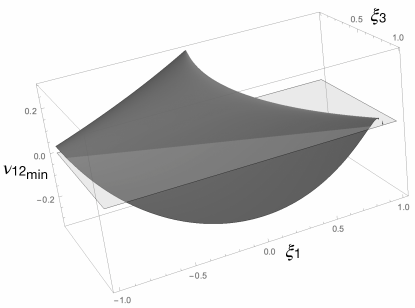
Figure 2: The function ${\nu_{12}}_{\min}(\xi_{3},\xi_{1})$ for material 2 in Tab. 1.

This situation is quite typical. In fact, an investigation made using a standard numerical search algorithm, confirms that for all the materials in Table 1 the optimal lamination point is located on the parabolic boundary of $\Omega$, see Fig. 3.

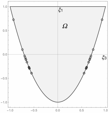
Figure 3: The lamination points giving the minimum $\nu_{12}$ for all the materials in Table 1. The points on the left side of the boundary corresponds to angle-ply laminates with the orientation angles turned of $90^{\circ}$ with respect to the orientations of the corresponding points on the right side.

An interesting consequence of these results is that for all these materials the orthotropic laminate with the minimum $\nu_{12}$ can be obtained using an angle-ply sequence. This generalizes what argued by Miki and Murotsu, [11]: two directions, namely $\pm\delta$, are sufficient to obtain, for a given UD material, the orthotropic laminate with the lowest (negative) Poisson’s ratio. Finally, we can formulate a conjecture: for any UD material, the orthotropic laminate having the most negative, i.e. with the lowest, Poisson’s ratio, can always be obtained using an angle-ply sequence. A rigorous, definitive mathematical demonstration of this conjecture remains to be done, but apparently it seems, for the while, impossible to be get.

To end this Section, in Tab. 2 the minimum value of ${\nu_{12}}_{\min}(\theta)$ for all the materials in Tab. 1 is presented, along with the coordinates $(\xi_{3},\xi_{1})$ of the lamination point and the angle $\delta$ of the corresponding angle-ply laminate. To remark that, in all the cases, $\theta<45^{\circ}$ and $\delta<30^{\circ}$.

Table 2: Minimum Poisson’s ratio for laminates composed of the materials in Table 1.

Mat.	${\nu_{12}}_{\min}$	$\theta\ (^{\circ})$	$\xi_{3}$	$\xi_{1}$	$\delta\ (^{\circ})$
1	-0.42	31.2	0.93	0.72	10.9
2	-0.33	39.1	0.68	-0.07	23.5
3	-0.23	41.9	0.55	-0.39	28.3
4	-0.35	40.2	0.60	-0.27	26.4
5	-0.95	34.2	0.69	-0.03	23.0
6	-0.28	40.9	0.59	-0.29	26.8
7	-0.16	42.7	0.55	-0.39	28.3
8	-0.39	38.6	0.67	-0.11	24.1
9	-0.33	40.4	0.60	-0.28	26.6
10	-0.94	33.1	0.74	0.10	21.0
11	-0.20	41.2	0.65	-0.16	24.8
12	-0.28	40.2	0.65	-0.16	24.8
13	-0.29	40.7	0.60	-0.27	26.5
14	-0.24	40.3	0.67	-0.10	24.0
15	-0.12	42.8	0.59	-0.29	26.8

4 Maximization of the auxetic zone

In a previous work it has been proved that a totally auxetic orthotropic laminate composed by orthotropic plies that are not auxetic themselves cannot exist, [10]. As a consequence, it is meaningful and interesting for practical applications to find the conditions that maximize the auxetic zone of such a laminate. In other words, for a given material, we look for the stacking sequence giving the laminate that has the largest set of directions where $\nu_{12}<0$.

Because $\mathbb{S}_{11}(\theta)>0\ \forall\theta,$ the sign of $\nu_{12}(\theta)$ depends uniquely on the numerator in Eq. (1) and hence, Eq. (16), $\nu_{12}^{A}(\theta)>0\iff$

$$\varPsi(\theta):=2(\tau_{0}\tau_{1}{-}\xi_{3}^{2}){-}\tau_{0}^{2}{+}\rho^{2}\xi_{1}^{2}{+}2[\xi_{3}^{2}{-}(-1)^{K}\tau_{1}\rho\xi_{1}]\cos 4\theta<0.$$ (23)

The condition of auxeticity for an orthotropic laminate is hence periodic of $\pi/2$, which means that if a material allows the fabrication of partially auxetic orthotropic laminates, [10], then there are four auxetic zones symmetric with respect to the $x_{1}$ and $x_{2}$ axes and that $\nu_{12}>0$ in correspondence of the axes, i.e. for $\theta=0,\pi/2$. In fact,

$$\varPsi(\theta)<0\ \iff\ \cos 4\theta<\lambda(\xi_{3},\xi_{1}):=\frac{\tau_{0}^{2}-\rho^{2}\xi_{1}^{2}-2(\tau_{0}\tau_{1}{-}\xi_{3}^{2})}{2[\xi_{3}^{2}-(-1)^{K}\tau_{1}\rho\xi_{1}]},$$ (24)

and because $\cos 4\theta$ is periodic of $\pi/2$, the auxetic zone, from now on denoted by $\varDelta\theta$, is necessarily symmetric with respect to $\theta=\pi/4$, see Fig. 4.

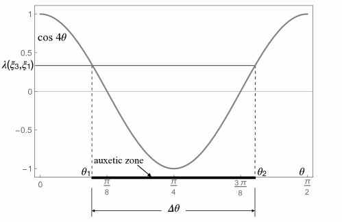
Figure 4: Symmetry of the auxetic zone.

For $\theta=0,\pi/2$ it is necessarily $\nu_{12}>0$ because, as shown in [10], totally auxetic orthotropic laminates made by identical non-auxetic orthotropic layers cannot exist.

The problem considered in this Section, i.e. the maximization of the interval $\varDelta\theta$, corresponds hence to:

$$\max_{(\xi_{3},\xi_{1})\in\Xi}\lambda(\xi_{3},\xi_{1}).$$ (25)

Unlike the case studied in the previous Section, this problem has an analytical solution. In fact, differentiating $\lambda(\xi_{3},\xi_{1})$ with respect to $\xi_{3}$ gives

$$\frac{\partial\lambda}{\partial\xi_{3}}=\xi_{3}\frac{\rho^{2}\xi_{1}^{2}-2(-1)^{K}\tau_{1}\rho\xi_{1}-\tau_{0}(\tau_{0}-2\tau_{1})}{4\left[\xi_{3}^{2}-(-1)^{K}\tau_{1}\rho\xi_{1}\right]^{2}}.$$ (26)

It is hence apparent that $\frac{\partial\lambda(0,\xi_{1})}{\partial\xi_{3}}=0$, i.e. for a given $\xi_{1}=\xi_{1}^{*}$, the function $\lambda(\xi_{3},\xi_{1}^{*})$ has a stationary point only at $\xi_{3}=0$, then it is necessarily positive or negative $\forall(\xi_{3},\xi_{1}^{*})\in\Xi$. Then, because the line $\xi_{3}=0\notin\Xi$, otherwise partially auxetic laminates could exist $\forall(\xi_{3},\xi_{1})\in\Omega$, which cannot be, see [10], along any straight line $\xi_{1}=\xi_{1}^{*}$ the maximum of $\lambda(\xi_{3},\xi_{1}^{*})$ is get for the maximum value of $\xi_{3}$, i.e. on the parabolic boundary of $\Omega$, cf. Fig. 1 (on the boundary of $\Xi,\nu_{12}=0\Rightarrow\varDelta\theta=0$). A typical example of the function $\lambda(\xi_{3},\xi_{1})$ is shown in Fig. 5 for material 2 in Tab. 1.

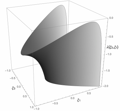
Figure 5: The function $\lambda(\xi_{3},\xi_{1})$ for material 2 in Tab. 1.

On such parabolic boundary, see Eq. (17),

$$\xi_{3}^{2}=\frac{1}{2}(\xi_{1}+1),$$ (27)

we put $\lambda(\xi_{3},\xi_{1})=\widehat{\lambda}(\xi_{1})$ with

$$\widehat{\lambda}(\xi_{1})=\frac{\tau_{0}^{2}-2\tau_{0}\tau_{1}+1+\xi_{1}-\rho^{2}\xi_{1}^{2}}{1+[1-2(-1)^{K}\tau_{1}\rho]\xi_{1}}.$$ (28)

The function $\widehat{\lambda}(\xi_{1})$ for material 2 in Tab. 1 is shown in Fig. 6.

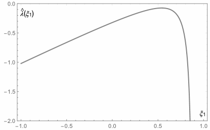
Figure 6: The function $\widehat{\lambda}(\xi_{1})$ for material 2 in Tab. 1.

Differentiating, after some standard passages, we get that $\frac{d\widehat{\lambda}}{d\xi_{1}}=0$ for

$$\xi_{1}^{opt}=\frac{\rho^{2}-\sqrt{\rho^{4}+\rho^{2}(2(-1)^{K}\rho\tau_{1}-1)[(2(-1)^{K}\rho\tau_{1}-1)(2\tau_{1}-\tau_{0})\tau_{0}-2(-1)^{K}\rho\tau_{1}]}}{\rho^{2}(2(-1)^{K}\rho\tau_{1}-1)},$$ (29)

which gives also

$$\xi_{3}^{opt}=\pm\sqrt{\frac{\xi_{1}^{opt}+1}{2}}.$$ (30)

The lamination point $(\xi_{3}^{opt},\xi_{1}^{opt})$ maximizes $\varDelta\theta$ for the given material. Because this point is on the parabolic boundary of $\Omega$, it can be realized fabricating an angle-ply laminate having orientation angles $\pm\delta$ with

$$\delta=\frac{1}{2}\arccos\xi_{3}^{opt}=\frac{1}{4}\arccos\xi_{1}^{opt}.$$ (31)

The situation depicted in Figures 5 and 6 is quite typical and in Tab. 3 the value of $\varDelta\theta$ is shown for all the materials in Tab. 1; the table is completed with the coordinates $(\xi_{3}^{opt},\xi_{1}^{opt})$ of the lamination point, the angles $\theta_{1}$ and $\theta_{2}$, bounds of the auxetic zone, see Fig. 4, the angle $\delta$ of the corresponding angle-ply laminate, the value of ${\nu_{12}}_{\min}(\theta)$ and its direction $\theta_{\min}$. To remark that, unlike the previous case, $\theta_{\min}$ can be greater than $45^{\circ}$, while in all the cases $\delta<30^{\circ}$, like before. Moreover, in the most part of cases it is $\max\lambda(\xi_{3},\xi_{1})<0\Rightarrow\varDelta\theta<\frac{\pi}{4}$, see Fig. 4. However, this cannot be generalized: for materials 1, 5 and 10, $\max\lambda(\xi_{3},\xi_{1})>0$ and $\varDelta\theta>\frac{\pi}{4}$. The lamination points giving $\varDelta\theta_{\max}$ for all the materials in Tab. 1 are shown in Fig. 7. Comparing this figure with Fig. 3, it is apparent that the lamination point giving $\varDelta\theta_{\max}$ are, generally speaking, located in a position on the boundary of $\Omega$ having a greater $\xi_{1}$ than the points giving, for the same material, the minimum of $\nu_{12}$. In practice, this means that the angle-ply giving $\varDelta\theta_{\max}$ has an orientation angle $\delta$ smaller than the one giving the minimum of $\nu_{12}$. Comparing the results in Tables 2 and 3, it can be checked that this is true for all the examined materials.

Table 3: Maximum auxetic zone for laminates composed of the materials in Table 1.

Mat.	$\xi_{3}^{opt}$	$\xi_{1}^{opt}$	$\theta_{1}\ (^{\circ})$	$\theta_{2}\ (^{\circ})$	$\varDelta\theta\ (^{\circ})$	$\delta\ (^{\circ})$	${\nu_{12}}_{\min}$	$\theta_{\min}\ (^{\circ})$
1	1.00	1.00	8.9	81.1	72.2	0.0	-0.39	27.2
2	0.88	0.54	23.6	66.4	42.8	14.3	-0.19	37.2
3	0.73	0.07	30.7	59.3	28.6	21.5	-0.16	41.1
4	0.81	0.31	26.9	63.1	36.2	18.0	-0.21	38.9
5	0.94	0.75	16.2	73.8	57.6	10.3	-0.36	30.5
6	0.78	0.22	28.6	61.4	32.7	19.3	-0.18	39.9
7	0.69	-0.04	33.0	56.9	23.9	23.1	-0.12	42.3
8	0.87	0.53	22.9	67.0	44.0	14.5	-0.21	36.6
9	0.80	0.28	27.4	62.6	35.1	18.5	-0.21	39.2
10	0.96	0.85	13.9	76.0	62.1	8.0	-0.31	28.9
11	0.81	0.31	28.3	61.7	33.3	17.9	-0.14	40.2
12	0.83	0.39	26.2	63.8	37.6	16.8	-0.17	38.8
13	0.79	0.25	28.1	61.9	33.8	18.8	-0.19	39.7
14	0.84	0.43	26.3	63.7	37.3	16.2	-0.16	39.0
15	0.72	0.03	32.9	57.1	24.1	22.1	-0.10	42.4

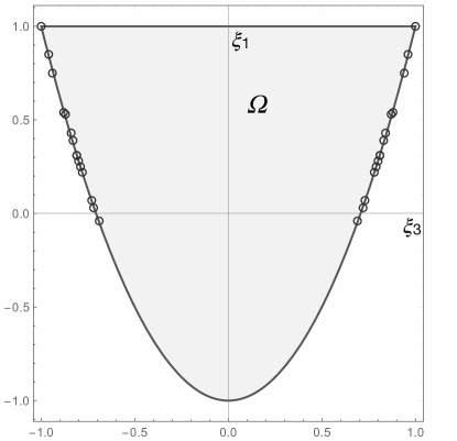
Figure 7: The lamination points giving the maximum of $\varDelta\theta$ for all the materials in Table 1. The points on the left side of the boundary corresponds to angle-ply laminates with the orientation angles turned of $90^{\circ}$ with respect to the orientations of the corresponding points on the right side.

5 Numerical examples and final considerations

For example, we consider in this Section four materials among those in Tab. 1 and present for them the maps of the lamination points, Fig. 8, and the directional diagrams of $\nu_{12}$, Fig. 9, for the laminates solution of the two problems considered above.

These four cases are quite typical of the auxeticity of laminates composed by standard composite materials. In all of these cases we can remark that the laminate with $\varDelta\theta_{\max}$ is always get using an angle ply with a smaller $\delta$ than the laminate having ${\nu_{12}}_{\min}$. The difference in the auxetic zone between these two types of laminates can be rather important. Even more different is the minimum value of the Poisson’s ratio: passing from the solution for $\varDelta\theta_{\max}$ to that for ${\nu_{12}}_{\min}$, the value of $\nu_{12}$ passes from $-0.19$ to $-0.33$ for material 2, from $-0.36$ to $-0.95$ for material 5, from $-0.21$ to $-0.39$ for material 8 and from $-0.31$ to $-0.94$ for material 10. Theses data show perfectly that the laminates solution of the two different problems have, for the same constituent material, very different auxetic properties.

To conclude, we recall that angle-ply stacks can always be used to obtain auxetic laminates, although this is not compulsory, and remark that the auxetic properties of the laminates are rather sensitive to the orientation angle $\delta$ of the angle-ply sequence: a small change of $\delta$ can change substantially the auxeticity of the laminate.

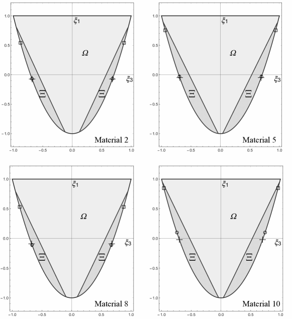
Figure 8: The case of four materials in Tab. 1: for each material, the domain $\Xi\subset\Omega$ giving partially auxetic laminates is indicated, along with the lamination points corresponding to the laminates with $\eta_{\min},{\nu_{12}}_{\min},\varDelta\theta_{\max}$, denoted respectively by $\circ,+$ and $\square$.

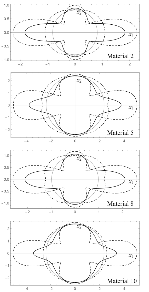
Figure 9: The directional diagrams of $\nu_{12}$ for four materials in Tab. 1: for each material, the curves representing $\nu_{12}$ of the single layer and of the laminates with ${\nu_{12}}_{\min}$ and $\varDelta\theta_{\max}$ are shown, denoted respectively by a dot-dashed, a dashed and a solid line. The thin circle marks the zero value: inside it, $\nu_{12}$ is negative.

References

- [1] Cho H, Seo D and Kim DN. Mechanics of auxetic materials. In Schmauder S and Chen CS (eds.) Handbook of mechanics of materials. Singapore: Springer, 2019. pp. 733–757.
- [2] Love AEH. A treatise on the mathematical theory of elasticity. New York, NY: Dover, 1944.
- [3] Sokolnikoff IS. Mathematical theory of elasticity. New York, NY: McGraw-Hill, 1946.
- [4] Gurtin ME. An introduction to continuum mechanics. New York, NY: Academic Press Inc., 1981.
- [5] Prawoto Y. Seeing auxetic materials from the mechanics point of view: A structural review on the negative Poisson’s ratio. Computational Materials Science 2012; 58: 140–153.
- [6] Shukla S and Behera BK. Auxetic fibrous structures and their composites: A review. Composite Structures 2022; 290(115530).
- [7] Jones RM. Mechanics of composite materials. Second Edition. Philadelphia, PA: Taylor & Francis, 1999.
- [8] Gay D. Composite Materials Design and Applications - Third Edition. Boca Raton, FL: CRC Press, 2014.
- [9] Vasiliev VV and Morozov EV. Mechanics and analysis of composite materials. Elsevier, 2001.
- [10] Vannucci P. Anisotropic auxetic composite laminates: a polar approach. Journal of Composite Materials 2024; URL https://doi.org/10.1177/00219983241256335.
- [11] Miki M and Murotsu Y. The peculiar behavior of the Poisson’s ratio of laminated fibrous composites. JSME International Journal 1989; 32(1): 67–72.
- [12] Zhang R, Yeh HL and Yeh HY. A preliminary study of negative Poisson’s ratio of laminated fiber reinforced composites. Journal of Reinforced Plastics and Composites 1998; 17(18): 1651–1664.
- [13] Verchery G. Les invariants des tenseurs d’ordre 4 du type de l’élasticité. In Proc. of Colloque Euromech 115 (Villard-de-Lans, 1979): Comportement mécanique des matériaux anisotropes. Paris: Editions du CNRS, 1982. pp. 93–104.
- [14] Vannucci P. Strange laminates. Mathematical Methods in the Applied Sciences 2012; 35: 1532–1546.
- [15] Lekhnitskii SG. Theory of elasticity of an anisotropic elastic body. San Francisco, CA: English translation (1963) by P. Fern, Holden-Day, 1950.
- [16] Tsai SW and Hahn T. Introduction to composite materials. Stamford, CT: Technomic, 1980.
- [17] Ting TCT. Anisotropic elasticity. Oxford, UK: Oxford University Press, 1996.
- [18] Vannucci P. Plane anisotropy by the polar method. Meccanica 2005; 40: 437–454.
- [19] Vannucci P. Anisotropic elasticity. Berlin, Germany: Springer, 2018.
- [20] Vannucci P. A special planar orthotropic material. Journal of Elasticity 2002; 67: 81–96.
- [21] Vincenti A, Verchery G and Vannucci P. Anisotropy and symmetries for elastic properties of laminates reinforced by balanced fabrics. Composites Part A 2001; 32: 1525–1532.
- [22] Vannucci P. On bending-tension coupling of laminates. Journal of Elasticity 2001; 64: 13–28.
- [23] Vannucci P. On the mechanical and mathematical properties of the stiffness and compliance coupling tensors of composite anisotropic laminates. Journal of Composite Materials 2023; 57(26): 4197–4214.
- [24] Vannucci P. On the thermoelastic coupling of anisotropic laminates. Archive of Applied Mechanics 2024; 94: 1121–1149.
- [25] Vannucci P and Verchery G. Stiffness design of laminates using the polar method. International Journal of Solids and Structures 2001; 38: 9281–9294.
- [26] Vannucci P and Verchery G. A special class of uncoupled and quasi-homogeneous laminates. Composites Science and Technology 2001; 61: 1465–1473.
- [27] Tsai SW and Pagano NJ. Invariant properties of composite materials. In Tsai SW, Halpin JC and Pagano NJ (eds.) Composite Materials Workshop. Stamford, CT: Technomic, 1968.
- [28] Vannucci P. A note on the elastic and geometric bounds for composite laminates. Journal of Elasticity 2013; 112: 199–215.
- [29] Miki M. Material design of composite laminates with required in-plane elastic properties. In Proc. of ICCM 4 - Fourth International Conference on Composite Materials. Tokio, Japan, 1982. pp. 1725–1731.
- [30] Miki M. A graphical method for designing fibrous laminated composites with required in-plane stiffness. Transactions of the Japanese Society of Composite Materials 1983; 9: 51–55.
- [31] Miki M. Design of laminated fibrous composite plates with required flexural stiffness. In Vinson JR and Taya M (eds.) Recent advances in composites in the USA and Japan - ASTM STP 864. Philadelphia, PA: American Society for Testing and Materials, pp. 387–400.
- [32] Toponogov VA. Differential geometry of curves and surfaces - A concise guide. Birkhäuser, 2006.
- [33] Pressley A. Elementary differential geometry. Berlin: Springer, 2010.
- [34] Vannucci P. Tensor algebra and analysis for engineers - With applications to differential geometry of curves and surfaces. Singapore: World Scientific, 2023.
- [35] AAVV. MIL-HDBK - Composite Materials Handbook - Volume 2. Technical report, US Department of Defense, 2002.
- [36] Daniel IM and Ishai O. Engineering mechanics of composite materials. Oxford, UK: Oxford University Press, 1994.
- [37] Gürdal Z, Haftka RT and Hajela P. Design and optimization of laminated composite materials. New York, NY: J. Wiley & Sons, 1999.