Schrödinger Unitary Cellular Automata

Abstract

We propose a class of cellular automata for the Hamiltonian of a free particle. It is based on a two-step unitary evolution operator in discrete time and space. Various experiments with one and two-dimensional cellular automata are used to analyze 1) phase velocities of plane waves, 2) dispersion and group velocities of wavepackets, 3) energy levels of infinite potential wells and harmonic oscillators, and 4) interference from double-slit diffraction. Some of the differences between their known (analytical) results and the cellular-automata approximations are intriguing.

Keywords: Schrödinger equation, cellular automata, double-slit experiment.

1 Introduction

The Schrödinger equation is a linear partial differential equation that governs the wave function of a quantum-mechanical system. The one-dimensional Schrödinger equation for a single particle has the form

$$i\hbar\frac{\partial\Psi(x,t)}{\partial t}=-\frac{\hbar^{2}}{2m}\frac{\partial^{2}\Psi(x,t)}{\partial x^{2}}+V(x)\Psi(x,t)~{},$$ (1.1)

where $\Psi(x,t)$ is the wave function, $\hbar$ the Planck constant, $m$ the particle’s mass, and $V(x)$ a potential-energy function. Textbooks such as [1] present analytical solutions for a variety of simple quantum systems. For systems with non-trivial V(x) or irregular boundary conditions, numerical techniques can be used to approximate the continuous solution of $\Psi$ in discrete time and space. This paper explores the opposite perspective: what if the Schrödinger equation is a continuous approximation of a discrete universe? What if, e.g. at the Planck scale, quantum dynamics occurs on a discrete lattice and in discrete time steps, as for example in [2, 3]? For this exploration cellular automata are used as a tool.

The Schrödinger equation can be solved using numerical techniques, such as the Crank-Nicolson method [4]. Mena [5], amongst others, applied this method to various systems, including the double-slit experiment. Let $\Psi(t)$ denote the wave function at time $t$. Cranck-Nicolson relates the evolved state $\Psi(t+\Delta t)$ over an incremental time step $\Delta t$ to the previous state by

$$\Psi(t+\Delta t)~{}=~{}(\mathbf{M}^{-1}\mathbf{A})\Psi(t)~{}=~{}\mathbf{U}\;\Psi(t)~{},$$ (1.2)

where matrices $\mathbf{M}$ and $\mathbf{A}$ represent the forward Euler and backward Euler integration steps. Evolution matrix $\mathbf{U}=\mathbf{M}^{-1}\mathbf{A}$ is an approximately unitary $N\!\times\!N$ matrix, where $N$ is the number cells, of a possibly multi-dimensional grid. Crucially, matrix $\mathbf{U}$ is dense: all its elements are nonzero. This non-locality is not surprising, as the Schrödinger equation is non-relativistic: the probability of finding a particle arbitrarily far away from the initial region is nonzero for any $\Delta t>0$. This non-local approximation of the Schrödinger equation is therefore not suitable for a cellular automaton.

Quoting [6]:

Cellular automata are discrete dynamical systems whose behavior is completely specified in terms of a local relation, much as is the case for a large class of continuous dynamical systems defined by partial differential equations. In this sense, cellular automata are the computer scientist’s counterpart to the physicist’s concept of “field.”

Our cellular automata consist of a finite number, $N$, of cells, where the state of each cell is a complex number representing the value of the wave function at that location. The “local relation” (update rule) in the quote above can be represented by an $N\!\times\!N$ evolution matrix $\mathbf{U}$. For a one-dimensional cellular automaton $\mathbf{U}$ must be both unitary, to preserve Born probability, and band-structured, to meet the locality requirement of CA. These cellular automata are known as unitary cellular automata (UCA) [7] and early work along these lines includes [8]. UCA form a special case of quantum cellular automata (QCA) [9, 10], where the state of each cell typically comprises one or a few qubits.

The contributions of this work include the following.

• An approximate evolution matrix $\mathbf{U}$ for the Schrödinger Hamiltonian that is both unitary (as required by quantum mechanics), and band structured (as required for cellular automata).

• A systematic exploration of the physical properties of these automata, including phase and group velocities, dispersion, energy levels, diffraction, and interference.

• A two-dimensional Schrödinger UCA describing the double-slit experiment.

2 Schrödinger Cellular Automata

2.1 A discrete Schrödinger Hamiltonian

For a one-dimensional cellular automaton with cell size $a$, a discrete-space version of the Schrödinger equation 1.1 becomes

$$i\hbar\frac{\partial\Psi(x,t)}{\partial t}=-\frac{\hbar^{2}}{2m}\frac{1}{a^{2}}\big{(}\Psi(x\!+\!1,t)-2\Psi(x,t)+\Psi(x\!-\!1,t)\big{)}+V(x)\Psi(x,t)~{},$$ (2.1)

where spatial coordinate $x$ is now integer valued. For now, $V(x)$ is assumed to be zero. (Nonzero $V(x)$ will be revisited in Subsection 2.3.) In matrix form (2.1) then becomes:

$$i\hbar\frac{\partial\Psi(x,t)}{\partial t}=\mathbf{H}\Psi(x,t)~{}.$$ (2.2)

Hamiltonian $\mathbf{H}$, assuming periodic boundary conditions, can be represented by a two-dimensional circulant matrix. For $N\!=\!8$ cells

$$\mathbf{H}=\delta\hat{\mathbf{H}},~{}~{}~{}~{}\mathrm{where}~{}~{}~{}~{}~{}\delta=\frac{\hbar^{2}}{2m}\frac{1}{a^{2}}~{},~{}~{}~{}~{}\hat{\mathbf{H}}=\left[\begin{matrix}2&-1&0&0&0&0&0&-1\\ -1&2&-1&0&0&0&0&0\\ 0&-1&2&-1&0&0&0&0\\ 0&0&-1&2&-1&0&0&0\\ 0&0&0&-1&2&-1&0&0\\ 0&0&0&0&-1&2&-1&0\\ 0&0&0&0&0&-1&2&-1\\ -1&0&0&0&0&0&-1&2\end{matrix}\right].$$ (2.3)

The time evolution of a system is commonly described by

$$\mid\!{\Psi(t)}\rangle\;=\;\mathbf{U}(t)\mid\!{\Psi(0)}\rangle~{},~{}~{}~{}~{}~{}\mathrm{with}~{}~{}~{}~{}~{}\mathbf{U}(t)=\exp{\big{(}{-i\frac{1}{\hbar}\mathbf{H}t}\big{)}}$$ (2.4)

The discrete-time evolution for integer time $t$, $0\leq t$ and fixed time step $\tau$, thus becomes

$$\mid\!{\Psi((t+1)\tau)}\rangle\;=\;\mathbf{U}\mid\!{\Psi(t\tau)}\rangle~{},$$ (2.5)

where

$$\mathbf{U}=\exp{\big{(}{-i\frac{\tau}{\hbar}\mathbf{H}}\big{)}}=\exp{\big{(}{-i\theta\hat{\mathbf{H}}}\big{)}}~{},~{}~{}~{}~{}~{}\mathrm{with}~{}~{}~{}~{}~{}\theta=\frac{\tau}{\hbar}\delta=\frac{\hbar}{2m}\frac{\tau}{a^{2}}~{}.$$ (2.6)

Constant $\theta$ is dimensionless, and can be seen as a rotation angle. Matrix $\mathbf{U}$ is a dense matrix: all its elements are nonzero. It is not a band matrix, and therefore it is not usable to describe a cellular automaton. The probability of finding the particle in cell $x$ at time $t$, denoted by $P(x,t)$, is given by Born’s rule:

$$P(x,t)\;=\;\mid\!{\Psi(x,t)}\!\mid^{2}~{},\hskip 85.35826ptP(t)=\sum_{x}P(x,t)=1~{}.$$ (2.7)

Matrix $\hat{\mathbf{H}}$ can be rewritten as

$$\hat{\mathbf{H}}=2\mathbf{I}+\overline{\mathbf{H}}~{},$$ (2.8)

where $\mathbf{I}$ is the identity matrix of the same dimensions as $\hat{\mathbf{H}}$, and $\overline{\mathbf{H}}$ equals $\hat{\mathbf{H}}$ stripped of its diagonal. Since commutator $[\overline{\mathbf{H}},\mathbf{I}]=0$,

$$\exp{\big{(}{-i\theta\hat{\mathbf{H}}}\big{)}}~{}=~{}\exp{\big{(}{-i\theta(2\mathbf{I}+\overline{\mathbf{H}})}\big{)}}~{}=~{}\exp{\big{(}{-2i\theta}\big{)}}\exp{\big{(}{-i\theta\overline{\mathbf{H}}}\big{)}}~{}.$$ (2.9)

For the purpose of computing $P(x,t)$ it is sufficient to use $\exp{\big{(}{-i\theta\overline{\mathbf{H}}}\big{)}}$ as evolution matrix, because the fixed phase rotation over $-2\theta$ has no effect on the probability density.

For real-valued $\delta$, $\delta\overline{\mathbf{H}}$ is the same Hamiltonian as used by Grössing and Zeilinger [8] in their study of quantum cellular automata. They approximate the unitary evolution operator $\mathbf{U}$ by using only the first-order term of its expansion

$$\mathbf{U}~{}~{}=~{}~{}\exp{\big{(}{-\frac{i}{\hbar}\delta\overline{\mathbf{H}}\tau}\big{)}}~{}~{}\approx~{}~{}\mathbf{I}\!-\!\frac{i}{\hbar}\delta\overline{\mathbf{H}}\tau~{}~{}=~{}~{}\mathbf{I}\!-\!i\theta\overline{\mathbf{H}}~{}.$$ (2.10)

Matrix $\mathbf{U}$ is a three-band matrix, which nicely agrees with the locality requirement for a cellular automaton: the value of $\Psi(x,t\!+\!1)$ only depends on $\Psi(u,t)$, with $u$ an element of the local neighborhood of $x$, that is, $u\in\{x\!-\!1,x,x\!+\!1\}$. This locality comes at a price: matrix $\mathbf{U}$ is not unitary, and the overall probability $P(t)$ is therefore not preserved. In practice, this implies the need for an ad-hoc scale factor and regular normalization.

2.2 Split evolution

Next we derive an evolution matrix $\mathbf{U}$ that is both unitary (as required by quantum mechanics), and band structured (as required for cellular automata). As a first step, Hamiltonian $\hat{\mathbf{H}}$ is split into two 2$\times$2-block diagonal matrices $\hat{\mathbf{H}}_{0}$ and $\hat{\mathbf{H}}_{1}$, such that $\hat{\mathbf{H}}=\hat{\mathbf{H}}_{0}+\hat{\mathbf{H}}_{1}$, where

$$\hat{\mathbf{H}}_{0}=\mathbf{I}_{m}\otimes\mathbf{B}~{},\hskip 56.9055pt\mathbf{B}=\left[\begin{matrix}1&-1\\ -1&1\end{matrix}\right]~{},\hskip 56.9055pt\hat{\mathbf{H}}_{1}=\mathbf{S}^{-1}\hat{\mathbf{H}}_{0}\;\mathbf{S}~{}.$$ (2.11)

Here $\otimes$ denotes the Kronecker matrix product, integer $m$ satisfies $2m\!=\!N$, and matrix $\mathbf{S}$ is the so-called circular shift matrix. The matrix product $\mathbf{S}$ $\mathbf{A}$ yields a specific permutation of matrix $\mathbf{A}$, with all rows of $\mathbf{A}$ shifted down by one row and with the last row moved to the first position. Below the result of this split for $N\!=\!8$ cells.

$$\hat{\mathbf{H}}_{0}\!=\!\!\left[\begin{matrix}1&-1&0&0&0&0&0&0\\ -1&1&0&0&0&0&0&0\\ 0&0&1&-1&0&0&0&0\\ 0&0&-1&1&0&0&0&0\\ 0&0&0&0&1&-1&0&0\\ 0&0&0&0&-1&1&0&0\\ 0&0&0&0&0&0&1&-1\\ 0&0&0&0&0&0&-1&1\end{matrix}\right]\hat{\mathbf{H}}_{1}\!=\!\!\left[\begin{matrix}1&0&0&0&0&0&0&-1\\ 0&1&-1&0&0&0&0&0\\ 0&-1&1&0&0&0&0&0\\ 0&0&0&1&-1&0&0&0\\ 0&0&0&-1&1&0&0&0\\ 0&0&0&0&0&1&-1&0\\ 0&0&0&0&0&-1&1&0\\ -1&0&0&0&0&0&0&1\end{matrix}\right].$$ (2.12)

The corresponding evolution operators $\mathbf{U}_{0}$ and $\mathbf{U}_{1}$ are

$$\mathbf{U}_{0}=\exp{\big{(}{-i\theta\hat{\mathbf{H}}_{0}}\big{)}}~{},\hskip 85.35826pt\mathbf{U}_{1}=\exp{\big{(}{-i\theta\hat{\mathbf{H}}_{1}}\big{)}}~{},$$ (2.13)

with $\mathbf{U}_{1}=\mathbf{S}^{-1}\mathbf{U}_{0}\;\mathbf{S}$. Matrices $\mathbf{U}_{0}$ and $\mathbf{U}_{1}$ are both unitary and have a three-diagonal structure. For $N\!=\!8$ matrix $\mathbf{U}_{1}$ is shown below.

$$\begin{array}[]{ll}\mathbf{U}_{1}=\exp{\big{(}{-i\theta}\big{)}}\times\\ \vspace{1mm}\left[\begin{matrix}\cos{\left(\theta\right)}&0&0&0&0&0&0&i\sin{\left(\theta\right)}\\ 0&\cos{\left(\theta\right)}&i\sin{\left(\theta\right)}&0&0&0&0&0\\ 0&i\sin{\left(\theta\right)}&\cos{\left(\theta\right)}&0&0&0&0&0\\ 0&0&0&\cos{\left(\theta\right)}&i\sin{\left(\theta\right)}&0&0&0\\ 0&0&0&i\sin{\left(\theta\right)}&\cos{\left(\theta\right)}&0&0&0\\ 0&0&0&0&0&\cos{\left(\theta\right)}&i\sin{\left(\theta\right)}&0\\ 0&0&0&0&0&i\sin{\left(\theta\right)}&\cos{\left(\theta\right)}&0\\ i\sin{\left(\theta\right)}&0&0&0&0&0&0&\cos{\left(\theta\right)}\end{matrix}\right]\end{array}$$ (2.14)

Note that $\mathbf{U}_{1}$ is written in the form $\;\exp{\big{(}{-i\theta}\big{)}}\times\exp{\big{(}{-i\theta(\hat{\mathbf{H}}_{1}-\mathbf{I})}\big{)}}.$ Also matrix $\mathbf{U}_{1}\mathbf{U}_{0}$ is strictly unitary and has a five-diagonal structure, unlike matrix $\mathbf{M}^{-1}\mathbf{A}$ in Equation 1.2 used for numerical simulations [5]. For $N\!=\!8$ matrix $\mathbf{U}_{1}\mathbf{U}_{0}$ becomes

$$\begin{array}[]{ll}\mathbf{U}_{1}\mathbf{U}_{0}=\exp{\big{(}{-2i\theta}\big{)}}\times\\ \vspace{1mm}\left[\begin{matrix}\cos^{2}{\left(\theta\right)}&\frac{i\sin{\left(2\theta\right)}}{2}&0&0&0&0&-\sin^{2}{\left(\theta\right)}&\frac{i\sin{\left(2\theta\right)}}{2}\\ \frac{i\sin{\left(2\theta\right)}}{2}&\cos^{2}{\left(\theta\right)}&\frac{i\sin{\left(2\theta\right)}}{2}&-\sin^{2}{\left(\theta\right)}&0&0&0&0\\ -\sin^{2}{\left(\theta\right)}&\frac{i\sin{\left(2\theta\right)}}{2}&\cos^{2}{\left(\theta\right)}&\frac{i\sin{\left(2\theta\right)}}{2}&0&0&0&0\\ 0&0&\frac{i\sin{\left(2\theta\right)}}{2}&\cos^{2}{\left(\theta\right)}&\frac{i\sin{\left(2\theta\right)}}{2}&-\sin^{2}{\left(\theta\right)}&0&0\\ 0&0&-\sin^{2}{\left(\theta\right)}&\frac{i\sin{\left(2\theta\right)}}{2}&\cos^{2}{\left(\theta\right)}&\frac{i\sin{\left(2\theta\right)}}{2}&0&0\\ 0&0&0&0&\frac{i\sin{\left(2\theta\right)}}{2}&\cos^{2}{\left(\theta\right)}&\frac{i\sin{\left(2\theta\right)}}{2}&-\sin^{2}{\left(\theta\right)}\\ 0&0&0&0&-\sin^{2}{\left(\theta\right)}&\frac{i\sin{\left(2\theta\right)}}{2}&\cos^{2}{\left(\theta\right)}&\frac{i\sin{\left(2\theta\right)}}{2}\\ \frac{i\sin{\left(2\theta\right)}}{2}&-\sin^{2}{\left(\theta\right)}&0&0&0&0&\frac{i\sin{\left(2\theta\right)}}{2}&\cos^{2}{\left(\theta\right)}\end{matrix}\right]\end{array}$$ (2.15)

Matrix $\mathbf{U}_{1}\mathbf{U}_{0}$ also is an approximation of $\exp{\big{(}{-i\theta\hat{\mathbf{H}}}\big{)}}$:

$$\begin{array}[]{lll}\exp{\big{(}{-i\theta\hat{\mathbf{H}}}\big{)}}&=&\exp{\big{(}{-i\theta(\hat{\mathbf{H}}_{0}+\hat{\mathbf{H}}_{1})}\big{)}}\\ &=&\exp{\big{(}{-i\theta\hat{\mathbf{H}}_{1}}\big{)}}\exp{\big{(}{-i\theta\hat{\mathbf{H}}_{0}}\big{)}}+\mathcal{O}(\theta^{2})\\ &=&\mathbf{U}_{1}\mathbf{U}_{0}+\mathcal{O}(\theta^{2})~{}.\end{array}$$ (2.16)

The approximation error can be made arbitrarily small by choosing a small value for $\theta$ (i.e. a small time step $\tau$). This approximation can be improved by [11]

$$\begin{array}[]{lll}\exp{\big{(}{-i\theta\hat{\mathbf{H}}}\big{)}}=\exp{\big{(}{-i\frac{\theta}{2}\hat{\mathbf{H}}_{0}}\big{)}}\exp{\big{(}{-i\theta\hat{\mathbf{H}}_{1}}\big{)}}\exp{\big{(}{-i\frac{\theta}{2}\hat{\mathbf{H}}_{0}}\big{)}}+\mathcal{O}(\theta^{3})~{},\end{array}$$ (2.17)

which is applied in the experiments later on. By taking higher-order terms of the expansion of $\exp{(-i\theta(\hat{\mathbf{H}}_{0}+\hat{\mathbf{H}}_{1}))}$ into account, this error can be reduced further [11]. In turn, evolution operator $\mathbf{U}_{1}\mathbf{U}_{0}$ specifies Hamiltonian $\theta\hat{\mathbf{H}}_{10}$

$$\hat{\mathbf{H}}_{10}=i\frac{1}{\theta}\log\big{[}\exp{\big{(}{-i\theta\hat{\mathbf{H}}_{1}}\big{)}}\exp{\big{(}{-i\theta\hat{\mathbf{H}}_{0}}\big{)}}\big{]}~{}.$$ (2.18)

Matrix $\hat{\mathbf{H}}_{10}$ can be approximated, where the higher-order terms of the expansion appear to fill the entire matrix.

The pair of matrices $\mathbf{U}_{0}$ and $\mathbf{U}_{1}$ suggests a more fine-grained cellular evolution of the original Hamiltonian, by alternatingly applying $\mathbf{U}_{0}$ and $\mathbf{U}_{1}$ to the quantum state $\Psi(x)$. An even-numbered cell interacts alternatingly with its right-hand side and left-hand side neighbors. For odd-numbered cells the order of interaction is opposite. The cell-update rules of $\mathbf{U}_{1}\mathbf{U}_{0}$ have a bounded neighborhood, including both immediate neighbors and one of the neighbors at distance two.

The split evolution of Definition 2.11 can be generalized to an $M$-way split $\hat{\mathbf{H}}=\hat{\mathbf{H}}_{0}+\hat{\mathbf{H}}_{1}+\ldots+\hat{\mathbf{H}}_{M-1}$, such that $\hat{\mathbf{H}}_{(i+1)\!\!\mod M}=\mathbf{S}^{-1}\hat{\mathbf{H}}_{i}\;\mathbf{S}$. The corresponding blocks $\mathbf{B}$ are $M\!\times\!M$ matrices, and $\mathbf{U}_{i}$ are also (wider) band matrices. The cellular automata based on split evolution of the Hamiltonian are examples of so-called partitioning cellular automata ([6], pp 119-120), also known as block cellular automata. The $N$ cells are partitioned in two ways, each having a matching block rule, viz. $\mathbf{U}_{0}$ and $\mathbf{U}_{1}$, applied alternatingly. A partitioning cellular automaton is reversible if all of the block rules are reversible. Clearly, $\mathbf{U}_{0}$, $\mathbf{U}_{1}$, and $\mathbf{U}_{1}\mathbf{U}_{0}$ are reversible, since they are unitary.

2.3 The potential energy function $V(x)$

The discrete Schrödinger Equation 2.1 includes a position-dependent potential-energy function $V(x)$. This potential can be included in the Hamiltonian matrix as in

$$\begin{array}[]{lll}\hat{\mathbf{V}}&=&{\rm diag}\big{(}\frac{1}{\delta}V(x)\big{)}\vspace{2mm}\\ \hat{\mathbf{H}}^{\prime}&=&\hat{\mathbf{H}}+\hat{\mathbf{V}}\\ &=&(\hat{\mathbf{H}}_{0}+\hat{\mathbf{V}}_{0})+(\hat{\mathbf{H}}_{1}+\hat{\mathbf{V}}_{1})~{},\end{array}$$ (2.19)

where the potential $\hat{\mathbf{V}}$ is split over its even and odd terms. Matrices $\hat{\mathbf{H}}$ and $\hat{\mathbf{V}}$ generally do not commute and hence

$$\exp{(-i\theta(\hat{\mathbf{H}}+\hat{\mathbf{V}}))}~{}\neq~{}\exp{(-i\theta\hat{\mathbf{H}})}\exp{(-i\theta\hat{\mathbf{V}})}~{}.$$ (2.20)

The equality only holds when $\hat{\mathbf{V}}$ is a multiple of the identity matrix, equivalent to adding a fixed potential energy $V$ to all cells. The resulting rotation $\exp{(-i\theta\frac{1}{\delta}V)}$ is periodic in $V$ with period $2\pi\delta/\theta$. A non-uniform $V(x)$ results in an inhomogeneous CA and is used for the refraction experiment of Figure 10 and for the harmonic oscillator of Figure 11.

The potential energy $V(x)$ only contributes to the diagonal of the Hamiltonian. It can be shown that no real-valued $V(x)$ can cancel the off-diagonal nonzeros of matrix $\mathbf{U}_{1}\mathbf{U}_{0}$ in Identity 2.15. Hence $V(x)$ can not be used to remove the periodic boundary conditions.

2.4 Hard boundaries

The Hamiltonian matrices of Identities 2.11 can be rewritten as

$$\begin{array}[]{lll}\theta\;\hat{\mathbf{H}}_{0}&=&~{}~{}~{}~{}~{}{\rm diag}(\theta\mathbf{B},\;\theta\mathbf{B},\;\theta\mathbf{B},\ldots,\;\theta\mathbf{B})\\ \theta\;\hat{\mathbf{H}}_{1}&=&\mathbf{S}^{-1}{\rm diag}(\theta\mathbf{B},\;\theta\mathbf{B},\;\theta\mathbf{B},\ldots,\;\theta\mathbf{B})\;\mathbf{S}\end{array}\hskip 56.9055pt\mathbf{B}=\left[\begin{matrix}1&-1\\ -1&1\end{matrix}\right]~{}.$$ (2.21)

The diagonal block matrices $\theta\mathbf{B}$ are identical, leading to the periodic boundary condition of Identity 2.15. This periodic boundary condition can be removed by replacing the last $\theta\mathbf{B}$ in $\theta\hat{\mathbf{H}}_{1}$ by $\pi\mathbf{B}^{\prime}$, where

$$\mathbf{B}^{\prime}=\left[\begin{matrix}0&1\\ 1&0\end{matrix}\right]~{},\hskip 56.9055pt\mathbf{U^{\prime}}=\exp{(-i\pi\mathbf{B}^{\prime})}=\left[\begin{matrix}-1&0\\ 0&-1\end{matrix}\right]~{}.$$ (2.22)

For $N\!=\!8$ this results in

$$\begin{array}[]{ll}\theta\;\hat{\mathbf{H}}_{1}=\left[\begin{matrix}0&0&0&0&0&0&0&\pi\\ 0&-\theta&\theta&0&0&0&0&0\\ 0&\theta&-\theta&0&0&0&0&0\\ 0&0&0&-\theta&\theta&0&0&0\\ 0&0&0&\theta&-\theta&0&0&0\\ 0&0&0&0&0&-\theta&\theta&0\\ 0&0&0&0&0&\theta&-\theta&0\\ \pi&0&0&0&0&0&0&0\end{matrix}\right]~{}.\end{array}$$ (2.23)

The corresponding evolution matrix $\mathbf{U}_{1}$ is given by

$$\begin{array}[]{ll}\mathbf{U}_{1}=\exp{\big{(}{-i\theta}\big{)}}\times\\ \vspace{1mm}\left[\begin{matrix}-e^{i\theta}&0&0&0&0&0&0&0\\ 0&\cos{\left(\theta\right)}&i\sin{\left(\theta\right)}&0&0&0&0&0\\ 0&i\sin{\left(\theta\right)}&\cos{\left(\theta\right)}&0&0&0&0&0\\ 0&0&0&\cos{\left(\theta\right)}&i\sin{\left(\theta\right)}&0&0&0\\ 0&0&0&i\sin{\left(\theta\right)}&\cos{\left(\theta\right)}&0&0&0\\ 0&0&0&0&0&\cos{\left(\theta\right)}&i\sin{\left(\theta\right)}&0\\ 0&0&0&0&0&i\sin{\left(\theta\right)}&\cos{\left(\theta\right)}&0\\ 0&0&0&0&0&0&0&-e^{i\theta}\end{matrix}\right]~{}.\end{array}$$ (2.24)

Crucially, unlike in Identity 2.14, $\mathbf{U}_{1}[0,7]=\mathbf{U}_{1}[7,0]=0$: matrix $\mathbf{U}_{1}$ is not circulant, and the corresponding cellular automaton $\mathbf{U}_{1}\mathbf{U}_{0}$ has no periodic boundaries, but a hard boundary at position $N\!-\!1$. Any of the blocks $\theta\mathbf{B}$ in Identity 2.21 can be replaced by $\pi\mathbf{B}^{\prime}$, implying hard boundaries at the respective positions. Such hard boundaries are used to describe an infinite potential well in Subsections 3.3 and 3.4, as well as the screen of the double-slit experiment in Subsection 4.2.

2.5 Two-dimensional Schrödinger cellular automata

A two-dimensional Schrödinger cellular automaton operates on a 2D wave function $\Psi$ represented by a 2D matrix. Let unitary evolution matrices $\mathbf{U}_{H}$ and $\mathbf{U}_{V}$ denote two homogeneous one-dimensional CA, comprising $N_{H}$ and $N_{V}$ cells respectively. Furthermore, let $\mathbf{U}_{H}$ and $\mathbf{U}_{V}$ refer to the same particle (mass $m$), and to the same cell size $a$ and time step $\tau$. Then the Kronecker product $\mathbf{U}_{H}\otimes\mathbf{U}_{V}$ defines a homogeneous two-dimensional cellular automaton according to

$${\rm vec}\big{(}\Psi(t\!+\!\tau)\big{)}=(\mathbf{U}_{H}\otimes\mathbf{U}_{V})\;{\rm vec}\big{(}\Psi(t)\big{)}~{}.$$ (2.25)

Here ${\rm vec}(A)$ denotes the standard vectorization of matrix $A$, obtained by stacking the columns of the $A$ on top of one another. The relation between $\mathbf{U}_{H}\otimes\mathbf{U}_{V}$ and the 2D Schrödinger equation can be appreciated by means of some rewriting. First,

$$\big{(}\mathbf{U}_{H}\otimes\mathbf{U}_{V}\big{)}\;{\rm vec}\big{(}\Psi(t)\big{)}={\rm vec}{\big{(}\mathbf{U}_{V}\;\Psi(t)\;\mathbf{U}_{H}^{\top}\big{)}}~{}.$$ (2.26)

Next, $\mathbf{U}_{H}$ and $\mathbf{U}_{V}$ are expressed in terms of $\hat{\mathbf{H}}$ (Definition 2.3), by using only the first-order term of its expansion.

$$\begin{array}[]{lll}\Psi(t+\tau)&=&\mathbf{U}_{V}\;\Psi(t)\;\mathbf{U}_{H}^{\top}\vspace{1mm}\\ &=&(\mathbf{I}-i\theta\hat{\mathbf{H}}_{V})\;\Psi(t)\;(\mathbf{I}-i\theta\hat{\mathbf{H}}_{H})^{\top}+\mathcal{O}(\theta^{2})\vspace{1mm}\\ &=&\Psi(t)-i\theta\big{(}\Psi(t)\hat{\mathbf{H}}_{H}+\hat{\mathbf{H}}_{V}\Psi(t)\big{)}+\mathcal{O}(\theta^{2})~{}.\end{array}$$ (2.27)

Finally, rearranging Equation 2.27 such that the left-hand side represents the discrete-time derivative of $\Psi$, while using discrete coordinates $x$ and $y$, yields ($\theta=\frac{\tau}{\hbar}\delta$)

$$\begin{array}[]{llll}&&\frac{1}{\tau}\big{(}\Psi(x,y,t\!+\!\tau)-\Psi(x,y,t)\big{)}\vspace{2mm}\\ &=&-i\frac{\delta}{\hbar}\big{(}\Psi(t)\hat{\mathbf{H}}_{H}+\hat{\mathbf{H}}_{V}\Psi(t)\big{)}[x,y]+\mathcal{O}(\tau^{2})\vspace{2mm}\\ &=&-i\frac{\delta}{\hbar}\big{(}\Psi(x\!-\!1,y,t)-2\Psi(x,y,t)+\Psi(x\!+\!1,y,t)+\\ &&~{}~{}~{}~{}~{}~{}\;\Psi(x,y\!-\!1,t)-2\Psi(x,y,t)+\Psi(x,y\!+\!1,t)\big{)}+\mathcal{O}(\tau^{2})~{},\end{array}$$ (2.28)

which can be recognized as a discrete version of the 2D Schrödinger equation.

The so-called mixed-product property of the Kronecker product implies

$$\mathbf{U}_{H}\otimes\mathbf{U}_{V}=(\mathbf{I}\otimes\mathbf{U}_{V})(\mathbf{U}_{H}\otimes\mathbf{I})~{}.$$ (2.29)

This form suggests a two-step execution of the evolution of state $\Psi(t)$. First, apply $\mathbf{U}_{H}$ to all rows of matrix $\Psi(t)$ and denote this intermediate state by matrix $\Psi^{\prime}$. Next, apply $\mathbf{U}_{V}$ to all columns of matrix $\Psi^{\prime}$ to obtain the state $\Psi(t+\tau)$. This row-wise-column-wise scheme also suggests a generalization towards inhomogeneous 2D automata, by applying different (inhomogeneous) 1D automata to the different rows and/or columns.

Split evolution amounts to expanding the compound matrices $\mathbf{U}_{H}=\mathbf{U}_{H,1}\mathbf{U}_{H,0}$ and $\mathbf{U}_{V}=\mathbf{U}_{V,1}\mathbf{U}_{V,0}$, where the mixed-product property suggests an interesting variation.

$$\begin{array}[]{lllll}\mathbf{U}_{H}\otimes\mathbf{U}_{V}&=&\big{(}\mathbf{U}_{H,1}\mathbf{U}_{H,0}\big{)}\otimes\big{(}\mathbf{U}_{V,1}\mathbf{U}_{V,0}\big{)}&&(\textrm{A})\\ &=&\big{(}\mathbf{U}_{H,1}\otimes\mathbf{U}_{V,1}\big{)}\cdot\big{(}\mathbf{U}_{H,0}\otimes\mathbf{U}_{V,0}\big{)}&&(\textrm{B})~{}.\end{array}$$ (2.30)

Variant (B) describes a CA-evolution using the 2$\times$2 blocks of the well-known Margolus neighborhood [6]. Variant (A) is simpler to combine with the row-wise-column-wise scheme for inhomogeneous 2D automata, and is applied to the 2D cellular automata of Section 4.

3 Experiments with 1D cellular automata

In this section the results of the evolution of Schrödinger cellular automata are compared with known analytical solutions for a number textbook Hamiltonians. A discussion on how to interpret the sometimes surprising differences is deferred to Section 5.

3.1 A homogeneous CA with periodic boundaries: plane waves

In a first experiment a cellular automaton is initialized with a complex plane wave. Let integer $x$ denote the cell index, so that cell $x$ has position $xa$ for cell size $a$. A plane wave at time $t\!=\!0$ as a function of $x$, spatial offset $x_{0}$, and wavenumber $k$ can be described by $W_{\mathit{p}lane}$

$$W_{\mathit{p}lane}(x,x_{0},k)=e^{ik(x-x_{0})}~{}.$$ (3.1)

Note that wavenumber $k$ has been scaled by cell size $a$ such that $k=a2\pi/\lambda$, and as a result is dimensionless. An initial state of a cellular automata can be obtained by sampling $W_{\mathit{p}lane}$ at each individual cell index. A given cell size $a$ thus implies a shortest possible wavelength, viz. $\lambda=2a$, which corresponds to $k\!=\!\pi$. Sampling of $W_{\mathit{p}lane}$ at discrete positions leads to a form of spatial aliasing, since

$$W_{\mathit{p}lane}(x,x_{0},k+2n\pi)=W_{\mathit{p}lane}(x,x_{0},k)~{},$$ (3.2)

for integer $n$. This aliasing has important implications for phase velocity, dispersion, and group velocity, as is explored below.

The first cellular automaton comprises 16 cells with $\theta\!=\!\frac{\pi}{24}$. It is initialized with $W_{\mathit{p}lane}$ with $k$ chosen such that precisely two wavelengths fit in the 16 cells. The real and imaginary parts of $\Psi(x,0)$ is shown in orange and green, and $P(x,0)=\;\mid\!{\Psi(x,0)}\!\mid^{2}$ in blue. Figure 1 shows the initial state of the automaton and the evolution of the real part of $\Psi(x,t)$ sampled over 40 cycles.

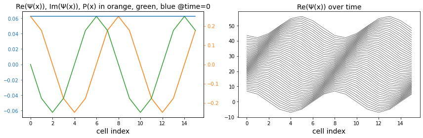
Figure 1: A plane wave of two periods moves rightwards in a cellular automaton of 16 cells over 40 iterations. The orange (green) curve shows the real (imaginary) part of $\Psi(x,t\!=\!0)$ and the blue curve $P(x,t\!=\!0)$. The stack of black curves shows the real part of $\Psi(x,t)$ for $0\leq t<40$.

The integrated probability $P$ remains very close to $1$. After as many as 100k cycles $\mid\!P\!-\!1\!\mid\;\approx 10^{-11}$, without any form of normalization. The plane wave moves rightwards and its shape is well preserved over time. The phase velocity, as measured from this simulation, is a little over 4 cells per 40 cycles, $\approx 0.1$.

Below the phase velocity is derived as a function of $\theta$ and $k$. Cell index $x$ refers to an even-numbered cell and $\Psi(x,t_{0})$ at time $t_{0}$ is a plane wave with $x_{0}\!=\!0$. (For odd-numbered cells the expression is slightly different.) The state of the automaton after a single iteration is described by $\Psi(x,t_{0}\!+\!1)$.

$$\begin{array}[]{lll}\Psi(x,t_{0})&=&e^{ikx}\\ \Psi(x,t_{0}\!+\!1)&=&e^{ikx}e^{2i\theta}\big{(}-\!\sin^{2}(\theta)e^{-2ik}+\frac{1}{2}i\sin(2\theta)e^{-ik}+\cos^{2}(\theta)+\frac{1}{2}i\sin(2\theta)e^{ik}\big{)}\\ &=&e^{ikx}e^{2i\theta}\big{(}\cos^{2}(\theta)-\sin^{2}(\theta)e^{-2ik}+i\sin(2\theta)\cos k\big{)}\\ &=&e^{ik(x-v_{p}(\Delta t=1))}~{},\\ \mathrm{where}~{}~{}v_{p}&=&\frac{1}{k}\Big{(}2\theta-\mathrm{arg}\big{(}\cos^{2}(\theta)-\sin^{2}(\theta)e^{-2ik}+i\sin(2\theta)\cos(k)\big{)}\Big{)}~{}.\end{array}$$ (3.3)

For sufficiently small values of $\theta$, phase velocity $v_{p}$ can be approximated by

$$v_{p}(\theta,k)\approx 2\theta\Big{(}\frac{1-\cos k}{k}\Big{)}~{}.$$ (3.4)

From the Taylor expansion of $\cos k$ it immediately follows that $\lim_{k\rightarrow 0}v_{p}(\theta,k)=0$. For the experiment of Figure 1 this results in $v_{p}(\frac{\pi}{24},\frac{\pi}{4})=0.098$, in nice agreement with the observed phase velocity. Figure 2 depicts the exact and approximate phase velocities. The “smallness of $\theta$” assumption in practice apparently means $\theta\!<\!\frac{\pi}{8}$.

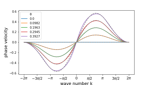
Figure 2: Phase velocity $v_{p}$ versus wave number k, $k\in[-2\pi,2\pi)$, for various $\theta$ in units of $\frac{a}{\tau}$ The colored curves are based on Identity 3.3 and the dashed grey curves are approximations based on 3.4.

3.2 A homogeneous CA with periodic boundaries: wavepackets

In the next experiment the same cellular automaton is initialized with a wavepacket of the form $W_{\mathit{p}acket}$, using a normalization constant $A$

$$W_{\mathit{p}acket}(x,x0,\sigma,k)=A\;e^{-\frac{1}{2}\big{(}\frac{x-x_{0}}{\sigma}\big{)}^{2}}e^{ik(x-x_{0})}~{}.$$ (3.5)

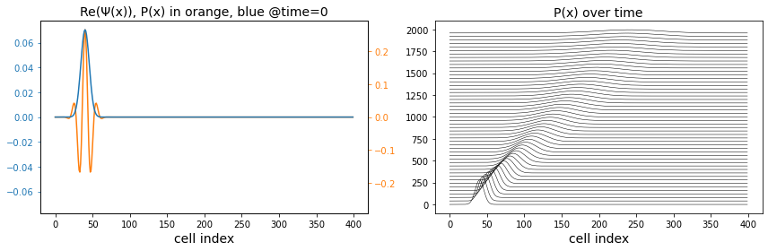
Figure 3: A short wavepacket moves rightwards in a periodic cellular automaton of 400 cells over 8000 iterations.

Figure 3 shows a wavepacket $W_{\mathit{p}acket}$, centered around position $x_{0}\!=\!40$ with $\sigma\!=\!8$ and $k\!=\!\frac{\pi}{8}$. Note that the spatial extent of the wavepacket appears to be less than three wavelengths. The automaton is evolved over 2000 cycles, and its probability density is plot at fixed intervals. The wavepacket moves rightwards rather slowly, fewer than 200 cells in 2000 cycles. Furthermore, it rapidly disperses over a wide range.

A wavepacket is composed of a finite set of component sinusoidal waves of different wave numbers, each propagating with its own wavenumber-dependent velocity. The wavepacket in Figure 3 has a center $k\!=\!\frac{\pi}{8}$. Component waves with a lower $k$ move slower and those with a higher $k$ faster. It is common to derive the phase velocity from the so-called dispersion relation $\omega(k)$. Conversely, from (3.4) it follows that

$$\omega(k)~{}=~{}kv_{p}~{}\approx~{}2\theta(1-\cos k)~{}.$$ (3.6)

In Figure 4 the same automaton is initialized with a different wavepacket, with $\sigma\!=\!8$ and $k\!=\!\frac{\pi}{2}$. Roughly ten wavelengths fit in the Gaussian envelope. This automaton is evolved over 8000 cycles and the wavepacket envelope is drawn every 200 cycles.

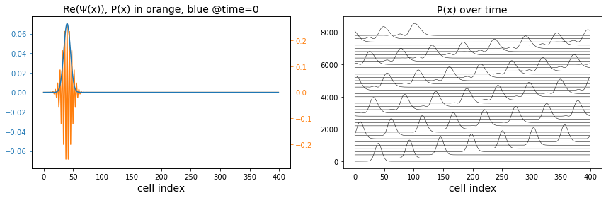
Figure 4: A long wavepacket moves rightwards in a periodic cellular automaton of 400 cells over 8000 iterations.

After a couple of thousand cycles the dispersion of the packet becomes visible as a minor pulse trailing the main pulse. Compared to the previous experiment, the dispersion is substantially less, because of the smaller bandwidth $\Delta k/k$ of the wavepacket. The component wave of the center frequency ($k\!=\!\frac{\pi}{2}$) moves fastest; all the other component waves move slower. (Recall that with $k\!=\!\frac{\pi}{2}$ the phase velocity of the center frequency of the wavepacket is zero.) It takes about 1600 cycles for a packet to traverse the width of the cellular automaton, and to reappear at the left hand side. The measured group velocity is $\approx$ 0.26 cells per cycle. The phase velocity $v_{p}$ and group velocity $v_{g}$ are related by

$$v_{p}=\frac{\omega}{k}\hskip 56.9055pt\mathrm{and}\hskip 56.9055ptv_{g}=\frac{d\omega}{dk}~{}.$$ (3.7)

Then from Identity 3.4 and for sufficiently small values of $\theta$

$$v_{g}~{}~{}=~{}~{}\frac{d(kv_{p})}{dk}~{}~{}\approx~{}~{}-2\theta\frac{d\cos k}{dk}~{}~{}=~{}~{}2\theta\sin k~{}.$$ (3.8)

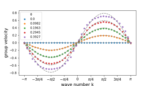
Figure 5: Group velocity $v_{g}$ versus wave number $k$, $k\in[-\pi,\pi)$, for various $\theta$ in units of $\frac{a}{\tau}$. The colored $\star$ markers denote measured group velocities from cellular automata evolutions. The dashed grey lines are based on the approximation of Identity 3.8.

Figure 5 shows the measured group velocity $v_{g}$ versus $(\theta,k)$. These measurements are based on the displacement of the peak of the Gaussian envelope of the wavepacket during a time interval of 200 cycles. The group velocity is periodic in $k$, approximately sinusoidal. It is well known that imposing periodic boundary conditions in space leads to discrete momenta. It is less wel known is that discretization of space leads to periodic momenta. The momentum interval $[-\pi,\pi)$, used to depict $v_{g}(k)$, is known as the Brillouin zone.

3.3 An infinite potential well: eigen states

The next cellular automaton models an infinite square well (see e.g. [1]). The experiment is also known as a particle in a box. The box has length $L$ and is centered around $x_{c}$. Inside the box, $x_{c}\!-\!\frac{L}{2}<x<x_{c}\!+\!\frac{L}{2}$, the potential equals 0, iutside the box it is infinite, and $\Psi_{n}(x,t)=0$. This infinite potential is modelled by applying two-by-two building block $\pi\mathbf{B}^{\prime}$ (Definition 2.22) at the well boundaries.

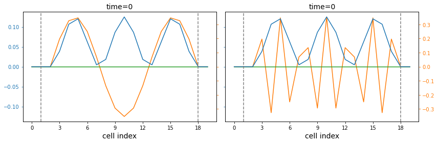
Figure 6: A cellular automaton with an infinite potential well with $L\!=\!16$ and $x_{c}\!=\!10$, initialized with $W_{\mathit{b}ox}(\ldots,3)$ (left) and with $W_{\mathit{b}ox}(.\ldots,L\!-\!3)$ (right).

The cellular automaton comprises 18 cells. With the applicable boundary conditions, the initial state is chosen to according to $W_{\mathit{b}ox}$, for integer $n\geq 0$

$$W_{\mathit{b}ox}(x,x_{c},L,n)=\sqrt{\frac{2}{L}}\sin\big{(}\frac{n\pi}{L}(x-x_{c}+L/2)\big{)}~{}.$$ (3.9)

Similar to $W_{\mathit{p}lane}$ (see Subsection 3.1), $W_{\mathit{b}ox}$ is subject to spatial aliasing: $W_{\mathit{b}ox}(x,x_{c},L,n)=W_{\mathit{b}ox}(x,x_{c},L,2L\!+\!n)$. Interestingly, there is another, somewhat more subtle, symmetry. Let $\Psi_{n}(t\!=\!0)=W_{\mathit{b}ox}(x,x_{c},L,n)$ and $\Psi_{L-n}(t\!=\!0)=W_{\mathit{b}ox}(x,x_{c},L,L\!-\!n)$. For $t\geq 0$, the corresponding $P(x,t)$ evolve in the same way, that is, $\mid\!{\Psi_{n}(x,t)}\!\mid^{2}\;=\;\mid\!{\Psi_{L-n}(x,t)}\!\mid^{2}$. This symmetry is illustrated in Figure 6 for $L\!=\!16$ and $n\!=\!3$.

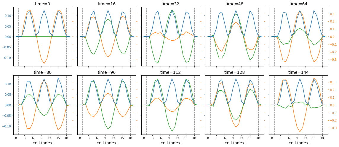
Figure 7: The evolution of the infinite-square-well automaton with $L\!=\!16$. The colors orange, green, and blue denote $\mathrm{Re}(\Psi_{3}(x,t))$, $\mathrm{Im}(\Psi_{3}(x,t))$, and $P(\Psi_{3}(x,t))$ respectively.

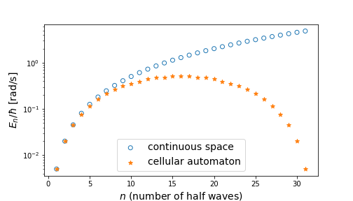
Figure 8: The energy levels $E_{n}/\hbar$ (in units of $\textrm{rad}/s$) versus $n$ for an infinite square well.

Figure 7 shows the evolution of the automaton for $n\!=\!3$. This evolution is periodic over time with a period of about 141 cycles. The analytic solution for $\Psi_{n}(x,t)$ for continuous space is well known, see e.g. [1],

$$\Psi_{n}(x,t)=\sqrt{\frac{2}{L}}\sin\Big{(}k_{n}\big{(}x-x_{c}+\frac{L}{2}\big{)}\Big{)}e^{-i\omega_{n}t}~{},$$ (3.10)

where $k_{n}=\frac{n\pi}{L}$. The corresponding energy levels are

$$\frac{E_{n}}{\hbar}~{}=~{}\omega_{n}~{}=~{}\frac{n^{2}\pi^{2}\hbar}{2mL^{2}}~{}=~{}n^{2}\pi^{2}\Big{(}\frac{a}{L}\Big{)}^{2}\;\frac{\theta}{\tau}~{}.$$ (3.11)

Figure 8 shows $E_{n}/\hbar$ versus $n$ for a cellular automaton with $L\!=\!16a$, $\theta\!=\!\pi/24$, and $\tau\!=\!1$. The orange stars are derived from the measured oscillation periods during the evolution of the cellular automaton initialized with $W_{\mathit{b}ox}(\ldots,n)$. The blue circles represent Identity 3.11. The number of energy levels $E_{n}$ for the automaton is finite, namely $L\!-\!1$. Moreover, energy $E_{n}$ is symmetric in $n\!=\!L$ and periodic with period $2L$, as an immediate consequence of the earlier noted spatial aliasing resulting from the sampling of $W_{\mathit{b}ox}$.

3.4 An infinite potential well: wavepackets

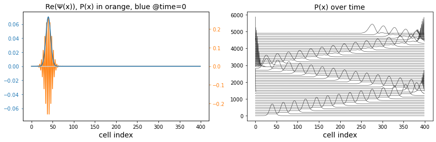
Figure 9: A wavepacket in a cellular automaton of 400 cells with reflective boundaries.

The cellular automaton of Figure 9 has hard boundaries, with $\pi\mathbf{B}^{\prime}$ (Definition 2.22) for the right-most cell. The initial wavepacket has the same parameters as before: $\sigma\!=\!8$ and $k\!=\!\frac{\pi}{2}$. During an evolution of 5000 cycles, the wavepacket reflects three times at the boundary of the cellular automaton. With each bounce the wavepacket interferes with itself and subsequently nicely recovers. Some dispersion can be observed towards the end of the simulation.

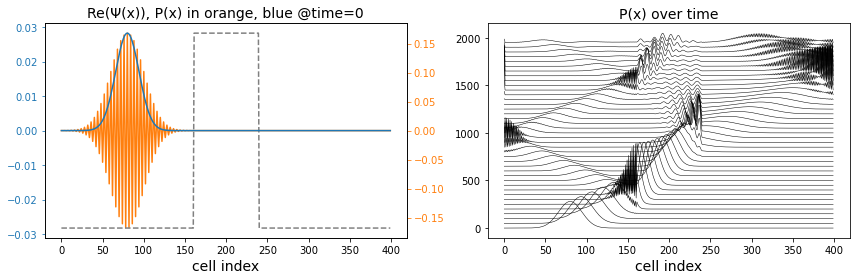
Figure 10: A wavepacket in a cellular automaton of 400 cells with hard boundaries, and a region in the middle with an increased potential energy of $V=0.12\delta$.

The cellular automaton of Figure 10 has hard boundaries similar to the previous one. Furthermore it has a narrow region in the middle with an increased potential $V(x)=0.12\delta$, as indicated by the light gray line. This automaton mimics the refraction of a particle through a glass slab with a higher refractive index. The automaton runs for 2000 cycles. The wavepacket hits the high-$V(x)$ region around $t\!=\!250$. A smaller part is reflected, and the main part of the wavepacket proceeds into this region at a lower group velocity and with a reduced width. Around $t\!=\!900$ the packet hits the backside of the high-$V(x)$ region, where, again, a smaller part is reflected and the main part continues.

3.5 A harmonic oscillator

The harmonic oscillator is based on a potential energy function that is parabolic in $x$, $V(x)=\frac{1}{2}m\omega^{2}x^{2}$. Its eigen states are well known and described here as $W_{\mathit{h}armonic}(x,n)$

$$W_{\mathit{h}armonic}(x,n)=A\;\frac{1}{\sqrt{2^{n}n!}}H_{n}(x)e^{-x^{2}/2}~{},$$ (3.12)

where $H_{n}(x)$ is the Hermite polynomial of degree $n$, and $A$ a normalization constant.

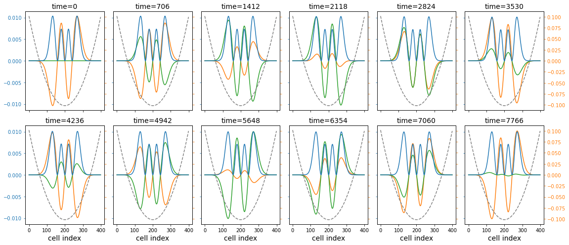
Figure 11: The evolution of a harmonic-oscillator CA initialized with $W_{\mathit{h}armonic}(x,3)$. The dashed parabola represent $V(x)$. The measured oscillation period is 7764 cycles.

Figure 11 shows the evolution of a cellular automaton with $V(x)/\delta\!=5.10^{-8}(x\!-\!200)^{2}$, initialized with $W_{\mathit{h}armonic}(x,3)$, where the state is captured every 706 cycles. The probability distribution $P(x,t)$ is constant over the entire episode of 7766 cycles and a single oscillation period lasts about 7764 cycles. This period corresponds to $\omega_{n}=2\pi/7764\approx 0.0008$ radians per second.

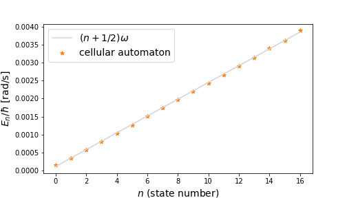
Figure 12: The energy levels $E_{n}/\hbar$ of the harmonic oscillator. The orange stars show the measured frequencies $\omega_{n}$ of $\Psi_{n}(x,t)$ and the gray curve shows $(n+\frac{1}{2})\omega$.

Figure 12 shows the energy levels $E_{n}/\hbar$ for $0\leq n<17$. Each datapoint is obtained by initializing the cellular automaton with the corresponding eigen state, and evolving the automaton until it revisits that eigenstate. The energy level $E_{n}/\hbar$ then equals the reciprocal value of that time interval. The measured results agree with the $(n+\frac{1}{2})\hbar\omega$ energy levels expected from theory.

4 Experiments with 2D cellular automata

This section presents a 2D refraction experiment and a double-slit experiment applying the ideas on 2D cellular automata as introduced in Subsection 2.5.

4.1 Refraction

Figure 13 shows a refraction experiment which is a 2D generalization of the 1D refraction automaton of 10. The (shaded) horizontal region in the middle has a higher potential. The 2D wavepacket partially bounces off that region, around $t\!=\!400$, and partially propagates through that region at a reduced velocity ($t\!=\!600$). Around $t\!=\!1200$ the reduced packet further splits into two parts, one escaping from the high-$V$ region, and one remaining inside.

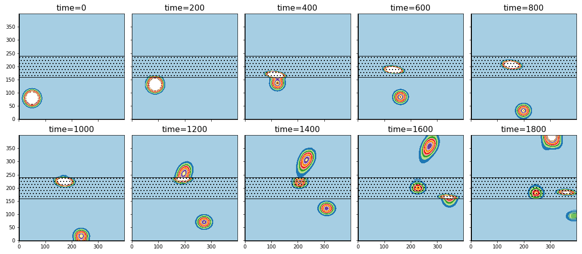
Figure 13: A refraction experiment of a 2D wavepacket interacting with a high-$V$ region (shaded). The colors show different values of $\mid\!{\Psi}\!\mid^{2}$, from blue (low) to white (high).

4.2 Double-slit experiment

The double-slit experiment demonstrates quantum interference of a single massive particle, both constructive and destructive. Feynman describes this form of interference as “a phenomenon which is impossible, absolutely impossible, to explain in any classical way, and which has in it the heart of quantum mechanics” [12].

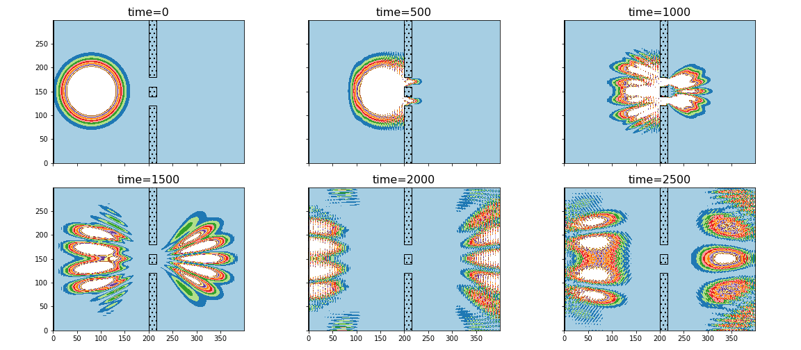
Figure 14: Double-slit diffraction, where colors show different values of $\mid\!{\Psi}\!\mid^{2}$, with white for larger values and blue for smaller values.

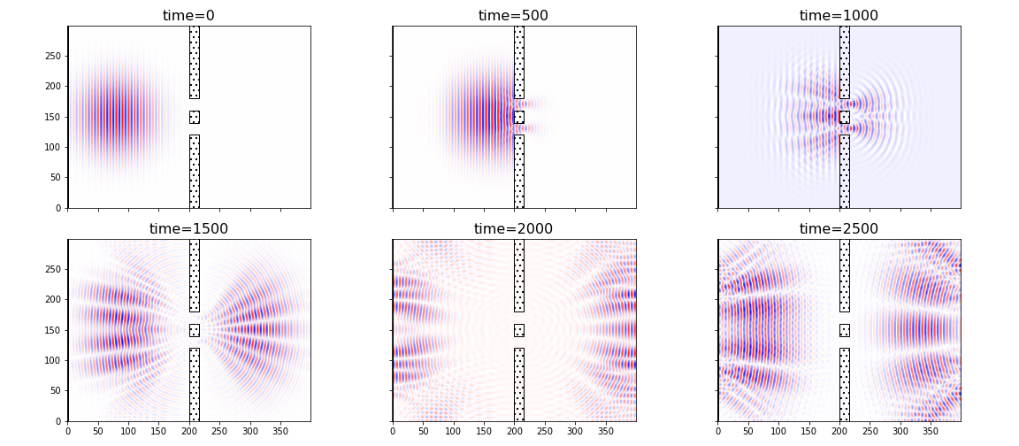
Figure 15: The same double-slit diffraction experiment, as in Figure 14, where colors show different values of $\textrm{Re}(\Psi)$, red for positive values and blue for negative values.

The double-slit cellular automaton of Figure 14 is centered around a vertical screen (shaded) with a thickness of 16 cells. The slits are 20 cells wide, and separated (heart-to-heart) by 40 cells. The rotation angle of the automaton $\theta\!=\!\frac{\pi}{24}$. The initial two-dimensional wave packet has an uncertainty in its intitial position of $\sigma\!=\!40$, and a wavevector $k\!=\!(\frac{\pi}{5},0)$, corresponding to a wavelength of $\lambda\!=\!10$ cells. The result of the evolution of the cellular automaton is depicted for five intervals of 500 cycles. Note that the wavepacket diffracts at both sides of the screen, causing interference fringes at either side. These fringes are subsequently reflected by the boundaries of the automaton.

Figure 14 shows the computed probability densities of a single particle, unlike in practical experiments where the interference emerges only after many independent particles. The result of the evolution of the cellular automaton look similar to those obtained by simulation of the Schrödinger equation using the Crank-Nicolson numerical method [5]. Figure 15 shows the evolution of the real part of $\Psi$.

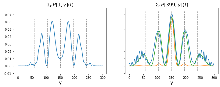
Figure 16: The double-slit quantum interference (in blue) observed at $x\!=\!1$ (left) and at $x\!=\!399$ (right). The orange and green curves are explained in the text.

Figure 16 shows the interference patterns at the left and right hand sides of the automaton. The distance $D$ between the interference peaks on the right hand side $D$ is given by the well-known expression $D\!=\!\lambda l/d$, and is marked by the gray dashed lines. The intensity values at these peaks also depend on the slit widths $b$. If the width of the slits $b\!\gg\!\lambda$, the intensity $I(\phi)$ of the diffracted light is given by [13]:

$$I(\phi)\propto\cos^{2}\Big{(}\frac{\pi d\sin\phi}{\lambda}\Big{)}\;\mathrm{sinc}\Big{(}\frac{\pi b\sin\phi}{\lambda}\Big{)}~{},$$ (4.1)

where $\phi$ is the angle with respect to the horizontal from the midpoint between the slits towards the right plane. The $\cos^{2}()$ factor describes the interference pattern and the $\mathrm{sinc}()$ factor acts as an envelope. The orange curve in the right-hand-side panel shows $I(\phi)$ for the actual geometry. The green curve for a modified geometry, with the slit width reduced from $b\!=\!20$ to $b\!=\!4$. Apparently, the slit width of $b\!=\!20$ is too close to $\lambda\!=\!10$ for (4.1) to offer an accurate approximation.

5 Conclusion

The discrete Schrödinger equation for a single particle leads to a band matrix for the Hamiltonian $\mathbf{H}$. However, the corresponding evolution matrix $\mathbf{U}$ is dense, and therefore is not suitable as a cellular automaton. Matrix $\mathbf{H}$ can be written as the sum of two 2$\times$2 block-diagonal matrices (Definition 2.11), with corresponding evolution matrices $\mathbf{U}_{0}$ and $\mathbf{U}_{1}$. These matrices, together with their product $\mathbf{U}_{1}\mathbf{U}_{0}$, are unitary as well as band-structured. The Schrödinger cellular automata presented in this paper are based on this split evolution. Unitarity is demonstrated by the strict preservation of the integrated probability $P\!=\!1$ over many tens of thousands of evolution cycles.

This split evolution does not offer an exact solution of the Schrödinger equation. For low momentum $k$ (Fig. 5) and low energy levels $E_{n}$ (Fig. 8) the agreement with known analytical solutions is good. However, the group velocity appears to be periodic in $k$ (Fig. 5) and the energy of an infinite square well is periodic in the number of half waves $n$ (Fig. 8). These periodicity properties are not particular to the cellular automata, but follow from the discrete spatial sampling of the wave functions. Discretization of space unavoidably connects quantum physics to the realm of Nyquist rates and spatial aliasing.

What to make of these periodicities? It is sometimes conjectured that if physical time and space are discrete then this is so at the Planck scale, see e.g. [2, 3]. At the Planck scale, the cell size is approximately the Planck length ($a\approx l_{P}$), the time step approximately the Planck time ($\tau\approx t_{P}$), and the speed of light $c=l_{P}/t_{P}\approx a/\tau$. A particle with a wavelength $\lambda=2a=2l_{P}$ would have an energy $h\nu=\frac{1}{2}hc/l_{P}\approx 4\cdot 10^{28}eV$. This value is many orders of magnitude beyond the 13.6 TeV of the LHC and the $\approx 3\cdot 10^{20}eV$ of the most energetic cosmic-ray particles observed. This discrepancy suggests that for “realistic” physics the wavelengths exceed hundreds or perhaps thousands of cell sizes, consistent with the low-energy approximation of discrete space and time.

Fig. 5 suggests that the group velocity peaks at close $a/\tau\!=\!c$. However, it does so for $k=\pi(\frac{1}{2}+2n)$, which clearly is not relativistic. Unsurprisingly, the Schrödinger equation cannot teach us a lot about relativistic behavior. Cellular automata based on the Klein-Gordon equation or on the Dirac equation [3] may hold more promise in this respect.

Multi-dimensional cellular automata can be constructed from lower-dimensional cellular automata (Subsection 2.5), with a two-dimensional version of the double-slit experiment (Subsection 4.2) as an example. The underlying evolution matrices are intrinsically sparse and unitary, enabling a dramatic reduction in computational effort compared to conventional numeric simulations. In a three-dimensional form, scaled to many billions of cells, and powered by – possibly tailored – High-Performance Compute hardware, Schrödinger Unitary Cellular Automata may offer a new tool for quantum-physical exploration. They provide 1) full control over boundaries, $V(x)$, and the initial state at cell granularity, 2) a possible reduction to two dimensions, and 3) observability at high spatial and temporal resolution.

References

- [1] D. J. Griffiths and D. F. Schroeter, Introduction to quantum mechanics. Cambridge ; New York, NY: Cambridge University Press, third edition ed., 2018.
- [2] Gerard ’t Hooft, The Cellular Automaton Interpretation of Quantum Mechanics. Springer, 2015.
- [3] A. Bisio, G. M. D’Ariano, and A. Tosini, “Quantum field as a quantum cellular automaton: The dirac free evolution in one dimension,” Annals of Physics, vol. 354, pp. 244–264, 2015.
- [4] J. Crank and P. Nicolson, “A practical method for numerical evaluation of solutions of partial differential equations of the heat-conduction type,” Advances in Computational Mathematics, vol. 6, pp. 207–226, 1947.
- [5] Mena, A, “Solving the 2D Schrödinger equation using the Crank-Nicolson method.” https://artmenlope.github.io/solving-the-2d-schrodinger-equation-using-the-crank-nicolson-method/, 2023. [Online; accessed 23-Mar-2024].
- [6] Toffoli, Tommaso and Margolus, Norman, Cellular Automata Machines: A New Environment for Modeling. MIT Press, 04 1987.
- [7] I. Bialynicki-Birula, “Weyl, dirac, and maxwell equations on a lattice as unitary cellular automata,” Physical review D: Particles and fields, vol. 49, pp. 6920–6927, 07 1994.
- [8] G. Grössing and A. Zeilinger, “Quantum cellular automata,” Complex Syst., vol. 2, p. 197–208, apr 1988.
- [9] P. Arrighi, “An overview of quantum cellular automata,” Natural Computing, vol. 18, no. 4, pp. 885–899, 2019.
- [10] T. Farrelly, “A review of Quantum Cellular Automata,” Quantum, vol. 4, p. 368, Nov. 2020.
- [11] A. T. Sornborger and E. D. Stewart, “Higher-order methods for simulations on quantum computers,” Phys. Rev. A, vol. 60, pp. 1956–1965, Sep 1999.
- [12] R. P. Feynman, R. B. Leighton, and M. Sands, The Feynman lectures on physics: The Definitive Edition (Vol. 3). Pearson, 2009.
- [13] F. Jenkins and H. White, Fundamentals of Optics. International student edition, McGraw-Hill, 1976.