Family of Exact and Inexact Quantum Speed Limits for Completely Positive and Trace-Preserving Dynamics

Abstract

Traditional quantum speed limits formulated in density matrix space perform poorly for dynamics beyond unitary, as they are generally unattainable and fail to characterize the fastest possible dynamics. To address this, we derive two distinct quantum speed limits in Liouville space for Completely Positive and Trace-Preserving (CPTP) dynamics that outperform previous bounds. The first bound saturates for time-optimal CPTP dynamics, while the second bound is exact for all states and all CPTP dynamics. Our bounds have a clear physical and geometric interpretation arising from the uncertainty of superoperators and the geometry of quantum evolution in Liouville space. They can be regarded as the generalization of the Mandelstam-Tamm bound, providing uncertainty relations between time, energy, and dissipation for open quantum dynamics. Additionally, our bounds are significantly simpler to estimate and experimentally more feasible as they require to compute or measure the overlap of density matrices and the variance of the Liouvillian. We have also obtained the form of the Liouvillian, which generates the time-optimal (fastest) CPTP dynamics for given initial and final states. We give two important applications of our bounds. First, we show that the speed of evolution in Liouville space bounds the growth of the spectral form factor and Krylov complexity of states, which are crucial for studying information scrambling and quantum chaos. Second, using our bounds, we explain the Mpemba effect in non-equilibrium open quantum dynamics.

In non-equilibrium quantum dynamics, a fundamental problem is to understand the pace at which quantum systems dissipate, decohere, or approach a stationary state when they are subjected to external environments and fields. Currently, this problem has become one of the focal points of research, considering the importance of understanding the pace of many interesting physical phenomena such as the so-called quantum version of the Mpemba effect [1, 2, 3], relaxation processes in open quantum systems [4, 5], the growth of spread and Krylov complexity [6, 7, 8, 9, 10], information scrambling [11], etc. This issue also holds significant practical relevance in the rapidly developing field of quantum information technologies, as the pace of the dynamics impacts the performance of quantum devices such as quantum thermal and energy storage devices. Hence, it is crucial to understand the general properties of non-equilibrium quantum dynamics, which sets the pace at which dynamics occur.

In physical processes, the rate at which the state of a quantum system changes in the state space is referred to as the speed of evolution (pace of dynamics). The rate of change of the distinguishability between the initial and time-evolved states is constrained by the evolution speed, leading to a lower bound on the evolution time. This bound represents inherent dynamical limitations in quantum physics and is referred as the quantum speed limit (QSL). The first such bound was the Mandelstam-Tamm (MT) bound [12], which was derived for unitary dynamics generated by a time-independent Hamiltonian using the Robertson uncertainty relation, and later using the geometry of quantum evolution [13]. The MT bound states that the evolution time is lower bounded by the ratio of the Hilbert space angle between the initial and final states to the speed of evolution in the state space, i.e., the variance of the Hamiltonian in the initial state. This bound provides an unambiguous meaning to the time-energy uncertainty relation [14, 15] and saturates for the fastest unitary dynamics [16, 17]. Recently, the exact form of the MT bound has been obtained for arbitrary unitary dynamics, which can determine the exact time required to implement any unitary operation [18]. The MT bound has also been extended to the unitary dynamics of operators [19, 20, 21, 22, 23], superoperators [24], and entanglement [25], as well as various classical dynamics [26, 27], and non-Hermitian quantum dynamics [28, 29, 30]. Recently, several experiments have verified the MT bound [31, 32], which has numerous applications in rapidly growing quantum technologies [33, 34, 35, 36].

In the last decade, various generalized quantum speed limits (QSLs) have been formulated for more general types of quantum dynamics using mathematical inequalities [37, 38, 39, 40, 41, 42, 43, 44] and the geometry of density matrix space [45, 46, 47, 48]. Most of these QSLs are challenging to compute for a wide class of quantum dynamics, especially as the system’s dimension or the complexity of the dynamics increases. This difficulty arises because they generally require estimating norms of non-Hermitian operators, the quantum Fisher information, and the square roots of density matrices. In general, these QSLs are not attainable for a wide class of dynamics due to (i) the presence of classical uncertainty within the states, and (ii) some parts of the generator of the dynamics may not contribute to the change of the distinguishability. Along with this, they fail to characterize the generator of dynamics which induces the time-optimal (fastest) process. Moreover, these QSLs do not resemble the MT bound, as they do not depend on the variance of the generator of the dynamics. Consequently, they may not fully capture the dynamical properties needed to control the pace of dynamics, as the MT bound does for unitary dynamics [49, 50, 51, 52]. Furthermore, these speed limits provide a lower bound on the evolution time rather than an exact relation. Thus, the true generalization of the MT bound, which offers a time-energy-dissipation uncertainty relation in its exact form for Completely Positive Trace-Preserving (CPTP) dynamics (which describes the wide class of physical processes), remains an important question. Recent studies of open quantum systems utilize Liouville space descriptions. Therefore, it is also crucial to formulate speed limits for states in Liouville space rather than in density operator space.

In this article, we derive exact and inexact quantum speed limits for CPTP dynamics for finite-dimensional quantum systems in Liouville space. First, we derive an inexact quantum speed limit using the uncertainty relation for non-Hermitian superoperators. This provides a lower bound on the evolution time, defined as the ratio of the Liouville space angle between the initial and final states to the time-averaged variance of the Liouvillian (i.e., generator of the CPTP dynamics). This bound establishes a time-energy-dissipation uncertainty relation and can be regarded as the generalized form of the original Mandelstam-Tamm (MT) bound. We show that this bound is saturated for time-optimal CPTP dynamics, which drives the system along the geodesic in Liouville space. Since this bound is an inequality, we then derive the exact generalization of the MT bound for CPTP dynamics for finite-dimensional quantum systems using the exact uncertainty relation for superoperators. We show that the evolution time can be exactly expressed as the ratio of the analogous Wootters distance in Liouville space, which connects the initial and final states, to the variance of the non-classical part of the Liouvillian since the classical part of the Liouvillian commutes with the initial state and does not contribute to the change in distinguishability. We have also provided geometrical interpretation to both bounds using the geometry of quantum evolution in Liouville space. Additionally, we show two important applications of our results. First, we show that our speed limit sets bounds on the spectral form factor and Krylov complexity of states, which are important quantities for studying information scrambling and quantum chaos. Second, our speed limits reveal why states far from equilibrium can relax more quickly than those near equilibrium. This insight naturally explains the Mpemba effect in open quantum dynamics.

We begin by presenting preliminary results that are essential for arriving at our main findings.

Liouville Space: For every linear operator $A=\sum_{ij}\alpha_{ij}\outerproduct{i}{j}$ acting on a $d$-dimensional Hilbert space $\mathsf{H}_{d}$, there exists a vector $|A)=\sum_{ij}\alpha_{ij}\ket{j}\otimes\ket{i}$. These vectorized linear operators form a Hilbert space $\mathsf{H}_{d}\otimes\mathsf{H}_{d}$ also known as Liouville space, with the inner product $(A|B):=\operatorname{tr}{(A^{\dagger}B)}$ [53]. The operators acting on Liouville space are called superoperators. In Liouville space, arbitrary CPTP dynamics is described by the following master equation (see Appendix A):

$$\frac{d}{dt}|{\tilde{\rho}_{t}})=\left(\mathcal{L}_{t}-\frac{1}{2}\left\{(\tilde{\rho}_{t}|\mathcal{L}_{t}|\tilde{\rho}_{t})+(\tilde{\rho}_{t}|\mathcal{L}_{t}^{\dagger}|\tilde{\rho}_{t})\right\}\right)|{\tilde{\rho}_{t}}),$$ (1)

where $\mathcal{L}_{t}$ is the generator of the dynamics and is known as the Liouvillian superoperator, and $\mathcal{L}^{\dagger}_{t}$ is its adjoint. The term $|\tilde{\rho}_{t}):=\frac{|\rho_{t})}{\norm{|\rho_{t})}}$ represents the normalized state vector corresponding to the time-evolved density matrix $\rho_{t}$, with $\norm{|\rho_{t})}=\sqrt{\operatorname{tr}{(\rho_{t}^{2})}}$ representing the Hilbert-Schmidt norm of $\rho_{t}$. For the rest of the article, we drop the subscript ’$t$’ from $\mathcal{L}_{t}$ and assume that the Liouvillian is time-dependent unless stated otherwise. We assume $\hbar=1$ throughout this work.

Exact and Inexact Uncertainty Relations for Superoperators: Here, we present two uncertainty relations for superoperators: one as an inequality (inexact) and the other as an equality (exact).

Proposition 1.

For any two non-Hermitian superoperators $\mathcal{A}$ and $\mathcal{B}$, there exists an uncertainty relation given by

$$(\Delta\mathcal{A})^{2}(\Delta\mathcal{B})^{2}\geq\left|\operatorname{tr}(\mathcal{A}^{\dagger}\mathcal{B}\mathcal{P})-\operatorname{tr}(\mathcal{A}^{\dagger}\mathcal{P})\operatorname{tr}(\mathcal{B}\mathcal{P})\right|^{2},$$ (2)

where $\mathcal{P}:=|\tilde{\rho})(\tilde{\rho}|$ represents the projection superoperator corresponding to the state vector $|\tilde{\rho})$, and $\operatorname{tr}(\mathcal{O}\mathcal{P})$ and $(\Delta\mathcal{O})^{2}=\operatorname{tr}(\mathcal{O}^{\dagger}\mathcal{O}\mathcal{P})-\operatorname{tr}(\mathcal{O}^{\dagger}\mathcal{P})\operatorname{tr}(\mathcal{O}\mathcal{P})$ are the average and the variance of the superoperator $\mathcal{O}$ in the state vector $|\tilde{\rho})$.

Proposition 2.

For any Hermitian superoperator $\mathcal{A}$ and a non-Hermitian superoperator $\mathcal{B}$, there exists an exact uncertainty relation for all state vectors $|\tilde{\rho})$ given by

$$\delta_{\mathcal{B}}\mathcal{A}\Delta\mathcal{B}_{nc}=\frac{1}{2},$$ (3)

where $\mathcal{B}_{nc}=\mathcal{B}-\mathcal{B}_{cl}$ is the non-classical (non-diagonal) part of $\mathcal{B}$ in the basis of $\mathcal{A}$, i.e., $\{|a_{i})\}$, and $\delta_{\mathcal{B}}\mathcal{A}$ is the uncertainty of the superoperator $\mathcal{A}$ in the state vector $|\tilde{\rho})$, defined as

$$(\delta_{\mathcal{B}}\mathcal{A})^{-2}:=\sum_{i}\frac{(a_{i}|\mathcal{G}|a_{i})^{2}}{(a_{i}|\mathcal{P}|a_{i})},\quad\mathcal{B}_{cl}:=\sum_{i}|a_{i})(a_{i}|\frac{(a|\mathcal{C}|a_{i})}{(a_{i}|\mathcal{P}|a_{i})},$$ (4)

where $\mathcal{G}:=(\mathcal{B}\mathcal{P}+\mathcal{P}\mathcal{B}^{\dagger}-\mathcal{P}\operatorname{tr}[\mathcal{P}(\mathcal{B}+\mathcal{B}^{\dagger})])$, $\mathcal{C}:=\frac{i}{2}(\mathcal{B}\mathcal{P}-\mathcal{P}\mathcal{B}^{\dagger})$ and $\mathcal{B}_{cl}$ is the classical part of $\mathcal{B}$ that commutes with $\mathcal{A}$.

The proof and details of the above uncertainty relations are provided in the Appendix A.

Now, we will discuss the main results of this article, beginning with the derivation of the inexact quantum speed limit for arbitrary CPTP dynamics for finite-dimensional quantum systems.

Theorem 1.

For a $d$-dimensional quantum system, the lower bound on the evolution time required to evolve a given state $\rho_{0}$ to a final state $\rho_{T}$ under a CPTP dynamics generated by the Liouvillian $\mathcal{L}$ is given by

$$T\geq\frac{\Theta(\rho_{0},\rho_{T})}{\langle\!\langle\Delta\mathcal{L}\rangle\!\rangle_{T}},$$ (5)

where $\Theta(\rho_{0},\rho_{T}):=\arccos{(\tilde{\rho}_{0}|\tilde{\rho}_{T})}$ is the Liouville space angle between the state vectors $|\tilde{\rho}_{0})$ and $|\tilde{\rho}_{T})$, corresponding to the initial and final states $\rho_{0}$ and $\rho_{T}$, respectively, $\Delta\mathcal{L}$ is the variance of the Liouvillian in the time-evolved state vector $|\tilde{\rho}_{t})$, and $\langle\!\langle X_{t}\rangle\!\rangle_{T}:=\frac{1}{T}\int_{0}^{T}\,dtX_{t}$ is the time average of $X_{t}$.

Proof.

Consider a $d$-dimensional quantum system with the initial state represented by the density matrix $\rho_{0}$ evolving under a CPTP dynamical map generated by an arbitrary Liouvillian $\mathcal{L}$. The rate of change of the distinguishability between the initial state vector $|\tilde{\rho}_{0})$ and the time-evolved state vector $|\tilde{\rho}_{t})$ using Eq. (1) can be written as

$$\frac{d}{dt}(\tilde{\rho}_{0}|\tilde{\rho}_{t})^{2} =\operatorname{tr}\left(\mathcal{L}\mathcal{P}_{t}\mathcal{P}_{0}\right)-\operatorname{tr}\left(\mathcal{P}_{t}\mathcal{P}_{0}\right)\operatorname{tr}((\mathcal{L}+\mathcal{L}^{\dagger})\mathcal{P}_{t})$$

$$\quad+\operatorname{tr}(\mathcal{P}_{t}\mathcal{L}^{\dagger}\mathcal{P}_{0}),$$ (6)

where $\mathcal{P}_{t}=|\tilde{\rho}_{t})(\tilde{\rho}_{t}|$ and $\mathcal{P}_{0}=|\tilde{\rho}_{0})(\tilde{\rho}_{0}|$. Taking the absolute value of both sides and using the uncertainty relation for non-Hermitian superoperators (2), we obtain the upper bound on the rate of change of distinguishability as

$$\left|\frac{d}{dt}(\tilde{\rho}_{0}|\tilde{\rho}_{t})^{2}\right|\leq 2\Delta\mathcal{L}\Delta\mathcal{P}_{0}\leq 2\Delta\mathcal{L},$$ (7)

where $(\Delta\mathcal{O})^{2}$ is the variance of the superoperator $\mathcal{O}$ in $|\tilde{\rho}_{t})$. The second inequality follows from the fact that $\Delta\mathcal{P}_{0}\leq 1$, indicating that the rate of change of the distinguishability of states (initial and time-evolved) is constrained by the speed of evolution in Liouville space. Integrating the first inequality on both sides and using the inequality $\left|\int f(t)\,dt\right|\leq\int|f(t)|\,dt$ before performing the integral, we obtain the bound 5. For the detailed proof of the theorem, refer to the Appendix B. ∎

The above theorem can be alternatively proved using the geometry of quantum evolution in Liouville space. In Liouville space, the infinitesimal distance $dS$ along the evolution path traced out by the state vector $|\tilde{\rho}_{t})$ can be expressed as

$$dS^{2}=\Delta\mathcal{L}^{2}dt^{2}.$$ (8)

From the above equation, we can obtain the speed of evolution (transportation) $dS/dt=\Delta\mathcal{L}$ of the quantum system under CPTP dynamics in the Liouville space, suggesting that the uncertainty of the Liouvillian in the time-evolved state drives the system forward in time. Integrating $\frac{dS}{dt}=\Delta\mathcal{L}$ on both sides and using the fact that the total path length $S$ traveled by the state in the Liouville space is lower bounded by the geodesic distance $\Theta(\rho_{0},\rho_{\text{T}})$ between the initial and final states of the system, i.e., $S\geq\Theta(\rho_{0},\rho_{\text{T}})$, we can obtain bound 5. Moreover, bound 5 can also be expressed in terms of the Kraus operators of the CPTP dynamical map instead of the Liouvillian, as well as it can be generalized beyond CPTP dynamics (see Appendix C).

For a dissipative process, the speed of evolution of a quantum system is time-dependent, even for a time-independent Liouvillian, because the Liouvillian is in general, a non-Hermitian superoperator. As a result, under such process, the norm is not preserved, i.e., $(\rho_{0}|e^{\mathcal{L}^{\dagger}t}e^{\mathcal{L}t}|\rho_{0})\neq(\rho_{0}|\rho_{0})$. Consequently, under such dynamics, quantum systems accelerate over time because the time derivative of the speed of evolution is non-zero. For a unitary process generated by a time-independent Liouvillian (an anti-Hermitian superoperator), the evolution speed is time-independent. Therefore, we do not need to solve the dynamics to estimate the lower bound for a unitary process. In general, for an arbitrary process, we can use the inequality $\Delta\mathcal{L}\leq\|\mathcal{L}\|_{\text{op}}$ (where $\norm{\mathcal{O}}_{\mathrm{o}p}$ is the largest singular value of the superoperator $\mathcal{O}$) to obtain a bound that does not require solving the dynamics.

The Liouvillian (obtained by vectorizing Lindblad master equation) can be decomposed into two parts as $\mathcal{L}=-i\mathcal{L}_{H}+\mathcal{L}_{D}$, where $\mathcal{L}_{H}:=\left(\mathbb{I}\otimes H_{t}-H_{t}^{T}\otimes\mathbb{I}\right)$ is associated with the Hamiltonian $H_{t}$, and $\mathcal{L}_{D}:=\sum_{k}\gamma_{k}\left(L^{k*}_{t}\otimes L^{k}_{t}-\frac{1}{2}\left(\mathbb{I}\otimes L^{k\dagger}_{t}L^{k}_{t}+(L^{k\dagger}_{t}L^{k}_{t})^{T}\otimes\mathbb{I}\right)\right)$ is associated with the dissipative part of the Lindblad master equation, where $\{\gamma_{k}\}$ are the decay rates and $\{L^{k}_{t}\}$ are the Lindblad operators. Using this decomposition, the square of the speed of evolution can be written as (see Appendix B)

$$\Delta\mathcal{L}^{2}={\Delta\mathcal{L}_{H}^{2}+\Delta\mathcal{L}_{D}^{2}+i\operatorname{tr}\left([\![\mathcal{L}_{H},\mathcal{L}_{D}]\!]\mathcal{P}_{t}\right)},$$ (9)

where $\Delta\mathcal{L}_{H}$ is the speed of the unitary part of the dynamics, $\Delta\mathcal{L}_{D}$ is the speed of the dissipative part of the dynamics, and $[\![\mathcal{L}_{H},\mathcal{L}_{D}]\!]:=(\mathcal{L}_{H}\mathcal{L}_{D}-\mathcal{L}^{\dagger}_{D}\mathcal{L}_{H})$ represents the non-commutativity of the unitary and the dissipative parts of the generator in the state $|\tilde{\rho}_{t})$. The last term in the above equation captures the nontrivial correlation between the unitary and dissipative speeds and is upper bounded by $2\Delta\mathcal{L}_{H}\Delta\mathcal{L}_{D}$. Since $\Delta\mathcal{L}_{H}$ is related to the uncertainty in energy and $\Delta\mathcal{L}_{D}$ is related to dissipation, the bound 5 can be regarded as time-energy-dissipation uncertainty relation. Therefore, the bound can be seen as the generalization of the original Mandelstam-Tamm bound, which was given for unitary dynamics [12, 13]. In the absence of the unitary part $\mathcal{L}_{H}$, it becomes the time-dissipation uncertainty relation. Alternatively, the Liouvillian can be decomposed into an anti-Hermitian and a Hermitian part as $\mathcal{L}=-i\mathcal{L}_{+}+\mathcal{L}_{-}$, where $\mathcal{L}_{+}=\mathcal{L}_{H}+i\left(\mathcal{L}_{D}-\mathcal{L}^{\dagger}_{D}\right)/2$ and $\mathcal{L}_{-}=\left(\mathcal{L}_{D}+\mathcal{L}^{\dagger}_{D}\right)/2$ are associated with the reversible and irreversible parts of the dynamics, respectively. This allows us to express the speed of evolution in terms of the speeds associated with the reversible and irreversible parts of the dynamics, similar to Eq. (9), which provides a thermodynamic interpretation of the speed of evolution.

Corollary.

Any CPTP dynamics generated by a time-independent Liouvillian $\mathcal{L}$ will saturate the bound 5 if the time-evolved state satisfies the following equation:

$$\rho_{t}=e^{\mathcal{L}t}(\rho_{0})=P_{t}\rho_{0}+(1-P_{t})\rho_{0}^{\perp},$$ (10)

where $\rho_{0}$ and $\rho_{0}^{\perp}$ denote the initial state and its orthogonal complement (fixed in time), respectively, and $P_{t}=\frac{\operatorname{tr}(\rho_{0}\rho_{t})}{\operatorname{tr}(\rho_{0}^{2})}$ is the relative purity between the initial and time-evolved states.

The proof of the above corollary is provided in the Appendix D. The vectorized form of Eq. (10) represents the geodesic equation in the Liouville space. It says that the time-evolved state $|\rho_{t})$ traces a line in the two-dimensional subspace spanned by $\{|\rho_{0}),|\rho^{\perp}_{0})\}$. Moreover, the relation $S=\int_{0}^{T}dt\,\Delta\mathcal{L}$ makes it evident that the evolution time $T$ and the length of the total path $S$ are monotonic functions of each other. Hence, when the system evolves through the shortest path (geodesic), it naturally takes minimal time [17]. Therefore, the CPTP dynamics that saturates the bound 5 is also time-optimal CPTP dynamics. In general, the Liouvillian that generates the time-optimal CPTP dynamics given by (10), which connects the initial state ${\rho_{0}}$ and the final orthogonal state ${\rho_{0}^{\perp}}$ can be written as (see Appendix D):

$$\mathcal{L}=\gamma\left(U^{*}\otimes U-\mathbb{I}\otimes\mathbb{I}\right),$$ (11)

where $\gamma$ is Weiskopf-Wigner decay constant and $U$ is a time-independent unitary such that $\rho_{0}^{\perp}=U\rho_{0}U^{\dagger}$. Since $U$ is not unique, there can be a family of Liouvillian that generates the same optimal CPTP dynamics for the considered initial and final states. Moreover, we observe that the CPTP dynamics that traces the geodesic cannot be unitary as it changes the purity of state with time.

While the bound 5 saturates for the optimal CPTP dynamics that transports the state of a quantum system along the geodesic, there are instances where estimating the exact duration of a physical process is more crucial than knowing just the lower bound. Hence, next we derive the exact quantum speed limit for CPTP dynamics.

Theorem 2.

For a $d$-dimensional quantum system, the exact time and a lower bound on the exact time required to evolve a given state $\rho_{0}$ to a final state $\rho_{T}$ under a CPTP dynamics generated by Liouvillian $\mathcal{L}$ are given by

$$T=\frac{l(\rho_{0},\rho_{T})}{\langle\!\langle\Delta\mathcal{L}_{\mathrm{n}c}\rangle\!\rangle_{T}}\geq\frac{\Theta(\rho_{0},\rho_{T})}{\langle\!\langle\Delta\mathcal{L}_{\mathrm{n}c}\rangle\!\rangle_{T}},$$ (12)

when $\mathcal{L}_{\mathrm{n}c}$ is the non-classical part of $\mathcal{L}$ and is computed using the basis $\{|a_{i})\}$ (where the initial state vector $|\tilde{\rho}_{0})$ is included in this basis). And using the expansion $|\tilde{\rho}_{t})=\sum_{i=0}^{d^{2}-1}c_{i}|a_{i})$, we can define the length of the path traced out by the real vector $|\sigma_{t})=\sum_{i=0}^{d^{2}-1}|c_{i}||a_{i})$ in the Liouville space as $l(\rho_{0},\rho_{T})=\int_{0}^{T}\sqrt{(\dot{\sigma}_{t}|\dot{\sigma}_{t})}dt$ where $|\dot{\sigma}_{t})=\frac{d}{dt}|\sigma_{t})$.

Proof.

Let us consider a quantum system in the initial state $\rho_{0}$ evolving under a CPTP dynamics generated by Liouvillian $\mathcal{L}$. On taking $\mathcal{A}=\mathcal{P}_{0}=|\tilde{\rho}_{0})(\tilde{\rho}_{0}|$ and $\mathcal{B}=\mathcal{L}$ in the exact uncertainty relation (2) and using Eq. (1), we can write the following relation:

$$\Delta\mathcal{L}_{\mathrm{n}c}^{2}dt^{2}=\frac{1}{4}\sum_{i=0}^{d^{2}-1}\frac{(a_{i}|d\mathcal{P}_{t}|a_{i})^{2}}{(a_{i}|\mathcal{P}_{t}|a_{i})}=\sum_{i=0}^{d^{2}-1}(d\absolutevalue{c_{i}})^{2},$$ (13)

where $\mathcal{P}_{t}=|\tilde{\rho}_{t})(\tilde{\rho}_{t}|$, $\frac{d}{dt}\mathcal{P}_{t}=\mathcal{L}\mathcal{P}_{t}+\mathcal{P}_{t}\mathcal{L}^{\dagger}-\mathcal{P}_{t}\operatorname{tr}[\mathcal{P}_{t}(\mathcal{L}+\mathcal{L}^{\dagger})]$, $\{|a_{i})\}$ is an orthonormal basis containing $|\tilde{\rho}_{0})$, and $\Delta\mathcal{L}^{2}_{\mathrm{n}c}$ is the variance of the non-classical part of the superoperator $\mathcal{L}$ in $|\tilde{\rho}_{t})$. Since the basis $\{|a_{i})\}$ is time-independent, we can write $(a_{i}|d\mathcal{P}_{t}|a_{i})=d(a_{i}|\mathcal{P}_{t}|a_{i})=d(a_{i}|\tilde{\rho}_{t})(\tilde{\rho}_{t}|a_{i})=d|c_{i}|^{2}$, where $c_{i}=(a_{i}|\tilde{\rho}_{t})$. After integrating the above equation with respect to time, we obtain the equality relation of Eq. (12). Here, the quantity $\mathcal{F}_{cl}={(\dot{\sigma}_{t}|\dot{\sigma}_{t})}$ is analogous to the classical Fisher information in the Liouville space. Hence, $l(\rho_{0},\rho_{T})$ can be regarded as the analog of the Wootters distance in the Liouville space [54]. Moreover, the path traced out by the vector $|\sigma_{t})$ is lower bounded by the geodesic distance $l(\rho_{0},\rho_{T})\geq\Theta(\rho_{0},\rho_{T})$. This inequality sets a lower bound in Eq. (12). Interestingly, when the evolution is confined to a two-dimensional Liouville space and if the relative purity $P_{t}$ monotonically decreases, then we have $l(\rho_{0},\rho_{T})=\Theta(\rho_{0},\rho_{T})$, leading to the saturation of the inequality in Eq. (12). However, the inequality in Eq. (12) can also be obtained using similar methods as in the proof of Theorem 1. This is due to the fact that the classical part of $\mathcal{L}$, i.e., $\mathcal{L}_{\mathrm{c}l}$ does not contribute to the rate of change of distinguishability between the initial and time-evolved states as it commutes with $\mathcal{P}_{0}$. Thus we can discard $\mathcal{L}_{\mathrm{c}l}$ and only consider the non-classical part of $\mathcal{L}$, i.e., $\mathcal{L}_{\mathrm{n}c}$. For the detailed proof of the theorem, see the Appendix E. ∎

The lower bound presented in Theorem 2 is tighter than the bound of Theorem 1 because (see Appendix E)

$$\Delta\mathcal{L}_{\mathrm{n}c}^{2}\leq\Delta\mathcal{L}_{\mathrm{n}c}^{2}+\Delta\mathcal{L}_{\mathrm{c}l}^{2}=\Delta\mathcal{L}^{2}.$$ (14)

Moreover, $\Delta\mathcal{L}_{\mathrm{n}c}$ can be regarded as the refined speed of evolution because it is obtained by removing the classical uncertainty $\Delta\mathcal{L}_{\mathrm{c}l}$ from the evolution speed, which is not responsible for the transportation of the state in Liouville space. Interestingly, classical uncertainty can only be removed from the variance of the anti-Hermitian part of the generator (Liouvillian). The refined speed of evolution can also be decomposed into unitary and dissipation speeds or reversible and irreversible speeds, similar to the total evolution speed. Thus, the bound 12 can be regarded as the exact time-energy-dissipation uncertainty relation. It is noteworthy to mention that to obtain tighter quantum speed limits; we need to normalize the state by its purity and exclude the classical part from the generator of the dynamics. Next, we present two important applications of our speed limits.

Relation between spectral form factor (SFF) and Krylov Complexity of states and speed of evolution: The spectral form factor (SFF) and Krylov Complexity of states are two key quantities to study information scrambling and quantum chaos (for details see Refs. [6, 7, 55, 56, 57, 8, 9, 10]). For a system under the action of a CPTP map $\mathcal{E}_{t}$, the spectral form factor is defined as

$${\mathrm{S}FF}(t):=\bra{\psi_{\beta}}\mathcal{E}_{t}\left(\outerproduct{\psi_{\beta}}{\psi_{\beta}}\right)\ket{\psi_{\beta}},$$ (15)

where $\ket{\psi_{\beta}}=Z^{-\frac{1}{2}}_{\beta}\sum_{n}e^{-\beta E_{n}/2}\ket{n}$ is the coherent Gibbs state, $E_{n}$ is the eigenvalue of the system Hamiltonian and $Z_{\beta}=\sum_{n}e^{-\beta E_{n}}$. Using bound 12, we obtain the following relation

$$\arccos(\frac{{\mathrm{S}FF}(T)}{\norm{\rho_{\beta,T}}})\leq\int_{0}^{T}\,dt\Delta\mathcal{L}_{\mathrm{n}c},$$ (16)

where $\rho_{\beta}=\outerproduct{\psi_{\beta}}{\psi_{\beta}}$, $\rho_{\beta,T}=\mathcal{E}_{T}(\rho_{\beta})$ and $\norm{\rho_{\beta,T}}=\sqrt{\operatorname{tr}\rho^{2}_{\beta,T}}$.

The time evolution of a density matrix under unitary dynamics is given as $|\rho_{t})=e^{\mathcal{L}t}|\rho_{0})$, where $\mathcal{L}=-i\mathcal{L}_{H}$, can also be written in the Krylov space as $|\rho_{t})=\sum_{n}i^{n}\phi_{n}(t)|K_{n})$, where $\{|K_{n})\}$ form the Krylov basis and $\phi_{n}(t)$ is the transition amplitude satisfying $\sum_{i}\absolutevalue{\phi_{n}(t)}^{2}=1$ and $\phi_{n}(0)=\delta_{n0}$. The growth of the density matrix in the Krylov space is quantified by the Krylov complexity given as [6, 7, 8, 9, 10]

$$C_{K}(t):=\operatorname{tr}(\mathcal{P}_{t}\mathcal{O})=\sum_{n}n\absolutevalue{\phi_{n}(t)}^{2},$$ (17)

where $\mathcal{P}_{t}=|\rho_{t})(\rho_{t}|/\operatorname{tr}(\rho_{0}^{2})$ and $\mathcal{O}=\sum_{n}n|K_{n})(K_{n}|$. Consider the following chain of inequalities: $C_{K}=\absolutevalue{\operatorname{tr}(\mathcal{P}_{t}-\mathcal{P}_{0})\mathcal{O}}\leq\norm{(\mathcal{P}_{t}-\mathcal{P}_{0})\mathcal{O}}_{\mathrm{t}r}\leq\norm{\mathcal{P}_{t}-\mathcal{P}_{0}}_{\mathrm{t}r}\norm{\mathcal{O}}_{\mathrm{o}p}=2\sqrt{1-\operatorname{tr}(\mathcal{P}_{t}\mathcal{P}_{0})}\norm{\mathcal{O}}_{\mathrm{o}p}$, where the second inequality is the H$\ddot{o}$lder’s inequality [58]. Thus, we have

$$\frac{C^{2}_{K}(t)}{4\norm{\mathcal{O}}^{2}_{\mathrm{o}p}}\leq 1-\operatorname{tr}(\mathcal{P}_{t}\mathcal{P}_{0})=1-\frac{(\rho_{0}|\rho_{t})^{2}}{(\operatorname{tr}\rho^{2}_{0})^{2}}.$$ (18)

The above inequality provides the trade-off relationship between SFF and Krylov complexity of states when $\rho_{0}=\rho_{\beta}$ and the dynamics is unitary:

$$\frac{C^{2}_{K}(t)}{4\norm{\mathcal{O}}^{2}_{\mathrm{o}p}}+{\mathrm{S}FF^{2}}(t)\leq 1.$$ (19)

Moreover, for arbitrary initial state $\rho_{0}$ and unitary dynamics, using the bound 12 and Eq. (18), we obtain

$$\arcsin(\frac{C_{K}(T)}{2\norm{\mathcal{O}}_{\mathrm{o}p}})\leq\int_{0}^{T}\,dt\Delta\mathcal{L}_{\mathrm{n}c}.$$ (20)

Eq. (16) and Eq. (20) suggest that the growth of SFF and Krylov complexity of states are contained by the speed of evolution of a quantum system in the Liouville space. Furthermore, we can replace $\Delta\mathcal{L}_{\mathrm{n}c}$ by $\Delta\mathcal{L}$ in Eq. (16) and Eq. (20) to obtain loose bounds, however, $\Delta\mathcal{L}$ is time-independent in the case of unitary dynamics.

Explanation of Mpemba effect in non-equilibrium quantum dynamics using the geometry of quantum evolution in Liouville space: The Mpemba effect says that far-from-equilibrium states may relax faster than states closer to equilibrium. Recently, it has been extensively studied in non-equilibrium open quantum dynamics [2, 59, 3, 60]. Here, we demonstrate that the counter-intuitive phenomenon of the Mpemba effect can be understood using the geometry of quantum evolution in Liouville space, particularly by the tightness of the generalized Mandelstam-Tamm bound 5 since it is attained for the fastest (time-optimal) dynamics and loose for relatively slower dynamics (which deviates from the geodesic). It is important to note that the pace of the dynamics depends on the dynamical process as well as on the initial state. Therefore, for a given non-equilibrium open quantum dynamics, the initial states which evolve along the geodesic approach faster toward the equilibrium state (steady state) than those initial states which deviate from the geodesic. Hence, those non-equilibrium states relax faster that are far away from the steady state but take shorter path (relatively close to geodesic) toward the steady state than closer non-equilibrium states, which take relatively longer path. It can be easily observed in the simple example of a qubit system interacting with a thermal bath. Let us consider the dynamics of a given qubit system (described by the Hamiltonian $H=-\frac{\omega}{2}\sigma_{z}$) interacting with a thermal bath described by the following Lindblad master equation [61, 62]

$$\frac{d\rho_{t}}{dt}= \gamma(1+n)\left(\sigma_{-}\rho_{t}\sigma_{+}-\frac{1}{2}\{\sigma_{+}\sigma_{-},\rho_{t}\}\right)$$

$$+\gamma n\left(\sigma_{+}\rho_{t}\sigma_{-}-\frac{1}{2}\{\sigma_{-}\sigma_{+},\rho_{t}\}\right),$$ (21)

where $\sigma_{-}=\outerproduct{0}{1}$ and $\sigma_{+}=\outerproduct{1}{0}$ are the lowering and raising operators, $\gamma$ is Weiskopf-Wigner decay constant, $n=1/{(e^{\beta\omega}-1)}$ is the average number of photons in the bath with frequency $\omega$, and $\beta=1/k_{B}\tau$ is the inverse temperature of the bath. For simplicity, we consider the bath at temperature $\tau=0$ which implies that $n=0$.

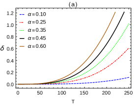
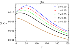
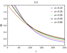
Figure 1: Mpemba effect in a qubit system under the action of thermal environment. The computations are performed for various values of $\alpha$ (which corresponds to different initial states) and the parameter $\gamma=0.01$. (a) The figure at the top illustrates the tightness of the bound 5. (b) The figure at the bottom left illustrates the time-averaged speed of evolution of the qubit system. (c) The figure at the bottom right illustrates the distance between different non-equilibrium states and the steady state, i.e., $\Theta(\rho_{ss},\rho_{T})$.

Let the initial state of the system be $\rho_{0}=\outerproduct{\psi}{\psi}$, where $\ket{\psi}=\alpha\ket{0}+\sqrt{1-\alpha^{2}}\ket{1}$. The state of the system at time $t$, evolving under the dynamical equation (Family of Exact and Inexact Quantum Speed Limits for Completely Positive and Trace-Preserving Dynamics), is $\rho_{t}=(1+\left(\alpha^{2}-1\right)e^{-t\gamma})\outerproduct{0}{0}+e^{-\frac{1}{2}t\gamma}\alpha\sqrt{1-\alpha^{2}}(\outerproduct{0}{1}+\outerproduct{1}{0})+\left(1-\alpha^{2}\right)e^{-t\gamma}\outerproduct{1}{1}$. The distance between the initial and time-evolved sate, $\Theta(\rho_{0},\rho_{t})$, is given by

$$\arccos\left(\frac{e^{-\gamma t}\left(2\alpha^{4}\left(1-e^{\frac{\gamma t}{2}}\right)+\alpha^{2}f(t,\gamma)+1\right)}{\sqrt{1-2\eta^{2}e^{-2\gamma t}\left(e^{\gamma t}-1\right)}}\right),$$ (22)

where $f(t,\gamma):=\left(2e^{\frac{\gamma t}{2}}+e^{\gamma t}-3\right)$ and $\eta:=1-\alpha^{2}$. For the bath at zero temperature, the steady state of the system is $\rho_{ss}=\outerproduct{0}{0}~{}(\alpha=1)$. Hence, the distance between the steady state and time-evolved state, $\Theta(\rho_{ss},\rho_{t})$, is given by

$$\arccos{\left(\frac{e^{\gamma t}-\eta}{\sqrt{2\eta^{2}(1-e^{\gamma t})+e^{2\gamma t}}}\right)}.$$

The speed of evolution of the qubit system under the thermal environment is given by

$$\Delta\mathcal{L}=\frac{\gamma e^{\frac{\gamma t}{2}}\sqrt{\eta\left(\alpha^{2}\left(2\eta^{2}+e^{2\gamma t}\right)+2\eta\left(\alpha^{2}+1\right)e^{\gamma t}\right)}}{\sqrt{2}\left(2\eta^{2}(1-e^{\gamma t})+e^{2\gamma t}\right)},$$ (23)

where $\mathcal{L}$ is the Liouvillian corresponding to Eq. (Family of Exact and Inexact Quantum Speed Limits for Completely Positive and Trace-Preserving Dynamics) and $\Delta\mathcal{L}$ is its variance in the state $|\tilde{\rho}_{t})$. The distance between an arbitrary pure initial state and the steady state is $\Theta(\rho_{0},\rho_{ss})=\arccos(\alpha^{2})$, which is a monotonically decreasing function of $\alpha$. The offset between the actual time of evolution and the speed limit time is defined as $\delta:=T-T_{QSL}$, where $T_{QSL}$ is the lower bound in Eq. (5). Here, $\delta$ measures the tightness of the bound 5. It is evident from Fig-1(a) that for considered far away non-equilibrium states (small $\alpha$) the generalized Mandelstam-Tamm bound is tighter than the closer non-equilibrium states (large $\alpha$). Hence, the considered far away non-equilibrium states relax faster than the closer non-equilibrium states because the far away non-equilibrium states take a shorter path (relatively close to geodesic) and evolve with higher average speed than the closer non-equilibrium states, as shown in Fig-1(b). As a result, the distance $\Theta(\rho_{ss},\rho_{T})$ between the far away non-equilibrium states and the steady state decreases much faster than that between the closer non-equilibrium states and the steady state, as shown in Fig-1(c), which is the so-called Mpemba effect.

Discussion and Conclusion: In this work, we have addressed the problem of the attainability of quantum speed limits for completely positive and trace-preserving (CPTP) dynamics. We have derived exact and inexact quantum speed limits for CPTP dynamics for finite-dimensional quantum systems in Liouville space. The exact and inexact speed limits are a consequence of the exact and inexact uncertainty relations for superoperators, respectively. The inexact speed limit saturates for time-optimal (fastest) CPTP dynamics, whereas the exact speed limit is exact for all CPTP dynamics and all states. We have characterized the fastest (time-optimal) CPTP dynamics and obtained its Liouvillian for given initial and orthogonal final states. Moreover, we have identified a key reason why the inexact speed limit is not attainable for non-time-optimal CPTP dynamics. The non-classical part of the generator (that does not commute with the initial state) solely drives this distinguishability and strongly depends on the initial and time-evolved states of the given quantum system. We have provided the geometrical interpretation of the exact and inexact speed limits using the geometry of quantum evolution in Liouville space. Moreover, we showed that the exact and inexact speed limits can be regarded as the exact and inexact generalization of the Mandelstam-Tamm bound as they provide exact and inexact time-energy-dissipation uncertainty relations. They suggest that fluctuations in energy and dissipation are responsible for the transportation of the state in the Liouville space. Moreover, we have also presented inexact speed limits for CPTP dynamics in terms of the Kraus operators and for arbitrary time-continuous dynamics beyond CPTP (see Appendix C).

We have provided two important applications of our bounds. First, we have shown that the speed of evolution bounds the growth of spectral form factor and Krylov complexity of states, which can have useful applications in many-body physics. Second, using the geometry of quantum evolution in Liouville space, particularly the tightness of inexact speed limits, we have successfully explained the counter-intuitive phenomena of the Mpemba effect in non-equilibrium open quantum dynamics. Our results significantly enhance our understanding of the relationship between time, energy, and dissipation in open quantum dynamics. Since the exact and inexact quantum speed limits have been derived from fundamentally well-established concepts such as uncertainty relations, non-commutativity, and the geometry of quantum evolution, we believe they can be verified in future experiments.

Previous studies suggest that there is a natural trade-off between the tightness of quantum speed limit and its computational complexity. However, we have transcended this trade-off as our speed limits are significantly simpler to compute than previously obtained speed limits as we are only required to estimate the overlap of density matrices and the variance of Liouvillian. Moreover, also these two quantities are experimentally easier to measure in the existing experimental platforms. We expect that our speed limits may have numerous applications in the rapidly growing field of quantum technologies including quantum computation, controlling and engineering dissipative processes, quantum metrology, and quantum energy storage and thermal devices, etc. The ideas presented in this article open the door to finding the exact or tight speed limits for other physical quantities of interest. Moreover, we have also derived the uncertainty relations for superoperators for the first time, which can have many applications in the future.

Appendix

Here, we include detailed preliminaries, derivations, and calculations to supplement the results presented in the main text.

Appendix A Preliminaries, Notations, Inequalities, and Equalities Used in the Main Text

Liouville space: For any quantum system of dimension $d$, there exists an associated Hilbert space $\mathsf{H}_{d}$. Let $\mathbb{B}(\mathsf{H}_{d})$ denote the set of all linear operators acting on $\mathsf{H}_{d}$. There is an isomorphism between $\mathbb{B}(\mathsf{H}_{d})$ and $\mathsf{H}_{d}\otimes\mathsf{H}_{d}$. Using this isomorphism, we can vectorize an arbitrary linear operator $A\in\mathbb{B}(\mathsf{H}_{d})$ as follows:

$$A=\sum_{ij}\alpha_{ij}\outerproduct{i}{j}~{}~{}\rightarrow~{}~{}|A)=\sum_{ij}\alpha_{ij}\ket{j}\otimes\ket{i}=\sum_{ij}\alpha_{ij}|ji),$$

where $\{\ket{i}\}$ forms an orthonormal basis for $\mathsf{H}_{d}$. The space of vectorized linear operators $\{|A)\}$ is called Liouville space (doubled Hilbert space), which is of dimension $d^{2}$ [53]. The Liouville space is equipped with an inner product given by $(A|B):=\operatorname{tr}(A^{{\dagger}}B)$. The state of a quantum system is represented by a linear positive semidefinite operator $\rho$ with a unit trace called the density matrix. The vectorized form of any density matrix $\rho$ is given by

$$\rho=\sum_{ij}\rho_{ij}\outerproduct{i}{j}\quad\rightarrow\quad|\rho)=\sum_{ij}\rho_{ij}|ji).$$

Note that $(\rho|\rho)=\operatorname{tr}(\rho^{2})\neq 1$ in general, hence we can define the corresponding normalized vector as $|\tilde{\rho})=\frac{|\rho)}{\sqrt{\operatorname{tr}(\rho^{2})}}$.

Liouville space angle: The shortest distance between two density matrices, $\rho_{a}$ and $\rho_{b}$, in Liouville space is defined as follows:

$$\Theta(\rho_{a},\rho_{b}):=\arccos{\left(\tilde{\rho}_{a}|\tilde{\rho}_{b}\right)},\hskip 8.5359pt\text{with}\hskip 8.5359pt(\tilde{\rho}_{a}|\tilde{\rho}_{b}):=\frac{\operatorname{tr}(\rho_{a}\rho_{b})}{\sqrt{\operatorname{tr}(\rho_{a}^{2})\operatorname{tr}(\rho_{b}^{2})}},$$ (24)

where $\Theta(\rho_{a},\rho_{b})$ is the Liouville space angle between state vectors $|\tilde{\rho}_{a})$ and $|\tilde{\rho}_{b})$. $\Theta(\rho_{a},\rho_{b})$ can be thought of as an analog of the Hilbert space angle between state vectors. It satisfies all the properties required for a valid distance measure:

1. Positive semidefinite: $\Theta(\rho_{a},\rho_{b})\geq 0$ for all $\rho_{a}$ and $\rho_{b}$.

2. Symmetric: $\Theta(\rho_{a},\rho_{b})=\Theta(\rho_{p},\rho_{a})$ for all $\rho_{a}$ and $\rho_{b}$.

3. Triangle inequality: $\Theta(\rho_{a},\rho_{b})\leq\Theta(\rho_{a},\rho_{c})+\Theta(\rho_{c},\rho_{b})$ for all $\rho_{a}$, $\rho_{b}$ and $\rho_{c}$.

Superoperator space: The linear operators that act on the vectors in the Liouville space are called superoperators, which we denote by $\mathcal{A},\mathcal{B},\ldots$, etc. These superoperators form a linear space equipped with an inner product $\langle\mathcal{A},\mathcal{B}\rangle:=\operatorname{tr}\left(\mathcal{A}^{{\dagger}}\mathcal{B}\right)$. The expectation value and the variance of the superoperator $\mathcal{O}$ in the state vector $|\tilde{\rho})$ is defined as:

$$(\!(\mathcal{O})\!) :=(\tilde{\rho}|\mathcal{O}|\tilde{\rho})=\operatorname{tr}(\mathcal{O}\mathcal{P})\quad\text{and}\quad(\Delta\mathcal{O})^{2}=\operatorname{tr}(\mathcal{O}^{\dagger}\mathcal{O}\mathcal{P})-\operatorname{tr}(\mathcal{O}^{\dagger}\mathcal{P})\operatorname{tr}(\mathcal{O}\mathcal{P}),$$

where $\mathcal{P}=|\tilde{\rho})(\tilde{\rho}|$ is the projection superoperator associated with the state vector $|\tilde{\rho})$.

Uncertainty relation for non-Hermitian superoperators (Proposition 1): For any two non-Hermitian superoperators $\mathcal{A}$ and $\mathcal{B}$, the following uncertainty relation holds:

$$(\Delta\mathcal{A})^{2}(\Delta\mathcal{B})^{2}\geq\left|\operatorname{tr}(\mathcal{A}^{\dagger}\mathcal{B}\mathcal{P})-\operatorname{tr}(\mathcal{A}^{\dagger}\mathcal{P})\operatorname{tr}(\mathcal{B}\mathcal{P})\right|^{2},$$ (25)

where $(\Delta\mathcal{O})^{2}=\operatorname{tr}(\mathcal{O}^{\dagger}\mathcal{O}\mathcal{P})-\operatorname{tr}(\mathcal{O}^{\dagger}\mathcal{P})\operatorname{tr}(\mathcal{O}\mathcal{P})$ is the variance of the superoperator $\mathcal{O}$ in the state vector $|\tilde{\rho})$.

Proof.

Let us define two vectors in the Liouville space as $|f):=(\mathcal{A}-\operatorname{tr}(\mathcal{A}\mathcal{P}))|\tilde{\rho})$ and $|g):=(\mathcal{B}-\operatorname{tr}(\mathcal{B}\mathcal{P}))|\tilde{\rho})$, where $\mathcal{A}$ and $\mathcal{B}$ are superoperators and $|\tilde{\rho})$ is a normalized vector in the Liouville space. Note that the inner product between the vectors $|A)$ and $|B)$ in the Liouville space is defined as $(A|B):=\operatorname{tr}{(A^{{\dagger}}B)}$. Thus, the inequalities that hold for inner product spaces must also exist in the Liouville space. Utilizing the Cauchy-Schwarz inequality, we obtain

$$(f|f)(g|g)\geq\absolutevalue{(f|g)}^{2}.$$ (26)

Now, by the definitions of $|f)$ and $|g)$, we have $(f|f)=\Delta\mathcal{A}^{2}$ and $(g|g)=\Delta\mathcal{B}^{2}$. Using these relations in the above inequality, we obtain $(\Delta\mathcal{A})^{2}(\Delta\mathcal{B})^{2}\geq\absolutevalue{\operatorname{tr}(\mathcal{A}^{\dagger}\mathcal{B}\mathcal{P})-\operatorname{tr}(\mathcal{A}^{\dagger}\mathcal{P})\operatorname{tr}(\mathcal{B}\mathcal{P})}^{2}$, which completes the proof. ∎

Important to note that in Eq. (25), if we replace the superoperators $\mathcal{A}$, $\mathcal{B}$, $\mathcal{P}$ by operators $A$, $B$, $\rho$ (density matrix), respectively, we retrieve the uncertainty relation for non-Hermitian operators obtained in the Ref. [63], which has recently been experimentally verified [64].

Exact uncertainty relation for superoperators (Proposition 2): For any Hermitian superoperator $\mathcal{A}=\sum_{i}a_{i}|a_{i})(a_{i}|$ and a non-Hermitian superoperator $\mathcal{B}$ there exists an exact uncertainty relation for all state vectors $|\tilde{\rho})$ as

$$\delta_{\mathcal{B}}\mathcal{A}\Delta\mathcal{B}_{\mathrm{n}c}=1/2,$$ (27)

where

$$(\delta_{\mathcal{B}}\mathcal{A})^{-2}:=\sum_{i}\frac{(a_{i}|(\mathcal{B}\mathcal{P}+\mathcal{P}\mathcal{B}^{\dagger}-\mathcal{P}\operatorname{tr}[\mathcal{P}(\mathcal{B}+\mathcal{B}^{\dagger})])|a_{i})^{2}}{(a_{i}|\mathcal{P}|a_{i})},~{}~{}\mathcal{B}=\mathcal{B}_{\mathrm{c}l}+\mathcal{B}_{\mathrm{n}c}~{}~{}\text{and}~{}~{}\mathcal{B}_{\mathrm{c}l}:=\sum_{i}|a_{i})(a_{i}|\frac{(a_{i}|\frac{1}{2}(\mathcal{B}\mathcal{P}-\mathcal{P}\mathcal{B}^{\dagger})|a_{i})}{(a_{i}|\mathcal{P}|a_{i})}.$$

Proof.

Given a Hermitian superoperator $\mathcal{A}$, we can always decompose a non-Hermitian superoperator $\mathcal{B}$ as a sum of two superoperators as $\mathcal{B}=\mathcal{B}_{\mathrm{c}l}+\mathcal{B}_{\mathrm{n}c}$, where $\mathcal{B}_{\mathrm{c}l}$ is anti-Hermitian and is diagonal in the eigenbasis of $\mathcal{A}$, and $\mathcal{B}_{\mathrm{n}c}$ is a non-Hermitian superoperator. The superoperator $\mathcal{B}_{\mathrm{c}l}$ is defined as

$$\mathcal{B}_{\mathrm{c}l}:=\sum_{i}|a_{i})(a_{i}|\frac{(a_{i}|\frac{1}{2}(\mathcal{B}\mathcal{P}-\mathcal{P}\mathcal{B}^{\dagger})|a_{i})}{(a_{i}|\mathcal{P}|a_{i})},$$ (28)

where $\{|a_{i})\}$ is the eigenbasis of $\mathcal{A}$. Then the variance of the non-classical part $\mathcal{B}_{\mathrm{n}c}$ in the state $|\tilde{\rho})$ is given by

$$\Delta\mathcal{B}_{\mathrm{n}c}^{2} = \Delta(\mathcal{B}-\mathcal{B}_{\mathrm{c}l})^{2}$$ (29)

$$= \operatorname{tr}(\mathcal{P}(\mathcal{B}-\mathcal{B}_{\mathrm{c}l})^{\dagger}(\mathcal{B}-\mathcal{B}_{\mathrm{c}l}))-\operatorname{tr}(\mathcal{P}(\mathcal{B}-\mathcal{B}_{\mathrm{c}l})^{\dagger})\operatorname{tr}(\mathcal{P}(\mathcal{B}-\mathcal{B}_{\mathrm{c}l})).$$

Let us consider the first term of the R.H.S. of the above equation

$$\operatorname{tr}(\mathcal{P}(\mathcal{B}-\mathcal{B}_{\mathrm{c}l})^{\dagger}(\mathcal{B}-\mathcal{B}_{\mathrm{c}l})) = \operatorname{tr}(\mathcal{P}\mathcal{B}^{\dagger}B-\mathcal{P}\mathcal{B}_{\mathrm{c}l}^{\dagger}B-\mathcal{P}\mathcal{B}^{\dagger}\mathcal{B}_{\mathrm{c}l}+\mathcal{P}\mathcal{B}_{\mathrm{c}l}^{\dagger}\mathcal{B}_{\mathrm{c}l})\pm\operatorname{tr}(\mathcal{P}\mathcal{B}_{\mathrm{c}l}^{\dagger}\mathcal{B}_{\mathrm{c}l})$$ (30)

$$= \operatorname{tr}(\mathcal{P}\mathcal{B}^{\dagger}B)-\operatorname{tr}(\mathcal{P}\mathcal{B}_{\mathrm{c}l}^{\dagger}\mathcal{B}_{\mathrm{c}l})+2\operatorname{tr}(\mathcal{P}\mathcal{B}_{\mathrm{c}l}^{\dagger}\mathcal{B}_{\mathrm{c}l})-\operatorname{tr}(\mathcal{B}_{\mathrm{c}l}\mathcal{P}\mathcal{B}^{\dagger}+\mathcal{B}_{\mathrm{c}l}^{\dagger}\mathcal{B}\mathcal{P})$$

$$= \operatorname{tr}(\mathcal{P}\mathcal{B}^{\dagger}B)-\operatorname{tr}(\mathcal{P}\mathcal{B}_{\mathrm{c}l}^{\dagger}\mathcal{B}_{\mathrm{c}l})-\sum_{i}\frac{(a_{i}|(\mathcal{B}\mathcal{P}-\mathcal{P}\mathcal{B}^{\dagger})|a_{i})^{2}}{2}+\sum_{i}\frac{(a_{i}|(\mathcal{B}\mathcal{P}-\mathcal{P}\mathcal{B}^{\dagger})|a_{i})^{2}}{2}$$

$$= \operatorname{tr}(\mathcal{P}\mathcal{B}^{\dagger}B)-\operatorname{tr}(\mathcal{P}\mathcal{B}_{\mathrm{c}l}^{\dagger}\mathcal{B}_{\mathrm{c}l}),$$

where to get the third equality, we used the definition of $\mathcal{B}_{\mathrm{c}l}$ from Eq. (28). Similarly, we can simplify the second term in Eq. (29)

$$\operatorname{tr}(\mathcal{P}(\mathcal{B}-\mathcal{B}_{\mathrm{c}l})^{\dagger})\operatorname{tr}(\mathcal{P}(\mathcal{B}-\mathcal{B}_{\mathrm{c}l})) = \operatorname{tr}(\mathcal{P}\mathcal{B}^{\dagger})\operatorname{tr}(\mathcal{P}\mathcal{B})-\operatorname{tr}(\mathcal{P}\mathcal{B}^{\dagger})\operatorname{tr}(\mathcal{P}\mathcal{B}_{\mathrm{c}l})-\operatorname{tr}(\mathcal{P}\mathcal{B}_{\mathrm{c}l}^{\dagger})\operatorname{tr}(\mathcal{P}\mathcal{B})+\operatorname{tr}(\mathcal{P}\mathcal{B}_{\mathrm{c}l}^{\dagger})\operatorname{tr}(\mathcal{P}\mathcal{B}_{\mathrm{c}l})$$ (31)

$$= \operatorname{tr}(\mathcal{P}\mathcal{B}^{\dagger})\operatorname{tr}(\mathcal{P}\mathcal{B})-\operatorname{tr}(\mathcal{P}\mathcal{B}_{\mathrm{c}l}^{\dagger})\operatorname{tr}(\mathcal{P}\mathcal{B}_{\mathrm{c}l})+\operatorname{tr}(\mathcal{P}\mathcal{B}_{\mathrm{c}l})\left(-2\operatorname{tr}(\mathcal{P}\mathcal{B}_{\mathrm{c}l})-\operatorname{tr}(\mathcal{P}\mathcal{B}^{\dagger})+\operatorname{tr}(\mathcal{P}\mathcal{B})\right)$$

$$= \operatorname{tr}(\mathcal{P}\mathcal{B}^{\dagger})\operatorname{tr}(\mathcal{P}\mathcal{B})-\operatorname{tr}(\mathcal{P}\mathcal{B}_{\mathrm{c}l}^{\dagger})\operatorname{tr}(\mathcal{P}\mathcal{B}_{\mathrm{c}l}),$$

where in the second equality we have added and subtracted $\operatorname{tr}(\mathcal{P}\mathcal{B}_{\mathrm{c}l}^{\dagger})\operatorname{tr}(\mathcal{P}\mathcal{B}_{\mathrm{c}l})$ on the R.H.S. of the equation and used the anti-Hermiticity $\mathcal{B}_{\mathrm{c}l}^{\dagger}=-\mathcal{B}_{\mathrm{c}l}$ to simplify its last term. Finally to get the last equality we have used the fact that $\operatorname{tr}(\mathcal{P}\mathcal{B}_{\mathrm{c}l})=1/2(\operatorname{tr}(\mathcal{P}\mathcal{B})-\operatorname{tr}(\mathcal{P}\mathcal{B}^{\dagger}))$ (see Eq. (28)). Thus using Eqs. (30) and (31) in Eq. (29), we obtain

$$\Delta\mathcal{B}_{\mathrm{n}c}^{2} = \Delta\mathcal{B}^{2}-\Delta\mathcal{B}_{\mathrm{c}l}^{2}$$ (32)

$$= \operatorname{tr}(\mathcal{B}^{\dagger}\mathcal{B}\mathcal{P})-\operatorname{tr}(\mathcal{B}^{\dagger}\mathcal{P})\operatorname{tr}(\mathcal{B}\mathcal{P})-\operatorname{tr}(\mathcal{B}_{\mathrm{c}l}^{\dagger}\mathcal{B}_{\mathrm{c}l}\mathcal{P})+\operatorname{tr}(\mathcal{B}_{\mathrm{c}l}^{\dagger}\mathcal{P})\operatorname{tr}(\mathcal{B}_{\mathrm{c}l}\mathcal{P})$$

$$= \frac{1}{4}\left[\sum_{i}\left((a_{i}|\mathcal{B}|\tilde{\rho})^{2}+(\tilde{\rho}|\mathcal{B}^{\dagger}|a_{i})^{2}\right)-\left(\operatorname{tr}(\mathcal{B}\mathcal{P})+\operatorname{tr}(\mathcal{B}^{\dagger}\mathcal{P})\right)^{2}+2\operatorname{tr}(\mathcal{B}^{\dagger}\mathcal{B}\mathcal{P})\right].$$

Let us now define a measure of uncertainty for the superoperator $\mathcal{A}$, denoted by $\delta_{\mathcal{B}}\mathcal{A}$, as

$$(\delta_{\mathcal{B}}\mathcal{A})^{-2}=\sum_{i}\frac{(a_{i}|(\mathcal{B}\mathcal{P}+\mathcal{P}\mathcal{B}^{\dagger}-\mathcal{P}\operatorname{tr}[\mathcal{P}(\mathcal{B}+\mathcal{B}^{\dagger})])|a_{i})^{2}}{(a_{i}|\mathcal{P}|a_{i})}.$$

For $\mathcal{P}=|\tilde{\rho})(\tilde{\rho}|$, the above equation can be rewritten as

$$(\delta_{\mathcal{B}}\mathcal{A})^{-2}=\left[\sum_{i}\left((a_{i}|\mathcal{B}|\tilde{\rho})^{2}+(\tilde{\rho}|\mathcal{B}^{\dagger}|a_{i})^{2}\right)-\left(\operatorname{tr}(\mathcal{B}\mathcal{P})+\operatorname{tr}(\mathcal{B}^{\dagger}\mathcal{P})\right)^{2}+2\operatorname{tr}(\mathcal{B}^{\dagger}\mathcal{B}\mathcal{P})\right].$$ (33)

Finally, using Eqs. (32) and (33), we obtain

$$\delta_{\mathcal{B}}\mathcal{A}\Delta\mathcal{B}_{\mathrm{n}c}=1/2,$$ (34)

which holds for an arbitrary state vector $|\tilde{\rho})$ corresponding to the density matrix $\rho$. It is important to note that $\mathcal{B}_{\mathrm{c}l}$ commutes with $\mathcal{A}$, whereas $\mathcal{B}_{\mathrm{n}c}$ does not commute with $\mathcal{A}$, and the exact uncertainty relation is based on the non-commutativity of the given two superoperators. ∎

Interestingly, in Eq. (27), if we replace the superoperators $\mathcal{A}$, $\mathcal{B}$, and $\mathcal{P}$ with the operators $A$, $B$, and $\rho$ (density matrix), respectively, we obtain the exact uncertainty relation for two operators $A$ and $B$ (where $A$ is Hermitian and $B$ is non-Hermitian). This result reduces to the exact uncertainty relation obtained by M.J. Hall in Ref. [65] if both operators are Hermitian and $\rho$ is a pure state.

Dynamical equation for CPTP dynamics: Here, we consider the physical processes which are described by completely positive and trace-preserving (CPTP) dynamics. For finite-dimensional systems, any CPTP dynamics can be described by a time-local master equation which can be written as [66, 67, 61]:

$$\frac{d\rho_{t}}{dt}=\mathbb{L}_{t}(\rho_{t})=-i[H_{t},\rho_{t}]+\sum_{k=1}^{d^{2}-1}\gamma^{k}_{t}\left(L^{k}_{t}\rho_{t}L^{k\dagger}_{t}-\frac{1}{2}\{L^{k\dagger}_{t}L^{k}_{t},\rho_{t}\}\right),$$ (35)

where $H_{t}$ is the driving Hamiltonian of the system and $L^{k}_{t}$ are the Lindblad operators with rates $\gamma^{k}_{t}$. If $\gamma^{k}_{t}\geq 0$ the corresponding dynamical map $\Lambda_{t}=\mathcal{T}\exp\left(\int_{0}^{t}d\tau\mathbb{L}_{\tau}\right)$ is completely positive and divisible, where $\mathcal{T}$ is the time ordering operator. However, when the Hamiltonian, Lindblad operators, and the rates are time-independent, the map can be written as $\Lambda_{t}=\exp\left(\mathbb{L}t\right)$ [61, 68, 69]. It is important to note that there may exist a CPTP dynamical map $\Lambda_{t}$ that cannot be expressed in the form of a Lindblad master equation.

Recall that for the product of three operators $A,B$ and $C$ the following identity holds [53]:

$$|ABC)=(C^{T}\otimes A)|B),$$ (36)

where $C^{T}$ is the transpose of $C$.

The vectorized form of the above master equation can be written as

$$\frac{d}{dt}|\rho_{t})=\mathcal{L}_{t}|\rho_{t}),$$ (37)

where $\mathcal{L}_{t}$ is called Liouvillian superoperator which can be written using Eqs. (36) and (35) as follows

$$|[H_{t},\rho_{t}]) = |H_{t}\rho_{t}\mathbb{I})-|\mathbb{I}\rho_{t}H_{t})=\left(\mathbb{I}\otimes H_{t}-H_{t}^{T}\otimes\mathbb{I}\right)|\rho_{t}),$$

$$|L^{k}_{t}\rho_{t}L^{k\dagger}_{t})-\frac{1}{2}|\{L^{k\dagger}_{t}L^{k}_{t},\rho_{t}\}) = \left(L^{k*}_{t}\otimes L^{k}_{t}-\frac{1}{2}\left(\mathbb{I}\otimes L^{k\dagger}_{t}L^{k}_{t}+(L^{k\dagger}_{t}L^{k}_{t})^{T}\otimes\mathbb{I}\right)\right)|\rho_{t}),$$ (38)

where $\mathbb{I}$ is the identity operator. Using the above two equations, we obtain

$$\mathcal{L}_{t} = -i\mathcal{L}_{H}+\mathcal{L}_{D},$$ (39)

where $\mathcal{L}_{H}:=\left(\mathbb{I}\otimes H_{t}-H_{t}^{T}\otimes\mathbb{I}\right)$ is Hermitian and is the generator of the unitary dynamics, and $\mathcal{L}_{D}:=\sum_{k}\gamma_{k}\left(L^{k*}_{t}\otimes L^{k}_{t}-\frac{1}{2}\left(\mathbb{I}\otimes L^{k\dagger}_{t}L^{k}_{t}+(L^{k\dagger}_{t}L^{k}_{t})^{T}\otimes\mathbb{I}\right)\right)$ is non-Hermitian and is the generator of the dissipative dynamics.

The above master Eq. (37) does not preserve the norm of the state; therefore, the norm preserving master equation for any normalized state $|\tilde{\rho}_{t})$ can be written as

$$\frac{d}{dt}|\tilde{\rho}_{t}) = \frac{d}{dt}\left(\frac{|\rho_{t})}{\sqrt{(\rho_{t}|\rho_{t})}}\right)=\frac{d}{dt}|{\tilde{\rho}_{t}})=(\mathcal{L}_{t}-\frac{1}{2}\{(\tilde{\rho}_{t}|\mathcal{L}_{t}|\tilde{\rho}_{t})+(\tilde{\rho}_{t}|\mathcal{L}_{t}^{\dagger}|\tilde{\rho}_{t})\})|{\tilde{\rho}_{t}}),$$ (40)

where $|\tilde{\rho}_{t})=\frac{|\rho_{t})}{\sqrt{(\rho_{t}|\rho_{t})}}$ and $(\rho_{t}|\rho_{t})=\operatorname{tr}(\rho_{t}^{2})$. The above equation is valid for arbitrary Liouvillian. However, for the Lindblad master equation, we can further simplify the above equation by using the decomposition of $\mathcal{L}_{t}$ as $\mathcal{L}_{t}=-i\mathcal{L}_{H}+\mathcal{L}_{D}$, we have

$$(\tilde{\rho}_{t}|(\mathcal{L}_{t}-\mathcal{L}_{t}^{\dagger})|\tilde{\rho}_{t}) = (\tilde{\rho}_{t}|(-2i\mathcal{L}_{H}+\mathcal{L}_{D}-\mathcal{L}_{D}^{\dagger})|\tilde{\rho}_{t})$$ (41)

$$= -2i(\tilde{\rho}_{t}|\mathcal{L}_{H}|\tilde{\rho}_{t})+(\tilde{\rho}_{t}|\mathcal{L}_{D}|\tilde{\rho}_{t})-(\tilde{\rho}_{t}|\mathcal{L}_{D}^{\dagger}|\tilde{\rho}_{t})$$

$$= -2i(\tilde{\rho}_{t}|\left(\mathbb{I}\otimes H_{t}-H_{t}^{T}\otimes\mathbb{I}\right)|\tilde{\rho}_{t})+\sum_{k}\gamma^{k}(\tilde{\rho}_{t}|\left(L^{k*}_{t}\otimes L^{k}_{t}-\frac{1}{2}\left(\mathbb{I}\otimes L^{k\dagger}_{t}L^{k}_{t}+(L^{k\dagger}_{t}L^{k}_{t})^{T}\otimes\mathbb{I}\right)\right)|\tilde{\rho}_{t})$$

$$-\sum_{k}\gamma^{k}(\tilde{\rho}_{t}|\left(L^{k^{T}}_{t}\otimes L^{k\dagger}_{t}-\frac{1}{2}\left(\mathbb{I}\otimes L^{k\dagger}_{t}L^{k}_{t}+(L^{k\dagger}_{t}L^{k}_{t})^{*}\otimes\mathbb{I}\right)\right)|\tilde{\rho}_{t})$$

$$= -2i(\tilde{\rho}_{t}|[H_{t},\tilde{\rho}_{t}])+\sum_{k}\gamma^{k}(\tilde{\rho}_{t}|L_{t}^{k}\tilde{\rho}_{t}L_{t}^{k\dagger}-\frac{1}{2}\{L_{t}^{k\dagger}L_{t}^{k},\tilde{\rho}_{t}\})-\sum_{k}\gamma^{k}(\tilde{\rho}_{t}|L_{t}^{k\dagger}\tilde{\rho}_{t}L_{t}^{k}-\frac{1}{2}\{L_{t}^{k\dagger}L_{t}^{k},\tilde{\rho}_{t}\})$$

$$= -2i\operatorname{tr}(\tilde{\rho}_{t}[H_{t},\tilde{\rho}_{t}])+\sum_{k}\gamma^{k}\left(\operatorname{tr}(\tilde{\rho}_{t}L_{t}^{k}\tilde{\rho}_{t}L_{t}^{k\dagger})-\operatorname{tr}(\tilde{\rho}_{t}L_{t}^{k\dagger}\tilde{\rho}_{t}L_{t}^{k})\right)$$

$$= 0,$$

where the fourth equality is due to Eq. (A) and in the fifth equality, we have used the fact that $(A|B)=\operatorname{tr}(A^{\dagger}B)$. Finally, using the cyclic property of trace, we obtain the last equality. Hence, $(\tilde{\rho}_{t}|\mathcal{L}|\tilde{\rho}_{t})$ is a real number for any state $|\tilde{\rho}_{t})$, and thus for Lindblad master equation, Eq. (40) can be written as

$$\frac{d}{dt}|{\tilde{\rho}_{t}})=\left(\mathcal{L}_{t}-(\tilde{\rho}_{t}|\mathcal{L}_{t}|\tilde{\rho}_{t})\right)|\tilde{\rho}_{t}).$$ (42)

Using Eq. (40), the time evolution of the projection superoperator ${\mathcal{P}}_{t}=|\tilde{\rho}_{t})(\tilde{\rho}_{t}|$ associated with the time-evolved state vector $|\tilde{\rho}_{t})$ is given by the following master equation

$$\frac{d}{dt}\mathcal{P}_{t}=\mathcal{L}_{t}\mathcal{P}_{t}+\mathcal{P}_{t}\mathcal{L}_{t}^{\dagger}-\mathcal{P}_{t}\operatorname{tr}\left[(\mathcal{L}_{t}+\mathcal{L}_{t}^{\dagger})\mathcal{P}_{t}\right].$$ (43)

The Liouvillian superoperator can also be decomposed into an anti-Hermitian and a Hermitian part as $\mathcal{L}=-i\mathcal{L}_{+}+\mathcal{L}_{-}$, where $\mathcal{L}_{+}=\mathcal{L}_{H}+i\left(\mathcal{L}_{D}-\mathcal{L}^{\dagger}_{D}\right)/2$ and $\mathcal{L}_{-}=\left(\mathcal{L}_{D}+\mathcal{L}^{\dagger}_{D}\right)/2$ are associated with the reversible and irreversible parts of the dynamics, respectively.

Appendix B Detailed Proof of Theorem 1

Using Eq. (43), the rate of change of the distinguishability between the initial state vector $|\tilde{\rho}_{0})$ and the time-evolved state vector $|\tilde{\rho}_{t})$ is given by

$$\frac{d}{dt}(\tilde{\rho}_{0}|\tilde{\rho}_{t})^{2} = \frac{d}{dt}\operatorname{tr}(\mathcal{P}_{t}\mathcal{P}_{0})=\operatorname{tr}\left(\mathcal{L}\mathcal{P}_{t}\mathcal{P}_{0}\right)+\operatorname{tr}\left(\mathcal{P}_{t}\mathcal{L}^{\dagger}\mathcal{P}_{0}\right)-\operatorname{tr}\left(\mathcal{P}_{t}\mathcal{P}_{0}\right)\operatorname{tr}\left(\left(\mathcal{L}+\mathcal{L}^{\dagger}\right)\mathcal{P}_{t}\right)$$ (44)

$$= X+X^{*},$$ (45)

where $\mathcal{P}_{t}=|\tilde{\rho}_{t})(\tilde{\rho}_{t}|$ and $\mathcal{P}_{0}=|\tilde{\rho}_{0})(\tilde{\rho}_{0}|$ are the projection superoperators associated with the initial and time-evolved state vectors, respectively, $X:=\operatorname{tr}(\mathcal{L}\mathcal{P}_{t}\mathcal{P}_{0})-\operatorname{tr}(\mathcal{P}_{t}\mathcal{P}_{0})\operatorname{tr}(\mathcal{L}\mathcal{P}_{t})$ and $X^{*}$ is the complex conjugate of $X$. Let us take the absolute value of both sides of the above equation, then we obtain

$$\left|\frac{d}{dt}\operatorname{tr}(\mathcal{P}_{t}\mathcal{P}_{0})\right| = |X+X^{*}|$$ (46)

$$\leq 2|X|$$

$$= 2|\operatorname{tr}(\mathcal{L}\mathcal{P}_{t}\mathcal{P}_{0})-\operatorname{tr}(\mathcal{P}_{t}\mathcal{P}_{0})\operatorname{tr}(\mathcal{L}\mathcal{P}_{t})|,$$

where in the second step, we use the triangle inequality and the fact that $|X|=|X^{*}|$.

Using the uncertainty relation for non-Hermitian superoperators 25 ($\mathcal{A}=\mathcal{P}_{0}$ and $\mathcal{B}=\mathcal{L}$) and the above inequality, we obtain the following bound on the rate of change of the distinguishability

$$\left|\frac{d}{dt}\operatorname{tr}(\mathcal{P}_{t}\mathcal{P}_{0})\right|\leq 2|\operatorname{tr}(\mathcal{L}\mathcal{P}_{t}\mathcal{P}_{0})-\operatorname{tr}(\mathcal{P}_{t}\mathcal{P}_{0})\operatorname{tr}(\mathcal{L}\mathcal{P}_{t})|\leq 2\Delta\mathcal{L}\Delta\mathcal{P}_{0},$$ (47)

where $(\Delta\mathcal{O})^{2}=\operatorname{tr}(\mathcal{O}^{\dagger}\mathcal{O}\mathcal{P}_{t})-\operatorname{tr}(\mathcal{O}^{\dagger}\mathcal{P}_{t})\operatorname{tr}(\mathcal{O}\mathcal{P}_{t})$ is the variance of the superoperator $\mathcal{O}$ in the state $|\tilde{\rho}_{t})$. Let us integrate the above inequality on both sides and use the fact that $\absolutevalue{\int f(t)dt}\leq\int\absolutevalue{f(t)}dt$, then we obtain

$$\absolutevalue{\int_{0}^{T}\frac{d\operatorname{tr}(\mathcal{P}_{t}\mathcal{P}_{0})}{\sqrt{\operatorname{tr}(\mathcal{P}_{t}\mathcal{P}_{0})}\sqrt{1-\operatorname{tr}(\mathcal{P}_{t}\mathcal{P}_{0})}}}\leq 2\int_{0}^{T}\Delta\mathcal{L}dt.$$ (48)

On performing the above integration, we obtain the following lower bound on the evolution time

$$T\geq\frac{\Theta(\rho_{0},\rho_{T})}{\langle\!\langle\Delta\mathcal{L}\rangle\!\rangle_{T}},$$ (49)

where ${\Theta(\rho_{0},\rho_{T})}=\arccos(\tilde{\rho}_{0}|\tilde{\rho}_{T})$ is the Liouville space angle between the initial state vector $|\tilde{\rho}_{0})$ and the final state vector $|\tilde{\rho}_{T})$, and ${\langle\!\langle\Delta\mathcal{L}\rangle\!\rangle_{T}}=\frac{1}{T}\int_{0}^{T}\,dt\Delta\mathcal{L}$. Furthermore, we can write the variance of the Liouvillian as follows

$$\Delta\mathcal{L}^{2} = {\operatorname{tr}(\mathcal{L}^{\dagger}\mathcal{L}\mathcal{P}_{t})-\operatorname{tr}(\mathcal{L}\mathcal{P}_{t})^{2}}$$ (50)

$$= {\operatorname{tr}\left((i\mathcal{L}_{H}+\mathcal{L}_{D}^{\dagger})(-i\mathcal{L}_{H}+\mathcal{L}_{D})\mathcal{P}_{t}\right)-\operatorname{tr}\Big{(}(-i\mathcal{L}_{H}+\mathcal{L}_{D})\mathcal{P}_{t}\Big{)}^{2}}$$

$$= {\operatorname{tr}(\mathcal{L}_{H}^{2}\mathcal{P}_{t})+i\operatorname{tr}\left((\mathcal{L}_{H}\mathcal{L}_{D}-\mathcal{L}_{D}^{\dagger}\mathcal{L}_{H})\mathcal{P}_{t}\right)+\operatorname{tr}(\mathcal{L}_{D}^{\dagger}\mathcal{L}_{D}\mathcal{P}_{t})-\operatorname{tr}(\mathcal{L}_{D}\mathcal{P}_{t})^{2}}$$

$$= {\Delta\mathcal{L}_{H}^{2}+\Delta\mathcal{L}_{D}^{2}+i\operatorname{tr}\left((\mathcal{L}_{H}\mathcal{L}_{D}-\mathcal{L}_{D}^{\dagger}\mathcal{L}_{H})\mathcal{P}_{t}\right)},$$

where in the second equality, we have used the decomposition $\mathcal{L}=-i\mathcal{L}_{H}+\mathcal{L}_{D}$, and the third equality is due to the fact that $\operatorname{tr}(\mathcal{L}_{H}\mathcal{P}_{t})=0$ (see Eq. (41)). Here, $\Delta\mathcal{L}_{H}^{2}=\frac{2}{\operatorname{tr}{(\rho_{t}^{2})}}\left(\operatorname{tr}\left(\rho_{t}^{2}H_{t}^{2}\right)-\operatorname{tr}\left(\rho_{t}H_{t}\rho_{t}H_{t}\right)\right)$, which reduces to the variance of the Hamiltonian if $\rho_{t}$ is a pure state. Moreover, the last term of the above equation is upper bounded by $2\Delta\mathcal{L}_{H}\Delta\mathcal{L}_{D}$. To see this, let us define two vectors $|a):=\left(\mathcal{L}_{H}-\operatorname{tr}\left(\mathcal{L}_{H}\mathcal{P}_{t}\right)\right)|\tilde{\rho}_{t})$ and $|b):=\left(\mathcal{L}_{D}-\operatorname{tr}\left(\mathcal{L}_{D}\mathcal{P}_{t}\right)\right)|\tilde{\rho}_{t})$. Now using the Cauchy-Schwarz inequality for $|a)$ and $|b)$, we get:

$$(a|a)(b|b)\geq\absolutevalue{(a|b)}^{2}\geq\left(\frac{1}{2i}\left[(a|b)-(b|a)\right]\right)^{2},$$ (51)

where in the last inequality we have used the fact that for any complex number $z$, we have $\absolutevalue{z}^{2}\geq(\mathrm{Im}(z))^{2}$. Now, by the definitions of $|a)$ and $|b)$, we have $(a|a)=\Delta\mathcal{L}^{2}_{H}$, $(g|g)=\Delta\mathcal{L}^{2}_{D}$, and $(a|b)-(b|a)=\operatorname{tr}\left((\mathcal{L}_{H}\mathcal{L}_{D}-\mathcal{L}_{D}^{\dagger}\mathcal{L}_{H})\mathcal{P}_{t}\right)$. Using these in the above equation, we obtain

$$2\Delta\mathcal{L}_{H}\Delta\mathcal{L}_{D}\geq i\operatorname{tr}\left((\mathcal{L}_{H}\mathcal{L}_{D}-\mathcal{L}_{D}^{\dagger}\mathcal{L}_{H})\mathcal{P}_{t}\right).$$ (52)

If we take the decomposition of the Liouvillian superoperator into an anti-Hermitian and a Hermitian part as $\mathcal{L}=-i\mathcal{L}_{+}+\mathcal{L}_{-}$, then we can write the variance of the Liouvillian as follows

$$\Delta\mathcal{L}^{2} = {\Delta\mathcal{L}_{+}^{2}+\Delta\mathcal{L}_{-}^{2}+i\operatorname{tr}\left(\left[\mathcal{L}_{+},\mathcal{L}_{-}\right]\mathcal{P}_{t}\right)}.$$ (53)

Appendix C Geometrical derivation of Inexact Quantum Speed Limit for arbitrary time-continuous dynamics

The Hilbert-Schmidt distance between two state vectors $|\tilde{\rho}_{1})$ and $|\tilde{\rho}_{2})$ is given as

$$S^{2}=\frac{1}{2}\norm{\mathcal{P}_{1}-\mathcal{P}_{2}}^{2}_{\mathrm{H}S}=(1-(\tilde{\rho}_{1}|\tilde{\rho}_{2})(\tilde{\rho}_{2}|\tilde{\rho}_{1})),$$ (54)

where $\mathcal{P}_{1}=|\tilde{\rho}_{1})(\tilde{\rho}_{1}|$ and $\mathcal{P}_{2}=|\tilde{\rho}_{2})(\tilde{\rho}_{2}|$ are superoperators associated with the state vectors $|\tilde{\rho}_{1})$ and $|\tilde{\rho}_{2})$, respectively.

Let us consider a quantum system whose evolution is governed by an arbitrary time-continuous dynamics. At time $t$, its state vector is given by $|\tilde{\rho}_{t})$. The distance between two infinitesimally separated state vectors $|\tilde{\rho}_{t})$ and $|\tilde{\rho}_{t+dt})$ is given as

$$dS^{2} = (1-(\tilde{\rho}_{t}|\tilde{\rho}_{t+dt})(\tilde{\rho}_{t+dt}|\tilde{\rho}_{t}))$$ (55)

$$= \left(1-\frac{(\rho_{t}|\rho_{t+dt})(\rho_{t+dt}|\rho_{t})}{(\rho_{t}|\rho_{t})(\rho_{t+dt}|\rho_{t+dt})}\right),$$

where $|\tilde{\rho}_{t})=|\rho_{t})/\sqrt{(\rho_{t}|\rho_{t})}$.

Using the Taylor expansion of $|\rho_{t+dt})$ and taking its inner product with $|\rho_{t})$, we obtain

$$(\rho_{t}|\rho_{t+dt})=(\rho_{t}|\rho_{t})+(\rho_{t}|\dot{\rho}_{t})dt+(\rho_{t}|\ddot{\rho}_{t})\frac{dt^{2}}{2}+{\text{higher order terms}}.$$ (56)

Using above expression, we can expand the quantity $(\rho_{t}|\rho_{t+dt})(\rho_{t+dt}|\rho_{t})$ up to second order in $dt$ as

$$(\rho_{t}|\rho_{t+dt})(\rho_{t+dt}|\rho_{t})=(\rho_{t}|\rho_{t})\left((\rho_{t}|\rho_{t})+\left((\dot{\rho}_{t}|\rho_{t})+(\rho_{t}|\dot{\rho}_{t})\right)dt+\left((\ddot{\rho}_{t}|\rho_{t})+2(\rho_{t}|\dot{\rho}_{t})(\dot{\rho}_{t}|\rho_{t})+(\rho_{t}|\ddot{\rho}_{t})\right)\frac{dt^{2}}{2}\right).$$ (57)

Similarly,

$$(\rho_{t+dt}|\rho_{t+dt})=(\rho_{t}|\rho_{t})+\left((\rho_{t}|\dot{\rho}_{t})+(\dot{\rho}_{t}|\rho_{t})\right)dt+\left((\rho_{t}|\ddot{\rho}_{t})+2(\dot{\rho}_{t}|\dot{\rho}_{t})+(\ddot{\rho}_{t}|\rho_{t})\right)\frac{dt^{2}}{2}.$$ (58)

Using the above two equations and considering the terms up to $dt^{2}$, we obtain the expression for $dS^{2}$ as follows

$$dS^{2} =\left(\frac{(\dot{\rho}_{t}|\dot{\rho}_{t})}{(\rho_{t}|\rho_{t})}-\frac{(\rho_{t}|\dot{\rho}_{t})(\dot{\rho}_{t}|\rho_{t})}{(\rho_{t}|\rho_{t})^{2}}\right)dt^{2}$$

$$=\left((\dot{\tilde{\rho}}_{t}|\dot{\tilde{\rho}}_{t})-(\tilde{\rho}_{t}|\dot{\tilde{\rho}}_{t})(\dot{\tilde{\rho}}_{t}|\tilde{\rho}_{t})\right)dt^{2},$$ (59)

where $|\dot{\tilde{\rho}}_{t})=\frac{d}{dt}|\tilde{\rho}_{t})$ and the second equality follows from the fact that

$$\frac{(\dot{\rho}_{t}|\dot{\rho}_{t})}{(\rho_{t}|\rho_{t})}=(\dot{\tilde{\rho}}_{t}|\dot{\tilde{\rho}}_{t})+\frac{((\dot{\rho}_{t}|\rho_{t})+(\rho_{t}|\dot{\rho}_{t}))^{2}}{4(\rho_{t}|\rho_{t})^{2}}~{}~{}\text{and}~{}~{}\frac{(\rho_{t}|\dot{\rho}_{t})(\dot{\rho}_{t}|\rho_{t})}{(\rho_{t}|\rho_{t})^{2}}=(\tilde{\rho}_{t}|\dot{\tilde{\rho}}_{t})(\dot{\tilde{\rho}}_{t}|\tilde{\rho}_{t})+\frac{((\dot{\rho}_{t}|\rho_{t})+(\rho_{t}|\dot{\rho}_{t}))^{2}}{4(\rho_{t}|\rho_{t})^{2}}.$$ (60)

The Eq. (C) can be thought of as Fubini-study metric in Liouville space, where $dS$ measures the elemental distance along the evolution path (trajectory). Using Eq. (C), the speed of the evolution (transportation) of the quantum system in Liouville space can be defined as

$$\mathcal{V}_{t}=\frac{dS}{dt}=\sqrt{(\dot{\tilde{\rho}}_{t}|\dot{\tilde{\rho}}_{t})-(\tilde{\rho}_{t}|\dot{\tilde{\rho}}_{t})(\dot{\tilde{\rho}}_{t}|\tilde{\rho}_{t})}.$$ (61)

On integrating the above equation, we obtain

$$T=\frac{S}{{\langle\!\langle\mathcal{V}_{t}\rangle\!\rangle_{T}}},~{}~{}~{}\text{where}~{}~{}{\langle\!\langle\mathcal{V}_{t}\rangle\!\rangle_{T}}=\frac{1}{T}\int_{0}^{T}dt~{}\mathcal{V}_{t}.$$ (62)

Now, using the geometry of quantum evolution in Liouville space, the total distance $S$ traveled by the state vector $|\tilde{\rho}_{t})$, along the evolution path which joins the state vectors $|\tilde{\rho}_{0})$ and $|\tilde{\rho}_{T})$ is always lower bounded by the shortest distance (geodesic) connecting them, i.e., $S\geq\Theta(\rho_{0},\rho_{T})$. Thus, we obtain a lower bound on the total evolution time of a quantum system

$$T\geq\frac{\Theta(\rho_{0},\rho_{T})}{{\langle\!\langle\mathcal{V}_{t}\rangle\!\rangle_{T}}}.$$ (63)

The above bound is applicable to arbitrary time-continuous dynamics. It is important to note that previously a geometric quantum speed limit has been obtained for arbitrary time-continuous dynamics, which requires purification of the states (see Ref. [28]). This approach may have some shortcomings because purifications can overestimate the distance between states, and also the speed of evolution. However, the bound (63) does not have such shortcomings; therefore, it is relatively better. Moreover, the bound (63) is significantly simpler to calculate than other geometric speed limits applicable to arbitrary time-continuous dynamics (see Refs. [45, 46]). It is not fair to compare the bound (63) with non-geometric quantum speed limits obtained using mathematical inequalities, such as the Cauchy-Schwarz and Hölder inequalities, because, in general, they are loose and arguably hard to compute as they require estimating the norms of non-Hermitian operators.

Geometrical derivation of Theorem -1 (Inexact Quantum Speed Limit for CPTP dynamics):— For the CPTP dynamics given by Eq. (40), we can write the speed of evolution as

$$\mathcal{V}_{t}=\Delta\mathcal{L}=\sqrt{\operatorname{tr}\left(\mathcal{L}^{\dagger}\mathcal{L}\mathcal{P}_{t}\right)-\operatorname{tr}\left(\mathcal{L}\mathcal{P}_{t}\right)\operatorname{tr}\left(\mathcal{L}^{\dagger}\mathcal{P}_{t}\right)}.$$ (64)

To arrive at Eq. (64) from Eq. (63), we have used $(\dot{\tilde{\rho}}_{t}|\dot{\tilde{\rho}}_{t})=\operatorname{tr}(\mathcal{L}^{\dagger}\mathcal{L}\mathcal{P}_{t})-(\operatorname{tr}\left(\mathcal{L}\mathcal{P}_{t}\right)+\operatorname{tr}(\mathcal{L}^{\dagger}\mathcal{P}_{t}))^{2}/4$ and $(\tilde{\rho}_{t}|\dot{\tilde{\rho}}_{t})(\dot{\tilde{\rho}}_{t}|\tilde{\rho}_{t})=\operatorname{tr}\left(\mathcal{L}\mathcal{P}_{t}\right)\operatorname{tr}(\mathcal{L}^{\dagger}\mathcal{P}_{t})-(\operatorname{tr}\left(\mathcal{L}\mathcal{P}_{t}\right)+\operatorname{tr}(\mathcal{L}^{\dagger}\mathcal{P}_{t}))^{2}/4$. Using this evolution speed in Eq. (63), we obtain

$$T\geq\frac{\Theta(\rho_{0},\rho_{T})}{\langle\!\langle\Delta\mathcal{L}\rangle\!\rangle_{T}},$$ (65)

where $\langle\!\langle\Delta\mathcal{L}\rangle\!\rangle_{T}=\frac{1}{T}\int_{0}^{T}dt\Delta\mathcal{L}$.

Geometrical derivation of Inexact Quantum Speed Limit for CPTP map described by operator-sum representation:— The CPTP dynamics of a quantum system can also be described by the operator-sum representation, which is given as:

$$\rho_{t}=\sum_{i}K_{i}(t)\rho_{0}K^{\dagger}_{i}(t),$$ (66)

where $\{K_{i}(t)\}$ are called Kraus operators and satisfy the completeness relation $\sum_{i}K_{i}^{{\dagger}}(t)K_{i}(t)=\mathbb{I}$. The vectorized form of the above equation can be written as $|\rho_{t})=\mathcal{K}_{t}|\rho_{0})$, where $\mathcal{K}_{t}=\sum_{i}K_{i}(t)\otimes K^{*}_{i}(t)$ is the corresponding superoperator that acts on $|\rho_{0})$ in the Liouville space. The normalized state evolves as $|\tilde{\rho}_{t})=\widetilde{\mathcal{K}}_{t}|\tilde{\rho}_{0})$, where $\widetilde{\mathcal{K}}_{t}=\mathcal{K}_{t}/\sqrt{(\rho_{0}\mathcal{K}^{\dagger}_{t}|\mathcal{K}_{t}\rho_{0})}$. Using this equation we obtain $(\dot{\tilde{\rho}}_{t}|\dot{\tilde{\rho}}_{t})=\operatorname{tr}(\dot{\widetilde{\mathcal{K}}}^{\dagger}_{t}\dot{\widetilde{\mathcal{K}}}_{t}\mathcal{P}_{0})$ and $(\tilde{\rho}_{t}|\dot{\tilde{\rho}}_{t})(\dot{\tilde{\rho}}_{t}|\tilde{\rho}_{t})=\operatorname{tr}(\dot{\widetilde{\mathcal{K}}}^{\dagger}_{t}\mathcal{P}_{t}\dot{\widetilde{\mathcal{K}}}_{t}\mathcal{P}_{0})$. Hence, the evolution speed of the system in the Liouville space in terms of the Kraus operators can be written as

$$\mathcal{V}_{t}=\sqrt{\operatorname{tr}(\dot{\widetilde{\mathcal{K}}}^{\dagger}_{t}\dot{\widetilde{\mathcal{K}}}_{t}\mathcal{P}_{0})-\operatorname{tr}(\dot{\widetilde{\mathcal{K}}}^{\dagger}_{t}\mathcal{P}_{t}\dot{\widetilde{\mathcal{K}}}_{t}\mathcal{P}_{0})}.$$ (67)

Using the above equation, we obtain the lower bound on the evolution time of evolution as

$$T\geq\frac{\Theta(\rho_{0},\rho_{T})}{\left\langle\!\left\langle\sqrt{\operatorname{tr}(\dot{\widetilde{\mathcal{K}}}^{\dagger}_{t}\dot{\widetilde{\mathcal{K}}}_{t}\mathcal{P}_{0})-\operatorname{tr}(\dot{\widetilde{\mathcal{K}}}^{\dagger}_{t}\mathcal{P}_{t}\dot{\widetilde{\mathcal{K}}}_{t}\mathcal{P}_{0})}\right\rangle\!\right\rangle_{T}},$$ (68)

where $\langle\!\langle X_{t}\rangle\!\rangle_{T}:=\frac{1}{T}\int_{0}^{T}\,dtX_{t}$.

Appendix D Proof of Corollary

To prove the saturation of the generalized Mandelstam-Tamm bound 5, we first show when Eq. (47) (the first inequality of Eq. (7) in the main text) saturates. Let us recall Eq. (47)

$$\left|\frac{d}{dt}\operatorname{tr}(\mathcal{P}_{t}\mathcal{P}_{0})\right|\leq 2|\operatorname{tr}(\mathcal{L}\mathcal{P}_{t}\mathcal{P}_{0})-\operatorname{tr}(\mathcal{P}_{t}\mathcal{P}_{0})\operatorname{tr}(\mathcal{L}\mathcal{P}_{t})|\leq 2\Delta\mathcal{L}\Delta\mathcal{P}_{0}.$$ (69)

Let us define two vectors in the Liouville space as $|g):=\left(\mathcal{L}-\operatorname{tr}{(\mathcal{L}\mathcal{P}_{t})}\right)|\tilde{\rho}_{t})$ and $|f):=\left(\mathcal{P}_{0}-\operatorname{tr}{(\mathcal{P}_{0}\mathcal{P}_{t})}\right)|\tilde{\rho}_{t})$, then the above inequality can be rewritten as

$$\left|\frac{d}{dt}\operatorname{tr}(\mathcal{P}_{t}\mathcal{P}_{0})\right|\leq 2|\operatorname{tr}(\mathcal{L}\mathcal{P}_{t}\mathcal{P}_{0})-\operatorname{tr}(\mathcal{P}_{t}\mathcal{P}_{0})\operatorname{tr}(\mathcal{L}\mathcal{P}_{t})|=2|(f|g)|\leq 2\sqrt{(g|g)}\sqrt{(f|f)}.$$ (70)

Here, the first inequality is due to the triangle inequality of the form $\absolutevalue{(f|g)+(g|f)}\leq 2\absolutevalue{(f|g)}$ (see Eq. (46)), which saturates if $|g)=a|f)$, for some scalar $a\in\mathbb{R}$. The second inequality is due to the Cauchy-Schwarz inequality, which saturates if $|g)=a|f)$, for some $a\in\mathbb{C}$. Thus, to saturate both of these inequalities $a\in\mathbb{R}$. Hence, we obtain

$$\mathcal{L}|\tilde{\rho}_{t})-(\tilde{\rho}_{t}|\mathcal{L}|\tilde{\rho}_{t})|\tilde{\rho}_{t})=a(\tilde{\rho}_{0}|\tilde{\rho}_{t})\left(|\tilde{\rho}_{0})-(\tilde{\rho}_{0}|\tilde{\rho}_{t})|\tilde{\rho}_{t})\right),~{}~{}~{}~{}~{}~{}~{}a\in\mathbb{R}.$$ (71)

The above equation provides a condition on the saturation of Eq. (69) in terms of a vector equation. By taking the inner product of the above equation with its complex conjugate, we obtain

$$a=\pm\frac{\Delta\mathcal{L}}{(\tilde{\rho}_{0}|\tilde{\rho}_{t})\sqrt{1-(\tilde{\rho}_{0}|\tilde{\rho}_{t})^{2}}}.$$ (72)

Of the two values of $a$ given in the above equation, only one satisfies Eq. (71), which will be determined by the dynamics of the system. This fixes the value of $a$ at any time $t$ for a given Liouvillian superoperator $\mathcal{L}$ and initial state $|\tilde{\rho}_{0})$. Now, using Eq. (71) along with Eq. (42), we obtain the saturation condition for the bound 69, which is given by the following dynamical equation

$$|\dot{\tilde{\rho}}_{t})=\mathrm{sgn}(a)\frac{\Delta\mathcal{L}}{\sqrt{1-(\tilde{\rho}_{0}|\tilde{\rho}_{t})^{2}}}\left(|\tilde{\rho}_{0})-(\tilde{\rho}_{0}|\tilde{\rho}_{t})|{\tilde{\rho}_{t}})\right),$$ (73)

where $\operatorname{sgn}(a)$ denotes the sign of $a$. Now, by the Aharonov-Vaidman identity [70], we have

$$\mathcal{L}|\tilde{\rho}_{t})=(\tilde{\rho}_{t}|\mathcal{L}|\tilde{\rho}_{t})|\tilde{\rho}_{t})+\Delta\mathcal{L}|\tilde{\rho}^{\perp}_{t}),$$ (74)

where $|\tilde{\rho}^{\perp}_{t})$ depends on the superoperator $\mathcal{L}$, and $(\tilde{\rho}_{t}|\tilde{\rho}^{\perp}_{t})=0$. We can rewrite the above identity using Eq. (42) as follows

$$|\dot{\tilde{\rho}}_{t})=\Delta\mathcal{L}|\tilde{\rho}^{\perp}_{t}).$$ (75)

Using the above relation along with the saturation condition 73, we obtain

$$|\tilde{\rho}^{\perp}_{t})=\operatorname{sgn}(a)\frac{1}{\sqrt{1-\alpha_{t}^{2}}}\left(|\tilde{\rho}_{0})-\alpha_{t}|\tilde{\rho}_{t})\right),$$ (76)

where we have defined $\alpha_{t}:=(\tilde{\rho}_{0}|\tilde{\rho}_{t})$ for notational simplicity. Let us now take the time derivative of the above equation

$$|\dot{\tilde{\rho}}^{\perp}_{t}) = \operatorname{sgn}(a)\left[\frac{\alpha_{t}\dot{\alpha}_{t}}{(1-\alpha_{t}^{2})^{3/2}}\left(|\tilde{\rho}_{0})-\alpha_{t}|\tilde{\rho}_{t})\right)+\frac{1}{\sqrt{1-\alpha_{t}^{2}}}\left(-\alpha_{t}|\dot{\tilde{\rho}}_{t})-\dot{\alpha}_{t}|\tilde{\rho}_{t})\right)\right]$$ (77)

$$= \operatorname{sgn}(a)\left[\frac{\alpha_{t}\dot{\alpha}_{t}}{1-\alpha_{t}^{2}}|\tilde{\rho}^{\perp}_{t})+\frac{1}{\sqrt{1-\alpha_{t}^{2}}}\left(-\alpha_{t}\Delta\mathcal{L}|\tilde{\rho}^{\perp}_{t})-\dot{\alpha}_{t}|\tilde{\rho}_{t})\right)\right],$$

where in the second equality, we have used Eq. (75). Now by rearranging Eq. (76), we obtain

$$|\tilde{\rho}_{0})=\alpha_{t}|\tilde{\rho}_{t})+\operatorname{sgn}(a)\sqrt{1-\alpha_{t}^{2}}|\tilde{\rho}^{\perp}_{t}).$$ (78)

Using the above equation, we can write a normalized orthogonal vector $|\tilde{\rho}_{0}^{\perp})$ as follows

$$|\tilde{\rho}^{\perp}_{0})=\operatorname{sgn}(a)\sqrt{1-\alpha_{t}^{2}}|\tilde{\rho}_{t})-\alpha_{t}|\tilde{\rho}^{\perp}_{t}),$$ (79)

where $(\tilde{\rho}_{0}|\tilde{\rho}^{\perp}_{0})=0$. Next, we show that $|\tilde{\rho}^{\perp}_{0})$ is necessarily time-independent. On taking the derivative of the above equation with respect to time $t$, we obtain

$$|\dot{\tilde{\rho}}^{\perp}_{0}) =-\operatorname{sgn}(a)\frac{\alpha_{t}\dot{\alpha}_{t}}{\sqrt{1-\alpha_{t}^{2}}}|\tilde{\rho}_{t})+\operatorname{sgn}(a)\sqrt{1-\alpha_{t}^{2}}|\dot{\tilde{\rho}}_{t})-\dot{\alpha}_{t}|\tilde{\rho}^{\perp}_{t})-\alpha_{t}|\dot{\tilde{\rho}}^{\perp}_{t})$$

$$=-\operatorname{sgn}(a)\frac{\alpha_{t}\dot{\alpha}_{t}}{\sqrt{1-\alpha_{t}^{2}}}|\tilde{\rho}_{t})+\operatorname{sgn}(a)\sqrt{1-\alpha_{t}^{2}}\Delta\mathcal{L}|\tilde{\rho}^{\perp}_{t})-\dot{\alpha}_{t}|\tilde{\rho}^{\perp}_{t})-\alpha_{t}\operatorname{sgn}(a)\left(\frac{\alpha_{t}\dot{\alpha}_{t}}{1-\alpha_{t}^{2}}|\tilde{\rho}^{\perp}_{t})+\frac{1}{\sqrt{1-\alpha_{t}^{2}}}\left(-\alpha_{t}\Delta\mathcal{L}|\tilde{\rho}^{\perp}_{t})-\dot{\alpha}_{t}|\tilde{\rho}_{t})\right)\right)$$

$$=\operatorname{sgn}(a)\left(\frac{\alpha_{t}\dot{\alpha}_{t}}{\sqrt{1-\alpha_{t}^{2}}}-\frac{\alpha_{t}\dot{\alpha}_{t}}{\sqrt{1-\alpha_{t}^{2}}}\right)|\tilde{\rho}_{t})+\left(\operatorname{sgn}(a)\sqrt{1-\alpha_{t}^{2}}\Delta\mathcal{L}-\dot{\alpha}_{t}-\operatorname{sgn}(a)\frac{\alpha_{t}^{2}\dot{\alpha}_{t}}{1-\alpha_{t}^{2}}+\frac{\alpha_{t}^{2}\Delta\mathcal{L}}{\sqrt{1-\alpha_{t}^{2}}}\right)|\tilde{\rho}^{\perp}_{t})$$

$$=0,$$ (80)

where in the second equality, we have used Eqs. (75) and (77), and in the third equality we rearranged the coefficients of $|\tilde{\rho}_{t})$ and $|\tilde{\rho}^{\perp}_{t})$. Finally, to obtain the last equality, we have used the fact that $\dot{\alpha}_{t}=(\tilde{\rho}_{0}|\dot{\tilde{\rho}}_{t})=(\tilde{\rho}_{0}|\tilde{\rho}^{\perp}_{t})\Delta\mathcal{L}=\operatorname{sgn}(a)\sqrt{1-\alpha_{t}^{2}}\Delta\mathcal{L}$. Therefore, $|\tilde{\rho}^{\perp}_{0})$ does not change in time. Now, using Eqs. (78) and (79), we can write the time-evolved normalized state as

$$|\tilde{\rho}_{t})=(\tilde{\rho}_{0}|\tilde{\rho}_{t})|\tilde{\rho}_{0})+\operatorname{sgn}(a)\sqrt{1-(\tilde{\rho}_{0}|\tilde{\rho}_{t})^{2}}|\tilde{\rho}^{\perp}_{0}).$$ (81)

The above equation says that for the dynamics that saturates the bound 69, the evolution of the state is such that $|\tilde{\rho}_{t})$ always resides in the two-dimensional subspace spanned by $\{|\tilde{\rho}_{0}),|\tilde{\rho}^{\perp}_{0})\}$. Note that the vector $|\tilde{\rho}^{\perp}_{0})$ may not correspond to a physical state in general. In that case, the state $|\tilde{\rho}_{t})$ of the system will never reach the vector $|\tilde{\rho}^{\perp}_{0})$. To see the conditions under which $|\tilde{\rho}^{\perp}_{0})$ becomes a physical state, let us write the above equation in the space of linear operators as

$$\frac{\rho_{t}}{\sqrt{\operatorname{tr}(\rho_{t}^{2})}}=\frac{\operatorname{tr}(\rho_{0}\rho_{t})}{\sqrt{\operatorname{tr}(\rho_{0}^{2})}\sqrt{\operatorname{tr}(\rho_{t}^{2})}}\frac{\rho_{0}}{\sqrt{\operatorname{tr}(\rho_{0}^{2})}}+\operatorname{sgn}(a)\frac{\sqrt{\operatorname{tr}(\rho_{0}^{2})\operatorname{tr}(\rho_{t}^{2})-\operatorname{tr}(\rho_{0}\rho_{t})^{2}}}{\sqrt{\operatorname{tr}(\rho_{0}^{2})}\sqrt{\operatorname{tr}(\rho_{t}^{2})}}\frac{\rho^{\perp}_{0}}{\sqrt{\operatorname{tr}(\rho^{\perp}_{0})^{2}}}.$$ (82)

It is clear from the above equation that $\rho^{\perp}_{0}$ is Hermitian. Moreover, by taking trace of the above equation, we obtain

$$\frac{\operatorname{tr}(\rho^{\perp}_{0})}{\sqrt{\operatorname{tr}(\rho^{\perp}_{0})^{2}}}=\operatorname{sgn}(a)\frac{\operatorname{tr}(\rho_{0}^{2})-\operatorname{tr}(\rho_{0}\rho_{t})}{\sqrt{\operatorname{tr}(\rho_{0}^{2})}\sqrt{\operatorname{tr}(\rho_{0}^{2})\operatorname{tr}(\rho_{t}^{2})-\operatorname{tr}(\rho_{0}\rho_{t})^{2}}}.$$ (83)

Thus, $\operatorname{tr}(\rho^{\perp}_{0})=1$ if

$$\sqrt{\operatorname{tr}(\rho^{\perp}_{0})^{2}}=\operatorname{sgn}(a)\frac{\sqrt{\operatorname{tr}(\rho_{0}^{2})}\sqrt{\operatorname{tr}(\rho_{0}^{2})\operatorname{tr}(\rho_{t}^{2})-\operatorname{tr}(\rho_{0}\rho_{t})^{2}}}{\operatorname{tr}(\rho_{0}^{2})-\operatorname{tr}(\rho_{0}\rho_{t})}.$$ (84)

If the dynamics of the system is such that Eqs. (84) is satisfied then Eq. (82) can be rewritten as

$$\rho_{t}=\frac{\operatorname{tr}(\rho_{0}\rho_{t})}{\operatorname{tr}(\rho_{0}^{2})}\rho_{0}+\left(1-\frac{\operatorname{tr}(\rho_{0}\rho_{t})}{\operatorname{tr}(\rho_{0}^{2})}\right)\rho^{\perp}_{0},$$ (85)

which traces a line in the Liouville space. Hence, the dynamics keeps the time-evolved state $\rho_{t}$ on a line between the initial state $\rho_{0}$ and its orthogonal operator $\rho^{\perp}_{0}$. Moreover, the operator $\rho_{0}^{\perp}$ corresponds to a physical state if it is also positive-semidefinite, i.e., if

$$\innerproduct{\phi}{\rho_{t}|\phi}-\frac{\operatorname{tr}(\rho_{0}\rho_{t})}{\operatorname{tr}(\rho_{0}^{2})}\innerproduct{\phi}{\rho_{0}|\phi}\geq 0~{}~{}~{}~{}~{}~{}~{}~{}\forall\phi.$$ (86)

The evolution given by Eq. (85) saturates the the bound 69. However, to saturate the generalized Mandelstam-Tamm bound 5, we require $P_{t}:=\frac{\operatorname{tr}(\rho_{0}\rho_{t})}{\operatorname{tr}(\rho_{0}^{2})}$ to be monotonically decreasing as we have used an additional inequality $\left(\absolutevalue{\int f(t)dt}\leq\int\absolutevalue{f(t)}dt\right)$ to arrive at the generalized Mandelstam-Tamm bound from Eq. (47) (the first inequality of Eq. (7) in the main text). It is important to note that Eq. (85) connects the given initial and final states ($\rho_{0}$ and $\rho^{\perp}_{0}$) via geodesic in the Liouville space. We refer the underlying CPTP dynamics as optimal CPTP dynamics as it transports the state of the system through the minimal path, i.e., geodesic in the Liouville space. In the following, we present the form of the Liouvillian that generates the optimal CPTP dynamics for given initial and final states.

Liouvillian and Kraus operators for optimal CPTP dynamics when initial and final states are orthogonal: Let the initial and final states of a $d$-dimensional quantum system be $\rho_{0}$ and $\rho^{\perp}_{0}$, respectively, where $\operatorname{tr}(\rho_{0}\rho^{\perp}_{0})=0$. Then using Eq. (85), we have

$$\rho_{t}=\mathcal{E}_{t}(\rho_{0})=\sum_{i}K_{i}(t)\rho_{0}K_{i}^{\dagger}(t)={P}_{t}\rho_{0}+(1-{P}_{t})\rho^{\perp}_{0},$$ (87)

where $\{K_{i}(t)\}$ are the Kraus operators of the CPTP map $\mathcal{E}_{t}$ and ${P}_{t}=\frac{\operatorname{tr}(\rho_{0}\rho_{t})}{\operatorname{tr}(\rho_{0}^{2})}$. It is easy to see that the Kraus operators of $\mathcal{E}_{t}$ are $K_{0}(t)=\sqrt{P_{t}}~{}\mathbb{I}$ and $K_{1}(t)=\sqrt{1-{P}_{t}}U$, where $U$ is unitary such that $\rho^{\perp}_{0}=U\rho_{0}U^{\dagger}$. We know that the Kraus operators of any CPTP dynamical map can be written in terms of the Hamiltonian ($H$) and the Lindblad operators ({$L_{k}$}) of the corresponding master equation under the Born-Markov approximation as

$$K_{0}(t) = \mathbb{I}+\left(-iH-\frac{1}{2}\sum_{k\geq 1}\gamma_{k}L_{k}^{\dagger}L_{k}\right)dt,$$

$$K_{k}(t) = \sqrt{\gamma_{k}}L_{k}\sqrt{dt},~{}~{}~{}~{}k\geq 1.$$ (88)

Using the above equation and the Kraus operators of $\mathcal{E}_{t}$, we obtain

$$H = 0,$$

$$L_{1} = U,~{}~{}~{}~{}L_{k\geq 2}=0,$$ (89)

and $P_{t}=1-\gamma dt+\mathcal{O}(dt^{2})$, where $\gamma=\gamma_{1}$. We can now write the Liouvillian superoperator using Eq. (39) as

$$\mathcal{L}=\gamma\left(U^{*}\otimes U-\mathbb{I}\otimes\mathbb{I}\right),$$ (90)

where we have used the fact $L_{1}^{\dagger}L_{1}=\mathbb{I}$. This Liouvillian $\mathcal{L}$ generates a CPTP dynamics that saturates the generalized Mandelstam-Tamm bound 5 for given initial and final states.

Liouvillian and Kraus operators for optimal CPTP dynamics when initial and final states are pure and orthogonal: If the initial and final states of a $d$-dimensional quantum system are $\rho_{0}=\outerproduct{\psi}{\psi}$ and $\rho^{\perp}_{0}=\outerproduct{\psi^{\perp}}{\psi^{\perp}}$, where $\innerproduct{\psi}{\psi^{\perp}}=0$, then the Kraus operators of the CPTP map can be written as $\{K_{0}(t)=\sqrt{P_{t}}~{}\mathbb{I}~{}~{}\text{and}~{}~{}K_{1}(t)=\sqrt{1-{P}_{t}}\left(\outerproduct{\psi}{\psi^{\perp}}+\outerproduct{\psi^{\perp}}{\psi}\right)$. Therefore, the Hamiltonian and the Lindblad operators are

$$H = 0,$$

$$L_{1} = \left(\outerproduct{\psi}{\psi^{\perp}}+\outerproduct{\psi^{\perp}}{\psi}\right),~{}~{}~{}~{}L_{k\geq 2}=0.$$ (91)

The Liouvillian superoperator using Eq. (39) is

$$\mathcal{L}=\gamma\left(\left(\outerproduct{\psi}{\psi^{\perp}}+\outerproduct{\psi^{\perp}}{\psi}\right)^{*}\otimes\left(\outerproduct{\psi}{\psi^{\perp}}+\outerproduct{\psi^{\perp}}{\psi}\right)-\mathbb{I}\otimes\mathbb{I}\right).$$ (92)

Appendix E Proof of Theorem 2

Let us consider a $d$-dimensional quantum system in the initial state $\rho_{0}$ evolving under a CPTP dynamics generated by Liouvillian $\mathcal{L}$. Using the formalism discussed in Appendix A, we can decompose the Liouvillian superoperator as $\mathcal{L}=\mathcal{L}_{\mathrm{c}l}+\mathcal{L}_{\mathrm{n}c}$, where $\mathcal{L}_{\mathrm{c}l}$ is diagonal in the eigenbasis of a Hermitian superoperator $\mathcal{A}=\sum_{i}a_{i}|a_{i})(a_{i}|$ and is defined as

$$\mathcal{L}_{\mathrm{c}l}:=\sum_{i}|a_{i})(a_{i}|\frac{(a_{i}|\frac{1}{2}(\mathcal{L}\mathcal{P}_{t}-\mathcal{P}_{t}\mathcal{L}^{\dagger})|a_{i})}{(a_{i}|\mathcal{P}_{t}|a_{i})},$$ (93)

where $\mathcal{P}_{t}=|\tilde{\rho}_{t})(\tilde{\rho}_{t}|$ and $|\tilde{\rho}_{t})$ is time-evolved state vector. The decomposition of $\mathcal{L}=\mathcal{L}_{\mathrm{c}l}+\mathcal{L}_{\mathrm{n}c}$ is such that $\mathcal{L}_{\mathrm{c}l}$ is uncorrelated with $\mathcal{L}_{\mathrm{n}c}$ in any state $|\tilde{\rho}_{t})$, i.e., $\Delta\mathcal{L}^{2}=\Delta\mathcal{L}_{\mathrm{c}l}^{2}+\Delta\mathcal{L}_{\mathrm{n}c}^{2}$. In the following, we take $\mathcal{A}=\mathcal{P}_{0}(=|\tilde{\rho}_{0})(\tilde{\rho}_{0}|)$, which implies that $\mathcal{L}_{\mathrm{c}l}$ commutes with $\mathcal{P}_{0}$.

E.1 Detailed Proof of Theorem 2

Using the exact uncertainty relation for superoperators $\mathcal{A}(=\mathcal{P}_{0})$ and $\mathcal{B}(=\mathcal{L})$ given in Eq. (3), we have

$$(\delta_{\mathcal{L}}\mathcal{P}_{0})^{-2}=\sum_{i=0}^{d^{2}-1}\frac{(a_{i}|\frac{d}{dt}\mathcal{P}_{t}|a_{i})^{2}}{(a_{i}|\mathcal{P}_{t}|a_{i})}=4\Delta\mathcal{L}_{\mathrm{n}c}^{2},$$ (94)

where $\frac{d}{dt}\mathcal{P}_{t}=(\mathcal{L}\mathcal{P}_{t}+\mathcal{P}_{t}\mathcal{L}^{\dagger}-\mathcal{P}_{t}\operatorname{tr}[\mathcal{P}_{t}(\mathcal{L}+\mathcal{L}^{\dagger})])$ and $\{|a_{i})\}$ form an orthonormal basis containing $|\tilde{\rho}_{0})$ as one of the basis elements. Since $\{|a_{i})\}$ are time independent, we have $(a_{i}|d\mathcal{P}_{t}|a_{i})=d(a_{i}|\mathcal{P}_{t}|a_{i})=d(a_{i}|\tilde{\rho_{t}})(\tilde{\rho_{t}}|a_{i})=d\absolutevalue{c_{i}}^{2}$ where $c_{i}=(a_{i}|\tilde{\rho}_{t})$. Hence, we have

$$\Delta\mathcal{L}_{\mathrm{n}c}^{2}dt^{2}=\frac{1}{4}\sum_{i=0}^{d^{2}-1}\frac{(d\absolutevalue{c_{i}}^{2})^{2}}{\absolutevalue{c_{i}}^{2}}=\sum_{i=0}^{d^{2}-1}(d\absolutevalue{c_{i}})^{2}.$$ (95)

Integrating the above equation with respect to time, we obtain

$$T=\frac{1}{\langle\!\langle\Delta\mathcal{L}_{\mathrm{n}c}\rangle\!\rangle}\int_{0}^{T}\sqrt{\sum_{i=0}^{d^{2}-1}\left(\frac{d\absolutevalue{c_{i}}}{dt}\right)^{2}}dt,$$ (96)

where $\langle\!\langle\Delta\mathcal{L}_{\mathrm{n}c}\rangle\!\rangle=\frac{1}{T}\int_{0}^{T}dt\Delta\mathcal{L}_{\mathrm{n}c}$ is the time-averaged $\Delta\mathcal{L}_{\mathrm{n}c}$. Let us define a real vector $|\sigma_{t})=\sum_{i=0}^{d^{2}-1}\absolutevalue{c_{i}}|a_{i})$ in Liouville space, then $(\dot{\sigma_{t}}|\dot{\sigma_{t}})=\sum_{i=0}^{d^{2}-1}(\frac{d}{dt}\absolutevalue{c_{i}})^{2}$. The length of the path traced out by the vector $|\sigma_{t})$ in Liouville space during the evolution is given by

$$l(\rho_{0},\rho_{T})=\int_{0}^{T}\sqrt{(\dot{\sigma_{t}}|\dot{\sigma_{t}})}dt=\int_{0}^{T}\sqrt{\sum_{i=0}^{d^{2}-1}\left(\frac{d\absolutevalue{c_{i}}}{dt}\right)^{2}}~{}dt.$$ (97)

It is clear that $l(\rho_{0},\rho_{T})$ is the path length between $|\sigma_{0})=|\rho_{0})$ and $|\sigma_{T})=\sum_{i=0}^{d^{2}-1}\absolutevalue{(a_{i}|\tilde{\rho}_{T})}|a_{i})$. Using the above two equations, we get the exact time of evolution as

$$T=\frac{l(\rho_{0},\rho_{T})}{\langle\!\langle\Delta\mathcal{L}_{\mathrm{n}c}\rangle\!\rangle}.$$ (98)

If the evolution is confined in the two-dimensional Liouville subspace spanned by $\{|a_{0})=|\tilde{\rho}_{0}),|a_{1})=|\tilde{\rho}^{\perp}_{0})\}$ and $c_{i}$ are monotonic functions, we have $l(\rho_{0},\rho_{T})=\Theta(\rho_{0},\rho_{T})$, otherwise $l(\rho_{0},\rho_{T})\geq\Theta(\rho_{0},\rho_{T})$. Thus, we obtain the following inequality

$$T=\frac{l(\rho_{0},\rho_{T})}{\langle\!\langle\Delta\mathcal{L}_{\mathrm{n}c}\rangle\!\rangle}\geq\frac{\Theta(\rho_{0},\rho_{T})}{\langle\!\langle\Delta\mathcal{L}_{\mathrm{n}c}\rangle\!\rangle_{T}}.$$ (99)

Let us recall the Wootters distance $S_{\mathrm{P}D}$ in the space of probability distributions, defined as:

$$S_{\mathrm{P}D}=\int_{\gamma}dS_{\mathrm{P}D},$$

where

$$(dS_{\text{PD}})^{2}=\frac{1}{4}\sum_{i}\frac{(dp_{i})^{2}}{p_{i}}=\frac{1}{4}F_{cl}dt^{2}.$$

Here, $p_{i}$ are probabilities, $F_{cl}$ is classical Fisher information, and $\gamma$ is the curve traced out by a quantum system in the space of probability distributions when observed in some basis [54, 71, 72]. Since $|c_{i}|^{2}$ in Eq. (97) can be thought of as associated probabilities corresponding to the basis $\{|a_{i})\}$ and the quantity $(\dot{\sigma_{t}}|\dot{\sigma_{t}})$ can be referred to as the associated classical Fisher information $\mathcal{F}_{cl}$ in Liouville space. Hence, $l(\rho_{0},\rho_{T})$ can be regarded as analogous to the Wootters distance in Liouville space.

E.2 Alternative Proof of Lower Bound in Theorem 2

Using the decomposition of the Liouvillian superoperator $\mathcal{L}=\mathcal{L}_{\mathrm{c}l}+\mathcal{L}_{\mathrm{n}c}$ in Eq. (44), we have

$$\frac{d}{dt}\operatorname{tr}(\mathcal{P}_{t}\mathcal{P}_{0}) = \operatorname{tr}\left((\mathcal{L}_{\mathrm{c}l}+\mathcal{L}_{\mathrm{n}c})\mathcal{P}_{t}\mathcal{P}_{0}\right)+\operatorname{tr}\left(\mathcal{P}_{t}(\mathcal{L}_{\mathrm{c}l}+\mathcal{L}_{\mathrm{n}c})^{\dagger}\mathcal{P}_{0}\right)-\operatorname{tr}\left(\mathcal{P}_{t}\mathcal{P}_{0}\right)\operatorname{tr}\left(\left((\mathcal{L}_{\mathrm{c}l}+\mathcal{L}_{\mathrm{n}c})+(\mathcal{L}_{\mathrm{c}l}+\mathcal{L}_{\mathrm{n}c})^{\dagger}\right)\mathcal{P}_{t}\right)$$ (100)

$$= \operatorname{tr}(\mathcal{L}_{\mathrm{c}l}\mathcal{P}_{t}\mathcal{P}_{0}-\mathcal{P}_{t}\mathcal{L}_{\mathrm{c}l}\mathcal{P}_{0})+\operatorname{tr}(\mathcal{L}_{\mathrm{n}c}\mathcal{P}_{t}\mathcal{P}_{0}+\mathcal{P}_{t}\mathcal{L}^{\dagger}_{\mathrm{n}c}\mathcal{P}_{0})-\operatorname{tr}(\mathcal{P}_{t}\mathcal{P}_{0})\operatorname{tr}((\mathcal{L}_{\mathrm{n}c}+\mathcal{L}^{\dagger}_{\mathrm{n}c})\mathcal{P}_{t})$$

$$= \operatorname{tr}(\mathcal{P}_{t}[\mathcal{P}_{0},\mathcal{L}_{\mathrm{c}l}])+\operatorname{tr}(\mathcal{L}_{\mathrm{n}c}\mathcal{P}_{t}\mathcal{P}_{0}+\mathcal{P}_{t}\mathcal{L}^{\dagger}_{\mathrm{n}c}\mathcal{P}_{0})-\operatorname{tr}(\mathcal{P}_{t}\mathcal{P}_{0})\operatorname{tr}((\mathcal{L}_{\mathrm{n}c}+\mathcal{L}^{\dagger}_{\mathrm{n}c})\mathcal{P}_{t}),$$

where in the second equality, we have used the fact that $\mathcal{L}^{\dagger}_{\mathrm{c}l}=-\mathcal{L}_{\mathrm{c}l}$. Now, due to the cyclic property of trace and the fact that $[\mathcal{L}_{\mathrm{c}l},\mathcal{P}_{0}]=0$, the first term of the above equation vanishes. Thus, we obtain

$$\frac{d}{dt}\operatorname{tr}(\mathcal{P}_{t}\mathcal{P}_{0}) = \operatorname{tr}(\mathcal{L}_{\mathrm{n}c}\mathcal{P}_{t}\mathcal{P}_{0}+\mathcal{P}_{t}\mathcal{L}^{\dagger}_{\mathrm{n}c}\mathcal{P}_{0})-\operatorname{tr}(\mathcal{P}_{t}\mathcal{P}_{0})\operatorname{tr}((\mathcal{L}_{\mathrm{n}c}+\mathcal{L}^{\dagger}_{\mathrm{n}c})\mathcal{P}_{t}).$$ (101)

The above equation implies that $\mathcal{L}_{\mathrm{c}l}$ does not contribute to the rate of change of $\operatorname{tr}(\mathcal{P}_{t}\mathcal{P}_{0})$. Now, if we replace $\mathcal{L}$ by $\mathcal{L}_{\mathrm{c}l}$ in Proof of Theorem 1, we obtain the following bound

$$T\geq\frac{\Theta(\rho_{0},\rho_{T})}{\langle\!\langle\Delta\mathcal{L}_{\mathrm{n}c}\rangle\!\rangle_{T}}.$$ (102)

The above bound is tighter than the bound (49) because $\Delta\mathcal{L}_{\mathrm{n}c}=\sqrt{(\Delta\mathcal{L})^{2}-(\Delta\mathcal{L}_{\mathrm{c}l})^{2}}$, which implies that $\Delta\mathcal{L}_{\mathrm{n}c}\leq\Delta\mathcal{L}$. Hence, $\Delta\mathcal{L}_{\mathrm{n}c}$ can be thought of as a refined speed of evolution.