Exploiting the packing-field route to craft custom time crystals
Abstract
Time crystals are many-body systems that spontaneously break time-translation symmetry, and thus exhibit long-range spatiotemporal order and robust periodic motion. Recent results have demonstrated how to build time-crystal phases in driven diffusive fluids using an external packing field coupled to density fluctuations. Here we exploit this mechanism to engineer and control on demand custom continuous time crystals characterized by an arbitrary number of rotating condensates, which can be further enhanced with higher-order modes. We elucidate the underlying critical point, as well as general properties of the condensates density profiles and velocities, demonstrating a scaling property of higher-order traveling condensates in terms of first-order ones. We illustrate our findings by solving the hydrodynamic equations for various paradigmatic driven diffusive systems, obtaining along the way a number of remarkable results, as e.g. the possibility of explosive time crystal phases characterized by an abrupt, first-order-type transition. Overall, these results demonstrate the versatility and broad possibilities of this promising route to time crystals.
Introduction.— The concept of time crystal, first introduced by Wilczek and Shapere Wilczek (2012); Shapere and Wilczek (2012), describes many-body systems that spontaneously break time-translation symmetry, a phenomenon that leads to persistent oscillatory behavior and fundamental periodicity in time Zakrzewski (2012); Richerme (2017); Yao and Nayak (2018); Sacha and Zakrzewski (2018); Sacha (2020). The fact that a symmetry might appear broken comes as no surprise in general. Indeed spontaneous symmetry-breaking phenomena, where a system ground state can display fewer symmetries than the associated action, are common in nature. However, time-translation symmetry had resisted this picture for a long time, as it seemed fundamentally unbreakable. Progress made over the last decade has challenged this scenario showing that both continuous and discrete time-translation symmetries can be spontaneously broken, giving rise to the so-called continuous and discrete time crystals, respectively. In quantum settings, the former are prohibited in equilibrium short-ranged systems by virtue of a series of no-go theorems Bruno (2013); Nozières (2013); Watanabe and Oshikawa (2015); Kozin and Kyriienko (2019), which are however circumvented in nonequilibrium dissipative contexts allowing for continuous time crystals Iemini et al. (2018); Buča et al. (2019); Keßler et al. (2019); Carollo et al. (2020); Carollo and Lesanovsky (2022). An experimental realization of such dissipative continuous time crystals has been recently reported in an atom-cavity system Kongkhambut et al. (2022). On the other hand, quantum discrete time crystals can emerge as a subharmonic response to a periodic (Floquet) driving, and have been theoretically proposed Else et al. (2016); Moessner and Sondhi (2017); Yao et al. (2017); Gong et al. (2018); Gambetta et al. (2019a); Khemani et al. (2019); Lazarides et al. (2020); Else et al. (2020) and experimentally observed in isolated Zhang et al. (2017); Choi et al. (2017); Rovny et al. (2018); Smits et al. (2018); Autti et al. (2018); O’Sullivan et al. (2020); Kyprianidis et al. (2021); Randall et al. (2021); Xiao et al. (2022) and dissipative Keßler et al. (2021); Kongkhambut et al. (2021) settings. Classical systems Shapere and Wilczek (2012) have been also shown to exhibit time-crystalline order. For instance, discrete time crystal phases have been predicted in a periodically-driven two-dimensional () Ising model Gambetta et al. (2019b) and in a one-dimensional () system of coupled nonlinear pendula at finite temperature Yao et al. (2020), and experimentally demonstrated in a classical network of dissipative parametric resonators Heugel et al. (2019). Moreover, a continuous time crystal have been recently reported in a classical array of plasmonic metamolecules displaying a superradiant-like state of transmissivity oscillations Liu et al. (2023). However, a general approach to engineer custom time-crystal phases remains elusive so far.
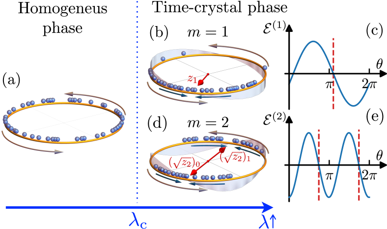
In this work we propose a general mechanism to build custom continuous time crystals in driven diffusive fluids, characterized by an arbitrary number of traveling condensates. Our approach leverages the concept of packing field Hurtado-Gutiérrez et al. (2020), see Fig. 1, a mechanism inspired by the rare event statistics of some driven diffusive systems Bertini et al. (2005); Bodineau and Derrida (2005); Bertini et al. (2006); Derrida ; Hurtado and Garrido (2011); Espigares et al. (2013); Hurtado et al. (2014); Lazarescu (2015); Tizón-Escamilla et al. (2017); Shpielberg et al. (2018); Pérez-Espigares and Hurtado (2019). This packing field pushes particles that lag behind the emergent condensate center of mass while restraining those moving ahead. This amplifies naturally-occurring fluctuations of the particles’ spatial packing, a nonlinear feedback mechanism that eventually leads to a time crystal. From a mathematical perspective, the action of the packing field can be seen as a controlled excitation of the first Fourier mode of the density field fluctuations around the instantaneous center of mass position Hurtado-Gutiérrez et al. (2020), see Fig. 1.(b)-(c). This viewpoint immediately raises the natural question: What happens if we excite higher-order modes? Here we show how this leads to custom and fully controllable continuous time-crystal phases in driven diffusive fluids, characterized by an arbitrary number of rotating condensates, which can be further enhanced with higher-order modes. A local stability analysis of the governing hydrodynamic equations allows us to elucidate the transition to these complex time-crystal phases, as well as general properties of the condensates density profiles and velocities. Using this hydrodynamic picture, we also demonstrate a scaling property of higher-order traveling condensates in terms of first-order ones. These findings are illustrated in several paradigmatic driven diffusive systems, including the random walk fluid Spohn (2012), the Kipnis-Marchioro-Presutti heat transport model Kipnis et al. (1982), the weakly asymmetric simple exclusion process for interacting particle diffusion Spitzer (1970); Derrida (1998), and the Katz-Lebowitz-Spohn lattice gas Katz et al. (1984); Hager et al. (2001); Krapivsky ; Baek et al. (2017). Custom time-crystal phases are demonstrated and characterized in all these models, finding along the way a novel explosive time-crystal phase transition, depending on the nonlinearity of transport coefficients. All together, these results show the versatility and broad possibilities of this promising route to custom time crystals.
The packing-field route to time crystals.— Our starting point is the hydrodynamic evolution equation for the density field in a periodic diffusive system driven by an external field Spohn (2012),
| (1) |
with , and and the diffusivity and the mobility transport coefficients, respectively. The external field takes the form , where is a constant driving that leads to a net current and is the coupling constant to a -th order packing field Hurtado-Gutiérrez et al. (2020). As discussed above, this packing field excites the -th Fourier mode of the density field fluctuations, i.e.
| (2) |
where is the conserved average density. To gain some physical insight on the action of , we define now the complex th-order packing order parameter Hurtado-Gutiérrez et al. (2020); Daido (1992),
| (3) |
Its magnitude measures the packing of the density field around equidistant emergent localization centers placed at angular positions , with . Using , the packing field (2) can be simply rewritten as . In this way, drives particles locally towards the emergent localization centers placed at , pushing particles that lag behind the closest localization center while restraining those moving ahead, with an amplitude proportional to the amount of local packing as measured by , see Figs. 1.b-e. This results in a nonlinear feedback mechanism that amplifies the local packing fluctuations naturally present in the system, resulting eventually in the emergence of traveling-wave condensates for large enough values of , and exhibiting the fingerprints of spontaneous time-translation symmetry breaking.
Hydrodynamic instability and condensate equivalence.— To determine the critical threshold for this instability to happen, we first note that the homogeneous density profile is a solution of Eq. (1). We hence perform a linear stability analysis of this solution and introduce a small perturbation over the flat profile, , with to conserve the global density. Linearizing Eq. (1) and expanding in Fourier modes, it can be shown (see Supp. Mat. SMm ) that the different modes decouple and their stability depend on a competition between the diffusion term and the packing field, controlled by the coupling SMm . This results in the -th Fourier mode of the perturbation becoming unstable when , with
| (4) |
The form of the resulting perturbation beyond the instability SMm is compatible with the emergence of traveling-wave condensates, , moving periodically with an angular velocity right after the instability (), i.e. initially proportional to and . This instability breaks spontaneously the time-translation symmetry of the flat solution, thus giving rise to a continuous time crystal Wilczek (2012); Shapere and Wilczek (2012); Zakrzewski (2012); Richerme (2017); Yao and Nayak (2018); Sacha and Zakrzewski (2018); Sacha (2020); Hurtado-Gutiérrez et al. (2020). Interestingly, the value of increases with , see Eq. (4), a reflection of the competition between diffusion and the packing field. Indeed, while the effect of diffusion, which tends to destroy the emergent condensates, scales as at the instability SMm , the action of the packing field promoting the condensates scales as , and therefore a stronger is needed as increases to destabilize the flat solution. On the other hand, the excess of the averaged current with respect to the homogeneous-phase average current can be shown to be right after the instability SMm , meaning that this current will be larger or smaller than the homogeneous-phase current depending on the mobility curvature for density . This highlights the relevance of transport coefficients in the system’s reaction to the packing field, which enhances or lowers the current and the wave velocity depending on the mobility derivatives.
A remarkable property of the emergent custom time-crystal phase is that the -th-order traveling-wave solution can be built by gluing together copies of the solution after an appropriate rescaling of driving parameters. In particular, it can be shown SMm that , where is the traveling-wave solution of Eq. (1) of velocity for and parameters and , while is the corresponding traveling-wave solution of Eq. (1) of velocity for arbitrary and parameters and . This scaling property, valid for arbitrary nonlinear transport coefficients, allows to collapse traveling-wave solutions for different orders and related driving parameters, reducing the range of possible solutions.
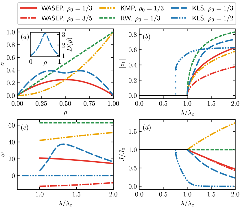
Examples.— To illustrate our findings, we investigate now four paradigmatic driven diffusive models Spohn (2012) under the action of a packing field (2), and which admit a hydrodynamic description of the form of Eq. (1). These models are (i) the random walk (RW) fluid, which captures the diffusive motion of independent particles and is described by a diffusivity and a linear mobility Spohn (2012), (ii) the weakly asymmetric exclusion process (WASEP) that models particle diffusion under exclusion interactions, characterized by and Spitzer (1970); Derrida (1998), (iii) the Kipnis-Marchioro-Presutti (KMP) model of heat transport Kipnis et al. (1982), with and , and (iv) the Katz-Lebowitz-Spohn (KLS) lattice gas model Katz et al. (1984); Hager et al. (2001); Krapivsky ; SMm , which features particle diffusion under on-site exclusion and nearest-neighbors interactions and is described by a nonlinear diffusivity with a sharp maximum and a mobility with a local minimum, see Fig. 2.(a).
All these models, introduced in more detail in the SM SMm , exhibit custom time-crystal phases with novel critical properties. To show this, we solved numerically Eq. (1) using the prescribed and in each case, see SMm . Fig. 2 shows results for , and different values of for each model. In particular, Fig. 2.(b) shows the magnitude of the packing order parameter as a function the coupling . As anticipated above, the homogeneous density profile becomes unstable for , as signaled by the packing of the density field () around an emergent localization center, and a phase transition to a time-crystal phase in the form of a traveling condensate takes place. Interestingly, the transition for the RW, KMP and WASEP models is continuous , see Fig. 2.(b). The velocity of the condensate in these models is initially proportional to and , as predicted, see Fig. 2.(c), and depends monotonously on the coupling . This implies, in particular, a constant positive velocity for the RW model and a positive condensate velocity in the KMP model increasing with . For the WASEP, the sign of changes across due to its particle-hole symmetry: a particle condensate moving to the left for can be seen as a hole condensate moving to the right, and viceversa. The excess current right after the instability depends instead on the value of , see Fig. 2.(d), so that for the KMP ( ) and for the WASEP ( ), while for the non-interacting RW fluid.
Results for the KLS model are more intriguing due to the change of convexity in its mobility and the sharp maximum in the diffusivity, see Fig. 2.(a). In particular, for the KLS lattice gas has and it qualitatively behaves as the WASEP, at least close to the transition. Indeed the transition is continuous, the condensate velocity in positive (), and the excess current is negative (), see blue dashed lines in Figs. 2.(b)-(d), though the KLS condensate velocity is non-monotonous and displays a sharp maximum at a coupling , see Fig. 2.(c). However, the nature of the KLS time-crystal transition changes radically for , where both the order parameter and the excess current present an abrupt, discontinuous change accompanied by a region of bistability and hysteresis for , see Figs. 2.(b),(d), all trademarks of a first-order phase transition. This bistable, first-order-type behavior stems from the pronounced peak in at , see inset to Fig. 2.(a). Indeed, the stability of the condensate depends on the competition between diffusion, washing out any structure, and the packing field (proportional to the packing order parameter), reinforcing the condensate. In the homogeneous phase for we have , so a low density packing competes with almost maximal diffusivity all across the system, difficulting the condensate emergence. On the contrary, if for the same we start from a condensate profile where almost everywhere (except at a sharp region around the condensate walls), we expect a high packing field competing with a low diffusivity, enhancing the condensate stability. This dual behavior explains the first-order scenario observed numerically, and suggests that any model with one or several sharp maxima in diffusivity may exhibit similar phenomenology. Note also that the condensate velocity is zero at due to the particle-hole symmetry of the KLS model Espigares et al. (2013).
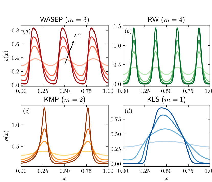
Fig. 3 shows the condensate density profiles obtained numerically for the different models for , varying orders and several supercritical couplings . Interestingly, the shape of the condensate in each case reflects the nonlinear transport properties of the model at hand. For WASEP, the current in the time-crystal phase is lower than in the homogeneous phase due to the exclusion interaction (Fig. 2.(d), ), meaning that the emergence of condensates jams dynamics on average. This jamming gives rise in turn to a sharp density accumulation at the tail of the condensate, see Fig. 3.(a), while the condensate front displays a soft decay as expected due to the available free space. For the KMP heat transport model the picture is complementary: the excess current is positive (), dynamics in the time-crystal phase is faster than in the homogeneous phase, and condensates thus exhibit a sharp front and a softer tail, see Fig. 3.(c). On the other hand, the linearity of the RW fluid implies a completely symmetric condensate shape [Fig. 3.(b)], while the KLS highly nonlinear transport coefficients are reflected in a complex condesate shape, see Fig. 3.(d), with WASEP-like behavior in high- and low- regions where , and KMP-like shape at intermediate densities where . We also note that the driving field controls both the velocity of the resulting condensates and the asymmetry of the associated density profiles (not shown).
Discussion and outlook.— It is interesting to note that the packing field of Eq. (2) can be written as a generalized Kuramoto-like long-range interaction Hurtado-Gutiérrez et al. (2020); Kuramoto and Nishikawa (1987); Pikovsky et al. (2003), while the hydrodynamic equation (1) resembles the one for the oscillator density in the mean-field Kuramoto synchronization model with white noise Acebrón et al. (2005). In this sense, the explosive time-crystal phase transition observed here for the KLS lattice gas resembles similar first-order synchronization transitions in certain oscillator models Leyva et al. (2012); Hu et al. (2014). These links are only formal however, as synchronization models lack any transport in real space, and they are characterized by linear transport coefficients, while the nonlinearity of diffusion and mobility coefficients caused by local exclusion and interactions introduces crucial differences in the observed custom time-crystal phases.
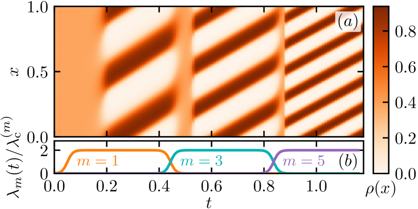
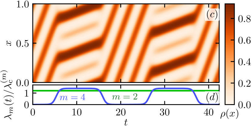
In this work we have shown how to leverage the concept of packing field (2) to engineer custom continuous time crystals in driven diffusive fluids, characterized by multiple rotating condensates. These time-crystal phases can be further enhanced with higher-order matter waves by introducing competing packing fields modulated in time. As a proof of concept, let us consider a generalized external field . Fig. 4 displays the spatiotemporal evolution of the density field that results from the numerical integration of Eq. (1) subject to different generalized external fields. For instance, we may swap between different number of condensates in time as shown in Fig. 4.(a) by switching on and off different orders modulating as in Fig. 4.(b). We may also obtain custom decorated time-crystal phases by switching on and off in time a higher-order mode using as in Fig. 4.(d), in a constant background matter wave obtained by setting . Interestingly, a time-dependent decorated pattern emerges, switching in-phase with between a symmetric time-crystal phase with condensates when and asymmetric condensates when . These simple examples, just two among a myriad of potentially interesting combinations, show the huge potential of the packing-field route to engineer and control custom time-crystal phases in driven diffusive fluids, opening new avenues of future research with promising technological applications. The challenge remains to exploit this route to time crystals in other geometries.
Acknowledgements.
The research leading to these results has received funding from the fellowship FPU17/02191 and from the I+D+i Projects Ref. PID2020-113681GB-I00, Ref. PID2021-128970OA-I00, Ref. C-EXP-251-UGR23 and Ref. P20_00173 financed by the Spanish Ministerio de Ciencia, Innovación y Universidades, Junta de Andalucía-Consejería de Economía y Conocimiento, and the European Regional Development Fund. We are also grateful for the the computing resources and related technical support provided by PROTEUS, the supercomputing center of Institute Carlos I in Granada, Spain.References
- Wilczek (2012) F. Wilczek, “Quantum time crystals,” Phys. Rev. Lett. 109, 160401 (2012).
- Shapere and Wilczek (2012) A. Shapere and F. Wilczek, “Classical time crystals,” Phys. Rev. Lett. 109, 160402 (2012).
- Zakrzewski (2012) J. Zakrzewski, “Crystals of time,” Physics 5, 116 (2012).
- Richerme (2017) P. Richerme, “How to create a time crystal,” Physics 10, 5 (2017).
- Yao and Nayak (2018) N. Y. Yao and C. Nayak, “Time crystals in periodically driven systems,” Physics Today 71, 40 (2018).
- Sacha and Zakrzewski (2018) K. Sacha and J. Zakrzewski, “Time crystals: a review,” Rep. Prog. Phys. 81, 016401 (2018).
- Sacha (2020) Krzysztof Sacha, Time crystals, Vol. 114 (Springer, 2020).
- Bruno (2013) P. Bruno, “Impossibility of spontaneously rotating time crystals: A no-go theorem,” Phys. Rev. Lett. 111, 070402 (2013).
- Nozières (2013) P. Nozières, “Time crystals: Can diamagnetic currents drive a charge density wave into rotation?” Europhys. Lett. 103, 57008 (2013).
- Watanabe and Oshikawa (2015) H. Watanabe and M. Oshikawa, “Absence of quantum time crystals,” Phys. Rev. Lett. 114, 251603 (2015).
- Kozin and Kyriienko (2019) V. K. Kozin and O. Kyriienko, “Quantum time crystals from Hamiltonians with long-range interactions,” Phys. Rev. Lett. 123, 210602 (2019).
- Iemini et al. (2018) F. Iemini et al., “Boundary time crystals,” Phys. Rev. Lett. 121, 035301 (2018).
- Buča et al. (2019) B Buča, J Tindall, and D Jaksch, “Non-stationary coherent quantum many-body dynamics through dissipation,” Nat. Commun. 10, 1730 (2019).
- Keßler et al. (2019) H. Keßler, J. G. Cosme, M. Hemmerling, L. Mathey, and A. Hemmerich, “Emergent limit cycles and time crystal dynamics in an atom-cavity system,” Phys. Rev. A 99, 053605 (2019).
- Carollo et al. (2020) F. Carollo, K. Brandner, and I. Lesanovsky, “Nonequilibrium many-body quantum engine driven by time-translation symmetry breaking,” Phys. Rev. Lett. 125, 240602 (2020).
- Carollo and Lesanovsky (2022) Federico Carollo and Igor Lesanovsky, “Exact solution of a boundary time-crystal phase transition: Time-translation symmetry breaking and non-markovian dynamics of correlations,” Phys. Rev. A 105, L040202 (2022).
- Kongkhambut et al. (2022) P. Kongkhambut et al., “Observation of a continuous time crystal,” Science 377, 670–673 (2022).
- Else et al. (2016) D. V. Else, B. Bauer, and C. Nayak, “Floquet time crystals,” Phys. Rev. Lett. 117, 090402 (2016).
- Moessner and Sondhi (2017) R. Moessner and S. L. Sondhi, “Equilibration and order in quantum Floquet matter,” Nat. Phys. 13, 424 (2017).
- Yao et al. (2017) N. Y. Yao, A. C. Potter, I.-D. Potirniche, and A. Vishwanath, “Discrete time crystals: Rigidity, criticality, and realizations,” Phys. Rev. Lett. 118, 030401 (2017).
- Gong et al. (2018) Z. Gong, R. Hamazaki, and M. Ueda, “Discrete time-crystalline order in cavity and circuit qed systems,” Phys. Rev. Lett. 120, 040404 (2018).
- Gambetta et al. (2019a) F.M. Gambetta, F. Carollo, M. Marcuzzi, J.P. Garrahan, and I. Lesanovsky, “Discrete time crystals in the absence of manifest symmetries or disorder in open quantum systems,” Phys. Rev. Lett. 122, 015701 (2019a).
- Khemani et al. (2019) V. Khemani, R. Moessner, and S..L Sondhi, “A brief history of time crystals,” arXiv:1910.10745 (2019), 10.48550/arXiv.1910.10745.
- Lazarides et al. (2020) A. Lazarides, S. Roy, F. Piazza, and R. Moessner, “Time crystallinity in dissipative floquet systems,” Phys. Rev. Res. 2, 022002 (2020).
- Else et al. (2020) Dominic V. Else, C Monroe, C. Nayak, and N. Y. Yao, “Discrete time crystals,” Annual Review of Condensed Matter Physics 11, 467–499 (2020).
- Zhang et al. (2017) J. Zhang et al., “Observation of a discrete time crystal,” Nature 543, 217 (2017).
- Choi et al. (2017) S. Choi et al., “Observation of discrete time-crystalline order in a disordered dipolar many-body system,” Nature 543, 221 (2017).
- Rovny et al. (2018) J. Rovny, R. L. Blum, and S. E. Barrett, “Observation of discrete-time-crystal signatures in an ordered dipolar many-body system,” Phys. Rev. Lett. 120, 180603 (2018).
- Smits et al. (2018) J. Smits, L. Liao, H. T. C. Stoof, and P. van der Straten, “Observation of a space-time crystal in a superfluid quantum gas,” Phys. Rev. Lett. 121, 185301 (2018).
- Autti et al. (2018) S. Autti, V. B. Eltsov, and G. E. Volovik, “Observation of a time quasicrystal and its transition to a superfluid time crystal,” Phys. Rev. Lett. 120, 215301 (2018).
- O’Sullivan et al. (2020) J. O’Sullivan et al., “Signatures of discrete time crystalline order in dissipative spin ensembles,” New Journal of Physics 22, 085001 (2020).
- Kyprianidis et al. (2021) A. Kyprianidis et al., “Observation of a prethermal discrete time crystal,” Science 372, 1192–1196 (2021).
- Randall et al. (2021) J. Randall et al., “Many-body–localized discrete time crystal with a programmable spin-based quantum simulator,” Science 374, 1474–1478 (2021).
- Xiao et al. (2022) M. Xiao et al., “Time-crystalline eigenstate order on a quantum processor,” Nature 601, 531–536 (2022).
- Keßler et al. (2021) H. Keßler et al., “Observation of a dissipative time crystal,” Phys. Rev. Lett. 127, 043602 (2021).
- Kongkhambut et al. (2021) P. Kongkhambut et al., “Realization of a periodically driven open three-level dicke model,” Phys. Rev. Lett. 127, 253601 (2021).
- Gambetta et al. (2019b) F. M. Gambetta, F. Carollo, A. Lazarides, I. Lesanovsky, and J. P. Garrahan, “Classical stochastic discrete time crystals,” Phys. Rev. E 100, 060105 (2019b).
- Yao et al. (2020) Norman Y. Yao, C. Nayak, L. Balents, and M. P. Zaletel, “Classical discrete time crystals,” Nat. Phys. 16, 438–447 (2020).
- Heugel et al. (2019) T. L. Heugel, M. Oscity, A. Eichler, O. Zilberberg, and R. Chitra, “Classical many-body time crystals,” Phys. Rev. Lett. 123, 124301 (2019).
- Liu et al. (2023) T. Liu, J.-Y. Ou, K. F. MacDonald, and N. I. Zheludev, “Photonic metamaterial analogue of a continuous time crystal,” Nat. Phys. 19, 986–991 (2023).
- Hurtado-Gutiérrez et al. (2020) R. Hurtado-Gutiérrez, F. Carollo, C. Pérez-Espigares, and P. I. Hurtado, “Building continuous time crystals from rare events,” Phys. Rev. Lett. 125, 160601 (2020).
- Bertini et al. (2005) L. Bertini, A. De Sole, D. Gabrielli, G. Jona-Lasinio, and C. Landim, “Current fluctuations in stochastic lattice gases,” Phys. Rev. Lett. 94, 030601 (2005).
- Bodineau and Derrida (2005) T. Bodineau and B. Derrida, “Distribution of current in nonequilibrium diffusive systems and phase transitions,” Phys. Rev. E 72, 066110 (2005).
- Bertini et al. (2006) L. Bertini, A. De Sole, D. Gabrielli, G. Jona-Lasinio, and C. Landim, “Nonequilibrium current fluctuations in stochastic lattice gases,” J. Stat. Phys. 123, 237 (2006).
- (45) B. Derrida, “Non-equilibrium steady states: fluctuations and large deviations of the density and of the current,” J. Stat. Mech. P07023 (2007) .
- Hurtado and Garrido (2011) P. I. Hurtado and P. L. Garrido, “Spontaneous symmetry breaking at the fluctuating level,” Phys. Rev. Lett. 107, 180601 (2011).
- Espigares et al. (2013) C. P. Espigares, P. L. Garrido, and P. I. Hurtado, “Dynamical phase transition for current statistics in a simple driven diffusive system,” Phys. Rev. E 87, 032115 (2013).
- Hurtado et al. (2014) P. I. Hurtado, C. P. Espigares, J. J. del Pozo, and P. L. Garrido, “Thermodynamics of currents in nonequilibrium diffusive systems: theory and simulation,” J. Stat. Phys. 154, 214 (2014).
- Lazarescu (2015) A. Lazarescu, “The physicist’s companion to current fluctuations: one-dimensional bulk-driven lattice gases,” J. Phys. A 48, 503001 (2015).
- Tizón-Escamilla et al. (2017) N. Tizón-Escamilla, C. Pérez-Espigares, P. L. Garrido, and P. I. Hurtado, “Order and symmetry-breaking in the fluctuations of driven systems,” Phys. Rev. Lett. 119, 090602 (2017).
- Shpielberg et al. (2018) O. Shpielberg, T. Nemoto, and J. Caetano, “Universality in dynamical phase transitions of diffusive systems,” Phys. Rev. E 98, 052116 (2018).
- Pérez-Espigares and Hurtado (2019) C. Pérez-Espigares and P. I. Hurtado, “Sampling rare events across dynamical phase transitions,” Chaos 29, 083106 (2019).
- Spohn (2012) H. Spohn, Large Scale Dynamics of Interacting Particles, Theoretical and Mathematical Physics (Springer Berlin Heidelberg, 2012).
- Kipnis et al. (1982) C. Kipnis, C. Marchioro, and E. Presutti, “Heat-flow in an exactly solvable model,” J. Stat. Phys. 27, 65 (1982).
- Spitzer (1970) F. Spitzer, “Interaction of markov processes,” Adv. Math. 5, 246 (1970).
- Derrida (1998) B. Derrida, “An exactly soluble non-equilibrium system: The asymmetric simple exclusion process,” Phys. Rep. 301, 65 (1998).
- Katz et al. (1984) S. Katz, J. L. Lebowitz, and H. Spohn, “Nonequilibrium steady states of stochastic lattice gas models of fast ionic conductors,” J. Stat. Phys. 34, 497–537 (1984).
- Hager et al. (2001) J. S. Hager, J. Krug, V. Popkov, and G. M. Schütz, “Minimal current phase and universal boundary layers in driven diffusive systems,” Phys. Rev. E 63, 056110 (2001).
- (59) P. L. Krapivsky, “Dynamics of repulsion processes,” J. Stat. Mech. P06012 (2013) , P06012.
- Baek et al. (2017) Y. Baek, Y. Kafri, and V. Lecomte, “Dynamical symmetry breaking and phase transitions in driven diffusive systems,” Phys. Rev. Lett. 118, 030604 (2017).
- Daido (1992) Hiroaki Daido, “Order function and macroscopic mutual entrainment in uniformly coupled limit-cycle oscillators,” Prog. Theor. Phys. 88, 1213–1218 (1992).
- (62) See the Supplemental Material for a detailed derivation of the critical value of the amplitude and the equivalence of the condensates.
- Kuramoto and Nishikawa (1987) Y. Kuramoto and I. Nishikawa, “Statistical macrodynamics of large dynamical systems. Case of a phase transition in oscillator communities,” J. Stat. Phys. 49, 569 (1987).
- Pikovsky et al. (2003) A. Pikovsky, M. Rosenblum, and J. Kurths, Synchronization: A Universal Concept in Nonlinear Sciences (Cambridge University Press, Cambridge, 2003).
- Acebrón et al. (2005) J. A. Acebrón, L. L. Bonilla, C. J. Pérez Vicente, F. Ritort, and R. Spigler, “The Kuramoto model: A simple paradigm for synchronization phenomena,” Rev. Mod. Phys. 77, 137 (2005).
- Leyva et al. (2012) I. Leyva et al., “Explosive first-order transition to synchrony in networked chaotic oscillators,” Phys. Rev. Lett. 108, 168702 (2012).
- Hu et al. (2014) X. Hu et al., “Exact solution for first-order synchronization transition in a generalized kuramoto model,” Scientific Reports 4, 7262 (2014).
- Delabays (2019) Robin Delabays, “Dynamical equivalence between kuramoto models with first- and higher-order coupling,” Chaos: An Interdisciplinary Journal of Nonlinear Science 29, 113129 (2019).
- Hurtado and Garrido (2009) P. I. Hurtado and P. L. Garrido, “Test of the additivity principle for current fluctuations in a model of heat conduction,” Phys. Rev. Lett. 102, 250601 (2009).
- Baek and Kafri (2015) Y. Baek and Y. Kafri, “Singularities in large deviation functions,” J. Stat. Mech. 2015, P08026 (2015).
- Press et al. (2007) William H Press, Saul A Teukolsky, William T Vetterling, and Brian P Flannery, Numerical recipes 3rd edition, 3rd ed. (Cambridge University Press, Cambridge, England, 2007).
SUPPLEMENTAL MATERIAL
Exploiting the packing-field route to craft custom time crystals
R. Hurtado-Gutiérrez1,2, C. Pérez-Espigares1,2, P.I. Hurtado1,2,
1Departamento de Electromagnetismo y Física de la Materia,
Universidad de Granada, 18071 Granada, Spain
2Institute Carlos I for Theoretical and Computational Physics,
Universidad de Granada, 18071 Granada, Spain
S1 I. Hydrodynamic instability in the time-crystal phase transition
Our starting point is the hydrodynamic evolution equation for the density field in a periodic diffusive system driven by an external field ,
| (S1) |
with , and and the diffusivity and the mobility transport coefficients, respectively. The external field takes the form , where is a constant driving and is the coupling to a -th order packing field , defined as
| (S2) |
where is the conserved average density. To better understand the action of , we define now the complex th-order packing order parameter (also known as the Kuramoto-Daido order parameter in the context of synchronization transitions),
| (S3) |
Its magnitude measures the packing of the density field around equidistant emergent localization centers placed at angular positions , with . Using , the packing field of Eq. (S2) can be simply rewritten as . In this way, drives particles locally towards the emergent localization centers placed at , pushing particles that lag behind the closest localization center while restraining those moving ahead, with an amplitude proportional to the amount of local packing as measured by . This results in a nonlinear feedback mechanism that amplifies the local packing fluctuations naturally present in the system, resulting eventually in the emergence of traveling-wave condensates for large enough values of , and exhibiting the fingerprints of spontaneous time-translation symmetry breaking.
To determine the critical threshold for this instability to happen, we first note that for any value of the homogeneous density profile is a solution of the hydrodynamic equation (S1). Therefore, a linear stability analysis of this solution will allow us to find the critical value . We hence consider a small perturbation over the flat profile, , with so as to conserve the global density of the system. Plugging this perturbation into Eq. (S1) and linearizing it to first order in we obtain
| (S4) |
where stands for the derivative of the mobility with respect to its argument evaluated at , and where we have used that is already first-order in , see Eq. (S3). The system periodicity can be used to expand the density field perturbation in Fourier modes,
| (S5) |
where the -th Fourier coefficient is given by . Noting that the Kuramoto-Daido parameter is proportional to the -th Fourier coefficient in this expansion, i.e. , and replacing the Fourier expansion in Eq. (S4), we obtain
| (S6) |
where we have defined
| (S7) |
and and are Kronecker deltas. As the different complex exponentials in Eq. (S6) are linearly independent, each parenthesis in the equation must be zero. Therefore the solution for the different Fourier coefficients is just
| (S8) |
with the coefficients associated with the initial perturbation . The stability of the different Fourier modes is then controlled by the real part of , for which we have to consider two distinct cases: and . In the first case , we have , so that these Fourier modes will always decay. On the other hand, when , the decay rate involves a competition between the diffusion term and the packing field,
| (S9) |
The critical value of is reached whenever , and reads
| (S10) |
In this way we expect the homogeneous density solution to become unstable for , leading to a density field solution with a more complex spatiotemporal structure.
The previous analysis shows that, right after the instability, the first modes to become unstable and contribute to a structured density field will be the -order Fourier modes. In this regime we therefore expect a traveling-wave solution with a small amplitude and where the angular velocity is given from the imaginary part of Eq. (S7),
| (S11) |
This suggests that beyond the instability, the homogeneous density turns into condensates periodically moving at a constant velocity (initially proportional to and ), thus giving rise to a custom continuous time crystal. Moreover, the average current associated to this traveling-wave solution right after the instability can be calculated from the local current in the linearized equation (S4), resulting in
| (S12) |
where is the average current in the homogeneous phase. While we only expect Eqs. (S11)-(S12) to hold true close to , they highlight the relevance of the transport coefficients in the response of the model to the packing field. Depending on the slope and convexity of the mobility of each model, the packing field will enhance or lower the current and the speed of the resulting condensates.
S2 II. Mapping condensate profiles across different packing orders
In this section we investigate the relation between traveling-wave solutions to Eq. (S1) corresponding to different packing orders . In particular we will show that, provided that a -periodic traveling-wave solution of Eq. (S1) exists for packing order , this solution can be built by gluing together copies of the solution of the equation with properly rescaled parameters. To prove this, we start by using a traveling-wave ansatz in the hydrodynamic equation (S1) with packing order , where is a generic periodic function and denotes the traveling-wave velocity. This leads to
| (S13) |
where we have introduced the variable . In addition, we have used that under the traveling-wave ansatz the magnitude of the order parameter is constant and its complex phase increases linearly in time, i.e., with .
Since we expect the formation of equivalent particle condensates once the homogeneous density profile becomes unstable, it seems reasonable to assume that the resulting traveling density wave will exhibit -periodic behavior, i.e. with a new -periodic function. Under this additional assumption, the initial -th order Kuramoto-Daido parameter reads
| (S14) |
where we haven taken into account the periodicity of and where is defined as the initial Kuramoto-Daido parameter of . Using this result we can rewrite Eq. (S13) in terms of and a new variable ,
| (S15) |
where we have used that . This is nothing but the original equation for the traveling wave Eq. (S13) with a packing order and rescaled parameters
| (S16) |
In this way, we have proved that if is a traveling-wave solution of the hydrodynamic equation (S1) with and parameters and , then is a solution of the corresponding hydrodynamic equation with order and parameters and . Note that this result resembles the one found in the Kuramoto model, where a complete dynamical equivalence between the first-order and higher-order couplings has been reported Delabays (2019).
S3 III. Driven diffusive models
The general results obtained in this paper have been illustrated by solving the hydrodynamic equations for several paradigmatic driven diffusive systems, including the random walk (RW) fluid Spohn (2012), the weakly asymmetric simple exclusion process (WASEP) for interacting particle diffusion Spitzer (1970); Derrida (1998), the Kipnis-Marchioro-Presutti (KMP) heat transport model Kipnis et al. (1982), and the Katz-Lebowitz-Spohn (KLS) lattice gas Katz et al. (1984); Hager et al. (2001); Krapivsky . In this appendix we briefly introduce these microscopic lattice models and their hydrodynamic description. We define the microscopic models on a lattice of size with periodic boundary conditions, though they can be easily generalized to arbitrary dimension and different boundary conditions. As for their hydrodynamic description, it takes in all cases a standard diffusive form for a mesoscopic density field ,
| (S17) |
with , and the diffusivity and the mobility transport coefficients, respectively, and some external field that drives the system to a nonequilibrium steady state of global density and a net current .
The RW fluid is composed by independent particles which jump stochastically and sequentially to nearest neighbor lattice sites with rates for jumps along the -direction, with the lattice size such that . At the hydrodynamic level, the RW fluid is characterized by a diffusivity and a mobility Spohn (2012). This linear dependence of the mobility on the density field is a signature of the noninteracting character of the RW fluid.
The weakly asymmetric simple exclusion process (WASEP) Spitzer (1970); Derrida (1998) is a stochastic particle system similar to the RW fluid, but with the crucial addition of a exclusion interactions. In particular, in the WASEP particles live in a periodic lattice of size , such that each lattice site may contain at most one particle. Dynamics is stochastic and proceeds via sequential particle jumps to nearest-neighbor sites, provided these are empty (in other case the exclusion interaction forbides the jump), at a rate for jumps along the -direction. At the macroscopic level the WASEP is characterized by a diffusivity and a mobility , a quadratic dependence on the local density clearly reflecting the key role of the exclusion interaction.
In the Kipnis-Marchioro-Presutti (KMP) model of heat transport Kipnis et al. (1982); Hurtado and Garrido (2009, 2011), each lattice site is characterized by a non-negative amount of energy . Dynamics is stochastic, proceeding through random energy exchanges between randomly chosen nearest neighbors , in such a way that the total pair energy is conserved in the collision. At the hydrodynamic level, the KMP model is characterized by a diffusivity and a mobility .
The Katz-Lebowitz-Spohn (KLS) lattice gas model is a stochastic particle systems that features on-site exclusion and nearest-neighbor interactions Katz et al. (1984); Hager et al. (2001); Krapivsky ; Baek and Kafri (2015). In the KLS model each lattice site can be empty or occupied by one particle at most. The model is defined by two parameters, and , which control the particle hopping dynamics with rates , , , and . Note that spatially inverted versions of these transitions occur with identical rates Baek and Kafri (2015). In contrast to the other microscopic transport models presented above, the richer dynamics of the KLS model leads to more complex transport coefficients at the macroscopic level. Specifically, the diffusion coefficient is obtained in terms of the quotient
| (S18) |
where is the average current in the totally asymmetric version of the model and is its compressibility. The first is given by
| (S19) |
while the second obeys,
| (S20) |
Parameters and are determined in turn from the expressions
| (S21) |
Finally the mobility coefficient is obtained from the diffusion coefficient and the compressibility using the Einstein relation . For this paper we have chosen to work with parameters and , which results in a nonlinear diffusivity with a sharp maximum and a mobility with a local minimum, see Fig. 2.(a) in the main text.
S4 IV. Solving numerically the traveling-wave hydrodynamical equation
In this appendix, we detail the numerical method used in this work to calculate the traveling-wave solutions to Eq. (S1), i.e.
| (S22) |
with , periodic boundary conditions, and the Kuramoto-Daido parameter given by
| (S23) |
This is a nonlinear second-order integro-differential equation that poses a challenge for standard numerical methods. In particular, reaching the traveling-wave regime with enough precision using standard techniques for partial differential equations—such as finite difference methods— becomes increasingly difficult when the system is either close to the critical point or deep into the nonlinear regime.
To address this problem, we have devised an alternative approach based on transforming this equation into an ordinary first-order differential equation supplemented by several self-consistence relations. For that, we consider the hydrodynamic equation (S22) with a traveling-wave ansatz to obtain an ordinary second-order differential equation in terms of the variable ,
| (S24) |
Here we have used that, under the traveling wave ansatz, the magnitude of the order parameter is constant and its complex phase increases linearly in time, i.e., with the complex argument at . This simplifies the equation on one hand, but it makes it harder to deal with the order parameter. In the original partial differential equation, given the density profile at a particular time step, we just needed to evaluate in order to obtain the next one. However, in the traveling-wave version of Eq. (S24), in order to compute the differential equation we need the integral Eq. (S23) of its solution, which renders usual differential equations methods invalid.
To overcome this issue, we first integrate Eq. (S24) to obtain a first-order differential equation easier to tackle numerically,
| (S25) |
where is an integration constant and we have chosen without loss of generality (i.e. we set the origin of to the angular position given by , so ). The key step now is to consider as a free parameter instead of the integral of the solution, thus transforming the previous equation into a standard ordinary differential equation depending on three parameters: , , and . Such a differential equation can now be solved using the initial condition at the left boundary to obtain the solution . Nevertheless, this function is not in general a solution to the original problem. The parameters , , , and must be carefully chosen to ensure the compatibility of the solution with the specifications of the original problem: the periodicity of the solution, its average density and the consistency between the chosen and the value calculated from . These conditions are captured in the following system of equations,
| (periodicity) | (S26) | |||
| (average density) | (S27) | |||
| (S29) |
which complete the set of equations required to solve the problem (we have two real equations and a complex one to determine four real parameters). To determine the solution to the original problem, we define a function which calculates the profile using Eq. (S25) and returns the squared sum of the errors in the previous self-consistent equations for this profile. With this, the correct parameters can be found by performing a numerical optimization of , and the traveling wave profile corresponding to such parameters will be the solution of the original problem. This approach is reminiscent of the shooting method Press et al. (2007) used to solve two-point boundary value problems.