Refined cyclic renormalization group in Russian Doll model
Abstract
We discuss the Russian Doll Model (RDM) of superconductivity for finite energy levels. Previously, cyclic renormalization group (RG) and Efimov scaling were found in RDM for part of the equidistant spectrum and we generalize this observation in a few directions. We find that when the whole spectrum is considered, equidistancy condition is removed or diagonal disorder is added, the cyclicity of RG survives but the period of RG becomes energy dependent. The analytic analysis is supported with exact diagonalization.
1 Introduction
The Richardson model of superconductivity [28, 29] is a suitable toy model with finite number of degrees of freedom which allows to capture the key properties of superconducting state in a relatively simple manner. The model is integrable and the corresponding spectrum can be obtained via the Bethe Ansatz (BA) equations which coincide with the BA equations for the twisted SU(2) Gaudin model [10]. The commuting Hamiltonians of the Richardson model get identified as superpositions of the Gaudin Hamiltonians.
There is a simple integrable deformation of the Richardson model – the so-called Russian Doll model (RDM) [19, 20] which involves the time-reversal (T) symmetry breaking deformation parameter. In this case, the BA equations for the spectrum are identical to the BA equations for the twisted inhomogeneous XXX spin chain. The inhomogeneities get identified with the energy levels of RDM model while the twist is the counterpart of the coupling constant in RDM. The T-symmetry breaking parameter in RDM is identified as the "Planck constant" in XXX spin chain which vanishes in the Gaudin limit [11]. The model can also be related to Chern-Simons theory when the excitations are represented by vertex operators [3].
The RDM model exhibits a rare property — it hosts cyclic renormalization group (RG) flows for the couplings [19]. The RG parameter is where N is number of energy levels and the step in RG is "integrating out" the highest energy level. The coupling evolves in a cyclic manner while the T-symmetry breaking parameter fixes the period of the cycle. The RG cycle implies a nontrivial interplay between the ultraviolet- (UV) and infrared-limit (IR) physics, and the underlying algebraic property was identified as the anomalous breaking of scale invariance down to the discrete subgroup [2, 23].
Due to the remaining discrete scale invariance in the models with cyclic RG flows some part of the spectrum obeys the so-called Efimov exponential scaling . In the RDM, Efimov scaling has been found for the hierarchy of gaps, see [9] for a review. Note that recently new examples of cyclic RG [15], as well as examples of homoclinic RG orbits [14] and chaotic RG flows [7] have been found.
The ensemble averaging of the Richardson model with some measure for the diagonal on-site disorder has been considered in [27, 21, 26, 25, 18]. The measure for the ensemble averaging is a bit arbitrary and the relevance of the Generalized Gibbs Ensemble (GGE) for the disordered Richardson model has been discussed. The corresponding level statistics has been identified.
The effective Hamiltonian provides the possibility to elaborate the localization properties of the one-particle states. Of particular interest is whether our model shows the non-ergodic, but extended phase (usually called fractal or multifractal) for some values of of the coupling strength . Recall that fractal behavior has been observed in several models [17, 12, 31, 22, 32, 6, 26, 25, 18, 30, 4, 24, 8] and the Rosenzweig-Porter model (RPM) is the most familiar example, where multifractality has been found for the interval [17]. Later the fractal behavior of RPM was confirmed within other approaches [12, 31, 6, 22, 32]. Using effective momentum-space RG and Fermi’s Golden Rule, we have found that one-particle states in our version of RDM demonstrates a fractality interval as well [24]. The fractal dimension is determined exactly and equals .
In this study, we shall generalize the cyclic RG for couplings developed in [19] for the case of equidistant spectrum. First, we make a refinement of the cyclic RG for all energies for equidistant as well as non-equidistant spectra and find that the cyclic RG structure survives but the period of the RG becomes energy-dependent. The next aim is the derivation of the RG for the random RDM with diagonal disorder. The analysis yields a similar result – the period of the RG becomes energy- and disorder-dependent. We also comment on the fate of the Efimov tower and the incomplete breaking of scale invariance in these cases.
Note that the T-breaking parameter is usually not renormalized perturbatively, but can be renormalized however if some kind of non-perturbative effects are taken into account. An example of RG in a disordered system with Anderson localization and T-breaking can be found in [1].
2 Model
We consider the random matrix model of the following form
| (1) |
Note that we consider open boundary conditions and put the overall energy shift to zero without loss of generality. Here is a certain (might be random and non-monotonic) potential of on a finite support
| (2) |
3 Sierra’s Renormalization group (RG) for all energies.
3.1 RG for equidistant spectrum
In Ref. [19] the authors consider the model (1) in the bosonic setting for application to superconductivity, with the following choice for the parameter
| (3) |
with being the bandwidth 111Unlike [19], we use for the total bandwidth, not its half and for the level spacing, not its half. of the diagonal potential. They focused on the case with equidistant spectrum of the diagonal potential
| (4) |
with a certain energy shift (if not mentioned otherwise, we will use ), giving the range of the diagonal energies as in (2). They derived the following renormalization group (RG), see Eq. (15) in Ref. [19], removing the largest diagonal energy level at each step:
| (5) |
In order to derive the above equations the authors of [19] did the following:
-
1.
First, they start with the matrix of size and at each step reduce its size by one.
-
2.
For this, they take at each step the level with the largest diagonal energy in the absolute value ( or ).
-
3.
Assuming it to be large with respect to the rest of the levels, they resolve the eigenproblem with respect to it (say ):
(6a) (6b) Strictly speaking, the latter fraction was split into two terms with replaced by and , respectively, but this was not important for them.
-
4.
Next, they assumed and using the ratio they end up with Eqs. (5).
The solution of Eqs. (5) can be found in the continuous limit ds
| (7a) | ||||
| (7b) | ||||
with and . Strictly speaking the above RG works for the bottom of the spectrum if one takes the energies always from the top of the spectrum.
3.2 Energy dependent RG periods
In general, one should replace the assumption in item 4 by the correct expression
| (8) |
Now the renormalization variable should be defined as
| (9) |
where and one arrives at the same RG equations and solution as Eqs.(15-16) in [19]
| (10) |
The validity of the above equation (10) is limited by the conditions for the absence of resonance
| (11) |
The first condition ensures that the increment in the integral (9) is small, while the second one limits the increment in (10) to make the derivation from (8) to it valid. Note that from Eq. (9) one can see that the monotonicity of the parameter (9) depends on the energy and does not necessarily require the monotonicity of . Indeed, for , even random does not change the monotonic behavior of . In the following two subsections, we apply the above considerations for equidistant and disordered diagonal potentials.
3.3 Entire spectrum for equidistant potential
For equidistant diagonal potential (4), one can introduce the following parameter , for the energy shift, which gives:
| (12) |
As in Eq.(17) of [19] the result (10) is periodic with the period in . The period in corresponds to the change in the matrix size given by
| (13) |
The number of periods before goes as
| (14) |
However, unlike [19], here we see two peculiarities:
-
•
First, the period in is energy -dependent, Eq. (13), and
-
•
Second, there is the singularity at , or equivalently, at .
The latter is important for the understanding of the following fact. Indeed, according to [19] and Eq. (13), the matrix size shrinks by and the spectrum repeats itself with the shift by one level. However, on the way from to other levels have also disappeared. Where have they gone?
To answer this physical question, one should consider the continuity condition (11) more closely. What happens when this condition is violated? In such a case, one cannot transform the sum in Eq. (9) to the integral and, moreover, already at one step one of the increments or is not small. This means that many periods can pass in this region without being seen in numerics. Strictly speaking, each RG step (8) corresponds to the removal of one column and one row of the matrix and can be considered as a rank- perturbation for the matrix [5]. As it is known from Richardson’s model [21] and other works [18, 16], such a rank- perturbation can move significantly only one (top or bottom) level , while the other levels are bound in between the ones at the previous step
| (15) |
This means that independently of the condition (11) only one level disappears from the spectrum by going to the drain at in the RG step. We will show the same in our numerical results in Sec. 4.
3.4 Case of the diagonal disorder
Strictly speaking Eqs. (8) and (9) work for any diagonal potential, not only for equidistant or monotonic . Therefore in this subsection we consider disordered diagonal potential. In the case when the diagonal energies are not equidistant (4) but given by independent random numbers, the derivation of RG equations from (6) is not completely trivial.
In order to make the derivation clear let’s consider separately the two effects of the disorder:
-
1.
Fluctuations of around their mean value (4);
-
2.
Re-shuffling of .
Taking into account only the first effect, one can represent as a sum of independent increments
| (16) |
For large enough , Eq. (4), of i.i.d. random elements in the sum , can be approximated by a Gaussian random number with the following mean and variance
| (17) |
and thus can be represented as
| (18) |
with the standard Gaussian variable
| (19) |
The corresponding increment , Eq. (9), is then given by
| (20) |
With the latter Taylor expansion this gives the result for in terms of the central limit theorem as
| (21) |
Here we used the central limit theorem for the sum of Gaussians with zero means and variances and introduced another standard Gaussian variable , Eq. (19).
From the latter one can see that the additional summand to with respect to the one in the disorder-free case, Eq. (12), is small compared to the period for large enough within the RG validity region, Eq. (11). Strictly speaking, in the sum (21) one cannot keep the terms as the Euler-Mascheroni constant is also neglected there.
At the same time, at the top of the spectrum (from where we take out ) and close to the fluctuations will be important already at the level of Eq. (20). In the former region the central limit theorem in (18) does not hold, while in the latter the entire validity of the RG (11) is broken. As a result, the periodicity of the spectrum partly survives in the monotonic but disordered diagonal potential.
The reshuffling of the diagonal disorder has another effect. Indeed, as we mentioned in Sec. 3.2, in this case the monotonicity of the periodicity parameter is guaranteed only for . Therefore, the above periodicity (10) survives only in that region, while within the diagonal band, , the parameter can be non-monotonic with and random, and therefore no periodicity is expected.
3.5 Generalized Efimov scaling
Let us comment on the place of our study in the general context of the two-parametric RG flows when one parameter induces T-symmetry breaking. It is useful to introduce the following modular parameter [13]
| (22) |
The real part is the chemical potential for the topological number of any nature, say, winding, topological charge etc. On the other hand the imaginary part is any parameter quantifying disorder, say, coupling constant, diffusion coefficient, boundary condition etc. In our case one could have in mind while, for example , for the Anderson model in 1d with T-symmetry breaking term and the diffusion coefficient [1]. Before renormalization there is the natural action of on modular domain of .
The pattern of RG orbits considered as trajectories of the dynamical systems depends on the relative weights of the perturbative and non-perturbative contributions to the -functions. The conventional cyclic RG occurs at stable fixed point for taking into account only a first perturbative contribution to the . The is finite at the stable fixed point and it governs the period of the RG cycle (10). Generically both the ’s are elliptic functions of the modular parameter and behave differently in the limiting cases.
The RG flow towards the stable fixed point can occur through the chain of unstable fixed points for . For instance, such behavior and interesting universality has been observed in [13] in the limit when the potential function for the RG flow which yields the function is the generalized Dedekind function.
| (23) |
where is Dedekind function . At small fixed the RG potential for T-breaking parameter gets reduced to whose minima exhibit the interesting recurrence for the unstable critical points of the RG flow for . The recurrence is ruled by the free group which is subgroup of and involves three generators of the discrete RG flows [13]. At the RG flows to the stable critical point while a topological parameter tends to the Golden ratio . This model example corresponds to the one-dimensional Penrose model which is a toy model exhibiting cyclic RG cycle. In that case the Efimov scaling for the bound states reads as
| (24) |
with . In the refined RG, once again we look at the stable fixed point of but the period of is energy dependent
| (25) |
A bit loosely we could say that the defining the period at the fixed point is E-dependent. Instead of (24) we have scaling of the form
| (26) |
which reduces to Efimov scaling for equidistant spectrum. Note that the Efimov scaling follows from the partial breaking of the scale invariance down to the discrete subgroup [2, 23]. In the refined case the discrete subgroup is broken as well.
4 Numerics
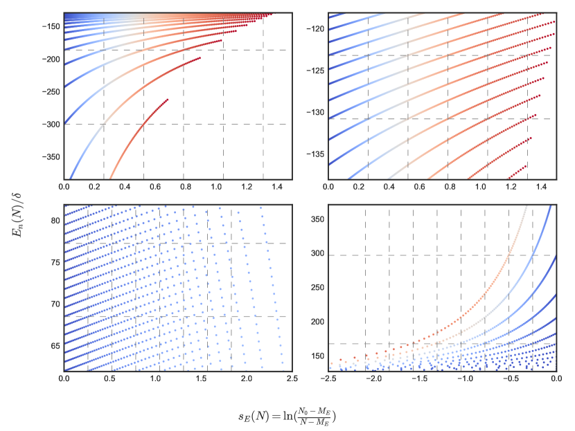
In order to check the analytical predictions of the previous section, we have performed numerical simulations similar to [19]. Taking the initial Hamiltonian (1) of size , we compute the spectrum for the models, given by the first rows and columns of the matrix. Then the spectrum of such models (normalized by the parameter ) has been plotted versus the periodicity parameter , Eq. (9), see Figs. 1 – 3. For our numerics we have chosen , , and , though the results are qualitatively the same for other parameters as well.
In the case of the equidistant spectrum, Fig. 1, the periodicity parameter is given by (12), , with . One can see from Fig. 1 that the periodicity differs in different regions of the spectrum, but it is still given by the above formula. At the spectral edges (see the first and last panels), the energy levels may disappear with decreasing (and increasing ). In addition, close to the energies , (see the bottom part of the last panel in Fig. 1), the periodicity is violated in full agreement with the validity range, Eq. (11). Note that it is not just the discreteness of the spectrum which matters as for smaller energies even the discrete spectrum shows the same periodicity, cf. left () and right () bottom panels.
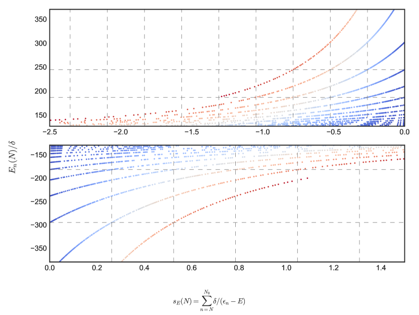
In the more physical and interesting case of disordered diagonal potential (17), one has to modify the periodicity parameter to (9) or in the monotonic case to (21). In this case, see Fig. 2, the periodicity is still clearly seen, but close to the interval of the diagonal potential energies, (with ) the periodic levels are not seen under the ones with random shifts along . The latter are those levels, which hit the resonance and, thus, have non-monotonic vs .
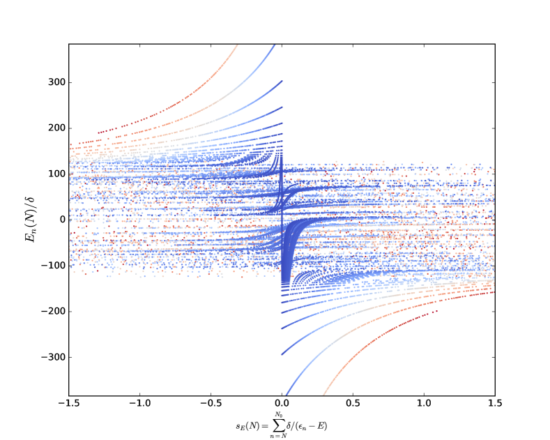
In order to show clearly the range of random energies, we plot the entire spectrum of the system in Fig. 3 versus the local periodicity parameter . From that figure the periodicity is hard to see due to the symbol sizes, but one can clearly observe that in the interval the random levels, corresponding to the above hitting of resonances and non-monotonic , prevails over the the regular ones, so the latter are not seen. Beyond the above mentioned energy interval, i.e. for , no such random levels are visible.
In addition, a random singular point of the spectrum appears at , where the regular spectral part changes behavior from at to otherwise. These are exactly the sink points which are random within the interval at each step where most of the levels disappear beyond RG periodicity.
5 Conclusion
In this paper we have generalized the periodic renormalization group (RG) for the known Russian Doll model (RDM) in several ways.
In the original RDM with the equidistant diagonal elements, we have shown that the RG period depends significantly on the energy interval and has a singularity at the sink point . It is this singularity which compensates the disbalance of energy levels that should disappear after the RG period and, according to the previous literature [19, 20], shift the entire spectrum by one level only.
In addition, we have considered the RDM with the disordered diagonal elements and found a generalized RG parameter over which RG equations are still periodic, at least in the spectral parts lying beyond the energy interval of the diagonal elements. We have considered both the effects of small oscillations of the diagonal elements as well as their re-shuffling due to disorder.
All the analytical predictions have been confirmed by the numerical simulations. It would be interesting to identify the limit cycle breaking discussed in this study with the generic framework of breakdown of the limit cycle in the bifurcation theory.
6 Acknowledgments
V. M. thanks MPIPKS for providing an opportunity to take part in the Summer Internship program during which this project was initiated and acknowledges support from the Harding Foundation. I. M. K. acknowledges support by the Russian Science Foundation (Grant No. 21-72-10161). A. S. G. thanks Nordita and IHES where the parts of this work have been done for the hospitality and support.
References
- Altland et al. [2015] Alexander Altland, Dmitry Bagrets, and Alex Kamenev. Topology versus Anderson localization: Nonperturbative solutions in one dimension. Phys. Rev. B, 91:085429, Feb 2015. doi: 10.1103/PhysRevB.91.085429. URL https://link.aps.org/doi/10.1103/PhysRevB.91.085429.
- Ananos et al. [2003] Gino NJ Ananos, Horacio E Camblong, Carlos Gorrichátegui, Ernesto Hernández, and Carlos R Ordonez. Anomalous commutator algebra for conformal quantum mechanics. Physical Review D, 67(4):045018, 2003.
- Asorey et al. [2002] Manuel Asorey, Fernando Falceto, and Germán Sierra. Chern-Simons theory and BCS superconductivity. Nucl. Phys. B, 622(3):593–614, 2002. ISSN 0550-3213. doi: 10.1016/S0550-3213(01)00614-9. URL https://www.sciencedirect.com/science/article/pii/S0550321301006149.
- Biroli and Tarzia [2021] G. Biroli and M. Tarzia. Lévy-Rosenzweig-Porter random matrix ensemble. Phys. Rev. B, 103:104205, Mar 2021. doi: 10.1103/PhysRevB.103.104205. URL https://link.aps.org/doi/10.1103/PhysRevB.103.104205.
- Bogomolny [2017] E. Bogomolny. Modification of the porter-thomas distribution by rank-one interaction. Phys. Rev. Lett., 118:022501, Jan 2017. doi: 10.1103/PhysRevLett.118.022501. URL https://link.aps.org/doi/10.1103/PhysRevLett.118.022501.
- Bogomolny and Sieber [2018] E. Bogomolny and M. Sieber. Eigenfunction distribution for the Rosenzweig-Porter model. Phys. Rev. E, 98:032139, Sep 2018. doi: 10.1103/PhysRevE.98.032139. URL https://link.aps.org/doi/10.1103/PhysRevE.98.032139.
- Bosschaert et al. [2022] Maikel M Bosschaert, Christian B Jepsen, and Fedor K Popov. Chaotic rg flow in tensor models. Physical Review D, 105(6):065021, 2022.
- Buijsman and Lev [2022] Wouter Buijsman and Yevgeny Bar Lev. Circular Rosenzweig-Porter random matrix ensemble. SciPost Phys., 12:82, 2022. doi: 10.21468/SciPostPhys.12.3.082. URL https://scipost.org/10.21468/SciPostPhys.12.3.082.
- Bulycheva and Gorskii [2014] K. M. Bulycheva and A. S. Gorskii. Limit cycles in renormalization group dynamics. Phys. Usp., 57(2):171–182, 2014. doi: 10.3367/UFNe.0184.201402g.0182. URL https://ufn.ru/en/articles/2014/2/g/.
- Cambiaggio et al. [1997] M. C. Cambiaggio, A. M. F. Rivas, and M. Saraceno. Integrability of the pairing hamiltonian. Nuclear Physics A, 624(2):157–167, 1997. ISSN 0375-9474. doi: 10.1016/S0375-9474(97)00418-1. URL https://www.sciencedirect.com/science/article/pii/S0375947497004181.
- Dunning and Links [2004] C. Dunning and J. Links. Integrability of the Russian doll BCS model. Nucl. Phys. B, 702(3):481–494, 2004. ISSN 0550-3213. doi: 10.1016/j.nuclphysb.2004.09.021. URL https://www.sciencedirect.com/science/article/pii/S0550321304007278.
- Facoetti et al. [2016] D. Facoetti, P. Vivo, and G. Biroli. From non-ergodic eigenvectors to local resolvent statistics and back: A random matrix perspective. Europhys. Lett., 115:47003, 2016. doi: 10.1209/0295-5075/115/47003. URL https://doi.org/10.1209%2F0295-5075%2F115%2F47003.
- Flack et al. [2023] Ana Flack, Alexander Gorsky, and Sergei Nechaev. Generalized devil’s staircase and rg flows. Nuclear Physics B, 996:116376, 2023.
- Jepsen and Popov [2021] Christian B Jepsen and Fedor K Popov. Homoclinic renormalization group flows, or when relevant operators become irrelevant. Physical Review Letters, 127(14):141602, 2021.
- Jepsen et al. [2021] Christian B Jepsen, Igor R Klebanov, and Fedor K Popov. Rg limit cycles and unconventional fixed points in perturbative qft. Physical Review D, 103(4):046015, 2021.
- Kochergin et al. [2024] Daniil Kochergin, Ivan M. Khaymovich, Olga Valba, and Alexander Gorsky. Robust extended states in Anderson model on partially disordered random regular graphs. SciPost Phys., 16:106, 2024. doi: 10.21468/SciPostPhys.16.4.106. URL https://scipost.org/10.21468/SciPostPhys.16.4.106.
- Kravtsov et al. [2015] V. E. Kravtsov, I. M. Khaymovich, E. Cuevas, and M. Amini. A random matrix model with localization and ergodic transitions. New J. Phys., 17:122002, 2015. doi: 10.1088/1367-2630/17/12/122002. URL https://doi.org/10.1088%2F1367-2630%2F17%2F12%2F122002.
- Kutlin and Khaymovich [2021] Anton G. Kutlin and Ivan M. Khaymovich. Emergent fractal phase in energy stratified random models. SciPost Phys., 11:101, 2021. doi: 10.21468/SciPostPhys.11.6.101. URL https://scipost.org/10.21468/SciPostPhys.11.6.101.
- LeClair et al. [2002] André LeClair, José María Román, and Germán Sierra. Russian doll renormalization group and superconductivity. Phys. Rev. B, 69:020505, Jan 2002. doi: 10.1103/PhysRevB.69.020505. URL https://link.aps.org/doi/10.1103/PhysRevB.69.020505.
- LeClair et al. [2003] André LeClair, José María Román, and Germán Sierra. Russian doll renormalization group and Kosterlitz-Thouless flows. Nucl. Phys. B, 675(3):584–606, 2003. ISSN 0550-3213. doi: 10.1016/j.nuclphysb.2003.09.032. URL https://www.sciencedirect.com/science/article/pii/S0550321303007818.
- Modak et al. [2016] R. Modak, S. Mukerjee, E. A. Yuzbashyan, and B. S. Shastry. Integrals of motion for one-dimensional Anderson localized systems. New J. Phys., 18:033010, 2016. doi: 10.1088/1367-2630/18/3/033010. URL https://doi.org/10.1088%2F1367-2630%2F18%2F3%2F033010.
- Monthus [2017] C. Monthus. Multifractality of eigenstates in the delocalized non-ergodic phase of some random matrix models: Wigner-Weisskopf approach. J. Phys. A: Math. Theor., 50:295101, 2017. doi: 10.1088/1751-8121/aa5ad2. URL https://doi.org/10.1088%2F1751-8121%2Faa5ad2.
- Moroz and Schmidt [2010] Sergej Moroz and Richard Schmidt. Nonrelativistic inverse square potential, scale anomaly, and complex extension. Annals of Physics, 325(2):491–513, 2010.
- Motamarri et al. [2022] Vedant R. Motamarri, Alexander S. Gorsky, and Ivan M. Khaymovich. Localization and fractality in disordered Russian Doll model. SciPost Phys., 13:117, 2022. doi: 10.21468/SciPostPhys.13.5.117. URL https://scipost.org/10.21468/SciPostPhys.13.5.117.
- Nosov and Khaymovich [2019] P. A. Nosov and I. M. Khaymovich. Robustness of delocalization to the inclusion of soft constraints in long-range random models. Phys. Rev. B, 99:224208, Jun 2019. doi: 10.1103/PhysRevB.99.224208. URL https://link.aps.org/doi/10.1103/PhysRevB.99.224208.
- Nosov et al. [2019] P. A. Nosov, I. M. Khaymovich, and V. E. Kravtsov. Correlation-induced localization. Phys. Rev. B, 99(10):104203, 2019. doi: 10.1103/PhysRevB.99.104203.
- Ossipov [2013] A. Ossipov. Anderson localization on a simplex. J. Phys. A, 46:105001, 2013. doi: 10.1088/1751-8113/46/10/105001. URL https://doi.org/10.1088%2F1751-8113%2F46%2F10%2F105001.
- Richardson [1963] R.W. Richardson. A restricted class of exact eigenstates of the pairing-force Hamiltonian. Phys. Lett., 3(6):277–279, 1963. ISSN 0031-9163. doi: 10.1016/0031-9163(63)90259-2. URL https://www.sciencedirect.com/science/article/pii/0031916363902592.
- Richardson and Sherman [1964] R.W. Richardson and N. Sherman. Exact eigenstates of the pairing-force Hamiltonian. Nuclear Physics, 52:221–238, 1964. ISSN 0029-5582. doi: 10.1016/0029-5582(64)90687-X. URL https://www.sciencedirect.com/science/article/pii/002955826490687X.
- Tang and Khaymovich [2022] Weichen Tang and Ivan M. Khaymovich. Non-ergodic delocalized phase with Poisson level statistics. Quantum, 6:733, June 2022. ISSN 2521-327X. doi: 10.22331/q-2022-06-09-733. URL https://doi.org/10.22331/q-2022-06-09-733.
- Truong and Ossipov [2016] K. Truong and A. Ossipov. Eigenvectors under a generic perturbation: Non-perturbative results from the random matrix approach. Europhys. Lett., 116:37002, 2016. doi: 10.1209/0295-5075/116/37002. URL https://doi.org/10.1209%2F0295-5075%2F116%2F37002.
- von Soosten and Warzel [2018] Per von Soosten and Simone Warzel. Non-ergodic delocalization in the Rosenzweig–Porter model. Letters in Mathematical Physics, pages 1–18, 2018. doi: 10.1007/s11005-018-1131-7. URL https://doi.org/10.1007/s11005-018-1131-7.