HDNet: Physics-Inspired Neural Network for Flow Estimation based on Helmholtz Decomposition

Abstract

Flow estimation problems are ubiquitous in scientific imaging. Often, the underlying flows are subject to physical constraints that can be exploited in the flow estimation; for example, incompressible (divergence-free) flows are expected for many fluid experiments, while irrotational (curl-free) flows arise in the analysis of optical distortions and wavefront sensing. In this work, we propose a Physics-Inspired Neural Network (PINN) named HDNet, which performs a Helmholtz decomposition of an arbitrary flow field, i.e., it decomposes the input flow into a divergence-only and a curl-only component. HDNet can be trained exclusively on synthetic data generated by reverse Helmholtz decomposition, which we call Helmholtz synthesis. As a PINN, HDNet is fully differentiable and can easily be integrated into arbitrary flow estimation problems.

1 Introduction

In many flow estimation problems, the reconstructed flows are governed by physical properties. For example, incompressibility (divergence-free) holds for many flows in fluid simulations and experiments, while irrotationality (curl-free) of optical flows is expected in some applications of optical distortion analysis. Incorporating these physical constraints into the reconstruction framework can significantly improve the accuracy of the results in such inverse problems, as proven by several existing works [18, 45, 44, 43, 46, 15, 17]. However, enforcing these constraints in a differentiable manner, compatible with popular deep learning reconstruction methods, remains a challenging problem. A straightforward approach involves incorporating physical laws as loss terms of the neural network pipeline [10, 31, 25]. This approach is better known as Physics-informed Neural Networks (PINNs). For instance, in the case of incompressibility and irrotationality, an $\ell_{2}$ norm of the divergence or the curl would be added to the total loss. These soft constraints are easy to implement but do not guarantee that the reconstruction aligns perfectly with the physical constraints, as illustrated in Fig. 4. Enforcing physical properties as a hard constraint has already been proposed for the incompressibility of the flow through the use of the pressure projection [18, 45, 43, 28]. However, this technique suffers from its lack of differentiability and its incompatibility with popular deep learning-based reconstruction methods.

To address this challenge, we propose a novel approach based on the fundamental theorem of vector calculus also known as Helmholtz decomposition. Specifically, we introduce the Helmholtz Decomposition Network (HDNet), which is a flexible and differentiable network that enforces physical constraints during flow reconstructions. HDNet decomposes any flow field into two components: a solenoidal (incompressible) flow field and an irrotational flow field. In addition to these two vector fields, HDNet also outputs the scalar potential of the irrotational field component, which has different physical interpretations according to the application context. For example, this scalar potential corresponds to the normalized pressure in fluid dynamics applications, while it represents the phase profile in distortion problems like Background-Oriented Schlieren (BOS) imaging and wavefront sensing (see Section 3.1).

To enable a supervised training of HDNet, it is necessary to generate a large-scale dataset of paired input-output data. Conventional fluid simulation software, however, is computationally expensive and time-consuming, hindering the generation of such datasets. Therefore, we propose the Helmholtz synthesis module to generate efficiently a large-scale fluid training dataset. This module, based on the reverse process of Helmholtz decomposition, enables the creation of large-scale, highly variable fluid data pairs in a short timeframe, which makes supervised learning for HDNet possible.

Furthermore, we propose a PINN-based flow reconstruction pipeline (Fig. 1 (b)), that leverages HDNet to enforce physical constraints. This pipeline is demonstrated in the context of incompressible flow in fluid dynamics applications. We also illustrate two examples of irrotational flow in the context of optical flow estimation in phase distortion problems. With an extensive comparative study, we show that our method outperforms the conventional Horn-Schunk optical flow and soft constraint methods in terms of reconstruction accuracy and preservation of physical properties.

Our HDNet exhibits significant flexibility beyond its application in our PINN-based flow reconstruction pipeline. Its capabilities extend to a wide range of deep learning applications, including inverse imaging pipelines, differential reconstruction frameworks, and even forward simulation problems.

In summary, our contributions are:

• We propose HDNet, a differentiable network to enforce the physical constraints for flow reconstruction problems. HDNet is highly versatile and capable of simultaneously obtaining solenoidal, irrotational fields, and scalar potential fields at the same time.

• We propose Helmholtz synthesis, an efficient data generation method capable of creating large-scale paired datasets for the training of HDNet.

• As an example application, we demonstrate how to integrate HDNet into a fully differentiable PINN-based flow reconstruction pipeline, resulting in exceptional reconstruction performance while rigorously preserving physical constraints.

• We evaluate our approach on different real applications and show improvement in comparison to existing methods.

2 Related Work

Physics-informed learning. Physics-Informed Learning [21, 20] is a series of strategies that leverage physical laws and constraints to improve machine learning models’ predictions. This approach has applications in several domains, including fluid dynamics, quantum mechanics, electromagnetics, and biology [10, 47, 6, 22]. One popular strategy involves the use of Physics-informed Neural Networks (PINNs). Firstly introduced by Raissi et al. [30], PINNs incorporate physical equations directly into the loss function, ensuring that the network’s outputs align with the governing physical principles. PINNs have been extensively used in the field of fluid dynamics. For example, Cai et al. [11] employed a PINN to predict the pressure and the velocity field from the Tomographic background-oriented Schlieren temperature field for the flow over an espresso cup. Wang et al. [42] proposed a PINN to estimate the velocity field of fluids in microchannels. By their design, PINNs do not incorporate a physical forward model in their reconstruction process but rely only on integrating the physical equations in the form of soft constraints within the loss function. Another strategy consists of combining neural models with traditional physics-based simulations to incorporate physics through generated datasets [5, 38]. Additionally, some existing methods embedded physical priors or constraints into the network architecture. For instance, Cao et al. [14] propose a neural space-time model for representing dynamic samples captured using speckle structured illumination. Specifically, their approach utilizes two Multi-Layer Perceptrons (MLPs): one to model the motion field and another to represent a canonical configuration of the dynamic sample. The reconstructed sample at different times is obtained by warping the canonical scene with the estimated motion field. The reconstructed frames are then processed through a forward model simulating the imaging process, and the resulting outputs are compared to the captured images to compute the training loss.

Enforcing incompressibility in fluid simulation and reconstruction. Fluid simulation and reconstruction tasks often require enforcing incompressibility as a hard constraint, which ensures the conservation of the fluid volume. This constraint is equivalent to having a divergence-free flow. In the literature, several conventional methods have been proposed to enforce this physical constraint. PCISPH [35] corrects pressure terms in the Smoothed Particle Hydrodynamics (SPH) representation by assuming constant density. Vortex methods [26, 24, 24] compute velocity from vortex strength using the Biot-Savart formula, facilitating incompressible fluid simulation. The pressure projection [18, 28, 45] approach decomposes an arbitrary field into solenoidal (divergence-free) and irrotational (curl-free) components. This involves solving the Poisson equation, often using iterative gradient-based methods like Preconditioned Conjugate Gradient (PCG). The solenoidal component will be selected to satisfy the incompressibility constraint. While these methods are effective, they share a common limitation: they are non-differentiable. Thus, they cannot be integrated into popular differentiable and deep learning pipelines. To address this challenge, recent research has explored differentiable physical constraint methods. A first approach involves applying a divergence or curl as a penalty term [10, 31, 25], offering a simple and forward differentiable approach. However, the soft nature of these constraints may not always guarantee strict incompressibility. Moreover, some works [16, 37, 2] propose a Convolutional Neural Network (CNN) Poisson solver to replace the iterative solver in pressure projection. However, the lack of sufficient training datasets has led these approaches towards unsupervised learning, which may reduce their performance.

Particle Image Velocimetry (PIV). PIV is a powerful imaging technique widely used for measuring fluid flow velocities in various fields [1, 29]. The fundamental principle of PIV involves seeding the studied fluid or gas flow with particles. By illuminating the region of interest and recording the particles’ advected motion, the fluid flows can be retrieved. In basic PIV techniques, the region of interest of the fluid is simply a plane illuminated with a laser light sheet and captured from a single camera, which leads to the reconstruction of an in-plane 2D velocity field. In this work, we demonstrate our approach using data captured with a basic 2D PIV approach.

Imaging optical distortion. Imaging optical distortion is a critical task in several imaging applications like microscopy, telescopes, and machine vision systems. Optical distortion occurs when light rays are refracted during their path, causing deviations from the ideal rectilinear light propagation. Several techniques have been developed to correct optical distortion since it can lead to inaccurate measurements, blurred images, and reduced resolution. However, in some applications, optical distortion is not a nuisance but rather a valuable tool. For example, in techniques such as Background-Oriented Schlieren (BOS) imaging [32, 23, 39], wavefront sensing [40, 41], and phase retrieval [12, 13], the distortion is leveraged to reconstruct a signal of interest. One solution to these problems is to capture the distortion of a patterned background viewed through the transparent medium of interest (i.e., gas, optical system, etc.). By comparing images of the undisturbed and disturbed background, these techniques can quantitatively measure the displacements induced by the distortion and, therefore, infer the underlying dynamics inside the medium.

3 Method

In the following we first describe the mathematical concept behind Helmholtz decomposition, then introduce the HDNet architecture, and finally introduce Helmholtz Synthesis as way of efficiently generating training data.

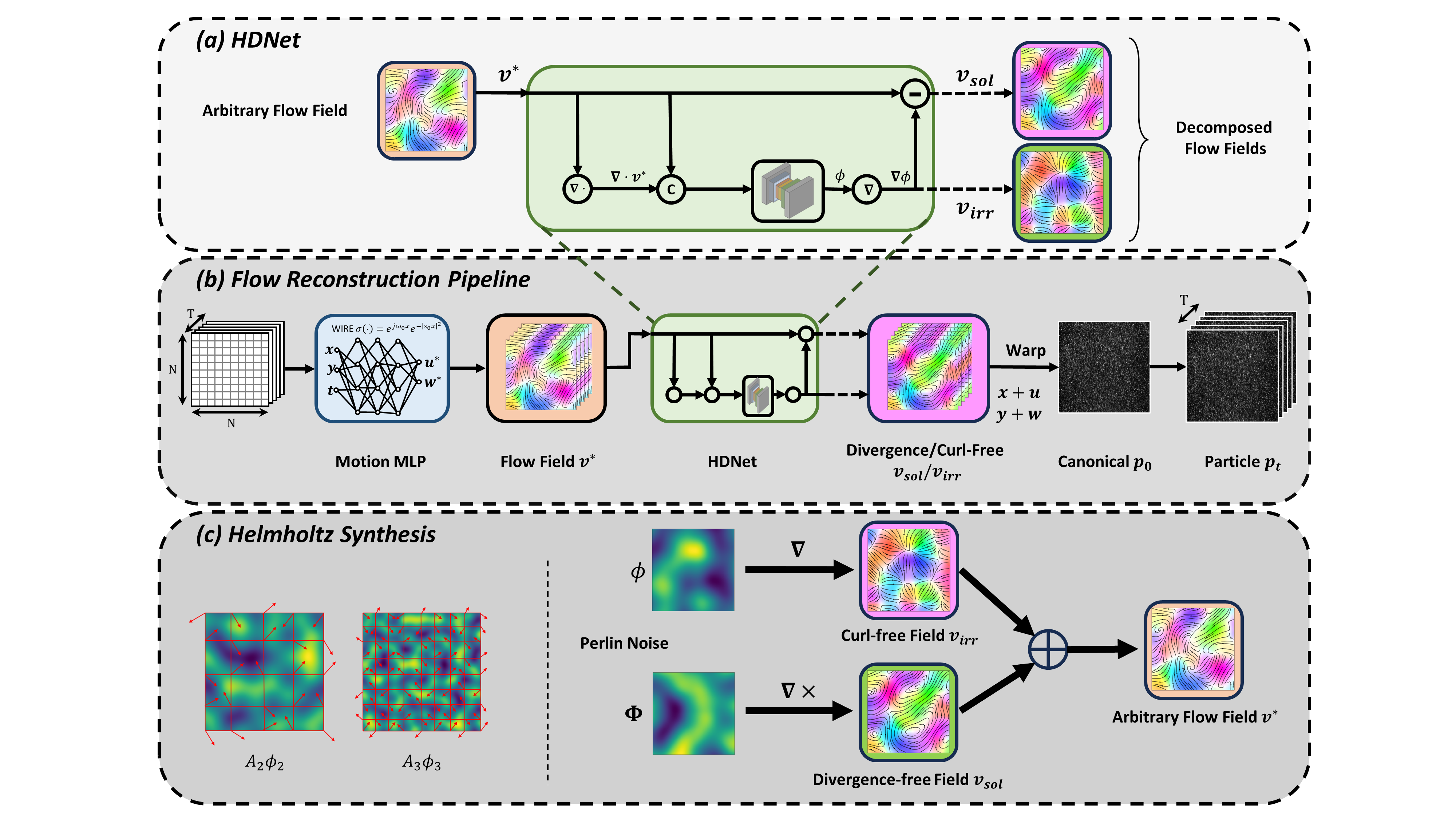
Figure 1: Overview of our pipeline. (a) Concept of HDNet: an arbitrary flow field $\mathbf{v^{*}}$ is decomposed into its irrotational (curl free) and solenoidal (divergence free) components. This is known as a Helmholtz Decomposition (see text for details). (b) An example of how HDNet can be used to enforce the physical properties of vector fields in flow reconstruction problems. A motion MLP is trained to represent the flow of particles in a fluid. The output of the MLP is not necessarily physically plausible. Physical plausibility can be restored by utilizing HDNet to extract the incompressible (i.e. divergence free) component of the flow, which is then used to establish the temporal relationship between the particle fields over time (see Section 5). (c) HDNet is trained exclusively on synthetic data, generated by a reverse process we term “Helmholtz Synthesis”: irrotational and solenoidal components are synthesized from spatially smooth random scalar fields generated with Perlin Noise [7]. They can be combined into general flows $\mathbf{v^{*}}$, forming training pairs with a known Helmholtz decomposition, without requiring costly fluid simulation.

3.1 Helmholtz Decomposition and Physical Interpretation

The key idea behind our approach is to utilize the Helmholtz decomposition of vector fields, which is based on the fundamental theorem of vector calculus. This theorem states that any arbitrary vector field $\mathbf{v}^{*}$ can be decomposed into two orthogonal components: an irrotational (curl-free) and a solenoidal (divergence-free) vector field:

$$\mathbf{v}^{*}=\mathbf{v_{irr}}+\mathbf{v_{sol}}.$$ (1)

Classically, the Helmholtz decomposition is computed by leveraging well-known identities from vector calculus, and then (numerically) solving a Poisson equation. Specifically, any irrotational flow can be expressed as the gradient of a scalar potential field $\phi$:

$$\mathbf{v_{irr}}=\nabla\phi,$$ (2)

Additionally, the curl of a gradient field is equal to zero, as is the divergence of a curl field:

$$\nabla\times(\nabla\phi)=0\quad\quad\mathrm{and}\quad\quad\nabla\cdot(\nabla\times\mathbf{v})=0.$$ (3)

By applying the divergence operator to both sides of Eq. 1, we obtain:

$$\nabla\cdot\mathbf{v}^{*}=\nabla\cdot\mathbf{v_{irr}}+\nabla\cdot\mathbf{v_{sol}}=\nabla\cdot\mathbf{v_{irr}},$$ (4)

which yields the Poisson equation:

$$\nabla\cdot\mathbf{v}^{*}=\nabla^{2}\phi.$$ (5)

Once the potential field $\phi$ is retreived using a Poisson solver, the component fields can be calculated as follows:

$$\mathbf{v_{irr}}=\nabla\phi\quad\quad\mathrm{and}\quad\quad\mathbf{v_{sol}}=\mathbf{v}^{*}-\mathbf{v_{irr}}.$$ (6)

It is important to note that the potential field $\phi$ has physical significance in many different application domains. For example in fluid simulation $\phi=P/\rho$ represents the normalized pressure, where $P$ is the pressure and $\rho$ is the mass density. This term plays a crucial role in the incompressible Navier-Stokes equations, which govern many physical fluid flows. In incompressible fluid simulation, a preliminary flow estimate $\mathbf{v}^{*}$ is often forced to be divergence-free (incompressible) by computing the $\mathbf{v_{sol}}$ term according to Eq. 6, a process commonly known as the pressure projection step.

In some optical applications, such as wavefront sensing [41], phase retrieval [12], or Background-Oriented Schlieren imaging [32], the Helmholtz decomposition takes on another physical interpretation. In these applications, the flow fields correspond to optical flow, which describes how light rays bend due to an optical distortion. This distortion is caused by a spatially varying phase delay in the optical wavefront. The potential field $\phi$ is precisely this phase profile, while the observed optical flow is proportional to its gradient, $\nabla\phi$, making it an irrotational field (see Supplement for details). Therefore, when reconstructing optical flow for an optical distortion inverse problem, it is valid to employ the Helmholtz decomposition to ensure the reconstructed flow is curl-free.

However, the classical Poisson solver approach is not differentiable, making it challenging to integrate into modern PINN pipelines for either forward simulation or inverse reconstruction tasks. With the recent advancements in deep learning, numerous deep learning solvers for PDEs have been proposed [34, 30, 10, 37, 11, 9]. Inspired by these ideas, we propose HDNet (Helmholtz decomposition Network) a novel neural network designed to perform Helmholtz decomposition based on conventional HD (Helmholtz decomposition) operations as described by Eqs.5 and 6.

3.2 HDNet

Architecture.

The HDNet architecture, depicted in Fig. 1 (a), takes as input either an arbitrary flow field or an "initial" estimation of the reconstructed flow. Instead of relying on the commonly used iterative Poisson solver, HDNet employs a deep learning (DL) solver based on a Convolutional Neural Network (CNN) encoder-decoder with a UNet architecture. To mitigate grid artifacts caused by max-pooling layers, we replace them with convolutions with stride, and similarly, we replace all the transpose convolutions with up-sampling layers.

From Equation 5, the input of the network is a general velocity field $\mathbf{v}^{*}$. To facilitate learning of the Helmholtz decomposition, we compute the divergence $\nabla\cdot\mathbf{v}^{*}$, and concatenate it with this input. The UNet core of the HDNet takes this concatenated input and computes the desired potential field $\phi$. From Equations 1 and 3, we can compute the gradient of the output scalar $\nabla\phi$ to get the curl-free component $\mathbf{v_{irr}}$. By subtracting this curl-free component from the input field, we obtain the divergence-free component ($\mathbf{v_{sol}}$).

Training loss.

To train the proposed network, we aim to minimize the discrepancy between the predicted scalar field $\hat{\phi}$ and the ground truth scalar field $\phi$, while simultaneously minimizing the difference between the predicted divergence-free field component ($\mathbf{\hat{v}_{sol}}$) and the ground truth component ($\mathbf{v_{sol}}$). Thus, the training loss is defined as follows:

$$\mathcal{L}=\lVert\mathbf{\hat{v}_{sol}}-\mathbf{v_{sol}}\rVert_{2}^{2}+\lambda_{1}\lVert\hat{\phi}-\phi\rVert_{2}^{2}.$$ (7)

The ground truth $\mathbf{v_{sol}}$ and $\phi$ come from synthesized training data which will be introduced in the following subsection.

3.3 Training Data Generation with Helmholtz Synthesis

To enable supervised training of the network, it is necessary to generate training pairs for HDNet. The training result highly relies on the training dataset quantity and quality. However, conventional commercial fluid simulation software are computationally expensive and time-consuming, limiting the generation of large-scale datasets. To overcome this challenge, we introduce the Helmholtz synthesis module, a novel approach for generating large-scale fluid training datasets. The Helmholtz synthesis module generates data through the reverse process of the Helmholtz decomposition. By exploiting the vector identities in Eq. 3, we can compute irrotational and solenoidal fields from pseudo-random scalar fields and combine them to obtain arbitrary flow fields. To ensure a realistic quality of the generated dataset, we require scalar fields that are smooth, bandwidth-limited, and exhibit large variability, thereby mimicking real-world complexity.

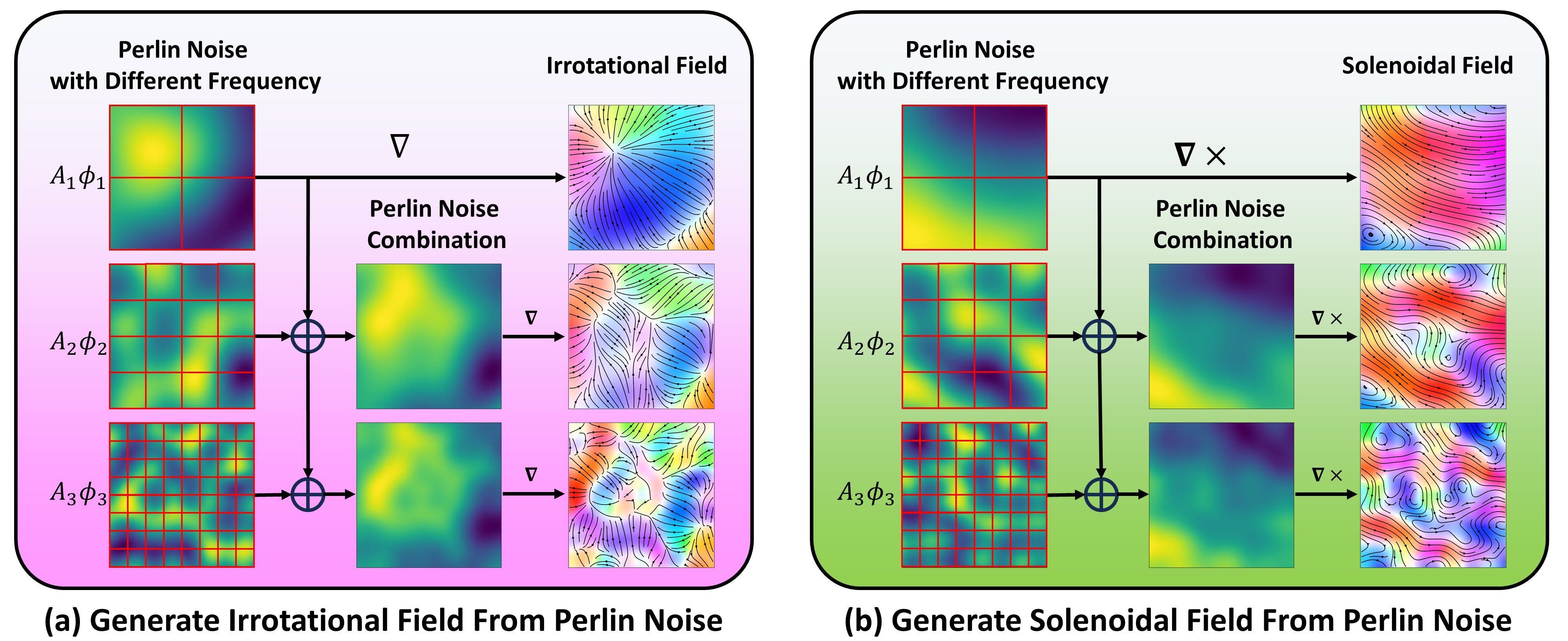
Figure 2: Perlin noise. The red grid in the Perlin noise subfigures controls the Perlin noise frequency. $\phi_{1}$ means with grid $2\times 2$. More grid number means high frequency Perlin noise. (a) is Perlin noise for generating irrotational field. $\mathbf{\nabla}$ mean the gradient of Perlin noise. (b) is for solenoidal field $\mathbf{\nabla\times}$ mean the curl of Perlin noise.

Perlin Noise.

In Computer Graphics, Perlin noise [27] was developed as a way to produce random band-limited scalar fields that satisfy our requirements for spatial smoothness. Different frequency bands of Perlin noise can be composited to generate random patterns of varying spatial detail, known as “turbulence” in the graphics literature. Thus, the pseudo-random generated scalar fields are expressed as: $\phi=\sum A_{n}\phi_{n}$, where $A_{n}=1/{2^{n}}$ is the amplitude of the Perlin noise for the scale $n$, and $\phi_{n}$ is the Perlin noise generated with a $2^{n}\times 2^{n}$ grid. The grid number $2^{n}$ controls the frequency of the generated Perlin noise: the higher the grid number, the higher the frequency of the Perlin noise, and the smaller its amplitude. This amplitude rule is designed in such a way to better simulate natural signals. For example, in Fig.2, $A_{2}\phi_{2}$ denotes a Perlin noise with a grid number of $4$ and an amplitude of $1/4$. While $A_{3}\phi_{3}$ denotes a Perlin noise with a grid number of $8$ and an amplitude of $1/8$.

In our application, we require a Perlin turbulence scalar field $\phi$ to generate the irrotational velocity field. We also need a Perlin turbulence vector field $\mathbf{\Phi}=(\Phi_{1},\Phi_{2},\Phi_{3})$, composed of three Perlin turbulence scalar fields $\Phi_{1},\Phi_{2},\Phi_{3}$, for the generation of the solenoidal velocity field. Therefore, the irrotational and the solenoidal velocity fields are respectively constructed as the gradient of the Perlin noise scalar field [7], and the curl of the Perlin noise vector field:

$$\mathbf{v_{irr}}=\nabla\phi\quad\quad\mathrm{and}\quad\quad\mathbf{v_{sol}}=\nabla\times\mathbf{\Phi}.$$ (8)

Note that for 2D flows, $\mathbf{\Phi}$ degenerates into a scalar field $\Phi$, and the solenoidal velocity field is constructed as:

$$\mathbf{v_{sol}}=(\frac{\partial\Phi}{\partial y},-\frac{\partial\Phi}{\partial x}).$$ (9)

From the vector identities in Eq. 3, we know that the constructed fields satisfy the following properties: $\mathbf{v_{sol}}=\nabla\times\mathbf{\Phi}$ is divergence-free (divergence of curl is zero) and $\mathbf{v_{irr}}=\nabla\phi$ is curl-free (curl of gradient is zero). By combining these two fields, we can obtain an arbitrary flow field using Helmholtz decomposition:

$$\mathbf{v^{*}}=\mathbf{v_{irr}}+\chi\cdot\mathbf{v_{sol}},$$ (10)

where $\chi$ is the weight controlling the relative strengths of the two components.

During the training, we use this generated flow field $\mathbf{v^{*}}$ as the input for our HDNet, while the corresponding divergence-free field $\mathbf{v_{sol}}$ and the scalar field $\phi$ are used as the ground truth of the network. Using this method, we can generate the $20000$ fluid training data pairs with a resolution of $128\times 128$ within approximately half an hour.

4 Application: Use of HDNet for Flow Reconstruction

The proposed HDNet network is versatile and can be incorporated into any differentiable flow simulation or reconstruction pipeline, to enforce hard constraints on the physical properties of the flow in various applications. In this work we are primarily interested in inverse problems that can be expressed as flow estimation tasks. We show quite different applications from fluid flow to optical distortion imaging, all using the same general experimental framework outlined in the following.

Our pipeline consists of a Physics-Informed Neural Network (PINN) for flow reconstruction, as illustrated in Fig. 1 (b). First, we use a coordinate-based MLP network to represent the flow field $\mathbf{v^{*}}=f(x,y,t;\mathbf{\xi})$, where $\mathbf{\xi}$ is the Motion MLP network weight. This network takes as input the spatial and temporal coordinates $(x,y,t)$, and outputs an "initial" reconstructed motion field $\mathbf{v^{*}}=(u^{*},w^{*})$ for each frame.

We employ the Wavelet Implicit neural REpresentation (WIRE) [33] for the Motion MLP, which utilizes a Gabor wavelet as the activation function to learn high-frequency flow motion. Indeed, this activation function has a controllable parameter $\omega_{0}$ that represents the frequency of the signal. By adjusting $\omega_{0}$ during the learning process, we can achieve a coarse-to-fine reconstruction. A smaller $\omega_{0}$ generates smoother results, corresponding to coarse reconstruction, while a larger $\omega_{0}$ generates high-frequency details, corresponding to fine reconstruction. More details about the WIRE representation and the coarse-to-fine reconstruction strategy are respectively discussed in the Supplement Sections D and C.

In the applications we investigate, the reconstructed flows are not arbitrary but exhibit specific physical properties. For example, in the particle imaging velocimetry (PIV) application, the flow of incompressible fluids is divergence-free, while in phase distortion problem imaging, the gradient of the air refractive index reconstruction is curl-free (see Section 3.1). To impose these physical constraints on the initial reconstruction, we apply the pre-trained HDNet to the velocity field $\mathbf{v^{*}}$. The output of the HDNet is the pair of the irrotational and solenoidal fields: $\mathcal{D}(\mathbf{v^{*}})=(\mathbf{v_{sol}},\mathbf{v_{irr}})$. According to the application, we select the component of the velocity that satisfies the physical constraints. Using the HDNet output ($\mathbf{v_{sol}}/\mathbf{v_{irr}}$), we can warp the canonical template field $p_{0}$ to obtain the scene field $p_{t}$ for each frame. Mathematically, this process is expressed as:

$$\hat{p}_{t}(\mathbf{r})=p_{0}(\mathbf{r}+\mathbf{v_{sol/irr}}),$$ (11)

where $\mathbf{r}=(x,y)$ is the spatial coordinates. $\mathbf{v}^{t}_{\mathbf{sol/irr}}$ is the HDNet output: $\mathbf{v_{sol}}$ or $\mathbf{v_{irr}}$ at time $t$. $\hat{p}_{t}(\mathbf{r})$ is the predicted “scene” field at time $t$. It represents the particle density field in the PIV application or the background texture in the case of BOS or wavefront sensor problem. $p_{0}$ is the canonical configuration of the “scene” field. In our framework, we represent this reference configuration using simply a template image, which is a variable to be optimized during the learning process. Eq. 11 is equivalent to the non-linearized brightness consistency [8] in the optical flow problems. Therefore, our pipeline inherently incorporates the non-linearized brightness consistency. Our pipeline is defined as a joint optimization problem, where we aim to retrieve both the canonical scene field and the motion field representation:

$$\mathcal{L}=\operatorname*{arg\,min}_{p_{0},\mathbf{\xi}}\sum_{x,y,t}\lVert p_{0}(\mathbf{r}+\mathcal{D}(f(x,y,t;\mathbf{\xi})))-p_{t}\rVert_{2}^{2}+\lambda_{2}\lVert\nabla_{x,y}\mathcal{D}(f(x,y,t;\mathbf{\xi}))\rVert$$ (12)

The second term corresponds to the total variation (TV) of the velocity field, which promotes smoothness in the velocity field, limiting changes within the neighborhood. $\lambda_{2}$ is the weight of the TV term in the total loss.

5 Experiments

In this section, we demonstrate the application of HDNet within our flow reconstruction pipeline. We first evaluate the reconstruction performance HDNet performance and flow reconstruction pipeline of by using synthetic data in order to assess numerical metrics. Then, we showcase reconstruction outcomes obtained from real PIV, and BOS experimental data, providing visualizations of divergence and curl maps alongside with scalar potential fields. Similar experiments are also presented in the Supplement (Section B.2) for another phase distortion problem: wavefront sensing. The obtained results demonstrate the superior performance of our method in terms of reconstruction quality, physical constraint enforcement, and robustness against noise.

5.1 Synthetic Data

Table 1: MSE value of HDNet inference divergence

	$n=2,\chi=10^{-5}$	$n=3,\chi=10^{-5}$	$n=4,\chi=10^{-5}$	$n=4,\chi=10^{-4}$	$n=4,\chi=10^{-3}$
Mean	$1.4\times 10^{-7}$	$3.87\times 10^{-7}$	$5.71\times 10^{-7}$	$9.31\times 10^{-7}$	$1.24\times 10^{-6}$
Std. Dev.	$6.8\times 10^{-8}$	$7.2\times 10^{-8}$	$4.1\times 10^{-8}$	$1.27\times 10^{-7}$	$2.36\times 10^{-7}$

HDNet evaluation. We demonstrate the performance of HDNet in enforcing incompressibility on the outputed solenoidal field using synthetic data generated by Helmholtz synthesis module. We create five groups of paired datasets, each containing 800 samples, with varying Perlin noise scales $n$ and the weight $\chi$. We assess the divergence of the solenoidal field $\mathbf{v_{sol}}$ output by HDNet and report the mean squared error (MSE) with respect to zero (mean and standard deviation) in Tab. 1.

Flow pipeline evaluation. To quantitatively assess the performance of our flow reconstruction pipeline, we generated synthetic PIV particle image sequences as described in the Supplement B.3. We then compare the predicted flows using different reconstruction methods with the ground truth one.

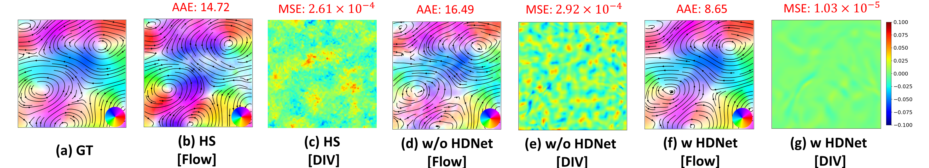
Figure 3: Synthetic PIV data reconstruction comparison. For each method we illustrate the flow field (Flow) and its divergence (DIV). (a) Ground Truth, (b-c) Horn-Schunck optical flow reconstruction, (d-e) our pipeline without HDNet, (f-g) our pipeline with HDNet. We also include quantitative evaluations: AAE (average angular error), and MSE (mean squared error of the divergence).

The results of this comparison are reported in Fig.3. When using our pipeline without HDNet, the reconstruction exhibits significant artifacts and has larger errors than the baseline flow reconstruction using Horn-Schunck [19] optical flow, in both used metrics: AAE (Average Angular Error value) for the flow and the MSE (Mean Square Error) for the divergence. When using the HDNet, our pipeline improves the flow reconstruction with a better AAE, while at the same time reducing the divergence MSE by more than an order of magnitude.

5.2 Real Experiment Data

We also verify our flow reconstruction pipeline in real experiments for both PIV and optical distortion applications. Details of the experimental settings and image sequences can be found in Supplement Section A and Fig. 12.

5.2.1 PIV

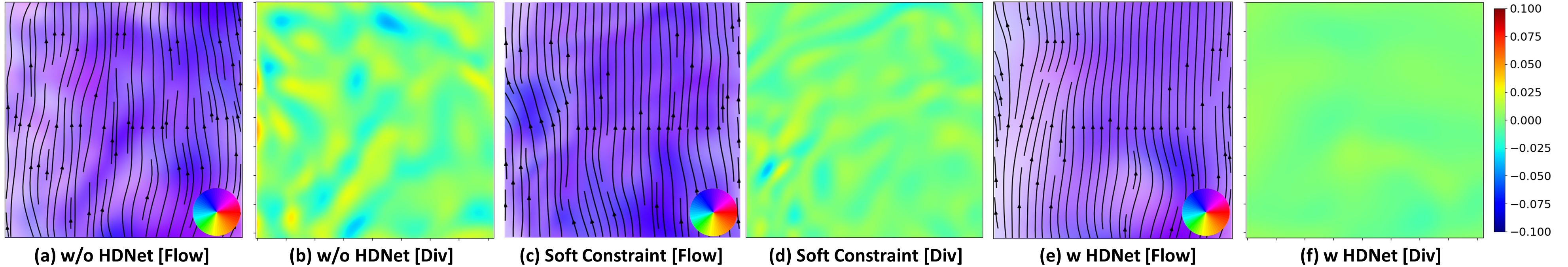
Figure 4: Real PIV data reconstruction comparison. Soft constraint is the method that add a divergence penalty term to the total loss.

Fig. 4 shows the real PIV experiment flow reconstructions. Here, “Soft Constraint” reconstruction consists of adding an $\ell_{2}$ norm of the divergence ($\mathbf{\lVert\nabla\cdot v_{t}}\rVert_{2}^{2}$) to the total loss (Equation 12) to penalize the divergence. It is a very straightforward idea, but the solution does not always satisfy the constraint. From Fig. 4 (d), we can see that there is still some divergence error. With the help of HDNet, our pipeline can reconstruct the flow very well and remove the diverging error. Our method can be thought of as a differentiable hard constraint for the flow reconstruction.

5.2.2 Background-Oriented Schlieren Imaging

In optical distortion applications like BOS, the reconstructed optical flow is the gradient of refractive index (phase) [4], also see Supplement B.1. Therefore, this reconstructed flow should be curl-free (i.e., the curl of the gradient is zero). We compare different methods of reconstruction in Fig.5, and illustrate the reconstructed flows and their corresponding curls .

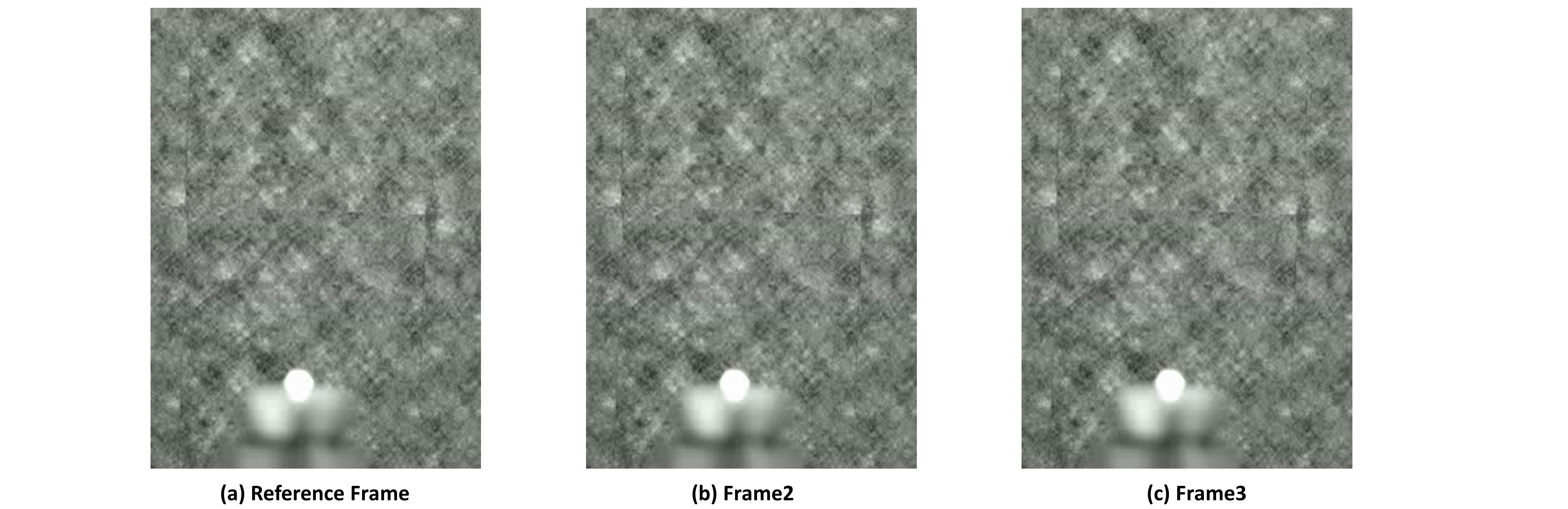
Figure 14: Real experiment BOS image sequence $p_{t}$. This is gas turbulence on a burning candle. The distortion is very tiny.

The flow reconstruction pipeline is similar to the one used for PIV experiments. The only differences are the input images (see Fig. 14 in Supplement), and the use of the $\mathbf{v_{irr}}$ output of HDNet instead of the $\mathbf{v_{sol}}$ output.

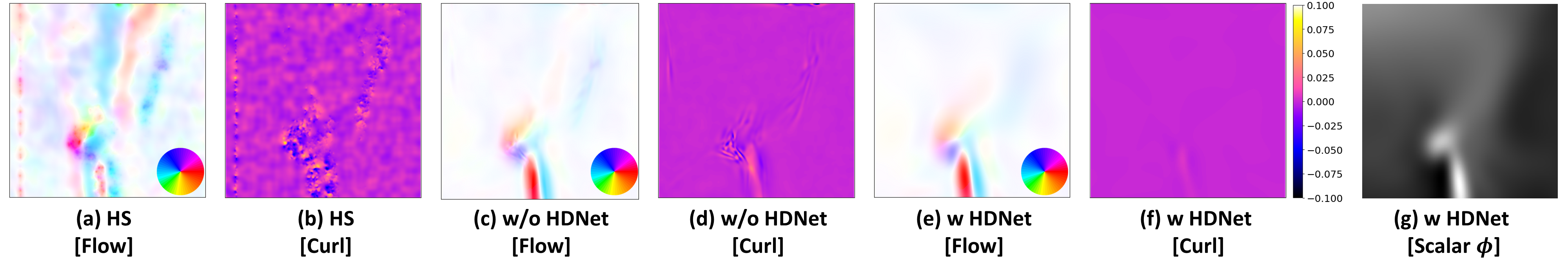
Figure 5: BOS reconstruction comparison. Curl mean the curl value map of left figure. w HDNet scalar $\phi$ means our flow reconstruction pipeline with HDNet and the scalar output of HDNet, that clearly shows the hot air plume above the candle.

The compressed video data used in the original paper [4] exhibits some compression artifacts, leading to noisy flow reconstruction using traditional methods like Horn-Schunck (Fig. 5 (a,b)). Our proposed PINN flow reconstruction pipeline produces a significantly cleaner flow field, effectively removing even the vertical line artifact present in the HS reconstruction Fig. 5 (a-b). Without the use of HDNet, the PINN flow reconstruction pipeline still exhibits a relatively large curl error (see Fig. 5 (d)). By incorporating HDNet, we achieve a significantly smaller curl error Fig. 5 (f), indicating a highly accurate and physically consistent flow reconstruction. Notably, by using HDNet, our method not only reconstructs the flow but also recovers the corresponding phase as illustrated in Fig. 5 (g).

6 Limitations and Future Work

Although HDNet provides a convenient and effective way to inject physical priors into PINNs, the current work has several limitations. First, while the mathematical derivation of the approach holds both in 2D and 3D, currently only the 2D version is implemented. However, the network architecture should be straightforward to adapt to 3D, and since Perlin noise is also defined in 3D, data generation with multi-scale Helmholtz Synthesis is also straightforward. Therefore we do not expect that the generalization of HDNet to 3D will require more than hyperparameter tuning.

A more fundamental limitation is that, as a supervised method, HDNet does not guarantee an exact Helmholtz decomposition of the input flow; in particular the solenoidal component is not guaranteed to be strictly divergence free. The irrotational component is computed as the gradient of an estimated potential field ($\mathbf{v_{irr}}=\nabla\phi$), and is therefore always curl free. However, any mis-estimation of the potential field $\phi$ results in an imprecise decomposition, and thus the calculated solenoidal flow $\mathbf{v_{sol}}=\mathbf{v}^{*}-\mathbf{v_{irr}}$ may still have a remaining divergence component. Our experiments show that this effect is small, however if it is a concern in a particular application, it is also possible to penalize $\nabla\cdot\mathbf{v_{sol}}$ in the loss function for a larger PINN architecture.

7 Conclusion

In this paper, we propose HDNet, a novel network based on the fundamental theorem of vector calculus and Helmholtz decomposition theorem. By employing HDNet, we can effectively impose differentiable hard constraints on inverse imaging problem. We further propose the Helmholtz synthesis module that efficiently generates paired data by reversing Helmholtz decomposition. This module enables the rapid creation of 20000 data pairs within half an hour, making large-scale flow dataset construction feasible and the supervised training of HDNet possible.

Finally, we demonstrate the integration of HDNet into a PINN pipeline for flow reconstruction, showcasing its applicability with examples from PIV and BOS imaging data. Experimental results prove that our HDNet-empowered PINN pipeline outperforms conventional flow reconstruction method. Notably, our approach exhibits versatility and flexibility in satisfying both curl-free and divergence-free constraints while also outputting the scalar potential field.

Appendix A Implementation Details

The HDNet architecture is an MLP with 6 layers, 4 of which are hidden layers. Each hidden layer has 64 neurons. For the WIRE activation functions, the $\omega_{0}$ value ranges from 1.0 to 1.5. $\sigma_{0}$ value ranges from 0.8 to 1.2. We choose the Adam optimizer with learning rate is $1\times 10^{-6}$. We train the HDNet on 20000 data pairs, with 2000 data pairs as the evaluation dataset. Training takes 72 hours on a single A100 GPU. HDNet is applied after 30000 epoch after the coarse reconstruction is almost done.

For the data generation, we use Perlin noise at scales $n$ from 1 to 5. The relative strength of the irrotational and the solenoidal, controlled by the weight $\chi$, can be tuned to the specific application. For example in PIV, the basic Horn Schunck optical flow for an incompressible flow would already have a small divergence that just needs to be reduced further. Therefore we can estimate appropriate weights for the two terms by analyzing the divergence of the basic flow estimate for a representative flow, and choose $\chi$ appropriately. Using this approach, we chose $\chi$ to be a random number from a normal distribution with a mean of 0.0002.

For the full flow estimation pipeline, we chose one of the input frames $p_{0}$ as the template, and initialize accordingly.

Appendix B Experiments

B.1 Phase Distortion Problem Principle

Optical distortion imaging like BOS, wavefront sensing, and phase retrieval can be approached in different ways, but one common approach is to track the apparent motion (optical flow) of a high frequency pattern imaged through the distortion. An example geometry for BOS is shown in Figure 6. The goal of BOS imaging is to measure the phase delay in the distortion plane. A patterned background some distance away is observed with a camera. Since light rays propagate perpendicular to the phase profile $\phi$, the observed optical flow is proportional to the $\nabla\phi$ for small angles (“paraxial approximation”). The factor of proportionality is the propagation distance between the distortion plane and the background.

Because the optical flow is proportional to the phase, the flow is curl free, and the phase actually corresponds to the potential function in the Helmholtz decomposition

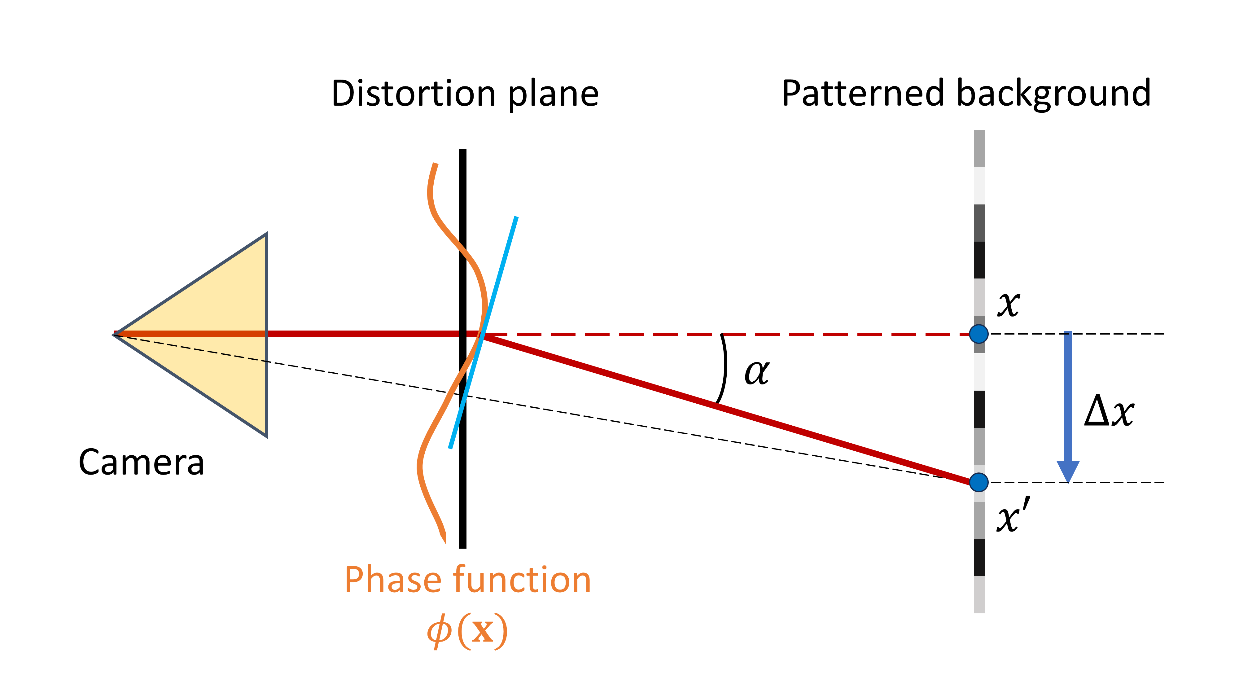
Figure 6: Distortion Imaging Workflow. The camera captures a video sequence of a patterned background through a distortion plane represented by the phase function $\phi(\mathbf{x})$. The patterned background at position $x^{\prime}$ appears distorted to position $x$. Optical flow analysis of the captured video sequence calculates the displacement $\Delta x$, quantifying the distortion. The deflection angle $\alpha$ represents the deviation caused by the distortion plane, and it is proportional to the gradient of the phase $\phi$.

B.2 Wavefront Sensor

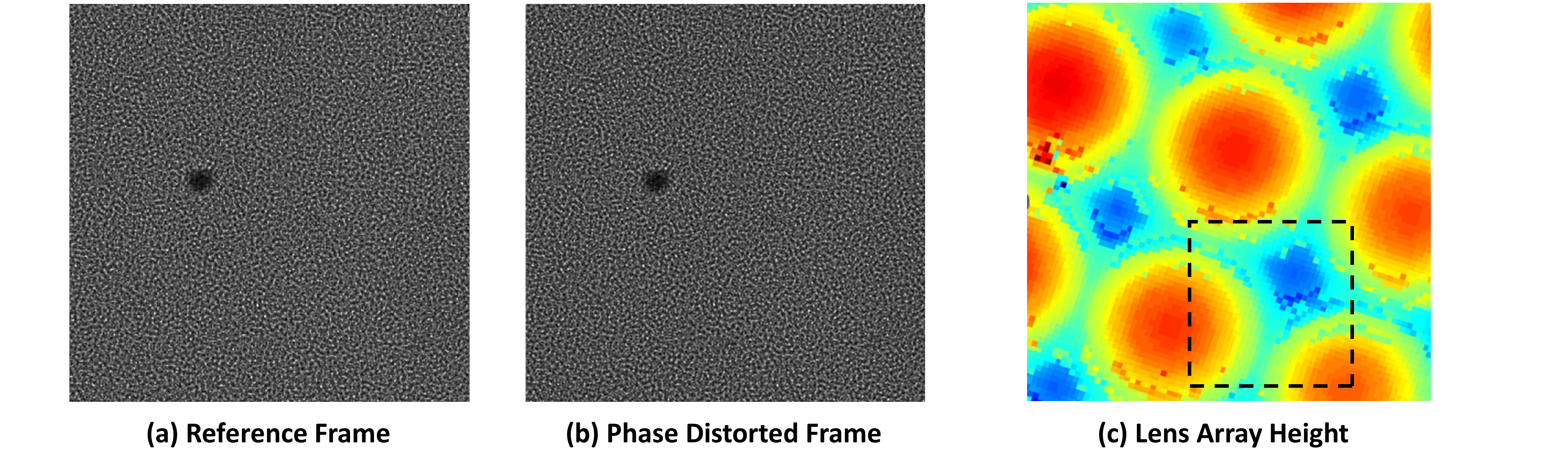
Figure 7: Wavefront sensor captured frames of lens array distortion.

The coded wavefront sensor is also a variant of the classic phase distortion problem [40, 41]. The principle is also similar to what is explained in Section B.1. The distortion is related to the gradient of phase. A mask is placed in the front of the camera. A frame without any distortion is captured as a reference frame (Fig 7 (a)). After the phase lens array (Fig 7 (c)) causing distortion, phase distorted image (Fig 7 (b)) is captured. Fig 7 (c) is a Zygo (interferometric) measurement of the lens array, where the data was provided by the authors of [41].

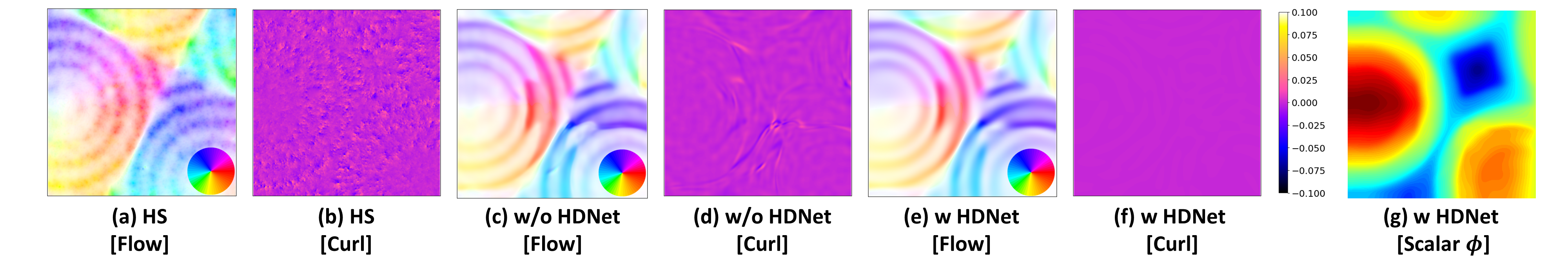
Figure 8: Wavefront sensor lens array reconstruction. This is the reconstruction of lens array. The lens array height is like Fig. 7 (b). It is a regular array of circular lenses separated by symmetrical gaps. (f) is the lens array phase reconstruct.

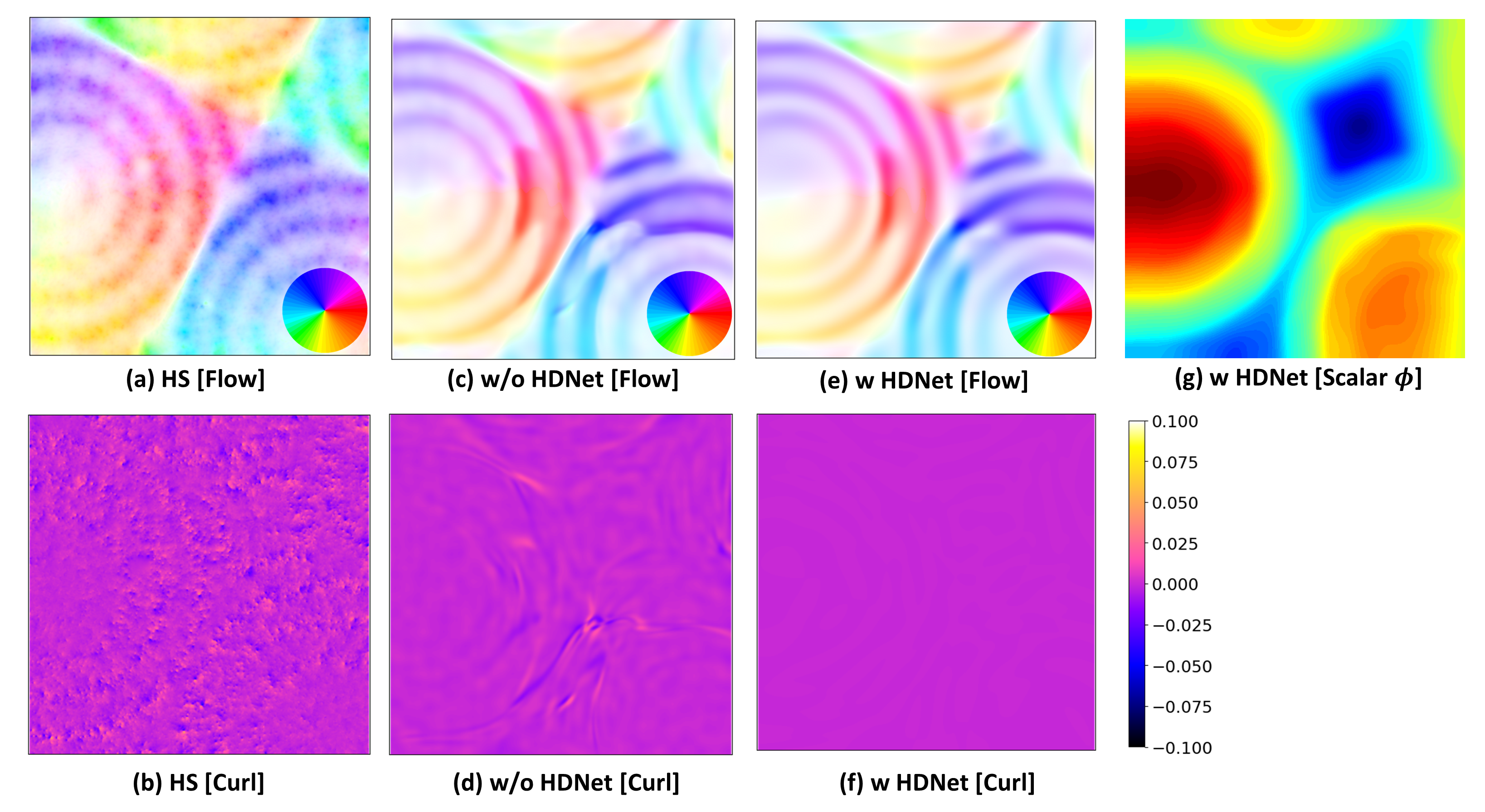
Figure 9: Large figure version of Fig. 8 wavefront sensor lens array reconstruction. This is the reconstruction of lens array. The lens array height is like Fig. 7 (b). It is a regular array of circular lenses separated by symmetrical gaps. (f) is the lens array phase reconstruct.

The reconstruction in Fig. 8 is a crop of the lens array as shown in the black dash square in the Fig. 7 (c). In the unconstrained optical flow measurement we can see that the flow estimates contain erroneous stair-stepping which is not present in the high accuracy interferometric measurements. Comparing (a),(c),(e), we can see that our method has better flow reconstruction quality and fewer artifacts. Comparing (b),(d),(f), we can see that our method have physical constraint performance and curl error value is close to zero. (g) is the phase reconstruction of our method. It is HDNet scalar output. We can see it is symmetrical which match with but have better reconstruction quality than the Zygo measurement in Fig 7 (c).

B.3 PIV Synethetic Data

For the PIV simulations, we first generated 1 frame with 10000 particles in random position with pixels size about 1-2 pixels. The particle pixels value was generated in a normal distribution with mean 1 and variance 0.2. The particle frame figure is shown in Supplement Fig. 10. Then, we used the flow from Helmholtz Synthesis inference dataset to warp the particle to get the other particle image sequence.

Figure 10: Synthetic PIV particle image sequence $p_{t}$

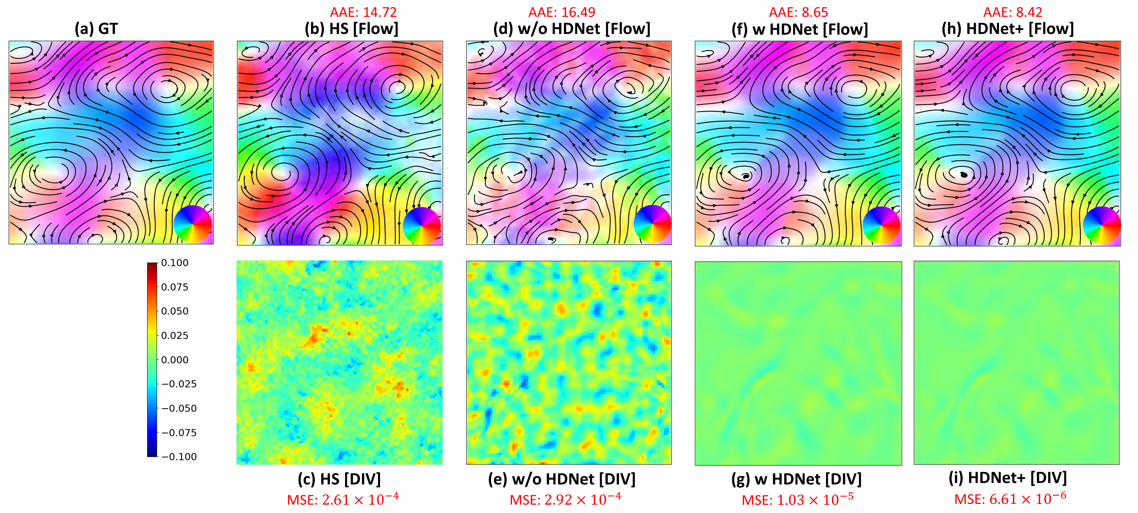
Figure 11: Large figure version of Fig. 3 synthetic PIV data reconstruction comparison. (h) and (i) are the flow and divergence for HDNet+ which is the method that add a divergence penalty term to the total loss to the HDNet flow reconstruction.

HDNet+

It is very straightforward to add a divergence penalty term to the total loss for the flow reconstruction pipeline. To compare with different settings and show the flexibility of HDNet, we also did a comparison experiment that adds a divergence penalty to the total loss for our HDNet flow reconstruction pipeline to explore better reconstruction quality and physical constraint performance. The results are shown in Fig. 11 (h),(i). The reconstruction quality and physical constraint performance are a little bit better.

B.4 PIV Real Experiment Data

The real PIV experiment data is provided to us by [omitted for anonymity]. It is captured with a Phantom2640 camera with a resolution of $1024\times 976$, an exposure time of $99.540~{}\mu s$, and a frame rate of $10000~{}fps$. We cropped the image to have a $256\times 256$ size. Flow particle size is $10~{}\mu m$.

Figure 12: Real experiment PIV particle image sequence $p_{t}$

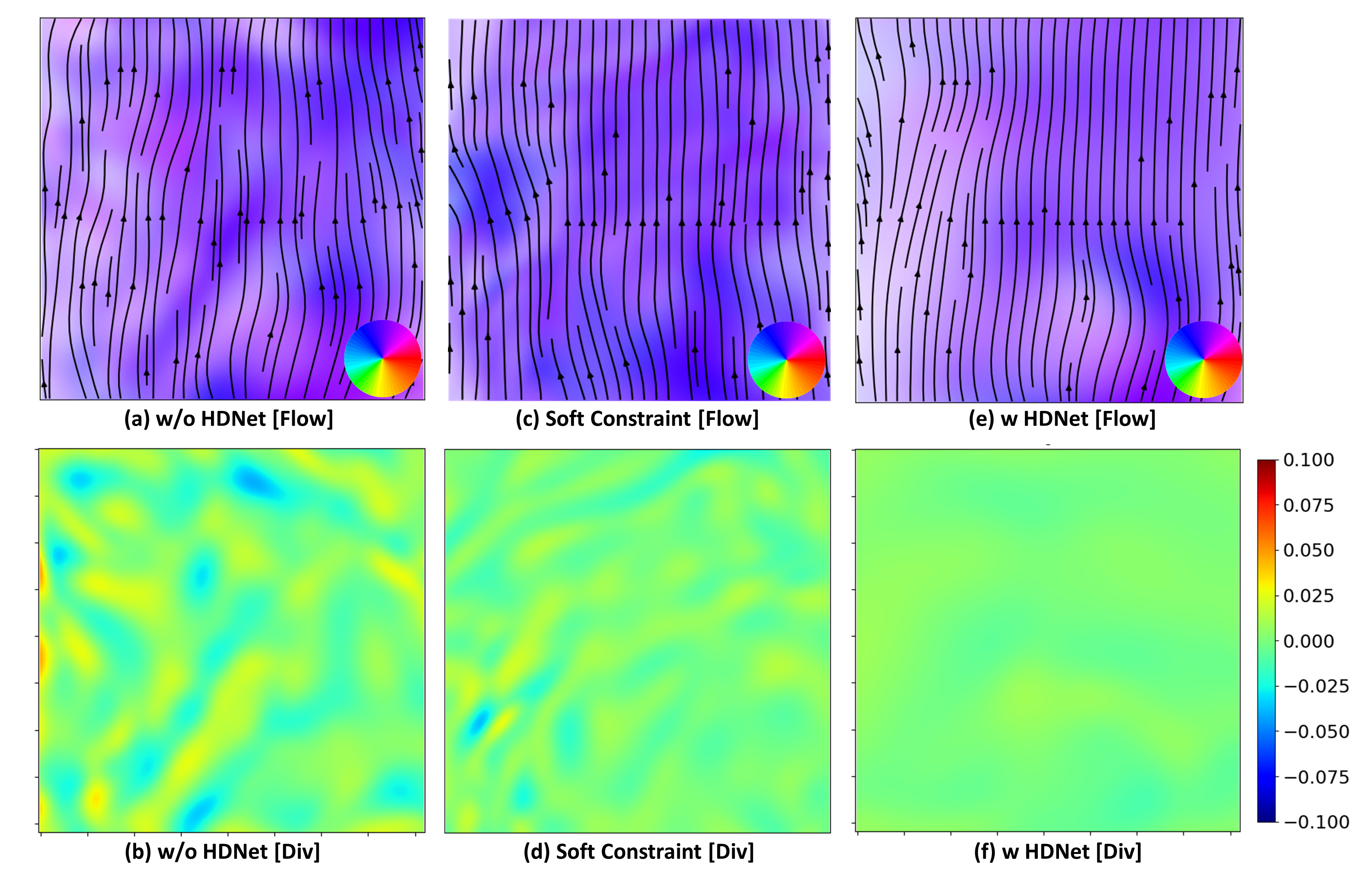
Figure 13: Large figure version of Fig. 4 real PIV data reconstruction comparison. Soft constraint is the method that add a divergence penalty term to the total loss.

B.5 BOS Experiment Data

The data for the BOS experiment is taken from [3] and was provided to us by the authors. The target air distortion for reconstruction is the hot air plume of a burning candle. Image resolution in this case is $270\times 270$. The reconstructed region corresponds to the upper area of the candle hot air. The distortion in these datasets is very small and often only introduces subpixel shifts in the images. The dataset is also particularly challenging since it uses cameras that record a compressed video stream, so that MPEG artifacts further alter the small distortions. The results in the main paper show that HDNet can provide crucial physical regularization to this very difficult inverse problem.

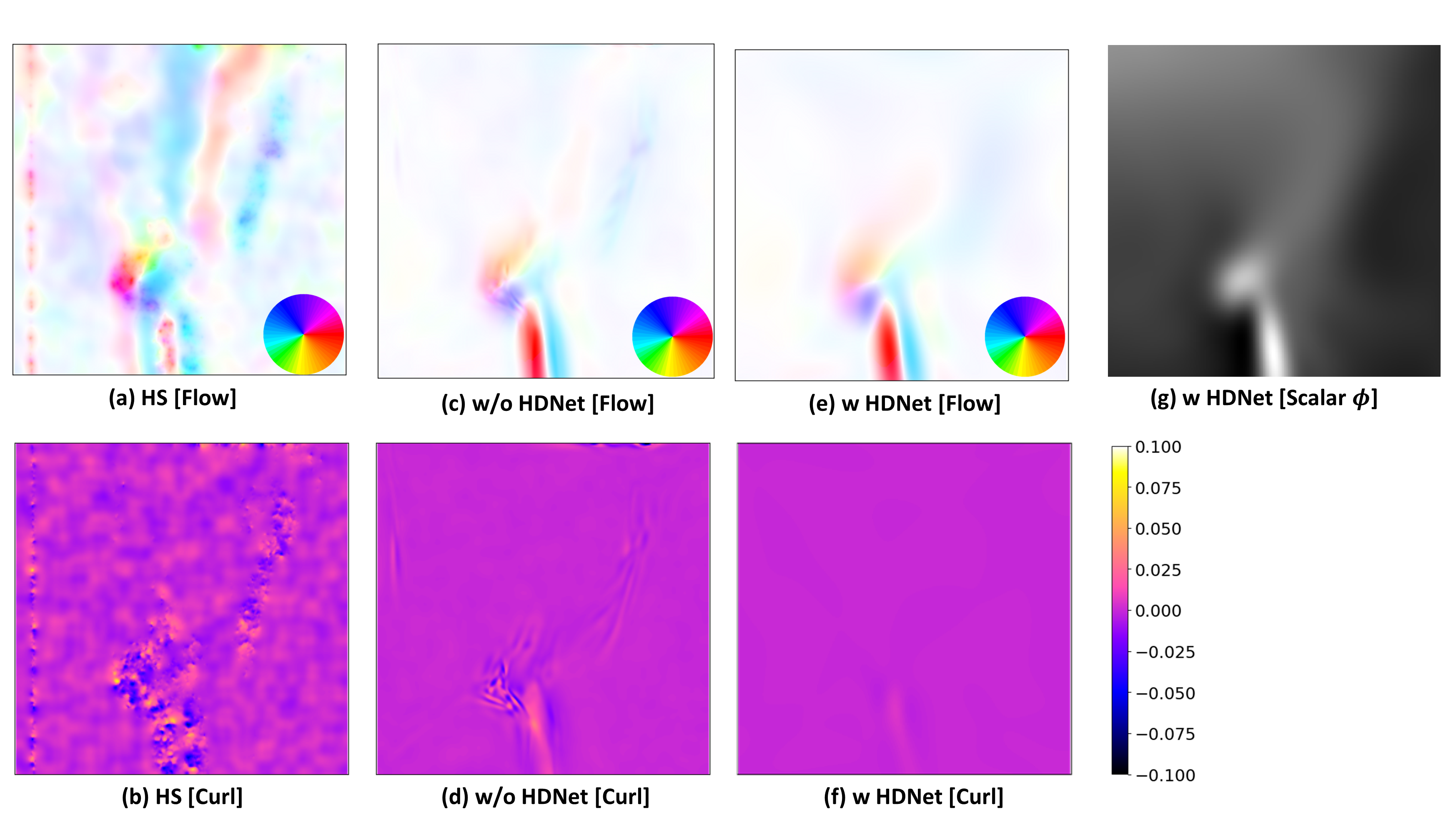
Figure 15: Large figure version of Fig. 5 BOS reconstruction comparison. Curl mean the curl value map of left figure. w HDNet scalar $\phi$ means our flow reconstruction pipeline with HDNet and the scalar output of HDNet, that clearly shows the hot air plume above the candle.

Appendix C Wavelet Implicit Neural Representation

Study reveals that directly learning the image or 2D/3D field with MLP leads to very poor accuracy [36]. One reason is that only the MLP can not learn high frequency of the image. Employing Gabor wavelet as the activation function can enable the MLP to learn the high frequency of the image [33]. Every layer in MLP can be expressed as:

$$\mathbf{y_{m}}=\sigma(W_{m}\mathbf{y_{m-1}+b_{m}}),$$ (13)

where $W_{m},\mathbf{b_{m}}$ are the weight and bias for the m layers [33]; $\sigma$ is the activation function.

$$\sigma(x)=e^{j\omega_{0}x}e^{-|s_{0}x|^{2}}$$ (14)

$\omega_{0}$ determine the frequency level that it represents (Supplement Fig. 16). A smaller $\omega_{0}$ generates smoother results corresponding to the “coarse" reconstruction. A large $\omega_{0}$ generates more high-frequency detail corresponding to “fine" reconstruction. By using this property, we can achieve the coarse-to-fine reconstruction which will be discussed in Supplement Section D.

Adaptive Learnable Parameter Moreover, the WIRE representation exhibits adaptability, as its representation parameters, $\omega_{0}$ and $\sigma_{0}$, are learnable according to the characteristics of the scene being represented. Comparing with NeRF position encoding neural representation, WIRE neural presentation is more continuous for changing the parameter. WIRE is faster than the Fourier Feature [36] and robust for inverse problems of images and video [33].

Appendix D Frequency Coarse to Fine

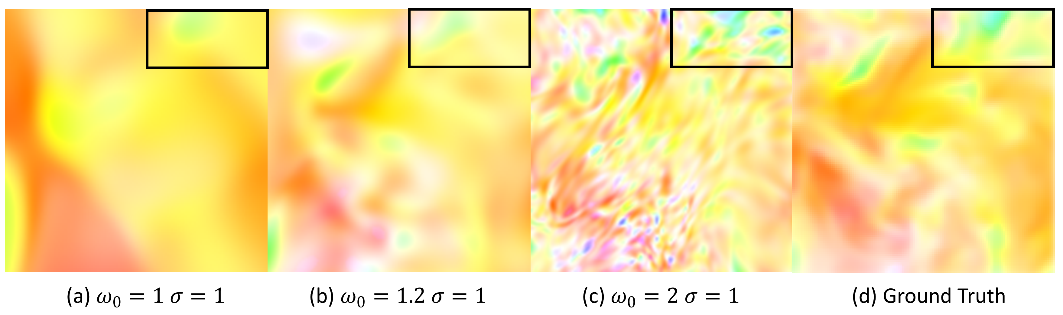
Figure 16: This is the WIRE representation flow reconstruction result with different $\omega_{0}$ and $s_{0}$. A smaller $\omega_{0}$ generates smoother results corresponding to the “coarse" reconstruction. A large $\omega_{0}$ generates more high-frequency detail corresponding to “fine" reconstruction.

Figure 17: Different setup loss figure. We can observe that with a single $w_{0}$ frequency the loss value in the end is always stagnant in a high value. This means the solution is trapped in a local minima. After employing the coarse-to-fine multiscale strategy, the loss decreases to a lower value, which means our coarse-to-fine can overcome the local minima.

There is always a trade-off between achieving accuracy at the local and global levels in flow motion reconstruction. For example, as shown in Supplement Fig. 16, if $w_{0}$ is small, such as $w_{0}=1.2$, the reconstructed flow exhibits an accurate overall shape, but lack the detailed information as shown in Supplement Fig. 16 (b) the black rectangular . Conversely, when $w_{0}$ is too large, such as $w_{0}=2$, there is detail, but the global flow is not correct. This phenomenon arises due to the presence of local minima in the training process for a specific frequency representation (see Supplement Fig. 17 for more detail). To overcome this trade-off we propose a coarse-to-fine approach that starts with low frequency to high frequency.

As discussed in Supplement Section C, small $w_{0}$ means coarse representation and larger $w_{0}$ means fine representation. This property is used to implement the coarse-to-fine strategy. We first start with small $w_{0}$ and then progressively increase $w_{0}$ to a large value as the epoch number increases.

The last step, activating learnability for the parameter $w_{0}$. As explained in the Section C, learnable parameter undergoes automatic fine adjustments based on the scene.

NeurIPS Paper Checklist

1. Claims

2. Question: Do the main claims made in the abstract and introduction accurately reflect the paper’s contributions and scope?

3. Answer: [Yes]

4. Justification: the abstract clearly states the contribution and describes the experimental results.

5. Limitations

6. Question: Does the paper discuss the limitations of the work performed by the authors?

7. Answer: [Yes]

8. Justification: a section on Limitations and Future Work has been included.

9. Theory Assumptions and Proofs

10. Question: For each theoretical result, does the paper provide the full set of assumptions and a complete (and correct) proof?

11. Answer: [N/A]

12. Justification: the paper does not include theoretical results.

13. Experimental Result Reproducibility

14. Question: Does the paper fully disclose all the information needed to reproduce the main experimental results of the paper to the extent that it affects the main claims and/or conclusions of the paper (regardless of whether the code and data are provided or not)?

15. Answer: [Yes]

16. Justification: The method is fully described in the paper and supplement, including the data sources and the synthetic data generation. Full code will be provided with the final paper.

17. Open access to data and code

18. Question: Does the paper provide open access to the data and code, with sufficient instructions to faithfully reproduce the main experimental results, as described in supplemental material?

19. Answer: [No]

20. Justification: it was not possible to anonymize the code and data for public release before the deadline. Both will be released upon acceptance.

21. Experimental Setting/Details

22. Question: Does the paper specify all the training and test details (e.g., data splits, hyperparameters, how they were chosen, type of optimizer, etc.) necessary to understand the results?

23. Answer: [Yes]

24. Justification: Training is described in the main paper with some additional details in the supplement. In addition all code will be provided after acceptance.

25. Experiment Statistical Significance

26. Question: Does the paper report error bars suitably and correctly defined or other appropriate information about the statistical significance of the experiments?

27. Answer: [Yes]

28. Justification: Mean and variance are provided for the HDNet itself. In addition we provide example of applications as individual case studies. These do not have large enough sample size to compute statistics.

29. Experiments Compute Resources

30. Question: For each experiment, does the paper provide sufficient information on the computer resources (type of compute workers, memory, time of execution) needed to reproduce the experiments?

31. Answer: [Yes]

32. Justification: The compute resources (single user workstation) are detailed in the paper.

33. Code Of Ethics

34. Question: Does the research conducted in the paper conform, in every respect, with the NeurIPS Code of Ethics https://neurips.cc/public/EthicsGuidelines?

35. Answer: [Yes]

36. Justification: all guidelines were followed.

37. Broader Impacts

38. Question: Does the paper discuss both potential positive societal impacts and negative societal impacts of the work performed?

39. Answer: [N/A]

40. Justification: flow estimation is a technical problem for many scientific and engineering tasks, but without broad societal impact.

41. Safeguards

42. Question: Does the paper describe safeguards that have been put in place for responsible release of data or models that have a high risk for misuse (e.g., pretrained language models, image generators, or scraped datasets)?

43. Answer: [N/A]

44. Justification: the work poses no risk for misuse.

45. Licenses for existing assets

46. Question: Are the creators or original owners of assets (e.g., code, data, models), used in the paper, properly credited and are the license and terms of use explicitly mentioned and properly respected?

47. Answer: [Yes]

48. Justification: data sources are provided and author permission has been obtained.

49. New Assets

50. Question: Are new assets introduced in the paper well documented and is the documentation provided alongside the assets?

51. Answer: [Yes]

52. Justification: the text contains a full description of the generation of the synthetic training data. Code will also be provided after acceptance.

53. Crowdsourcing and Research with Human Subjects

54. Question: For crowdsourcing experiments and research with human subjects, does the paper include the full text of instructions given to participants and screenshots, if applicable, as well as details about compensation (if any)?

55. Answer: [N/A]

56. Justification: the paper does not involve crowdsourcing nor research with human subjects.

57. Institutional Review Board (IRB) Approvals or Equivalent for Research with Human Subjects

58. Question: Does the paper describe potential risks incurred by study participants, whether such risks were disclosed to the subjects, and whether Institutional Review Board (IRB) approvals (or an equivalent approval/review based on the requirements of your country or institution) were obtained?

59. Answer: [N/A]

60. Justification: the paper does not involve crowdsourcing nor research with human subjects.

References

- [1] Ronald J Adrian and Jerry Westerweel. Particle image velocimetry. Number 30. Cambridge university press, 2011.
- [2] Ekhi Ajuria Illarramendi, Antonio Alguacil, Michaël Bauerheim, Antony Misdariis, Benedicte Cuenot, and Emmanuel Benazera. Towards an hybrid computational strategy based on deep learning for incompressible flows. In AIAA Aviation 2020 Forum, page 3058, 2020.
- [3] Bradley Atcheson, Wolfgang Heidrich, and Ivo Ihrke. An evaluation of optical flow algorithms for background oriented schlieren imaging. Experiments in fluids, 46:467–476, 2009.
- [4] Bradley Atcheson, Ivo Ihrke, Wolfgang Heidrich, Art Tevs, Derek Bradley, Marcus Magnor, and Hans-Peter Seidel. Time-resolved 3d capture of non-stationary gas flows. ACM transactions on graphics (TOG), 27(5):1–9, 2008.
- [5] Daniel M Bear, Elias Wang, Damian Mrowca, Felix J Binder, Hsiao-Yu Fish Tung, RT Pramod, Cameron Holdaway, Sirui Tao, Kevin Smith, Fan-Yun Sun, et al. Physion: Evaluating physical prediction from vision in humans and machines. arXiv preprint arXiv:2106.08261, 2021.
- [6] Amine Bennini, Séphane Lanteri, Frédéric Valentin, Tadeu A Gomes, and Larissa Miguez da Silva. Pinns for the time-domain maxwell equations-preliminary results. In CARLA 2022-Latin America High Performance Computing Conference, 2022.
- [7] Robert Bridson, Jim Houriham, and Marcus Nordenstam. Curl-noise for procedural fluid flow. ACM Transactions on Graphics (ToG), 26(3):46–es, 2007.
- [8] Thomas Brox, Andrés Bruhn, Nils Papenberg, and Joachim Weickert. High accuracy optical flow estimation based on a theory for warping. In Computer Vision-ECCV 2004: 8th European Conference on Computer Vision, Prague, Czech Republic, May 11-14, 2004. Proceedings, Part IV 8, pages 25–36. Springer, 2004.
- [9] Shengze Cai, He Li, Fuyin Zheng, Fang Kong, Ming Dao, George Em Karniadakis, and Subra Suresh. Artificial intelligence velocimetry and microaneurysm-on-a-chip for three-dimensional analysis of blood flow in physiology and disease. Proceedings of the National Academy of Sciences, 118(13):e2100697118, 2021.
- [10] Shengze Cai, Zhiping Mao, Zhicheng Wang, Minglang Yin, and George Em Karniadakis. Physics-informed neural networks (PINNs) for fluid mechanics: A review. Acta Mechanica Sinica, 37(12):1727–1738, 2021.
- [11] Shengze Cai, Zhicheng Wang, Frederik Fuest, Young Jin Jeon, Callum Gray, and George Em Karniadakis. Flow over an espresso cup: inferring 3-d velocity and pressure fields from tomographic background oriented schlieren via physics-informed neural networks. Journal of Fluid Mechanics, 915:A102, 2021.
- [12] Emmanuel J Candes, Yonina C Eldar, Thomas Strohmer, and Vladislav Voroninski. Phase retrieval via matrix completion. SIAM review, 57(2):225–251, 2015.
- [13] Emmanuel J Candes, Xiaodong Li, and Mahdi Soltanolkotabi. Phase retrieval via wirtinger flow: Theory and algorithms. IEEE Transactions on Information Theory, 61(4):1985–2007, 2015.
- [14] Ruiming Cao, Fanglin Linda Liu, Li-Hao Yeh, and Laura Waller. Dynamic structured illumination microscopy with a neural space-time model. In 2022 IEEE International Conference on Computational Photography (ICCP), pages 1–12. IEEE, 2022.
- [15] Ni Chen, Congli Wang, and Wolfgang Heidrich. Snapshot space–time holographic 3d particle tracking velocimetry. Laser & Photonics Reviews, 15(8):2100008, 2021.
- [16] Wenqian Dong, Jie Liu, Zhen Xie, and Dong Li. Adaptive neural network-based approximation to accelerate eulerian fluid simulation. In Proceedings of the International Conference for High Performance Computing, Networking, Storage and Analysis, pages 1–22, 2019.
- [17] Jianguo Du, Guangming Zang, Balaji Mohan, Ramzi Idoughi, Jaeheon Sim, Tiegang Fang, Peter Wonka, Wolfgang Heidrich, and William L Roberts. Study of spray structure from non-flash to flash boiling conditions with space-time tomography. Proceedings of the Combustion Institute, 38(2):3223–3231, 2021.
- [18] James Gregson, Ivo Ihrke, Nils Thuerey, and Wolfgang Heidrich. From capture to simulation: connecting forward and inverse problems in fluids. ACM Transactions on Graphics (TOG), 33(4):1–11, 2014.
- [19] Berthold KP Horn and Brian G Schunck. Determining optical flow. 1980.
- [20] Achuta Kadambi, Celso de Melo, Cho-Jui Hsieh, Mani Srivastava, and Stefano Soatto. Incorporating physics into data-driven computer vision. Nature Machine Intelligence, 5(6):572–580, 2023.
- [21] George Em Karniadakis, Ioannis G Kevrekidis, Lu Lu, Paris Perdikaris, Sifan Wang, and Liu Yang. Physics-informed machine learning. Nature Reviews Physics, 3(6):422–440, 2021.
- [22] John H Lagergren, John T Nardini, Ruth E Baker, Matthew J Simpson, and Kevin B Flores. Biologically-informed neural networks guide mechanistic modeling from sparse experimental data. PLoS computational biology, 16(12):e1008462, 2020.
- [23] GEA Meier. Computerized background-oriented schlieren. Experiments in fluids, 33(1):181–187, 2002.
- [24] Chloé Mimeau and Iraj Mortazavi. A review of vortex methods and their applications: From creation to recent advances. Fluids, 6(2):68, 2021.
- [25] Joseph P Molnar, Lakshmi Venkatakrishnan, Bryan E Schmidt, Timothy A Sipkens, and Samuel J Grauer. Estimating density, velocity, and pressure fields in supersonic flows using physics-informed bos. Experiments in Fluids, 64(1):14, 2023.
- [26] Sang Il Park and Myoung Jun Kim. Vortex fluid for gaseous phenomena. In Proceedings of the 2005 ACM SIGGRAPH/Eurographics symposium on Computer animation, pages 261–270, 2005.
- [27] Ken Perlin. An image synthesizer. ACM Siggraph Computer Graphics, 19(3):287–296, 1985.
- [28] Miao Qi and Wolfgang Heidrich. Scattering-aware holographic piv with physics-based motion priors. In 2023 IEEE International Conference on Computational Photography (ICCP), pages 1–12. IEEE, 2023.
- [29] Markus Raffel, Christian E Willert, Fulvio Scarano, Christian J Kähler, Steve T Wereley, and Jürgen Kompenhans. Particle image velocimetry: a practical guide. Springer, 2018.
- [30] Maziar Raissi, Paris Perdikaris, and George E Karniadakis. Physics-informed neural networks: A deep learning framework for solving forward and inverse problems involving nonlinear partial differential equations. Journal of Computational physics, 378:686–707, 2019.
- [31] Maziar Raissi, Alireza Yazdani, and George Em Karniadakis. Hidden fluid mechanics: Learning velocity and pressure fields from flow visualizations. Science, 367(6481):1026–1030, 2020.
- [32] Hugues Richard and Markus Raffel. Principle and applications of the background oriented schlieren (bos) method. Measurement science and technology, 12(9):1576, 2001.
- [33] Vishwanath Saragadam, Daniel LeJeune, Jasper Tan, Guha Balakrishnan, Ashok Veeraraghavan, and Richard G Baraniuk. Wire: Wavelet implicit neural representations. In Proceedings of the IEEE/CVF Conference on Computer Vision and Pattern Recognition, pages 18507–18516, 2023.
- [34] Justin Sirignano and Konstantinos Spiliopoulos. Dgm: A deep learning algorithm for solving partial differential equations. Journal of computational physics, 375:1339–1364, 2018.
- [35] Barbara Solenthaler and Renato Pajarola. Predictive-corrective incompressible SPH. In ACM SIGGRAPH 2009 papers, pages 1–6. 2009.
- [36] Matthew Tancik, Pratul Srinivasan, Ben Mildenhall, Sara Fridovich-Keil, Nithin Raghavan, Utkarsh Singhal, Ravi Ramamoorthi, Jonathan Barron, and Ren Ng. Fourier features let networks learn high frequency functions in low dimensional domains. Advances in Neural Information Processing Systems, 33:7537–7547, 2020.
- [37] Jonathan Tompson, Kristofer Schlachter, Pablo Sprechmann, and Ken Perlin. Accelerating eulerian fluid simulation with convolutional networks. In International Conference on Machine Learning, pages 3424–3433. PMLR, 2017.
- [38] Benjamin Ummenhofer, Lukas Prantl, Nils Thuerey, and Vladlen Koltun. Lagrangian fluid simulation with continuous convolutions. In International Conference on Learning Representations, 2019.
- [39] Nikolay A Vinnichenko, Aleksei V Pushtaev, Yulia Yu Plaksina, and Alexander V Uvarov. Performance of background oriented schlieren with different background patterns and image processing techniques. Experimental Thermal and Fluid Science, 147:110934, 2023.
- [40] Congli Wang, Qiang Fu, Xiong Dun, and Wolfgang Heidrich. Megapixel adaptive optics: towards correcting large-scale distortions in computational cameras. ACM Transactions on Graphics (TOG), 37(4):1–12, 2018.
- [41] Congli Wang, Qiang Fu, Xiong Dun, and Wolfgang Heidrich. Quantitative phase and intensity microscopy using snapshot white light wavefront sensing. Scientific Reports, 9(1):13795, 2019.
- [42] Hongping Wang, Yi Liu, and Shizhao Wang. Dense velocity reconstruction from particle image velocimetry/particle tracking velocimetry using a physics-informed neural network. Physics of Fluids, 34(1), 2022.
- [43] Jinhui Xiong, Andres Alejandro Aguirre-Pablo, Ramzi Idoughi, Sigurdur T Thoroddsen, and Wolfgang Heidrich. RainbowPIV with improved depth resolution—design and comparative study with TomoPIV. Measurement Science and Technology, 32(2):025401, 2020.
- [44] Jinhui Xiong, Qiang Fu, Ramzi Idoughi, and Wolfgang Heidrich. Reconfigurable rainbow piv for 3d flow measurement. In 2018 IEEE International Conference on Computational Photography (ICCP), pages 1–9. IEEE, 2018.
- [45] Jinhui Xiong, Ramzi Idoughi, Andres A Aguirre-Pablo, Abdulrahman B Aljedaani, Xiong Dun, Qiang Fu, Sigurdur T Thoroddsen, and Wolfgang Heidrich. Rainbow particle imaging velocimetry for dense 3d fluid velocity imaging. ACM Transactions on Graphics (TOG), 36(4):1–14, 2017.
- [46] Guangming Zang, Ramzi Idoughi, Congli Wang, Anthony Bennett, Jianguo Du, Scott Skeen, William L Roberts, Peter Wonka, and Wolfgang Heidrich. Tomofluid: Reconstructing dynamic fluid from sparse view videos. In Proceedings of the IEEE/CVF Conference on Computer Vision and Pattern Recognition, pages 1870–1879, 2020.
- [47] Linfeng Zhang, Jiequn Han, Han Wang, Roberto Car, and Weinan E. Deep potential molecular dynamics: a scalable model with the accuracy of quantum mechanics. Physical review letters, 120(14):143001, 2018.