Surface Operators and Exact Holography

Changha Choi,^a  Jaume Gomis,^a  Raquel Izquierdo García,^a 

^aPerimeter Institute for Theoretical Physics,
Waterloo, Ontario, N2L 2Y5, Canada

Surface operators are nonlocal probes of gauge theories capable of distinguishing phases that are not discernible by the classic Wilson-’t Hooft criterion. We prove that the correlation function of a surface operator with a chiral primary operator in ${\cal N}=4$ super Yang-Mills is a finite polynomial in the Yang-Mills coupling constant. Surprisingly, in spite of these observables receiving nontrivial quantum corrections, we find that these correlation functions are exactly captured in the ’t Hooft limit by supergravity in asymptotically $AdS_{5}\times S^{5}$ [1] ! We also calculate exactly the surface operator vacuum expectation value and the correlator of a surface operator with 1/8-BPS Wilson loops using supersymmetric localization. We demonstrate that these correlation functions in ${\cal N}=4$ SYM realize in a nontrivial fashion the conjectured action of $S$-duality. Finally, we perturbatively quantize ${\cal N}=4$ SYM around the surface operator singularity and identify the Feynman diagrams that when summed over reproduce the exact result obtained by localization.

1. Introduction

In the AdS/CFT correspondence [2, 3, 4] bulk supergravity describes the physics of the boundary field theory in the strong coupling regime. Therefore, there is a priori no reason to expect supergravity to capture the weak coupling expansion of boundary field theory observables that receive quantum corrections.

In this paper we exactly compute correlation functions in ${\cal N}=4$ super-Yang-Mills (SYM) – that in spite of receiving quantum corrections – are exactly captured in the ’t Hooft limit by supergravity in asymptotically $AdS_{5}\times S^{5}$ ! Using our exact results, we demonstrate that these correlation functions in ${\cal N}=4$ SYM realize in a nontrivial fashion the conjectured action of $S$-duality.

The main character in our story are surface operators [5]. These are nonlocal operators in gauge theories that are able to discern between phases of gauge theories that are not otherwise distinguishable by the classic Wilson-’t Hooft criterion [6].

Surface operators in ${\cal N}=4$ SYM are supported on a surface $\Sigma$ in spacetime, which henceforth we take to be the maximally symmetric spaces $\Sigma=\mathbb{R}^{2}$ or $S^{2}$. Surface operators, which we denote by ${\cal O}_{\Sigma}$, are labeled by the choice of a Levi group [5]

$$\mathbb{L}=\prod_{I=1}^{M}U(N_{I})\subset U(N)$$ (1.1)

that specifies how gauge symmetry is broken as the surface $\Sigma$ is approached, and a collection of $4M$ continuous parameters [5]

$$(\alpha_{I},\beta_{I},\gamma_{I},\eta_{I})\,,$$ (1.2)

which are exactly marginal couplings for local operators on the surface defect (surface operators are described in more detail in section 2).

The topologically nontrivial, smooth, asymptotically $AdS_{5}\times S^{5}$ “bubbling” supergravity dual description of surface operators in ${\cal N}=4$ SYM was put forward in [7]. This gave a physical interpretation to the Type IIB supergravity solutions found earlier by Lin-Lunin-Maldacena [8, 9]. The choice of Levi group $\mathbb{L}$ and parameters $(\alpha_{I},\beta_{I},\gamma_{I},\eta_{I})$ that characterize a surface operator in ${\cal N}=4$ SYM are encoded in a nontrivial fashion in the asymptotically $AdS_{5}\times S^{5}$ supergravity solutions [7] (see figure 1 for the dictionary between surface operator data and supergravity solution data).

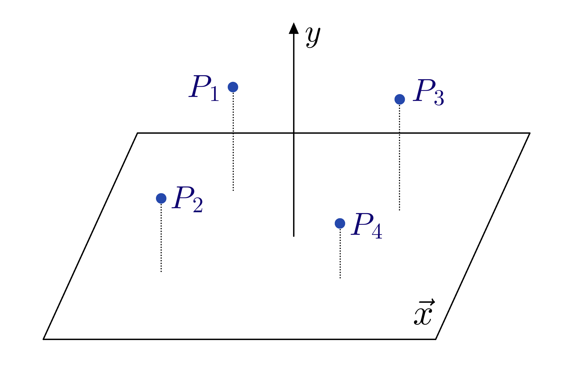
Figure 1: Asymptotically $AdS_{5}\times S^{5}$ solution dual to ${\cal O}_{\Sigma}$ with Levi group $\mathbb{L}=\prod_{I=1}^{M}U(N_{I})$ is determined by $M$ point sources $P_{I}$ that live in a $3d$ half-space $(\vec{x},y\geq 0)$ over which $AdS_{3}\times S^{3}\times S^{1}$ is nontrivially fibered. The mapping of parameters is: $\displaystyle{y_{I}^{2}\over R_{\text{AdS}}^{4}}$ $\displaystyle=N_{I}\qquad\qquad~{}~{}~{}{\vec{x}_{I}\over 2\pi l_{s}^{2}}=(\beta_{I},\gamma_{I})$ $\displaystyle\int_{D_{I}}B_{\text{NS}}$ $\displaystyle=\alpha_{I}\qquad\qquad\int_{D_{I}}B_{\text{R}}=\eta_{I}$ where $D_{I}$ are two-cycles in the asymptotically $AdS_{5}\times S^{5}$ geometry (see [7] for details).

The computation of the correlation functions of a surface operator ${\cal O}_{\Sigma}$ with a chiral primary operator ${\cal O}_{\Delta,k}$ was performed using the dual asymptotically $AdS_{5}\times S^{5}$ supergravity solutions [7] as well as probe D3-branes in [1]. The correlators computed in the supergravity regime, where $\lambda\equiv g^{2}N\gg 1$, take the form [1]

$$\begin{aligned} {\langle{\cal O}_{\Sigma}\cdot{\cal O}_{\Delta,k}\rangle_{\text{sugra}}\over{\langle{\cal O}_{\Sigma}\rangle}_{\text{sugra}}}={1\over\lambda^{|k|\over 2}}\left(A_{0}+{A_{1}\over\lambda}+{A_{2}\over\lambda^{2}}+\ldots{A_{{\Delta-|k|\over 2}}\over\lambda^{{\Delta-|k|\over 2}}}\right)\,,\end{aligned}$$ (1.3)

where $A_{a}$ are explicit functions of $N_{I}$ and of the surface operator parameters $(\beta_{I},\gamma_{I})$.

Instead, in the planar perturbative gauge theory regime, where $\lambda<<1$, the correlator takes the form

$$\begin{aligned} {\langle{\cal O}_{\Sigma}\cdot{\cal O}_{\Delta,k}\rangle_{\text{YM}}\over\langle{\cal O}_{\Sigma}\rangle_{\text{YM}}}={1\over\lambda^{\Delta\over 2}}\left(B_{0}+\sum_{n=1}^{\infty}B_{n}\lambda^{n}\right)\end{aligned}\,.$$ (1.4)

$B_{0}$ was computed in [1] and the following surprise was found: the leading perturbative gauge theory result (1.4) exactly matched the most subleading term in the strong coupling expansion of the supergravity computation (1.3), that is

$$B_{0}=A_{{\Delta-|k|\over 2}}\,.$$ (1.5)

In this paper we compute these correlators using supersymmetric localization, valid at any value of the gauge coupling $g^{2}$, and prove that the perturbative series truncates at a finite order $\left(g^{2}\right)^{{\Delta-|k|\over 2}}$, that is $n_{\text{max}}={\Delta-|k|\over 2}$ in (1.4). This implies that the planar correlator (1.4) terminates and is a polynomial in the coupling

$$\begin{aligned} {\langle{\cal O}_{\Sigma}\cdot{\cal O}_{\Delta,k}\rangle_{\text{YM}}\over\langle{\cal O}_{\Sigma}\rangle_{\text{YM}}}={1\over\lambda^{\Delta\over 2}}\left(B_{0}+B_{1}\lambda+B_{2}\lambda^{2}+\ldots B_{\Delta-|k|\over 2}\lambda^{\Delta-|k|\over 2}\right)\end{aligned}\,.$$ (1.6)

We furthermore show that

$$B_{n}=A_{{\Delta-|k|\over 2}-n}\,,$$ (1.7)

and therefore supergravity computes the planar correlators exactly, even though they acquire quantum corrections!

We also calculate other correlation functions involving surface operators in ${\cal N}=4$ SYM. We exactly determine the vacuum expectation value of a surface operator $\langle{\cal O}_{S^{2}}\rangle$ supported on a two-sphere. The surface operator is also probed with the general ${1/8}$-BPS Wilson-Maldacena loop operator [10, 11, 12, 13, 14] through the correlation function $\langle{\cal O}_{S^{2}}\cdot W^{1/8}_{{\mathcal{R}}}(C)\rangle$, where $C$ is an arbitrary closed curve on a two-sphere that links the surface operator ${\cal O}_{S^{2}}$. Summarizing, we exactly evaluate the following observables:

• $\langle{\cal O}_{S^{2}}\rangle$

• $\langle{\cal O}_{S^{2}}\cdot{\cal O}_{\Delta,k}\rangle$

• $\langle{\cal O}_{S^{2}}\cdot W^{1/8}_{{\mathcal{R}}}(C)\rangle$

Furthermore, we identify the Feynman diagrams that contribute to these correlation functions upon quantizing ${\cal N}=4$ SYM around the surface operator singularity.

A remarkable feature of ${\cal N}=4$ SYM is its conjectured action of $S$-duality. Under the action of an element of the $S$-duality group $PSL(2,\mathbb{Z})$

$${\cal M}=\begin{pmatrix}a&b\\ c&d\end{pmatrix}$$ (1.8)

a surface operator ${\cal O}_{\Sigma}$ is mapped to itself up to a nontrivial action on the parameters [5] (see also [7])

$$\begin{aligned} (\beta_{I},\gamma_{I})\rightarrow|c\tau+d|(\beta_{I},\gamma_{I})\\ (\alpha_{I},\eta_{I})\rightarrow(\alpha_{I},\eta_{I}){\cal M}^{-1}\,,\end{aligned}$$ (1.9)

where

$$\tau={\theta\over 2\pi}+{4\pi i\over g^{2}}$$ (1.10)

is the complexified coupling constant, on which $PSL(2,\mathbb{Z})$ acts as

$$\tau\rightarrow{a\tau+b\over c\tau+d}\,.$$ (1.11)

We demonstrate that $\langle{\cal O}_{S^{2}}\rangle$ and $\langle{\cal O}_{S^{2}}\cdot{\cal O}_{\Delta,k}\rangle$ admit – in a nontrivial fashion – the action of $S$-duality and of the periodic identifications of the surface operator parameters $\alpha_{I}\simeq\alpha_{I}+1$ and $\eta_{I}\simeq\eta_{I}+1$ (see section 2).^,

The plan of the rest of the paper is as follows. In section 2 we discuss surface operators in ${\mathcal{N}}=4$ SYM. In section 3 we explain the implications that conformal anomalies of surface operators have on the expectation value of surface operators. We then compute the expectation value of spherical surface operators using supersymmetric localization in the description of surface operators in terms of coupling $4d$ ${\cal N}=4$ SYM to $2d$ ${\mathcal{N}}=(4,4)$ quiver gauge theories. In section 4 we compute the correlation functions of a surface operator with a chiral primary operator and with a 1/8-BPS Wilson loop by supersymmetric localization on $B^{3}\times S^{1}$ using the disorder definition and suitable supersymmetric boundary conditions and boundary terms. In Appendix A we explain the $B^{3}\times S^{1}$ geometry, and in Appendix B we spell out our conventions on spinors and ${\mathcal{N}}=4$ SYM. In Appendix C we compute $\langle{\mathcal{O}}_{S^{2}}\rangle_{S^{4}}$ using the disorder definition and by localization on $S^{4}$, reproducing the result of section 3. In Appendix D we derive the boundary conditions and the boundary terms describing the surface operators which were used in section 4. In Appendix E and F we perform the perturbative quantization of surface operators in ${\cal N}=4$ SYM using the disorder point of view. We use this to identify the Feynman diagrams that reproduce the exact computations using localization. In Appendix G, we present the explicit computation of the correlation function of a surface operator with a CPO with $\Delta=4,5$.

2. Surface Operators in ${\mathcal{N}}=4$ SYM

A surface operator ${\cal O}_{\Sigma}$ in [5] induces an Aharonov-Bohm phase for a charged particle linking the surface $\Sigma$ (see [22] for a review). This is created by a singular gauge field configuration that breaks the $U(N)$ gauge group to a Levi subgroup $\mathbb{L}=\prod_{I=1}^{M}U(N_{I})\subset U(N)$ as $\Sigma$ is approached. The singularity in the gauge field is given by

$$A=\begin{pmatrix}\alpha_{1}\otimes\mathds{1}_{N_{1}}&0&\ldots&0\\ 0&\alpha_{2}\otimes\mathds{1}_{N_{2}}&\ldots&0\\ \vdots&\vdots&\ddots&\vdots\\ 0&0&\ldots&\alpha_{M}\otimes\mathds{1}_{N_{M}}\end{pmatrix}d\psi\,,$$ (2.1)

where $\psi$ is the (local) angle transverse to the surface $\Sigma$. The parameters $\alpha_{I}\simeq\alpha_{I}+1$ are circle valued, taking values on the maximal torus of $U(N)$.

Since ${\cal O}_{\Sigma}$ breaks $U(N)$ to $\mathbb{L}=\prod_{I=1}^{M}U(N_{I})\subset U(N)$ on the surface, two-dimensional $\theta$-angles can be added on the surface $\Sigma$ for each $U(1)$ factor. These can be combined in an $\mathbb{L}$-invariant matrix

$$\eta=\begin{pmatrix}\eta_{1}\otimes\mathds{1}_{N_{1}}&0&\ldots&0\\ 0&\eta_{2}\otimes\mathds{1}_{N_{2}}&\ldots&0\\ \vdots&\vdots&\ddots&\vdots\\ 0&0&\ldots&\eta_{M}\otimes\mathds{1}_{N_{M}}\end{pmatrix}\,.$$ (2.2)

The parameters $\eta_{I}\simeq\eta_{I}+1$ are also circle valued, taking values on the maximal torus of the $S$-dual or Langlands dual gauge group ${}^{L}G$, where ${}^{L}G=G=U(N)$.

For a maximally supersymmetric surface operator ${\cal O}_{\Sigma}$ in ${\cal N}=4$ SYM, which requires $\Sigma=\mathbb{R}^{2}$ or $S^{2}$, ${\cal O}_{\Sigma}$ induces a codimension two, $\mathbb{L}$-invariant singularity in a complex scalar field $\Phi$

$$\Phi={1\over\sqrt{2}z}\begin{pmatrix}\beta_{1}+i\gamma_{1}\otimes\mathds{1}_{N_{1}}&0&\ldots&0\\ 0&\beta_{2}+i\gamma_{2}\otimes\mathds{1}_{N_{2}}&\ldots&0\\ \vdots&\vdots&\ddots&\vdots\\ 0&0&\ldots&\beta_{M}+i\gamma_{M}\otimes\mathds{1}_{N_{M}}\end{pmatrix}\,,$$ (2.3)

where $z=re^{i\psi}$ is a complex coordinate in the (local) transverse plane to $\Sigma$ and $\Phi={1\over\sqrt{2}}(\phi^{5}+i\phi^{6})$ is a complex scalar made from a choice of 2 out of 6 scalars. The parameters $\beta_{I}$ and $\gamma_{I}$ take values in the Cartan subalgebra of $U(N)$ and are noncompact.

${\cal O}_{\Sigma}$ is thus labeled by a Levi group $\mathbb{L}=\prod_{I=1}^{M}U(N_{I})$ and $4M$ continuous parameters

$$(\alpha_{I},\beta_{I},\gamma_{I},\eta_{I})\,,$$ (2.4)

whose physical interpretation we now elucidate. ${\cal O}_{\Sigma}$ preserves half of the supercharges of ${\cal N}=4$ SYM. Specifically, it preserves $PSU(1,1|2)\times PSU(1,1|2)\times U(1)\subset PSU(2,2|4)$. The $4M$ parameters $(\alpha_{I},\beta_{I},\gamma_{I},\eta_{I})$ are couplings for exactly marginal local operators on the surface defect that when integrated over $\Sigma$ preserve $PSU(1,1|2)\times PSU(1,1|2)\times U(1)$. Explicitly, the corresponding defect operators are:

$$\begin{aligned} \alpha_{I}:&\qquad\text{Tr}F^{I}_{z\overline{z}}\\ \beta_{I}:&\qquad\text{Tr}\left(D_{z}\overline{\Phi}^{I}+D_{\overline{z}}\Phi^{I}\right)\\ \gamma_{I}:&\qquad i\,\text{Tr}\left(D_{z}\overline{\Phi}^{I}-D_{\overline{z}}\Phi^{I}\right)\\ \eta_{I}:&\qquad\text{Tr}F^{I}_{w\overline{w}}\,,\end{aligned}$$ (2.5)

where $I=1,\ldots,M$ and $w$ is a holomorphic coordinate in $\Sigma$. These operators are the top components of two-dimensional $PSU(1,1|2)\times PSU(1,1|2)\times U(1)$ short multiplets.

Alternatively, a surface operator ${\cal O}_{\Sigma}$ can be defined by coupling a $2d$ ${\cal N}=(4,4)$ theory supported on $\Sigma$ to $4d$ ${\cal N}=4$ SYM [5, 25]. The coupling is canonical and is obtained by gauging – in a supersymmetric fashion – the global symmetry of the $2d$ ${\cal N}=(4,4)$ theory with the $4d$ ${\cal N}=4$ SYM gauge group. Integrating out the localized $2d$ fields induces the aforementioned singular field configurations on the ${\cal N}=4$ SYM fields. This presentation of surface operators will be elaborated on in the next section where we compute the expectation value of the surface operator $\langle{\cal O}_{\Sigma}\rangle$.

In this paper we probe ${\cal O}_{\Sigma}$ with local operators and Wilson loop operators. The position dependence of these correlation functions is fixed by conformal invariance. Our goal is to determine the dependence of these correlators on the Levi group $\mathbb{L}$, the parameters $(\alpha_{I},\beta_{I},\gamma_{I},\eta_{I})$ and the Yang-Mills coupling $g^{2}$.

We probe ${\cal O}_{\Sigma}$ with chiral primary operators ${\cal O}_{\Delta}^{A}$, which transform in the $(0,\Delta,0)$ representation of the $SU(4)_{R}$ symmetry. The operators (in the planar normalization) are given by

$${\cal O}_{\Delta}^{A}={(8\pi^{2})^{\Delta/2}\over\lambda^{\Delta/2}\sqrt{\Delta}}C^{A}_{i_{1}\ldots i_{\Delta}}\text{Tr}\left(\phi^{i_{1}}\ldots\phi^{i_{\Delta}}\right)\,,$$ (2.6)

where $Y^{A}=C^{A}_{i_{1}\ldots i_{\Delta}}x^{i_{1}}\ldots x^{i_{\Delta}}$ are $SO(6)$ spherical harmonics and $\lambda=g^{2}N$. Since ${\cal O}_{\Sigma}$ preserves $SO(4)_{R}\subset SU(4)_{R}$, the correlator with a chiral primary is nontrivial only if it is an $SO(4)_{R}$ singlet. For fixed scaling dimension $\Delta$, there are $\Delta+1$ $SO(4)_{R}$ invariant operators ${\cal O}_{\Delta,k}$ labeled by their $U(1)_{R}$ charge $k=-\Delta,-\Delta+2,\ldots,\Delta-2,\Delta$ under the commutant of $SO(4)_{R}$ in $SU(4)_{R}$. The relevant operators that couple to ${\cal O}_{\Sigma}$ are thus

$${\cal O}_{\Delta,k}={(8\pi^{2})^{\Delta/2}\over\lambda^{\Delta/2}\sqrt{\Delta}}C^{\Delta,k}_{i_{1}\ldots i_{\Delta}}\text{Tr}\left(\phi^{i_{1}}\ldots\phi^{i_{\Delta}}\right)\,,$$ (2.7)

where $Y^{A}=C^{\Delta,k}_{i_{1}\ldots i_{\Delta}}x^{i_{1}}\ldots x^{i_{\Delta}}$ are $SO(4)$ invariant spherical harmonics. For concreteness, we explicitly write the first few operators here [1] (see Appendix E)

$$\begin{aligned} {\cal O}_{2,0}&={4\pi^{2}\over\sqrt{6}\lambda}\hbox{Tr}\left(4\Phi\overline{\Phi}-\sum_{I=1}^{4}\phi^{I}\phi^{I}\right);\hskip 46.97505pt{\cal O}_{2,2}={8\pi^{2}\over\sqrt{2}\lambda}\hbox{Tr}\left(\Phi^{2}\right);\cr{\cal O}_{3,1}&={8\pi^{3}\over\lambda^{3/2}}\hbox{Tr}\left(2\Phi^{2}\overline{\Phi}-\Phi\sum_{I=1}^{4}\phi^{I}\phi^{I}\right);\qquad{\cal O}_{3,3}={32\pi^{3}\over\sqrt{6}\lambda^{3/2}}\hbox{Tr}\left(\Phi^{3}\right)\,,\end{aligned}$$ (2.8)

with ${\cal O}_{\Delta,-k}={\overline{\cal O}}_{\Delta,k}$.

The nontrivial correlators in $\mathbb{R}^{4}$ are therefore

$$\langle{\cal O}_{\Sigma}\cdot{\cal O}_{\Delta,k}(x)\rangle={C_{\Delta,k}\over z^{{\Delta+k}\over 2}\overline{z}^{{\Delta-k}\over 2}}\,,$$ (2.9)

with

$$z=\begin{cases}x_{3}+ix_{4}~{}\qquad&\Sigma=\mathbb{R}^{2}\\[4.0pt] -{1\over 2R}({x_{1}^{2}+x_{2}^{2}+x_{3}^{2}+(x_{4}-iR)^{2}})~{}\qquad&\Sigma=S^{2}\end{cases}\,,$$ (2.10)

where the planar defect is at $x_{3}=x_{4}=0$ and $R$ is the radius of $S^{2}$, defined by $\sum_{i=1}^{3}x_{i}^{2}=R^{2}$ and $x_{4}=0$. $U(1)_{R}$ symmetry implies that $C_{\Delta,-k}={\overline{C}}_{\Delta,k}$.

An important operator to probe ${\cal O}_{\Sigma}$ with is the energy-momentum tensor $T_{mn}$. This defines the scaling weight $h$ of surface operator [7], extending the notion of scaling dimension of a local operator to defects [26]. The position dependence is fixed by conformal symmetry. For $\Sigma=\mathbb{R}^{2}$ it takes the form

$${\langle T_{\mu\nu}\cdot{\cal O}_{\Sigma}\rangle\over\langle{\cal O}_{\Sigma}\rangle}=h{\eta_{\mu\nu}\over|z|^{4}},\qquad{\langle T_{ij}\cdot{\cal O}_{\Sigma}\rangle\over\langle{\cal O}_{\Sigma}\rangle}={h\over|z|^{4}}\left[{4n_{i}n_{j}-3\delta_{ij}}\right],\qquad{\langle T_{\mu i}\cdot{\cal O}_{\Sigma}\rangle\over\langle{\cal O}_{\Sigma}\rangle}=0\,,$$ (2.11)

where $x^{\mu}$ are coordinates along $\Sigma=\mathbb{R}^{2}$ and $n^{i}=x^{i}/|z|$ is the unit normal vector to $\Sigma$. $h$ is related by a Ward identity to the correlator with the chiral primary operator ${\cal O}_{2,0}$

$$h=-{N\over 2\pi^{2}\sqrt{6}}\,C_{2,0}\,.$$ (2.12)

This relation is valid for arbitrary $g^{2}$, ${\mathbb{L}}$ and $(\alpha_{I},\beta_{I},\gamma_{I},\eta_{I})$.

3. Surface Operator Expectation Value

In this section we compute the exact expectation value $\langle{\cal O}_{S^{2}}\rangle_{S^{4}}$ of spherical surface operators ${\cal O}_{S^{2}}$ in ${\cal N}=4$ SYM on the four-sphere $S^{4}$. Before delving into the detailed computation, we discuss expectations that stem solely from conformal anomalies.

Conformally invariant surface operators have intrinsic Weyl anomalies [28]. A cohomological analysis implies that there are three parity even Weyl anomalies: $b,c_{1}$ and $c_{2}$ [29]. Given an arbitrary surface $\Sigma$ embedded on a manifold with metric $g_{mn}$, one finds that under a Weyl transformation with parameter $\delta\sigma$

$$\delta_{\sigma}\log\langle{\cal O}_{\Sigma}\rangle={1\over 24\pi}\int d^{2}x\sqrt{h}\delta\sigma\left(bR_{\Sigma}+c_{1}g_{mn}h^{\mu\sigma}h^{\nu\rho}\widehat{K}^{m}_{\mu\nu}\widehat{K}^{n}_{\rho\sigma}-c_{2}W_{\mu\nu\rho\sigma}h^{\mu\rho}h^{\nu\sigma}\right)\,,$$ (3.1)

where $h_{\mu\nu}$, $\widehat{K}^{m}_{\mu\nu}$ and $W_{\mu\nu\rho\sigma}$ are the induced metric on $\Sigma$, the traceless part of extrinsic curvature and pullback of Weyl tensor respectively. The scaling weight $h$ defined in (2.11) can be written in terms of surface Weyl anomalies, as mentioned in [30], and shown in [31, 32]

$$h=-{c_{2}\over 36\pi^{2}}\,,$$ (3.2)

while $c_{1}$ is related to the two-point function of the displacement operator [31, 32]

$$c_{1}={3\pi^{2}\over 4}C_{D}\,.$$ (3.3)

In $\mathbb{R}^{4}$, the geometric invariants (3.1) vanish for $\Sigma=\mathbb{R}^{2}$. For $\Sigma=S^{2}\subset\mathbb{R}^{4}$ or a maximal $S^{2}\subset S^{4}$, the first invariant is nontrivial while the other two vanish. This implies, upon integrating the anomaly, that the expectation value of ${\cal O}_{S^{2}}$ depends on the radius $r$ of $S^{2}$ via

$$\langle{\cal O}_{S^{2}}\rangle_{\mathbb{R}^{4}}\propto\left({r\over r_{0}}\right)^{b/3}\,,$$ (3.4)

where $r_{0}$ is a scheme dependent scale. This means that, in the absence of other symmetries, the finite part of $\langle{\cal O}_{S^{2}}\rangle$ is scheme dependent. $b$ is, however, unambiguous and physical. Indeed, $b$ is monotically decreasing in renormalization group flows triggered by surface defect local operators [33, 34, 35].

Thus far, our discussion of surface operator vacuum expectation values (vev) holds for a generic CFT, that is, for CFTs with no additional spacetime symmetries. We now discuss the salient new features obeyed by the vev of supersymmetric surface operators in ${\cal N}=4$ SYM. Actually, the discussion applies to the vev of any superconformal surface defect in a $4d$ ${\cal N}=2$ SCFT. More precisely the surface defect must preserve a $2d$ ${\cal N}=(2,2)$ superconformal algebra.

Our discussion builds on the work on the $S^{2}$ partition function of $2d$ ${\cal N}=(2,2)$ SCFTs [36, 37, 38]. The dependence of the $S^{2}$ partition function of a generic $2d$ SCFT on exactly marginal couplings $\lambda$ is scheme dependent, as it can be shifted by the local counterterm $\int d^{2}x\sqrt{g}f(\lambda)R$. If the CFT is an ${\cal N}=(2,2)$ SCFT, the counterterms must be supersymmetrized, and the ambiguity of the $S^{2}$ partition function is drastically reduced from an arbitrary function of couplings to a Kähler transformation [15, 16, 18]

$$Z_{S^{2}}\longrightarrow e^{f(t)+\overline{f}(\overline{t})}Z_{S^{2}}\,,$$ (3.5)

where $t$ are exactly marginal couplings that are bottom components of background $2d$ ${\cal N}=(2,2)$ multiplets. Depending on the $SU(2|1)_{A}$ or $SU(2|1)_{B}$ “massive subalgebra” [36, 38] preserved in computing the partition function, $t$ is be either a background twisted chiral multiplet or chiral multiplet. Furthermore, the $S^{4}$ partition function of a $4d$ ${\cal N}=2$ SCFT is also subject to Kähler transformation ambiguities of the exactly marginal couplings $\tau$ [17, 18]

$$Z_{S^{4}}\longrightarrow e^{f(\tau)+\overline{f}(\overline{\tau})}Z_{S^{4}}\,,$$ (3.6)

where, for ${\cal N}=4$ SYM, $\tau$ is the complexified coupling constant (1.10). This implies that the expectation value of an spherical surface operator in $S^{4}$ that preserves ${\cal N}=(2,2)$ superconformal symmetry is well-defined up to Kähler transformations

$$\langle{\cal O}_{S^{2}}\rangle_{S^{4}}\longrightarrow e^{f(t,\tau)+\overline{f}(\overline{t},\overline{\tau})}\langle{\cal O}_{S^{2}}\rangle_{S^{4}}\,.$$ (3.7)

Therefore the vev of a surface operator supported on a maximal $S^{2}\subset S^{4}$ preserving $2d$ ${\cal N}=(2,2)$ superconformal symmetry takes the form

$$\langle{\cal O}_{S^{2}}\rangle_{S^{4}}=\left({r\over r_{0}}\right)^{-4a+b/3}F(t,\tau,\overline{t},\overline{\tau})\,,$$ (3.8)

and is subject to the Kähler transformation (3.7). $b$ is the the Euler surface anomaly we discussed earlier and $a$ is the celebrated $4d$ Euler anomaly, which also decreases along renormalization group flows [39].

In the interest of readers mainly concerned with the physics of $\langle{\cal O}_{S^{2}}\rangle_{S^{4}}$ we present the result now and show the detailed computation below. Explicit computation using $SU(2|1)_{A}$ supersymmetric localization [36, 37] finds

$$\langle{\cal O}_{S^{2}}\rangle_{S^{4}}=\left({r\over r_{0}}\right)^{-\text{dim}\,\mathbb{L}}\left({g^{2}\over 4\pi}\right)^{\text{dim}\,\mathbb{L}/2}e^{-8\pi^{2}\alpha^{2}/g^{2}}\,,$$ (3.9)

where $\alpha$ the matrix in (2.1). $\langle{\cal O}_{S^{2}}\rangle_{S^{4}}$ is one-loop exact, unlike the correlators we study later.

Using that $a=\text{dim}(G)/4$ for $4d$ ${\cal N}=4$ SYM with gauge group $G$, (3.9) implies that the surface operator anomaly $b$ for Levi group $\mathbb{L}$ is [40, 41, 34]

$$b=3\left(\text{dim}\,G-\text{dim}\,\mathbb{L}\right)\,.$$ (3.10)

See also recent work [42].

We now show that $\langle{\cal O}_{S^{2}}\rangle_{S^{4}}$ in (3.9) exhibits the action of $S$-duality as well as the periodicity of the angular variables $(\alpha,\eta)$ of the surface operator in a nontrivial fashion. Since $\langle{\cal O}_{S^{2}}\rangle_{S^{4}}$ is subject to an ambiguity (3.5), we must prove that $\langle{\cal O}_{S^{2}}\rangle_{S^{4}}$ realizes the desired properties up to a Kähler transformation. Here, $t$ are the bottom components of $2d$ ${\cal N}=(2,2)$ background twisted chiral multiplets [43]

$$t=\eta+\tau\alpha\,,$$ (3.11)

where $\tau$ is the complexified $4d$ coupling constant (1.10).

We start by showing the action of the $PSL(2,\mathbb{Z})$ $S$-duality group by looking at its generators $S$ and $T$:

• $S$: $\tau\rightarrow-1/\tau$, which acts as

  $$\begin{aligned} &t\rightarrow-{t\over\tau}\qquad\overline{t}\rightarrow-{\overline{t}\over\tau}\,.\end{aligned}$$ (3.12)

  $\langle{\cal O}_{S^{2}}\rangle_{S^{4}}$ in (3.9) is invariant up to the Kähler transformation $f=-{i\pi t^{2}/\tau}+{1\over 2}\,\text{dim}\,\mathbb{L}\log\tau$.

• $T$: $\tau\rightarrow\tau+1$, which acts as

  $$\begin{aligned} t\rightarrow t+\alpha\qquad\overline{t}\rightarrow\overline{t}+\alpha\,.\end{aligned}$$ (3.13)

  $\langle{\cal O}_{S^{2}}\rangle_{S^{4}}$ in (3.9) is invariant.

Periodicity of the surface operator parameters $(\alpha,\eta)$ is also realized:

• $\alpha\rightarrow\alpha+1$, which acts as

  $$t\rightarrow t+\tau\qquad\overline{t}\rightarrow\overline{t}+\overline{\tau}\,.$$ (3.14)

  $\langle{\cal O}_{S^{2}}\rangle_{S^{4}}$ in (3.9) is periodic up to the Kähler transformation $f=i\pi(2t+\tau)$.

• $\eta\rightarrow\eta+1$, which acts as

  $$t\rightarrow t+1\qquad\overline{t}\rightarrow\overline{t}+1$$ (3.15)

  $\langle{\cal O}_{S^{2}}\rangle_{S^{4}}$ in (3.9) is periodic.

We now proceed to deriving (3.9).

3.1.  $\langle{\cal O}_{S^{2}}\rangle$ from $4d/2d$

${\cal O}_{S^{2}}$ can also be defined by coupling a specific $2d$ ${\cal N}=(4,4)$ quiver gauge theory on $S^{2}$ to ${\cal N}=4$ SYM [5, 25]. The $2d$ gauge theory encodes the choice of Levi group $\mathbb{L}=\prod_{I=1}^{M}U(N_{I})$, where $N=N_{1}+N_{2}+\ldots N_{M}$, in the ranks of the consecutive gauge groups

$$l_{i}=\sum_{j=1}^{i}N_{j}\,.$$ (3.16)

The $2d$ quiver gauge theory can be found in Figure 21. It has ${\cal N}=(4,4)$ supersymmetry, but the quiver is written using ${\cal N}=(2,2)$ multiplets. The Higgs branch of this quiver gauge theory describes the the hyperkähler manifold $T^{*}(U(N)/\mathbb{L})$ in a choice of complex structure. ${\cal N}=4$ SYM is represented in the diagram as an ${\cal N}=2$ vector multiplet coupled to an adjoint hypermultiplet.

The $SU(N)$ flavor symmetry acting on the leftmost $2d$ chiral multiplets is gauged with the ${\cal N}=4$ SYM gauge group in a way that preserves ${\cal N}=(4,4)$ supersymmetry. This induces a superpotential coupling between the leftmost chiral multiplets and one of the chiral multiplets inside the $4d$ adjoint ${\cal N}=2$ hypermultiplet that makes up ${\cal N}=4$ SYM.

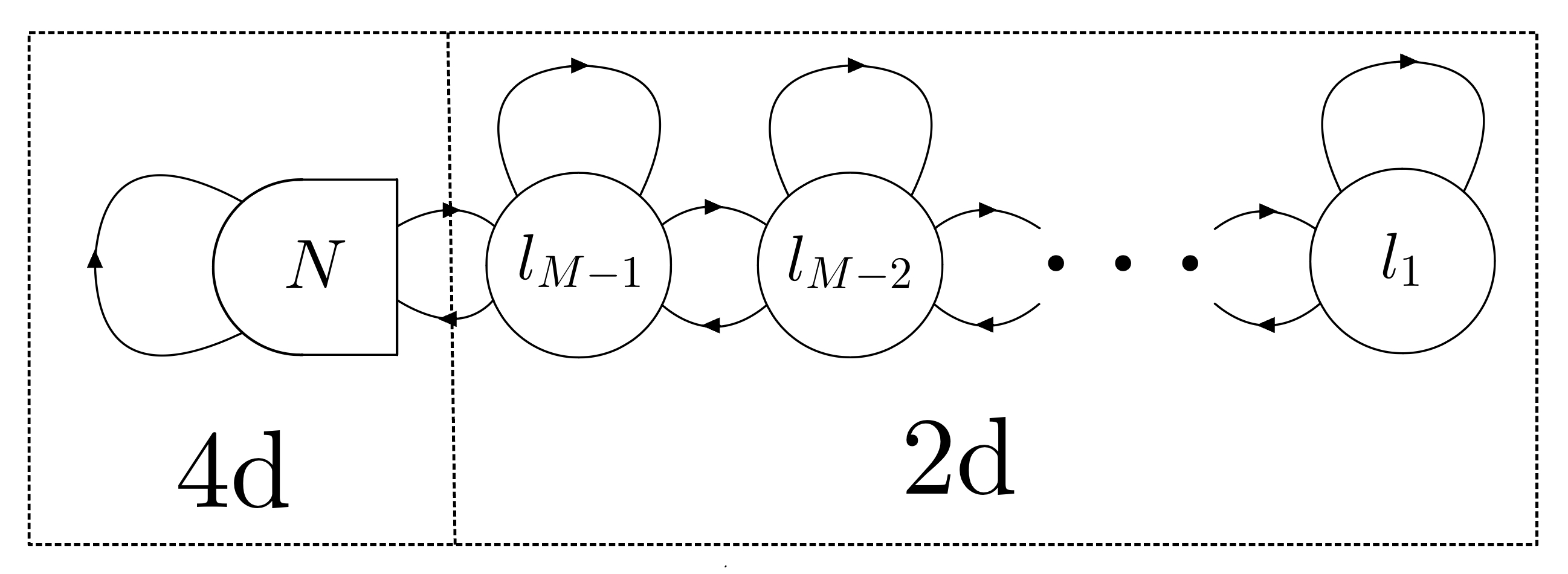
Figure 2: $4d/2d$ quiver description of ${\cal O}_{\Sigma}$.

The parameters $(\alpha_{I},\beta_{I},\gamma_{I},\eta_{I})$ defining ${\cal O}_{\Sigma}$ appear in this description as ${\cal N}=(4,4)$ FI parameters and $2d$ theta angles. In the ${\cal N}=(2,2)$ language the parameters $(\alpha_{I},\beta_{I},\gamma_{I},\eta_{I})$ organize into background chiral and twisted chiral multiplets. They appear in a linear superpotential for each adjoint chiral multiplet and twisted superpotential for each $U(1)$ field strength multiplet.

The computation of $\langle{\cal O}_{S^{2}}\rangle_{S^{4}}$ by supersymmetric localization is a very special convolution of the $S^{4}$ partition function of $4d$ ${\cal N}=2$ theories [46, 47] and the $SU(2|1)_{A}$ invariant $S^{2}$ partition function of $2d$ ${\cal N}=(2,2)$ gauge theories [36, 37]. It takes the form (see also [48, 49, 50, 51])

$$\langle{\cal O}_{S^{2}}\rangle_{S^{4}}=\int da\sum_{B}\int d\sigma Z^{4d}_{\text{cl}}(a)Z^{4d}_{\text{1-loop}}(a)Z^{2d}_{\text{cl}}(\sigma)(a)Z^{2d}_{\text{1-loop}}(\sigma,a)|Z_{\text{inst,vortex}}|^{2}\,.$$ (3.17)

$a$ and $(\sigma,B)$ parametrize $4d$ and $2d$ supersymmetric saddle points of the path integral respectively. $B$ is quantized flux on $S^{2}$, and must be summed over. Then we have the $4d$ and $2d$ classical action and one-loop determinants around the localization locus. $Z_{\text{inst,vortex}}$ is the instanton-vortex partition function (see e.g. [52, 51, 53]). It is determined by the coupling of $4d$ ${\cal N}=4$ SYM to the leftmost chiral multiplets of the $2d$ gauge theory in Figure 21.

We introduce an ${\cal N}=(2,2)$ preserving mass deformation of the $4d/2d$ system by turning on a mass deformation $m$ associated to the $U(1)$ flavor symmetry that is present when the theory is viewed as a $4d$ ${\cal N}=2$ gauge theory coupled to a ${\cal N}=(2,2)$ theory. This describes the coupling of $4d$ ${\cal N}=2^{*}$ to a $2d$ ${\cal N}=(2,2)^{*}$ gauge theory. Setting $m=0$ recovers the half-supersymmetric surface operator in ${\cal N}=4$ SYM.

Let us proceed with the computation by focusing on the $2d$ contribution first. The partition function of the $2d$ gauge theory on $S^{2}$ for general Levi group $\mathbb{L}=\prod_{I=1}^{M}U(N_{I})$ is

$$Z_{2d} ={1\over l_{1}!\,l_{2}!\dots l_{M-1}!}\hskip-3.0pt\sum_{\begin{subarray}{c}B^{(I)}\\ I=1,\dots,M-1\end{subarray}}\int\prod_{I=1}^{M-1}\prod_{s=1}^{l_{I}}{d\sigma_{s}^{(I)}\over 2\pi i}e^{-i4\pi\xi^{(I)}\sigma_{s}^{(I)}-i\theta^{(I)}B_{s}^{(I)}}Z_{vec}Z_{adj}Z_{bf}Z_{f/af}\,.$$ (3.18)

$(\xi^{(I)},\theta^{(I)})$ are FI parameters and $2d$ theta angles that realize the surface operator parameters $(\alpha^{I},\eta^{I}$) and enter the $4d/2d$ theory in twisted superpotentials. The localization one-loop determinants are

$$Z_{vec}=\prod_{I=1}^{M-1}\prod_{s<t}^{l_{I}}\left({(B_{st}^{(I)})^{2}\over 4}+(\sigma_{st}^{(I)})^{2}\right)$$ (3.19)

$$Z_{adj}=\prod_{I=1}^{M-1}\prod_{s\neq t}^{l_{I}}{\Gamma(1-i\sigma_{st}^{(I)}-{B_{st}^{(I)}\over 2}-im)\over\Gamma(i\sigma_{st}^{(I)}-{B_{st}^{(I)}\over 2}+im)}$$

$$Z_{bf}=\prod_{I=1}^{M-2}\prod_{s=1}^{l_{I}}\prod_{t=1}^{l_{I+1}}{\Gamma\left(-i\sigma_{s}^{(I)}+i\sigma_{t}^{(I+1)}-{B_{s}^{(I)}-B_{t}^{(I+1)}\over 2}\right)\Gamma\left(i\sigma_{s}^{(I)}-i\sigma_{t}^{(I+1)}+{B_{s}^{(I)}-B_{t}^{(I+1)}\over 2}+im\right)\over\Gamma\left(1+i\sigma_{s}^{(I)}-i\sigma_{t}^{(I+1)}-{B_{s}^{(I)}-B_{t}^{(I+1)}\over 2}\right)\Gamma\left(1-i\sigma_{s}^{(I)}+i\sigma_{t}^{(I+1)}+{B_{s}^{(I)}-B_{t}^{(I+1)}\over 2}-im\right)}$$

$$Z_{f/af}=\prod_{s=1}^{l_{M-1}}\prod_{t=1}^{N}{\Gamma(-i\sigma_{s}^{M-1}-{B_{s}^{(N-1)\over 2}+ia_{t}})\Gamma(i\sigma_{s}^{M-1}+{B_{s}^{(N-1)\over 2}-ia_{t}}+im)\over\Gamma(1+i\sigma_{s}^{M-1}-{B_{s}^{(N-1)\over 2}-ia_{t}})\Gamma(1-i\sigma_{s}^{M-1}+{B_{s}^{(N-1)\over 2}+ia_{t}}-im)}\,,$$

where we use the notation $x_{st}\equiv x_{s}-x_{t}$. Upon coupling the $2d$ gauge theory to $4d$ ${\cal N}=4$ SYM, the $4d$ Coulomb branch parameters $a$ in the partition function (3.17) appears as twisted masses of the leftmost chiral multiplets. The integration variables $\sigma_{s}^{(I)}$ run just below the real axis and the contour is closed along $\text{Im}(\sigma_{s}^{(I)})<0$.

$Z_{2d}$ can be written as a sum over Higgs vacua [36, 37]. This representation is obtained by summing over the poles

$$Z_{2d}=\sum_{v}Z^{2d}_{\text{cl}}(v)\text{res}_{\sigma=v}\left[Z^{2d}_{\text{1-loop}}(\sigma,a)\right]|Z_{\text{vortex}}|^{2}\,,$$ (3.20)

where $Z_{\text{vortex}}$ is the vortex partition function, which is a nonpertubative contribution.

We first focus on the poles with $B_{s}^{(I)}=0$. The poles with $B_{s}^{(I)}\neq 0$ contribute to $Z_{\text{vortex}}$ [36, 37], to which we turn below. The strategy is to start with the poles of the leftmost chiral multiples and “tie-down” the poles of the other chiral multiplets as we move to the right of the quiver.

From $Z_{f/af}$ we have leading poles of $\{\sigma_{s}^{(M-1)}\}$ which are labeled by $l_{M-1}$-tuples of integers $\vec{k}^{(M-1)}=(k^{(M-1)}_{1},\dots,k^{(M-1)}_{l_{M-1}})$, where $k^{(M-1)}_{i}=1,\dots,l_{M}(=N)$, such that

$$\{\sigma_{s}^{M-1}=a_{k^{(M-1)}_{s}}\}|_{s=1\dots l_{M-1}}\,.$$ (3.21)

Only the mutually distinct poles of $\langle\sigma_{s}^{(M-1)}\rangle$ contribute to the residue because of the zeros from $Z_{vec}$. Since different tuples of $\vec{k}^{(M-1)}$ related by permutations give the same residue, we can remove the $1/l_{M-1}!$ factor in (3.18) and consider ${}_{l_{M}}C_{l_{M-1}}$ possibilities of poles. Therefore, we can treat tuples as a set so that $k^{(M-1)}=\{k_{1}^{(M-1)},\dots,k_{l_{M-1}}^{(M-1)}\}$.

Next, we look at $I=M-2$ part of $Z_{bf}$. Similarly, from $I=M-2$ part of $Z_{bf}$ and $Z_{vec}$, the leading poles of $\{\sigma_{s}^{(M-2)}\}$ are labeled by $l_{M-2}$-tuples without repetitions $\vec{k}^{(M-2)}=(k^{(M-2)}_{1},\dots,k^{(M-2)}_{l_{M-2}})$ such that $\vec{k}^{(M-2)}$ is a subset of $\vec{k}^{(M-1)}$. Similarly, we can remove the $1/l_{M-2}!$ factor by identifying different $\vec{k}^{(M-2)}$ related by permutations and therefore poles are labeled by a set $k^{(M-2)}=\{k_{1}^{(M-2)},\dots,k_{l_{M-2}}^{(M-2)}\}$.

Repeating these steps to the last $I=1$ node, then we see that poles are labeled by a filtration of sets

$$k^{(1)}\subset k^{(2)}\subset\cdots\subset k^{(M-1)}\subset\{1,\dots,N\}\,.$$ (3.22)

Therefore total number of sets of poles are given by

$$\prod_{I=1}^{M-1}{{}_{l_{I+1}}}C_{l_{I}}={N!\over N_{1}!\cdots N_{M}!}\,.$$ (3.23)

It is convenient to realize filtration such that

$$\forall I<J:~{}k_{a}^{(I)}=k_{a}^{(J)},\quad a=1\dots l_{I},\quad I,J=1,\dots,M\,,$$ (3.24)

where we defined $\{k_{a}^{(M)}\}=\{1,\dots,N\}$ with any assignments of the label $a$ where the above filtration is satisfied.

Now, for each set of poles, the residues in (3.20) for each multiplet are (up to an irrelevant numerical factor):

$$\text{res}\,Z^{1-loop}_{vec}=\prod_{I=1}^{M-1}\prod_{s<t}^{l_{I}}\left(a_{k^{(I)}_{s}}-a_{k^{(I)}_{t}}\right)^{2}=\prod_{I=1}^{M-1}\prod_{s\neq t}^{l_{I}}{1\over\gamma\left(ia_{k^{(I)}_{s}}-ia_{k^{(I)}_{t}}\right)}$$ (3.25)

$$\text{res}\,Z^{1-loop}_{adj}=\prod_{I=1}^{M-1}\prod_{s\neq t}^{l_{I}}{1\over\gamma\left(ia_{k^{(I)}_{s}}-ia_{k^{(I)}_{t}}+im\right)}$$

$$\text{res}\,Z_{f/af}^{1-loop}=\prod_{s=1}^{l_{M-1}}\prod_{\begin{subarray}{c}t=1\\ \quad t\neq k_{s}^{(M-1)}\end{subarray}}^{N}\gamma\left(-ia_{k^{(M-1)}_{s}}+ia_{t}\right)\gamma\left(ia_{k^{(M-1)}_{s}}-ia_{t}+im\right)$$

$$\text{res}\,Z_{bf}^{1-loop}=\prod_{I=1}^{M-2}\prod_{s=1}^{l_{I}}\prod_{\begin{subarray}{c}t=1\\ ~{}~{}k_{t}^{(I+1)}\neq k_{s}^{(I)}\end{subarray}}^{l_{I+1}}\gamma\left(-ia_{k^{(I)}_{s}}+ia_{k^{(I+1)}_{t}}\right)\gamma\left(ia_{k^{(I)}_{s}}-ia_{k_{t}^{(I+1)}}+im\right)\,,$$

so that $\text{res}\,Z^{2d}_{\text{1-loop}}$ in (3.20) is

$$\text{res}\,Z^{2d}_{\text{1-loop}}=\text{res}\,Z^{1-loop}_{vec}\cdot\text{res}\,Z^{1-loop}_{adj}\cdot\text{res}\,Z^{1-loop}_{f/af}Z^{1-loop}_{bf}\,,$$ (3.26)

where

$$\gamma(x)\equiv{\Gamma(x)\over\Gamma(1-x)}\,.$$ (3.27)

This can be simplified by embedding $k_{a}^{(I)}$ into $M$-tuples $k_{a}$ such that

$$k_{a}\equiv k_{a}^{(I)},\quad\forall a\leq l_{I},\quad I=1\dots M\,,$$ (3.28)

so the final answer is

$$\text{res}\,Z^{2d}_{\text{1-loop}}=\prod_{I=1}^{M-1}\prod_{s=1}^{l_{M}}\prod_{t=l_{M}+1}^{l_{M+1}}\gamma\left(-i(a_{k_{s}}-a_{k_{t}})\right)\gamma\left(i(a_{k_{s}}-a_{k_{t}}+m)\right)\,.$$ (3.29)

Our main interest is in ${\cal N}=4$ SYM, obtained by setting the ${\cal N}=(2,2)$ mass deformation to vanish, that is $m=0$. For $m=0$ the formula (3.29) simplifies to a ratio of Vandermonde determinants. The numerator is the Vandermonde determinant for the Levi group $\mathbb{L}=\prod_{I=1}^{M}U(N_{I})$ and the denominator the $U(N)$ Vandermonde determinant:

$$\text{res}\,Z^{2d}_{\text{1-loop}}=\prod_{I=1}^{M-1}\prod_{s=1}^{l_{M}}\prod_{t=l_{M}+1}^{l_{M+1}}{1\over(a_{k_{s}}-a_{k_{t}})^{2}}\equiv{\Delta_{\mathbb{L}}(a)\over\Delta_{U(N)}(a)}\,,$$ (3.30)

where

$$\Delta_{\mathbb{L}}(a)=\prod_{\bm{\alpha}>0,\bm{\alpha}\cdot\alpha=0}(\bm{\alpha}\cdot a)^{2}\,,$$ (3.31)

with $\bm{\alpha}$ the roots of the ${\cal N}=4$ SYM gauge group $G$.

The contribution from the poles that arise from $B_{s}^{(I)}\neq 0$ build up the vortex partition function $Z_{\text{vortex}}$ in (3.20). Remarkably, when $m=0$, explicit computation shows that $Z_{\text{vortex}}=1$. This signals the enhancement of supersymmetry and the vanishing contributions in the nontrivial vortex sector is due to fermion zero modes. Likewise, also $Z_{\text{inst,vortex}}=1$ in (3.17) due to the fermion zero modes when $m=0$, where supersymmetry is enhanced (see related discussion in [54] for unramified instantons).

Putting everything together in (3.17) we have therefore shown that

$$\langle{\cal O}_{S^{2}}\rangle_{S^{4}}=\int da\,\Delta_{\mathbb{L}}(a)e^{-{8\pi^{2}\over g^{2}}\left(a^{2}+2ia\alpha\right)}\,,$$ (3.32)

where the $U(N)$ Vandermonde in (3.30) cancels the one-loop determinant of ${\cal N}=4$ SYM. The integral can be evaluated by shifting integration variables

$$a\rightarrow a+i\alpha$$ (3.33)

and using that

$$\Delta_{\mathbb{L}}(a+i\alpha)=\Delta_{\mathbb{L}}(a)\,,$$ (3.34)

as a consequence of $\alpha$ being $\mathbb{L}$-invariant.

Reintroducing the sphere radius dependence by dimensional analysis, sending $a\rightarrow ra$, and performing the integral we get (3.9)

$$\langle{\cal O}_{S^{2}}\rangle_{S^{4}}={r}^{-\text{dim}\,\mathbb{L}}\left({g^{2}\over 4\pi}\right)^{\text{dim}\,\mathbb{L}/2}e^{-8\pi^{2}\alpha^{2}/g^{2}}\,.$$ (3.35)

In Appendix C, we compute $\langle{\cal O}_{S^{2}}\rangle_{S^{4}}$ using the disorder definition of section 2.

4. Surface Operator Correlation Functions Via Localization

In this section we perform a localization computation of non-trivial correlation functions in the presence of surface operators in ${\mathcal{N}}=4$ SYM. We initiate by establishing a geometric framework for localization, followed by the computation of correlation functions involving local chiral primary operators and 1/8-BPS Wilson loops.

4.1.  Geometry of Surface Operator

We perform supersymmetric localization, which we explain in a moment, by placing ${\cal N}=4$ SYM on the conformally flat warped geometry $B^{3}\times S^{1}$ using a Weyl transformation, where $B^{3}$ is a three-dimensional ball. This space is described by coordinates $(\tau,\widetilde{x}_{i})$ with $i=2,3,4$ where $\tau\simeq\tau+2\pi$ and $\widetilde{x}_{i}$ is confined as $\widetilde{x}^{2}\equiv\sum_{i=2}^{4}\widetilde{x}_{i}^{2}\leq R$, and the metric is (this geometry is further explained in Appendix A)

$$ds^{2}(B^{3}\times S^{1})=d\widetilde{x}_{i}^{2}+{R^{2}\over 4}\left(1-{\widetilde{x}^{2}\over R^{2}}\right)^{2}d\tau^{2}\,.$$ (4.1)

From now on, we omit tilde in $\widetilde{x}_{i}$ for clarity. This geometry was originally introduced in [56] to evaluate correlation functions involving 1/8-BPS Wilson loops living on $S^{2}\subset\mathbb{R}^{4}$ [12, 13, 14]. After the Weyl transformation, this $S^{2}$ is mapped to the boundary of $B^{3}$, and the localization computation was performed using a superconformal charge $Q\in PSU(4|4)$. This supercharge generates the $SU(1|1)$ algebra

$$Q^{2}={2\over R}(R_{05}-R_{\tau})\,,$$ (4.2)

where $R_{05}$ is an $SO(2)$ R-symmetry generator which rotates the scalars $(\phi_{0},\phi_{5})$ and $R_{\tau}$ generates $SO(2)$ rotation along $S^{1}$ which shifts $\tau$ (see Appendix B for our conventions for ${\mathcal{N}}=4$ SYM).

The supersymmetry transformation generated by $Q$ is parametrized by a conformal Killing spinor. The conformal Killing spinors on $B^{3}\times S^{1}$ depend on two $Spin(10)$ Weyl spinors $\epsilon_{s}$, $\epsilon_{c}$ of opposite chirality. The explicit expression of conformal Killing spinors on $B^{3}\times S^{1}$ is [57]

$$\epsilon=\cos{\tau\over 2}(\epsilon_{s}+x_{i}\widetilde{\Gamma}^{i}\epsilon_{c})+\sin{\tau\over 2}\widetilde{\Gamma}^{1}(R\epsilon_{c}+{x_{i}\over R}\Gamma^{i}\epsilon_{s})\,.$$ (4.3)

The choice of $\epsilon_{s,c}$ corresponding to $Q$ is

$$\epsilon^{Q}_{s}=\begin{pmatrix}1\\ 0\\ 0\\ 0\end{pmatrix}\otimes\begin{pmatrix}1\\ 0\\ 0\\ 0\end{pmatrix},\quad\epsilon^{Q}_{c}={1\over R}\begin{pmatrix}0\\ 0\\ 0\\ i\end{pmatrix}\otimes\begin{pmatrix}1\\ 0\\ 0\\ 0\end{pmatrix}.$$ (4.4)

Localization of the path integral is then performed by deforming the Euclidean action on $B^{3}\times S^{1}$ by $S\rightarrow S+tQV$ under the condition that $Q^{2}V=0$ and operators inserted are invariant under $Q$. A feature of the choice of $Q$ and $V$ in [56] is that upon reducing fields to the localizing locus $QV=0$, the action becomes a total derivative and hence the path integral reduces to the effective $2d$ theory on $S^{2}$, the boundary of $B^{3}$.

Our main point is that certain correlation functions (namely with local operators and Wilson loops) in the presence of the surface operator ${\cal O}_{\Sigma}$ can be incorporated into the above localization framework and hence can be computed exactly. We achieve this by utilizing the disorder description of the surface operator as described in section 2.

In order to do this, we need to place the surface operator ${\cal O}_{\Sigma}$ on $B^{3}\times S^{1}$ in a way that is compatible with the localizing supercharge $Q$. Namely, we need to insert the surface operator in such a way that it is annihilated by $Q$.

We find that inserting the surface operator ${\cal O}_{\Sigma}$ on $I\times S^{1}\subset B^{3}\times S^{1}$ satisfies the above requirements, where $I$ is any axis of rotation of $B^{3}$ (see also [58]). Using the $SO(3)$ isometry of $B^{3}$, we choose the surface $\Sigma$ to be

$$\Sigma=I\times S^{1}:~{}x_{3}=x_{4}=0,\quad-R\leq x_{2}\leq R,\quad 0\leq\tau\leq 2\pi,$$ (4.5)

where $I$ is an interval passing through the North and South poles of $B^{3}$ (see figure 3). The surface is topologically $\Sigma\simeq S^{2}$, due to the warp factor vanishing at N and S poles (see however discussion at end of section 4.3).

Figure 3: The $B^{3}\times S^{1}$ geometry. The surface operator is supported on $I\times S^{1}$.

The surface operator ${\cal O}_{\Sigma}$ supported on this surface generates the following Q-invariant singular field configurations on $B^{3}\times S^{1}$

$$\Phi=\phi_{w}={\beta+i\gamma\over\sqrt{2}(x_{3}+ix_{4})},\quad\qquad A=\alpha d\psi,$$ (4.6)

where $\phi_{w}={\phi^{7}-i\phi^{8}\over\sqrt{2}}$ and $\psi=\text{arg}(x_{3}+ix_{4})$. This is a simple consequence of the Weyl transformation between $B^{3}\times S^{1}$ and $\mathbb{R}^{4}$ (see Appendix A).

The conformal Killing spinors preserved by the background (4.6), which are solutions to the BPS equations $\delta_{\epsilon}\psi=0$, are characterized by

$$\Gamma^{zw}\epsilon_{s}=0,\quad\widetilde{\Gamma}^{zw}\epsilon_{c}=0\,,$$ (4.7)

where $z=x_{3}+ix_{4}$. This includes the spinor (4.4) which parameterizes the localizing supercharge, and thus the insertion ${\cal O}_{\Sigma}$ is $Q$-invariant.

4.2.  Localization Onto $2d$ Yang-Mills: Review

In this section we review how the localization of ${\mathcal{N}}=4$ SYM on $B^{3}\times S^{1}$ reduces to $2d$ Yang-Mills on $S^{2}=\partial B^{3}$ in the zero-instanton sector [56], which was anticipated in [13, 14]. Throughout the analysis, we set the radius of $B^{3}$ to be $R=1$, and restore $R$ dependence when it is necessary.

The localization is achieved by deforming the Euclidean action $S\rightarrow S+tQV$ with some fermionic field $V$ (see [59] and references therein for an introduction to localization). The choice of fermionic field is given by $V=(\lambda,\overline{Q\lambda})$ where we have the $Spin(10)$ invariant pairing $(\,,):S^{+}\otimes S^{-}\rightarrow\mathbb{C}$ given by $(\chi,\psi)=\sum_{\alpha=1}^{16}\chi_{\alpha}\psi_{\alpha}$. Therefore the deformation term $QV=(Q\lambda,\overline{Q\lambda})$ is positive semi-definite and the localization in the limit of large $t$ makes path integral localize onto the solution of the BPS equations $Q\lambda=0$.

The BPS equations consist of 16 complex (32 real) equations, and we can split $Q\lambda$ into top 8 components $Q\lambda^{t}$ and bottom 8 components $Q\lambda^{b}$ according to the eigenvalues of $-i\Gamma^{0}\Gamma^{1}$. Seven auxiliary fields $K_{I}$ (see [60, 46]) only appear in top equations and we can remove auxiliary fields and remain with 9 real equations from top components where only 8 equations are independent. Then the bottom 16 real equations together with one top equation can be simplified to a constraint that all the bosonic fields be constant along $S^{1}$ up to a gauge transformation, i.e.

$$\partial_{\tau}A_{\mu}=0,\quad\partial_{\tau}\phi_{I}=0\quad\text{(up to gauge transformation)},$$ (4.8)

which is also natural from the fact that $Q^{2}$ generates translation along $\tau$ (4.2). Hence we can effectively focus on the $\tau=0$ slice by assuming all the fields are invariant along $S^{1}$.

The remaining seven real equations in $Q\lambda^{t}$ after imposing (4.8) at $\tau=0$ and resolving the auxiliary fields are given by

$$\text{Re}Q\lambda^{t}|_{e_{k}}= F_{9k}(1-x^{2})-{1\over 2}F_{ij}\epsilon_{ijk}(1+x^{2})+{1\over 2}F_{i+4\,j+4}\epsilon_{ijp}(\delta_{pk}-x^{2}\delta_{pk}+2x_{p}x_{k})$$ (4.9)

$$-F_{5\,j+4}(\delta_{jk}+x^{2}\delta_{jk}-2x_{j}x_{k})+2\phi_{9}x_{k}$$

$$\text{Re}Q\lambda^{t}|_{e_{k+4}}= F_{9\,i+4}(\delta_{ik}+x_{i}x_{k}-x^{2}\delta_{ik})-F_{i5}(\delta_{ik}-x_{i}x_{k}+x^{2}\delta_{ik})+2\phi_{5}(1-x^{2})^{-1}x_{k}$$

$$+F_{i\,j+4}(\varepsilon_{ijk}-x_{i}x_{p}\epsilon_{jpk}-x_{j}x_{p}\epsilon_{ipk})-2\phi_{i+4}\epsilon_{ijk}x_{j}\epsilon_{k+4}$$

$$\text{Re}Q\lambda^{t}|_{e_{5}}= F_{9k}(1-x^{2})-F_{i\,j+4}(\delta_{ij}+\delta_{ij}x^{2}-2x_{i}x_{j})-2\phi_{j+4}x_{j},$$

where $|_{e_{n}}$ means n-th octonion component and $i,j,k,p=2,3,4$ are space indices on $B^{3}$ (see Appendix B).

By looking at the linearized equations of (4.9) around the trivial solution and considering the full equations, it was argued in [56] that $\Phi_{5}=\Phi_{9}=0$ is a solution which is regular at the $S^{2}$ boundary. Together with the $S^{1}$ invariance on the Euclidean ${\cal N}=4$ SYM action, then the bosonic part of the action can be decomposed into a sum of squares of top components BPS equations and a total derivative as

$$S\,\stackrel{{\scriptstyle loc}}{{=}} {2\pi\over 2g^{2}}\int_{B^{3}}d^{3}x\,\left[a_{n}\text{Re}(Q\lambda^{t}|_{e_{n}})^{2}+b_{n}\text{Im}(Q\lambda^{t}|_{e_{n}}x)^{2}\right]$$ (4.10)

$$+{2\pi\over 2g^{2}}\int_{B^{3}}d^{3}x\Big{[}-\nabla_{i}((1-x^{2})(\phi_{i+4}\nabla_{j}\phi_{j+4}-\phi_{j+4}\nabla_{j}\phi_{i+4}))$$

$$\,\quad\quad\quad\quad\quad\quad+4\nabla_{j}(x_{i}x_{k}\phi_{k+4}\nabla_{i}\phi_{j+4}-x_{i}x_{j}\phi_{i}\nabla_{k}\phi_{k+4})$$

$$\,\quad\quad\quad\quad\quad\quad+6\nabla_{j}(x_{i}\phi_{i+4}\phi_{j+4})\Big{]},$$

where the coefficients $a_{n}$, $b_{n}$ can be found in [56]. Therefore, using Stokes theorem, the localized action becomes an effective two-dimensional action on $S^{2}=\partial B^{3}$

$$S_{2d}={\pi\over g^{2}}\int_{S^{2}}d\Omega\left[4\phi_{n}(\nabla_{n}\phi_{n}-\nabla_{i}\phi_{i+4})+6\phi_{n}^{2}\right],$$ (4.11)

where we defined

$$\phi_{n}\equiv n_{i}\phi_{i+4},$$ (4.12)

with $n_{i}=x_{i}/|x_{i}|$. Now the $e_{5}$ part of the localizing equations (4.9) on $S^{2}$ can be simplified to

$$\nabla_{n}\phi_{n}-\nabla_{i}\phi_{i+4}=-\phi_{n},$$ (4.13)

and hence the localized action is reduced to

$$S_{2d}={2\pi\over g^{2}}\int_{S^{2}}d\Omega\,\phi_{n}^{2}.$$ (4.14)

Remarkably, it can be further massaged so that the localizing action can be written as a $2d$ YM theory in the zero-instanton sector. To explain this, let us first introduce a one-form and a connection on $B^{3}$

$$\bm{\phi}\equiv\phi_{i+4}dx^{i},\quad A=A_{i}dx^{i}.$$ (4.15)

Now from the natural inclusion map $\iota:S^{2}\rightarrow B^{3}$, we introduce the pullback of the one-form $\bm{\phi}_{t}=\iota^{*}\bm{\phi}\in\Omega^{1}(S^{2})$ and similarly $A_{t}$. Then there is an identity

$$d_{A}^{*2d}\bm{\phi}_{t}=\nabla_{i}\phi_{i+4}-\nabla_{n}\phi_{n}-2\phi_{n},$$ (4.16)

which together with (4.13) gives

$$S_{2d}={2\pi\over g^{2}}\int_{S^{2}}d\Omega(d^{*2d}_{A}\bm{\phi}_{t})^{2}.$$ (4.17)

Now we define a complex connection $\bm{A}_{\mathbb{C}}$ on $S^{2}$ such that

$$\bm{A}_{\mathbb{C}}=A_{t}-i*_{2d}\bm{\phi}_{t}\equiv A-i*\bm{\phi},$$ (4.18)

where from now on we omit the subscript in $A_{t}$, $\bm{\phi}_{t}$ and $*_{2d}$ by understanding that we are working strictly on $S^{2}$. Now the boundary fields are purely constrained by the tangential part of the localizing equations in (4.9) which are

$$F_{A}-\bm{\phi}\wedge\bm{\phi}=0,\quad d_{A}\bm{\phi}=0.$$ (4.19)

Then we see that

$$\bm{F}_{\mathbb{C}}=F_{A}-\bm{\phi}\wedge\bm{\phi}-id_{A}*\bm{\phi}.$$ (4.20)

Therefore, we see that the $2d$ action becomes a complexified YM action (with an important overall minus sign )

$$S_{2d}=-{1\over g^{2}_{2d^{2}}}\int_{S^{2}}d\Omega\,(*\bm{F}_{\mathbb{C}})^{2},$$ (4.21)

which obeys the two constraints (LABEL:eq:2dconstraints) and the two-dimensional gauge coupling is identified as

$$g^{2}_{2d}=-{g^{2}\over 2\pi R^{2}}.$$ (4.22)

Notice that the two constraints (LABEL:eq:2dconstraints) are two elements of Hitchin equations on $S^{2}$. In fact, it is possible to formulate $2d$ action in terms of constrained Hitchin/Higgs-Yang-Mills theory.

To do that, we briefly review the relevant aspects Hitchin/Higgs-Yang-Mills system following [61]. The field content is given by a gauge field $A$ under compact Lie group $G$ and one form $\phi$ in adjoint representation on a Riemann surface $X$. Then the space of fields $\mathcal{W}=(A,\phi)$ can be regarded as an infinite-dimensional manifold with a natural flat metric induced from $X$

$$g(\delta A_{1},\delta\phi_{1};\delta A_{2},\delta\phi_{2})={1\over 4\pi}\int\delta A_{1}\wedge*\delta A_{2}+\delta\phi_{1}\wedge*\delta\phi_{2}.$$ (4.23)

Moreover, $\mathcal{W}$ is a hyperKähler manifold with three canonical complex structures $I,J,K$ acting on $T^{*}{\mathcal{W}}$ as

$$I^{t}(\delta A)=*\delta A,\quad I^{t}(\delta\phi)=-*\delta\phi$$ (4.24)

$$J^{t}(\delta A)=-\delta\phi,\quad J^{t}(\delta\phi)=\delta A$$

$$K^{t}(\delta A)=-*\delta\phi,\quad K^{t}(\delta\phi)=-*\delta A,$$

which obeys the quaternionic algebra $IJ=-JI=K$, $I^{2}=J^{2}=K^{2}=-1$. The corresponding three natural symplectic structures are

$$w_{I}(\delta A_{1},\delta\phi_{1};\delta A_{2},\delta\phi_{2})={1\over 2\pi}\int_{\Sigma}\delta A_{1}\wedge\delta A_{2}-\delta\phi_{1}\wedge\delta\phi_{2}$$ (4.25)

$$w_{J}(\delta A_{1},\delta\phi_{1};\delta A_{2},\delta\phi_{2})={1\over 2\pi}\int_{\Sigma}\delta A_{1}\wedge*\delta\phi_{2}-\delta A_{2}\wedge*\delta\phi_{1}$$

$$w_{K}(\delta A_{1},\delta\phi_{1};\delta A_{2},\delta\phi_{2})={1\over 2\pi}\int_{\Sigma}\delta A_{1}\wedge\delta\phi_{2}-\delta A_{2}\wedge\delta\phi_{1}.$$

Now there is a natural algebra of vector fields $\mathfrak{g}_{gauge}$ in $\mathcal{W}$ generated by infinitesimal gauge transformations. Then are three natural moment maps $\mu:\mathcal{W}\rightarrow\mathfrak{g}_{gauge}$ corresponding to above symplectic structures given by

$$\mu_{I}(h)=\int(h,F-\phi\wedge\phi)$$ (4.26)

$$\mu_{J}(h)=\int(h,d_{A}*\phi)$$

$$\mu_{K}(h)=\int(h,d_{A}\phi),$$

for any element $\phi\in\mathfrak{g}_{gauge}$.

After this digression, we can write the effective $2d$ path integral as a constrained $2d$ YM theory with gauge group $G_{\mathbb{C}}$ as follows. In terms of $\bm{A}_{\mathbb{C}}=A-i*\bm{\phi}$ and $\bm{F}_{\mathbb{C}}=\mu_{I}-i\mu_{J}$, our path integral is

$$\int_{\mu_{I}=\mu_{K}=0}D\bm{A}_{\mathbb{C}}D\overline{\bm{A}}_{\mathbb{C}}\,e^{{1\over g^{2}_{2d}}\int_{S^{2}}d\Omega\bm{(}*\bm{F}_{\mathbb{C}})^{2}}.$$ (4.27)

Note that while the action itself has $G_{\mathbb{C}}$ gauge symmetry, there is only $G$ gauge symmetry because of the constraint $\mu_{I}=\mu_{K}=0$. The constraints in terms of $\bm{A}_{\mathbb{C}}$ are given by

$$\text{Re}(\bm{F}_{\mathbb{C}})=0,\quad d_{\text{Re}(\bm{A}_{\mathbb{C}})}*\text{Im}(\bm{A}_{\mathbb{C}})=0.$$ (4.28)

Now under the assumption that we can analytically continue the integration contour so that $\text{Re}(\bm{F}_{\mathbb{C}})=\mu_{I}=0$ becomes $\text{Im}(\bm{F}_{\mathbb{C}})=\mu_{J}=0$, we get

$$\int_{\mu_{J}=\mu_{K}=0}D\bm{A}_{\mathbb{C}}D\overline{\bm{A}}_{\mathbb{C}}\,e^{-{1\over g^{2}_{2d}}\int_{S^{2}}d\Omega\bm{\mu}_{I}^{2}}.$$ (4.29)

Of course, the analytic continuation of the contour should be accompanied by the analytic continuation of the coupling $g^{2}_{2d}$.

Focusing on $G=U(N)$, we can plausibly assume that for generic sections of $A$ the solutions of the constraints $\mu_{J}=\mu_{K}=0$ (i.e. $d_{A}\phi=d_{A}^{*}\phi=0$) are trivial such that $\phi=0$. Then we see that the bosonic part of the localized theory is more or less identical to ordinary $2d$ Yang-Mills theory. The standard non-abelian localization argument [62] shows that the path integral of $2d$ Yang-Mills on Riemann surface localized on the instantons which are solutions of the equations of motion $d*F=0$. On $S^{2}$, such instantons are labeled by n-tuples of integers $\{n_{1},\dots,n_{N}\}$ (modulo identifications by the Weyl group). The observation of [56] is that on non-trivial instanton profiles, the kernels of $d_{A}$ and $d_{A}^{*}$ are non-trivial which suggests that the constrained $2d$ Yang-Mills integral (4.29) is subtley different from the ordinary $2d$ Yang-Mills integral. If we additionally assume that the resulting localized path integral (4.29) is equipped with a symplectic measure (LABEL:eq:symplectic_form) with respect to complex structure $I$ and associated with symplectic fermions, then there are non-trivial fermionic zero modes around the non-trivial instantons. This conceptually explains that only the zero-instanton sector contributes to the path integral, and effectively reduces the $2d$ path integral to the ordinary $2d$ YM with zero-instanton sector as

$$\int DA\,e^{-{1\over g^{2}_{2d}}\int_{S^{2}}d\Omega F^{2}}\Big{|}_{\text{0-instanton}}.$$ (4.30)

4.3.  Localization Onto $2d$ Yang-Mills With Surface Operator

The aforementioned localization framework has been successfully applied and tested in various generalizations, see e.g. [63, 64, 65, 66, 67, 58, 68]. Here we extend this localization framework to the case when a surface operator ${\cal O}_{\Sigma}$ is inserted. We take the disorder point of view such that in the path integral description we integrate over fields with desired singular behavior near the surface operator, as in section 2.

In general, the singular behavior of fields produced by disorder operator generates divergences and therefore a proper regularization is needed. One natural choice of regularization is to excise the infinitesimal tubular neighborhood $T$ around the disorder operator. Therefore, the regulated spacetime $T\backslash M$ contains the boundary $\partial T$ and therefore we need additional data at the boundary, which are boundary conditions and possibly boundary terms. In our case of the surface operator in $B^{3}\times S^{1}$, we regularize it by introducing an infinitesimal tube-like cut-off at $\partial M:x_{3}^{2}+x_{4}^{2}=\rho^{2}$ with $\rho\ll 1$ as in figure 4.

To determine them, there are two fundamental guiding principles for the consistency of theory with a boundary (see e.g. [69, 70, 71, 72, 73, 74, 75, 76, 77, 78, 79]). Firstly, the total bulk+boundary action must have a well-defined Euler-Lagrange action principle. Namely, the total bulk+boundary action $S_{tot}$ must obey $\delta S_{tot}=0$ under the bulk Euler-Lagrange equations of motions and the boundary conditions. Secondly, total bulk+boundary action and boundary conditions must be supersymmetric. In Appendix D, we apply these principles to the planar and the spherical surface operator in $\mathbb{R}^{4}$.

Figure 4: The regularized surface operator ${\cal O}_{\Sigma}$ on $B^{3}$, where the boundary is an infinitesimal tube with radius $\rho$.

Based on the successful story of the planar and the spherical surface operators in $\mathbb{R}^{4}$ described in the Appendix D, we streamline the determination of boundary conditions and the supersymmetric boundary term in $B^{3}\times S^{1}$. We introduce labels $i,j,\dots=1,2$,  $a,b,\dots=3,4$,  $I,J,\dots=5,6,9,0$,  $\widehat{A},\widehat{B},\dots=7,8$.

Recalling (4.3), the conformal Killing spinors on $B^{3}\times S^{1}$ satisfying $\nabla_{\mu}=\widetilde{\Gamma}_{\mu}\widetilde{\epsilon}$ are given by

$$\epsilon =(\cos{\tau\over 2}+\sin{\tau\over 2}{x_{i}\over R}\widetilde{\Gamma}^{1}\Gamma^{i})\epsilon_{s}+(R\sin{\tau\over 2}\widetilde{\Gamma}^{1}+\cos{\tau\over 2}x_{i}\widetilde{\Gamma}^{i})\epsilon_{c}$$ (4.31)

$$\widetilde{\epsilon} =-{1\over R}\sin{\tau\over 2}\Gamma^{1}\epsilon_{s}+\cos{\tau\over 2}\epsilon_{c}.$$

In the half-BPS sector of conformal Killing spinors satisfying (4.7), $\epsilon$ satisfies $\Gamma^{wz}\epsilon=o(\rho)$ at the boundary while $\Gamma^{wz}\widetilde{\epsilon}=0$ holds exactly in the bulk. Since we are going to eventually remove the cutoff by taking the limit $\rho\rightarrow 0$, we see that the situation is similar to the case of the planar surface operator in $\mathbb{R}^{4}$ analyzed in Appendix D.

Therefore it is natural to impose the boundary condition for the fermions up to $o(\rho)$ as

$$\Gamma^{w\overline{z}}\lambda=0\quad\text{or}\quad(1+\Gamma^{3478})\lambda=0.$$ (4.32)

The superpartner of the fermionic boundary condition gives ($P=\Gamma^{3478}$) up to $o(\rho)$ as

$$0=\delta{P_{+}\lambda}= F_{12}\Gamma^{12}\epsilon+F_{iI}\Gamma^{iI}\epsilon+{1\over 2}F_{IJ}\Gamma^{IJ}\epsilon+F_{z\overline{z}}\Gamma^{z\overline{z}}\epsilon+F_{w\overline{w}}\Gamma^{w\overline{w}}\epsilon$$ (4.33)

$$+F_{z\overline{w}}\Gamma^{z\overline{w}}\epsilon+F_{\overline{z}w}\Gamma^{\overline{z}w}\epsilon-2\phi_{I}\widetilde{\Gamma}^{I}\widetilde{\epsilon},$$

which determines the bosonic boundary condition up to $o(\rho)$ to be

$$A_{i}=\phi_{I}=0$$ (4.34)

$$D_{z}\phi_{\overline{w}}=D_{\overline{z}}\phi_{w}=F_{z\overline{z}}-{1\over 2}F_{w\overline{w}}=0.$$

Finally, the supersymmetric boundary term is (the integration contour for $dz$, $d\overline{z}$ is counter-clockwise)

$$S_{bdry}=\int_{\partial M}-2i\phi_{\overline{w}}(D_{z}\phi_{w}dz+D_{\overline{z}}\phi_{w}d\overline{z}){1\over 2}\left(1-{x^{2}}\right)dx_{2}d\tau,$$ (4.35)

In principle, one can recursively make the perturbative (in $\rho$) corrections to the boundary conditions and the boundary term to make the total action $S_{tot}=S+S_{bdry}$ to have a well-defined variational principle and supersymmetry. However, only the leading contributions specified (4.32), (LABEL:eq:B3S1bc), (4.35) will effectively contribute in the $\rho\rightarrow 0$ limit.

Within this setup of supersymmetric boundary conditions and boundary term, it is legitimate to apply the localization with $QV=(Q\lambda,\overline{Q\lambda})$. After the localization which includes restricting field configuration covariantly constant along $S^{1}$, we get the bulk and the boundary action

$$g^{2}S_{bulk}={2\pi\over 2}\int_{B^{3}}d^{3}x \Big{[}-\nabla_{i}((1-x^{2})(\phi_{i+4}\nabla_{j}\phi_{j+4}-\phi_{j+4}\nabla_{j}\phi_{i+4}))$$ (4.36)

$$+4\nabla_{j}(x_{i}x_{k}\phi_{k+4}\nabla_{i}\phi_{j+4}-x_{i}x_{j}\phi_{i}\nabla_{k}\phi_{k+4})$$

$$+6\nabla_{j}(x_{i}\phi_{i+4}\phi_{j+4})\Big{]},$$

and

$$g^{2}S_{bdry}={\pi}\int dx_{2}d\vartheta(1-x^{2})\Big{[}x_{4}(\phi_{7}D_{3}\phi_{8}-\phi_{8}D_{3}\phi_{7})-x_{3}(\phi_{7}D_{4}\phi_{8}-\phi_{8}D_{4}\phi_{7})\Big{]},$$ (4.37)

where $\vartheta$ is a polar coordinate angle in $x_{3}-x_{4}$ plane.

We naturally separate bulk term into 3 pieces $g^{2}S_{bulk}=S_{bulk}^{1}+S_{bulk}^{2}+S_{bulk}^{3}$ according to (4.36). We know the bulk term’s contribution at the outer boundary $S^{2}$ which is (4.11). Therefore, we focus on what happens at the inner tube-like boundary.

We can simplify the first term in $S^{1}_{bulk}$ at the inner tube-like boundary, which gives (by using the Dirichlet boundary condition $\phi_{6}=0$, which also implies $D_{2}\phi_{6}=0$)

$$g^{2}S^{1}_{bulk}|_{tube} =\pi\int dx_{2}d\vartheta\,{x_{a}}(1-x^{2})(\phi_{a+4}D_{b}\phi_{b+4}-\phi_{b+4}D_{b}\phi_{a+4})$$ (4.38)

$$=\pi\int dx_{2}d\vartheta\,(1-x^{2})\Big{[}x_{3}(\phi_{7}D_{4}\phi_{8}-\phi_{8}D_{4}\phi_{7})+x_{4}(\phi_{8}D_{3}\phi_{7}-\phi_{7}D_{3}\phi_{8})\Big{]},$$

and hence leads to a cancellation

$$S_{bdry}+S^{1}_{bulk}|_{tube}=0.$$ (4.39)

Therefore the effective tube action after the localization is $S_{tube}=S^{2}_{bulk}|_{tube}+S^{3}_{bulk}|_{tube}$, which gives

$$S_{tube} =\int{\pi}\Big{[}-4(\vec{x}\cdot\vec{\phi})x_{i}\widehat{\rho}_{j}\nabla_{i}\phi_{j+4}+4(\vec{x}\cdot\widehat{\rho})(\vec{x}\cdot\vec{\phi})\nabla_{k}\phi_{k+4}-6(\vec{x}\cdot\vec{\phi})(\widehat{\rho}\cdot\vec{\phi})\Big{]}{\varepsilon}d\vartheta dx_{2},$$ (4.40)

where $\widehat{\rho}=(0,x_{3},x_{4})/\rho$.

Let us try to express the tube action by expanding around the surface operator background as $\phi_{i+4}=\phi^{surf}_{i+4}+\delta\phi_{i+4}$. We take the $\delta\phi_{i+4}$ fluctuation around the background to be regular (i.e. $o(1)$) near the defect. Now since $S_{tube}$ is quadratic in $\phi$, we have quadratic polynomial $\delta\phi$. There is a finite 0-th order term which is

$$S_{tube}^{surf}=-{8\pi^{2}\beta^{2}\over g^{2}}+o(\rho^{2}).$$ (4.41)

On the other hand, the 2nd order term vanishes at $\rho\rightarrow 0$, because the integral goes like $\int o(\rho)d\vartheta dx_{2}$. Hence, the potential non-vanishing contributions would come from the linear terms in $\delta\phi$. However, it is easy to see that the first and second terms in (4.40) which are linear terms in $\delta\phi$ are at least $o(\rho)$. Therefore, only potentially finite contribution comes from the linear term in $\delta\Phi$ in the third term in (4.40) which gives (using $\vec{x}\cdot\vec{\phi}^{surf}=\beta$)

$$S_{tube}-S_{tube}^{surf}=-6\pi\beta\int_{tube}z\phi_{6}d\vartheta dx_{2}+o(\rho).$$ (4.42)

However, this also vanishes by the boundary condition (LABEL:eq:B3S1bc)! Therefore, the localized $2d$ action in the presence of the surface operator is simply given by

$$S_{2d} ={2\pi\over g^{2}}\int_{S^{2},|x|^{2}=1}\phi_{n}^{2}d\Omega-{8\pi^{2}\beta^{2}\over g^{2}}$$ (4.43)

$$={2\pi\over g^{2}}\int_{S^{2},|x|^{2}=1}(\phi_{n}^{2}-\phi_{surf,n}^{2})d\Omega,$$

where now the important new feature is that there are punctures located at the North and South poles of $S^{2}$.

The final step is to translate the localized action (4.43) in terms of relevant $2d$ Yang-Mills theory. The procedure explained in section 4.2 is adaptable where the main difference is that there is a non-trivial background for $\bm{A}_{\mathbb{C}}=A-i*\bm{\phi}$ produced by the surface operator given by

$$\langle\bm{A}_{\mathbb{C}}\rangle=\alpha d\psi-i\gamma\csc\theta d\theta-i\beta\cos\theta d\psi,\quad\langle\bm{F}_{\bm{A}_{\mathbb{C}}}\rangle=i\beta\text{vol}_{S^{2}}.$$ (4.44)

Note that on the punctured sphere, the $\gamma$ dependent part of $\langle\bm{A}_{\mathbb{C}}\rangle$ is pure gauge and hence can be removed.

Therefore, $2d$ Yang-Mills theory with connection $A$ has a non-trivial background whose gauge invariant characterization is given by the holonomy around the North and South poles

$$\text{hol}_{N}(\nabla_{\bm{A}})=e^{2\pi(-\alpha+i\beta)},\quad\text{hol}_{S}(\nabla_{\bm{A}})=e^{2\pi(\alpha+i\beta)},$$ (4.45)

where we choose an orientation so that the path ordering is clockwise (counter-clockwise) at the north (south) pole.

Actually, there is an important subtle difference in our puncture when we compare to standard $2d$ Yang-Mills on a Riemann surface $X$ with punctures with prescribed holonomies [80, 81]. In the standard $2d$ Yang-Mills, the space of gauge transformations ${\mathcal{G}}(X)$ is usually taken to be $G$-valued everywhere and consequently holonomies are defined only up to conjugacy classes in $G$. On the other hand, our punctures on the sphere are the outcome of the regularization of the surface operator. If we try to make sense of the gauge singularity $A=\alpha d\psi$ as a connection on a $G$-bundle $E$ in the case without UV cutoff, then the structure group of $E$ has to be restricted to the maximal torus $T_{G}$ [5]. This naturally suggests that in the presence of the UV cutoff, we should restrict our gauge group to $T_{G}$ at the regularized boundary (c.f. [64]). Therefore, we should understand that the boundary holonomies at the North and South poles (4.45) are absolutely prescribed, since they are gauge invariant with $T_{G}$-valued gauge transformations at the boundary.

So the picture emerging is a $2d$ YM theory with a compact gauge group $G$ (with structure group $T_{G}$ at the punctures), with an analytically continued background generated by $G_{\mathbb{C}}$-valued holonomies at the boundary. This means that the space of connections $\bm{A}$ can be decomposed into $\bm{A}=\langle\bm{A}\rangle+\bm{A}^{qu}$ such that the background $\langle\bm{A}\rangle$ is $\mathfrak{g}_{\mathbb{C}}$-valued while $\bm{A}^{qu}$ is $\mathfrak{g}$-valued.

The remaining ingredient is an analog of the restriction to the zero-instanton sector as in (4.30). The natural guess is that the effective contribution comes only from the fluctuations $\bm{A}^{qu}$ restricted to the zero-instanton sector, or equivalently, the perturbative sector. In summary, our localization result with surface operator ${\cal O}_{\Sigma}$ is that

Finally, we comment on the semiclassical expectation value of the surface operator on $B^{3}\times S^{1}$. From the $2d$ action (4.43), we see that the semiclassical expectation value is $1$. One might have anticipated a non-trivial expectation value since the surface operator on $B^{3}\times S^{1}$ is topologically $S^{2}$. However, we argue that the surface operator on $B^{3}\times S^{1}$ is more analogous to the planar surface operator on $\mathbb{R}^{4}$. First, one can observe that the background field profile, boundary conditions and boundary term resemble the planar case discussed in Appendix D.1 rather than the spherical case in Appendix D.2.

Moreover, we claim that the surface Weyl anomalies on $B^{3}\times S^{1}$ are trivial and hence it is similar to the planar defect case. The reason is that the geometry $B^{3}\times S^{1}$ is singular on $S^{2}=\partial B^{3}$ since the scalar curvature blows up there. Therefore, we actually need an additional regularization on $B^{3}\times S^{1}$, such as excising an infinitesimal tubular neighborhood around $S^{2}=\partial B^{3}$. This makes the topology of the surface defect $I\times S^{1}$ to be a punctured sphere at the North and South poles. And due to the boundary, the surface anomalies (3.1) have to be modified such that we add an additional boundary term contributing to the anomaly

$${1\over 12\pi}\int_{\partial\Sigma}ds\,\delta\sigma k_{g},$$ (4.46)

where $k_{g}$ is the geodesic curvature of the boundary.

In the present case, the 2nd and the 3rd terms in (3.1) vanish and hence the only contributions are from the 1st term in (3.1) and the boundary term (4.46). These two combines so that the integrated anomaly becomes proportial to the Euler characteristic of the punctured sphere, which is zero and hence the surface anomaly is trivial.

4.4.  Correlation Function with Local Operators

One of our main observables is a normalized correlator of chiral primaries ${\mathcal{O}}_{\Delta,k}$ with the surface operator ${\cal O}_{\Sigma}$. The Weyl transformation of the CPO correlator in $R^{4}$ (2.9) from $\mathbb{R}^{4}$ to $B^{3}\times S^{1}$ described in Appendix A gives the structure of the CPO correlator on $B^{3}\times S^{1}$ as

$${\langle{\mathcal{O}}_{\Delta,k}{\mathcal{O}}_{\Sigma}\rangle\over\langle{\mathcal{O}}_{\Sigma}\rangle}={C_{\Delta,k}\over z^{\Delta+k\over 2}\overline{z}^{\Delta-k\over 2}},$$ (4.47)

where $|z|$ is the conformally invariant distance in $B^{3}\times S^{1}$. Hence our task is to compute the defect OPE coefficient $C_{\Delta,k}$.

We first notice that $\langle{\mathcal{O}}_{\Delta,k}{\mathcal{O}}_{\Sigma}\rangle$ is not compatible with the localization on $B^{3}\times S^{1}$, since ${\mathcal{O}}_{\Delta,k}$ is not invariant under the localizing supercharge $Q$. Instead, we can place a position-dependent local chiral primary operator on $S^{2}$ [30] compatible with the localization [63], given by

$$O_{\Delta}=\Tr\left(n_{i}\phi_{i+4}-i\phi_{9}\right)^{\Delta},$$ (4.48)

which is indeed $Q$-invariant. Therefore what we can compute from our localization is the following correlator

$${\langle O_{\Delta}{\mathcal{O}}_{\Sigma}\rangle\over\langle{\mathcal{O}}_{\Sigma}\rangle},$$ (4.49)

where position dependence is fixed by symmetry.

A natural question is what is the relation between two correlators (4.47) and (4.49). Surprisingly, we show that the localizable correlators (4.49) contain full information about the original correlator of interest (4.47). The first step is to perform an $SO(4)$ R-symmetry average on $O_{\Delta}$

$$\mathcal{P}[O_{\Delta}]\equiv{\int dg\,O_{\Delta}\over\int dg},\quad g\in SO(4),$$ (4.50)

where $dg$ is a Haar measure. Then because of the $SO(4)$ symmetry of the surface defect, the correlation function is invariant under averaging

$$\langle O_{\Delta}{\mathcal{O}}_{\Sigma}\rangle=\langle{\mathcal{P}}[O_{\Delta}]{\mathcal{O}}_{\Sigma}\rangle.$$ (4.51)

${\mathcal{P}}[O_{\Delta}]$ is a nicer object because of the manifest $SO(4)$ symmetry. Together with the $U(1)$ invariance of ${\mathcal{P}}[O_{\Delta}]$, it can be organized in terms of $O_{\Delta,k}$ as (recalling that we normalized the radius of ${S^{2}}$ to be 1)

$${\mathcal{P}}[O_{\Delta}]=\sum_{k=-\Delta}^{\Delta}z^{\Delta+k\over 2}\overline{z}^{\Delta-k\over 2}c_{k}{\mathcal{O}}_{\Delta,k}+\mathcal{R}[O_{\Delta}],$$ (4.52)

where we define the remainder $\mathcal{R}[O_{\Delta}]$ as terms involving at least some $SO(4)$ fields. It is uniquely determined from $c_{k}$, which is independent of $\beta,\gamma$, and fixed by the terms only involving $\Phi$ and $\overline{\Phi}$. Therefore, the correlator becomes

$${\langle O_{\Delta}{\mathcal{O}}_{\Sigma}\rangle\over\langle{\mathcal{O}}_{\Sigma}\rangle}=\sum_{k=-\Delta}^{\Delta}c_{k}C_{\Delta,k}+{\langle\mathcal{R}[O_{\Delta}]{\mathcal{O}}_{\Sigma}\rangle\over\langle{\mathcal{O}}_{\Sigma}\rangle}.$$ (4.53)

Note that the first term is independent of position, while the second term has a non-trivial explicit dependence on $x_{2}$. Now we shortly demonstrate that localization makes the correlator $\langle O_{\Delta}{\mathcal{O}}_{\Sigma}\rangle$ topological, i.e. independent of the position. This suggests that the contribution from ${\mathcal{R}}[O_{\Delta}]$ vanishes identically, and hence we are left with

$${\langle O_{\Delta}{\mathcal{O}}_{\Sigma}\rangle\over\langle{\mathcal{O}}_{\Sigma}\rangle}=\sum_{k=-\Delta}^{\Delta}c_{k}C_{\Delta,k}.$$ (4.54)

While this looks like a single equation, it is remarkable to observe that we can recover each OPE coefficient $C_{\Delta,k}$ separately once we know the left hand side of (4.54).

In order to see this, let us introduce a $U(1)_{\text{spur}}$ rotation which acts only on the exactly marginal couplings $\beta$ and $\gamma$ as $(\beta+i\gamma)\rightarrow(\beta+i\gamma)e^{i\theta}$. Then $C_{\Delta,k}$ has a definite charge $k$ under $U(1)_{\text{spur}}$ since ${\langle{\mathcal{O}}_{\Delta,k}{\mathcal{O}}_{\Sigma}\rangle\over\langle{\mathcal{O}}_{\Sigma}\rangle}$ has a charge $k$ under the $U(1)$ described in section 2. This implies that $C_{\Delta,k}$ can be extracted from the charge $k$ sector of the left hand side of (4.54), namely

$$C_{\Delta,k}=c_{k}^{-1}{\langle O_{\Delta}{\mathcal{O}}_{\Sigma}\rangle\over\langle{\mathcal{O}}_{\Sigma}\rangle}\bigg{|}_{U(1)_{\text{spur}}~{}\text{charge }k}.$$ (4.55)

From now on we consider the case of $G=SU(N)$ to compare with the supergravity computation in [1]. However, for technical simplicity, it is convenient to take $G=U(N)$ and impose traceless constraints on marginal parameters $(\alpha,\beta,\gamma,\eta)$. Let’s consider examples of $\Delta=2,3$ explicitly (see Appendix G for more cases). This case is quite simple since ${\mathcal{R}}[O_{\Delta}]=0$ and using (2.8) we have

$${\mathcal{P}}[O_{2}]={z^{2}\over 2}{\sqrt{2}\lambda\over 8\pi^{2}}{\mathcal{O}}_{2,2}+{\overline{z}^{2}\over 2}{\sqrt{2}\lambda\over 8\pi^{2}}{\mathcal{O}}_{2,-2}+{\sqrt{6}\lambda\over 16\pi^{2}}{\mathcal{O}}_{2,0}$$ (4.56)

$${\mathcal{P}}[O_{3}]={\sqrt{3}\lambda^{3/2}\over 64\pi^{3}}(z^{3}{\mathcal{O}}_{3,3}+\overline{z}^{3}{\mathcal{O}}_{3,-3})+{3\lambda^{3/2}\over 32\sqrt{2}\pi^{3}}(z^{2}\overline{z}{\mathcal{O}}_{3,1}+z\overline{z}^{2}{\mathcal{O}}_{3,-1}).$$

In fact, it is quite suggestive to recall the correlators $\langle O_{\Delta}O_{\Sigma}\rangle$ using the supergravity results of the correlator $\langle{\mathcal{O}}_{\Delta,k}O_{\Sigma}\rangle$ from [1]

$${\langle O_{2,2}{\mathcal{O}}_{\Sigma}\rangle\over\langle{\mathcal{O}}_{\Sigma}\rangle}\bigg{|}_{\text{sugra}}={1\over z^{2}}{4\pi^{2}\over\sqrt{2}\lambda}\sum_{l=1}^{M}N_{l}(\beta_{l}+i\gamma_{l})^{2}$$ (4.57)

$${\langle O_{2,0}{\mathcal{O}}_{\Sigma}\rangle\over\langle{\mathcal{O}}_{\Sigma}\rangle}\bigg{|}_{\text{sugra}}={1\over|z|^{2}}{8\pi^{2}\over\sqrt{6}\lambda}\left(\sum_{l=1}^{M}N_{l}\left((\beta_{l}^{2}+\gamma_{l}^{2})-{\lambda\over 4\pi^{2}}{N-N_{l}\over 2N}\right)\right)$$

$${\langle O_{3,3}{\mathcal{O}}_{\Sigma}\rangle\over\langle{\mathcal{O}}_{\Sigma}\rangle}\bigg{|}_{\text{sugra}}={1\over z^{3}}{8\pi^{3}\over\sqrt{3}\lambda^{3/2}}\sum_{l=1}^{M}N_{l}(\beta_{l}+i\gamma_{l})^{3}$$

$${\langle O_{3,1}{\mathcal{O}}_{\Sigma}\rangle\over\langle{\mathcal{O}}_{\Sigma}\rangle}\bigg{|}_{\text{sugra}}={1\over z|z|^{2}}{8\pi^{3}\over\sqrt{2}\lambda^{3/2}}\left(\sum_{l=1}^{M}N_{l}\left((\beta_{l}^{2}+\gamma_{l}^{2})-{\lambda\over 4\pi^{2}}{N-2N_{l}\over N}\right)(\beta_{l}+i\gamma_{l})\right).$$

Inserting (LABEL:eq:DGM) to (LABEL:eq:PO23), we obtain

$${\langle O_{2}{\mathcal{O}}_{\Sigma}\rangle\over\langle{\mathcal{O}}_{\Sigma}\rangle}\bigg{|}_{\text{sugra}}=\sum_{l}N_{l}\left(\beta_{l}^{2}+{\lambda\over 16\pi^{2}}{N-N_{l}\over N}\right)$$ (4.58)

$${\langle O_{3}{\mathcal{O}}_{\Sigma}\rangle\over\langle{\mathcal{O}}_{\Sigma}\rangle}\bigg{|}_{\text{sugra}}=\sum_{l}N_{l}\left(\beta_{l}^{3}+{3\lambda\over 32\pi^{2}}{N-2N_{l}\over N}\beta_{l}\right),$$

where we see that the expected correlators of $O_{\Delta}$ only depend on $\beta$ and are independent of $\gamma$ ! This is remarkably consistent with the localization picture on $B^{3}\times S^{1}$ with the surface operator insertion described in section 4.3, where the effective $2d$ theory is a zero-instanton sector of $2d$ Yang-Mills theory on a punctured 2-sphere with a background flux $\beta$.

To compute the correlator with $O_{\Delta}$ from the localization, the first thing we need is the mapping of $O_{\Delta}$ to the $2d$ YM theory. Now under the assumption that the moduli space of solutions for the localizing equations forces $\phi_{9}=0$ just as in the case without surface operator inserted [56], we see that the mapping is given by (recall that we fixed $R=1$)

$$\phi_{n}=n_{i}\phi_{i+4}-i\phi_{9}\quad\Longleftrightarrow\quad-i*\bm{F}$$ (4.59)

$$O_{\Delta}\quad\Longleftrightarrow\quad\Tr\left[(-i*\bm{F})^{\Delta}\right].$$

Therefore we see that the the correlator becomes

$$\langle O_{\Delta}{\mathcal{O}}_{\Sigma}\rangle_{4d}\quad\Longleftrightarrow\quad\langle\Tr\left[(-i*\bm{F})^{\Delta}\right]\rangle_{2d},$$ (4.60)

where the $2d$ expectation value is evaluated in the singular background specified in (4.45). The first thing we need to know is the correlator of $-i*\bm{F}$ on the holonomy background. We introduce a natural complex coordinate on $S^{2}$ using stereographic projection which gives a metric

$$ds^{2}={4dzd\overline{z}\over{(1+z\overline{z})^{2}}},\quad g_{z\overline{z}}={2\over(1+z\overline{z})^{2}},$$ (4.61)

and we use a convention such that the volume form on $S^{2}$ is $\sqrt{g}dz\wedge d\overline{z}=ig_{z\overline{z}}dz\wedge d\overline{z}$.

Next we decompose $2d$ connection $\bm{A}$ in terms of background $\langle A\rangle$ (see footnote 29) and quantum fluctuations $A^{qu}$ as

$$\bm{A}=\langle\bm{A}\rangle+\bm{A}^{qu},\quad\langle\bm{A}\rangle=\alpha d\psi-i\beta\cos\theta d\psi,$$ (4.62)

where $A^{qu}$ is continuously connected to the trivial gauge so that it is purely perturbative. We can impose a background holomorphic gauge so that

$$\bm{A}^{qu}_{\overline{z}}=0.$$ (4.63)

Then the field strength in this gauge is given by

$$\bm{F}_{z\overline{z}}=\langle\bm{F}_{z\overline{z}}\rangle-D_{\overline{z}}^{cl}\bm{A}_{z}^{qu},\quad\quad\langle\bm{F}_{z\overline{z}}\rangle=-\beta g_{z\overline{z}},$$ (4.64)

where $D_{\overline{z}}^{cl}\equiv\partial_{\overline{z}}+\text{ad}_{\bm{A}_{\overline{z}}^{cl}}$. Therefore the resulting gauge fixed $2d$ YM action becomes

$$S_{2d}^{hol} ={1\over g^{2}_{2d}}\int\sqrt{g}g^{z\overline{z}}g^{\overline{z}z}(\bm{F}_{z\overline{z}}^{2}-\langle\bm{F}_{z\overline{z}}\rangle^{2})dzd\overline{z}$$ (4.65)

$$={1\over g_{2d}^{2}}\int-ig^{z\overline{z}}(D_{\overline{z}}^{cl}\bm{A}^{qu}_{z})^{2}dzd\overline{z}.$$

Let’s denote ${\varphi}_{n}\equiv-i*\bm{F}$, then we have (henceforth we omit various superscripts for simplicity)

$${\varphi}_{n}=\langle{\varphi}_{n}\rangle+{\varphi},\quad\langle{\varphi}_{n}\rangle=\beta,\quad{\varphi}=g^{z\overline{z}}D_{\overline{z}}\bm{A}_{z},$$ (4.66)

which simplifies the $2d$ action as

$$S_{2d}^{hol}=-{1\over g^{2}_{2d}}\int{\varphi}^{2}\nu^{2}d^{2}x,\quad\nu(z,\overline{z})={2\over 1+z\overline{z}},$$ (4.67)

where we used $dzd\overline{z}=-2id^{2}x$. Note that since the action is Gaussian in ${\varphi}$, it is clear that the computation of the CPO correlator $\langle O_{\Delta}{\mathcal{O}}_{\Sigma}\rangle$ reduces to the Wick contraction in the $2d$ theory.

To compute the propagator, we might naively change the path integral variable from $A_{z}$ to ${\varphi}$, which gives the naive normalized correlator of ${\varphi}$ as

$$\langle{\varphi}_{ij}(x){\varphi}_{ji}(x^{\prime})\rangle_{naive}={g^{2}_{2d}\over 2}\nu^{-2}\delta^{2}(x-x^{\prime}).$$ (4.68)

However, there’s an issue of zero modes. Namely, since $\langle A_{\overline{z}}\rangle\in\mathfrak{l}$, it is natural to use a decomposition $\mathfrak{g}=\mathfrak{l}\oplus\mathfrak{p}$, such that $A_{z}=A_{z}^{\mathfrak{l}}+A_{z}^{\mathfrak{p}}$ and ${\varphi}={\varphi}^{\mathfrak{l}}+{\varphi}^{\mathfrak{p}}$, which gives a relation

$${\varphi}^{\mathfrak{l}}=g^{z\overline{z}}\partial_{\overline{z}}A_{z}^{\mathfrak{l}},\quad{\varphi}^{\mathfrak{p}}=g^{z\overline{z}}D_{\overline{z}}A_{z}^{\mathfrak{p}}.$$ (4.69)

Accordingly, ${\varphi}^{\mathfrak{l}}$ has to satisfy the constraint

$$\int g_{z\overline{z}}{\varphi}^{\mathfrak{l}}d^{2}x=\int{1\over 2}\nu^{2}{\varphi}^{\mathfrak{l}}d^{2}x=0,$$ (4.70)

which gives the correct normalized propagator

$$\langle{\varphi}_{ij}^{\mathfrak{l}}(x){\varphi}^{\mathfrak{l}}_{ji}(x^{\prime})\rangle ={g^{2}_{2d}\over 2}\left(\nu^{-2}\delta^{2}(x-x^{\prime})-{1\over\int\nu^{2}d^{2}x}\right)$$ (4.71)

$$={g^{2}_{2d}\over 2}\left(\nu^{-2}\delta^{2}(x-x^{\prime})-{1\over 4\pi}\right).$$

On the other hand, since $D_{\overline{z}}$ has a trivial kernel, the propagator of ${\varphi}^{\mathfrak{p}}$ is simply given by

$$\langle{\varphi}_{ij}^{\mathfrak{p}}(x){\varphi}^{\mathfrak{p}}_{ji}(x^{\prime})\rangle ={g^{2}_{2d}\over 2}\nu^{-2}\delta^{2}(x-x^{\prime}).$$ (4.72)

To compute the correlator of CPO from (4.71), (4.72), we need to take a coincident limit $x\rightarrow x^{\prime}$ of the propagator. Because of the divergence arising from the contact term, we need to renormalize the two-point function. The standard prescription is to subtract by the propagator with a trivial background (i.e. without a defect), whose normalized propagators are [63]

$$\langle{\varphi}_{ij}^{\mathfrak{l}}(x){\varphi}^{\mathfrak{l}}_{ji}(x^{\prime})\rangle_{0}=\langle{\varphi}_{ij}^{\mathfrak{p}}(x){\varphi}^{\mathfrak{p}}_{ji}(x^{\prime})\rangle_{0}={g^{2}_{2d}\over 2}\left(\nu^{-2}\delta^{2}(x-x^{\prime})-{1\over 4\pi}\right),$$ (4.73)

since the zero modes are present in both $\mathfrak{l}$ and $\mathfrak{p}$ parts. Therefore, the renormalized two-point function is

$$\langle{\varphi}_{ij}^{\mathfrak{l}}(x){\varphi}^{\mathfrak{l}}_{ji}(x^{\prime})\rangle_{ren}=0$$ (4.74)

$$\langle{\varphi}_{ij}^{\mathfrak{p}}(x){\varphi}^{\mathfrak{p}}_{ji}(x^{\prime})\rangle_{ren}={g^{2}_{2d}\over 8\pi},$$

where now we can take the coincident limit harmlessly.

Armed with (4.66) and (LABEL:eq:2dfinalprop), we can finally compute the exact correlator with $O_{\Delta}$ simply by Wick contractions! This implies that $\langle O_{\Delta}{\mathcal{O}}_{\Sigma}\rangle$ has corrections to order $\lfloor\Delta/2\rfloor$. Alternatively, $\langle{\cal O}_{\Sigma}\cdot{\cal O}_{\Delta,k}\rangle\over\langle{\cal O}_{\Sigma}\rangle$ is a polynomial in the gauge coupling $g^{2}$. It has corrections to order $(g^{2})^{(\Delta-|k|)/2}$.

Actually, the correlator $\langle O_{\Delta}{\mathcal{O}}_{\Sigma}\rangle$ is a polynomial in $g^{2}/\beta^{2}$, and since $g^{2}$ and $\beta^{2}$ transform the same way under the $PSL(2,\mathbb{Z})$ $S$-duality group (see section 1), the correlators $\langle{\cal O}_{\Sigma}\cdot{\cal O}_{\Delta,k}\rangle\over\langle{\cal O}_{\Sigma}\rangle$ are $S$-duality invariant!

As an illustration, we consider $\Delta=2,3$ and get (see Appendix G for more examples)

$${\langle O_{2}{\mathcal{O}}_{\Sigma}\rangle\over\langle{\mathcal{O}}_{\Sigma}\rangle}=\langle\Tr{\varphi}_{n}^{2}\rangle+\langle\Tr{\varphi}{\varphi}\rangle=\sum_{l}N_{l}\beta_{l}^{2}+{g^{2}_{2d}\over 8\pi}N_{l}(N-N_{l})$$ (4.75)

$${\langle O_{3}{\mathcal{O}}_{\Sigma}\rangle\over\langle{\mathcal{O}}_{\Sigma}\rangle}=\langle\Tr{\varphi}_{n}^{3}\rangle+3\langle\Tr{\varphi}_{n}{\varphi}{\varphi}\rangle=\sum_{l}N_{l}\beta_{l}^{3}+{3g^{2}_{2d}\over 8\pi}N_{l}(N-N_{l})\beta_{l},$$

which matches with (LABEL:eq:O23sugra) under the identification between gauge couplings (4.22) and restricted to $G=SU(N)$ by imposing a traceless conditions on $\beta$. It is striking that the supergravity computation with bubbling geometry, whose validity is for $\lambda=g^{2}N\gg 1$ and $o(N_{l}/N)\simeq 1$ turns out to be applicable at finite $g^{2}$ and for arbitrary $\mathbb{L}$.

Finally, the CPO correlator being a finite polynomial in $g^{2}$ suggests that there are a finite number of Feynman diagrams that effectively contribute in the perturbative $4d$ computation around the surface operator background. We show in Appendix E using the background field method and choosing the Feynman gauge, that the relevant diagrams are precisely the quantum corrections obtained from Wick contractions with the propagator in the presence of surface operator background.

4.5.  Correlation Function with 1/8-BPS Wilson Loops

In this section we compute the correlator of the $1/8$-BPS Wilson with the surface operator using localization. On $\mathbb{R}^{4}$, the 1/8-BPS Wilson loop restricted on $S^{2}$, defined by $\sum_{i=2,3,4}x_{i}^{2}=R^{2}$, is given by [12, 13, 14]

$$W^{1/8}_{{\mathcal{R}}}(C)=\Tr_{{\mathcal{R}}}P\exp\left[\oint_{C}\left(A_{i}-i\epsilon_{ijk}\Phi_{j+4}{x^{k}\over|x|}\right)dx^{i}\right],$$ (4.76)

which preserves the 4 supercharges satisfying

$$\Gamma_{jk}\epsilon_{c}+i\varepsilon_{ijk}\Gamma_{k+4}\epsilon_{s}=0.$$ (4.77)

The conformal mapping from $\mathbb{R}^{4}$ to $B^{3}\times S^{1}$ in Appendix A maps 1/8-BPS Wilson loop on $\mathbb{R}^{4}$ to 1/8-BPS Wilson loop on $B^{3}\times S^{1}$.

In terms of the connection $\bm{A}_{\mathbb{C}}$, we have

$$W^{1/8}_{\mathcal{R}}(C)=\Tr_{\mathcal{R}}P\exp\left[\oint_{C}\bm{A}_{\mathbb{C}}\right].$$ (4.78)

Therefore, we immediately recognize that the 1/8-BPS Wilson loop in $4d$ is simply mapped to the ordinary Wilson loop in $2d$ YM

$$W^{1/8}_{\mathcal{R}}(C)\quad\Longleftrightarrow\quad\Tr_{\mathcal{R}}P\exp\left[\oint_{C}\bm{A}\right].$$ (4.79)

Hence we need to compute the correlator of the Wilson loop in the zero-instanton sector with the specified holonomies at the North and South poles. Our strategy is to use heat-kernel formulation [82, 80, 81] of $2d$ YM to compute the full non-perturbative correlator, and subsequently extract the zero-instanton sector [83]. For the comparison with supergravity [1], we consider the Wilson loop in the fundamental representation ${\mathcal{R}}=F$ and non-trivially winding around the surface operator as in figure 5. In terms of the $2d$ sector, this means that we consider a non-simply connected $2d$ Wilson loop on the punctured sphere.

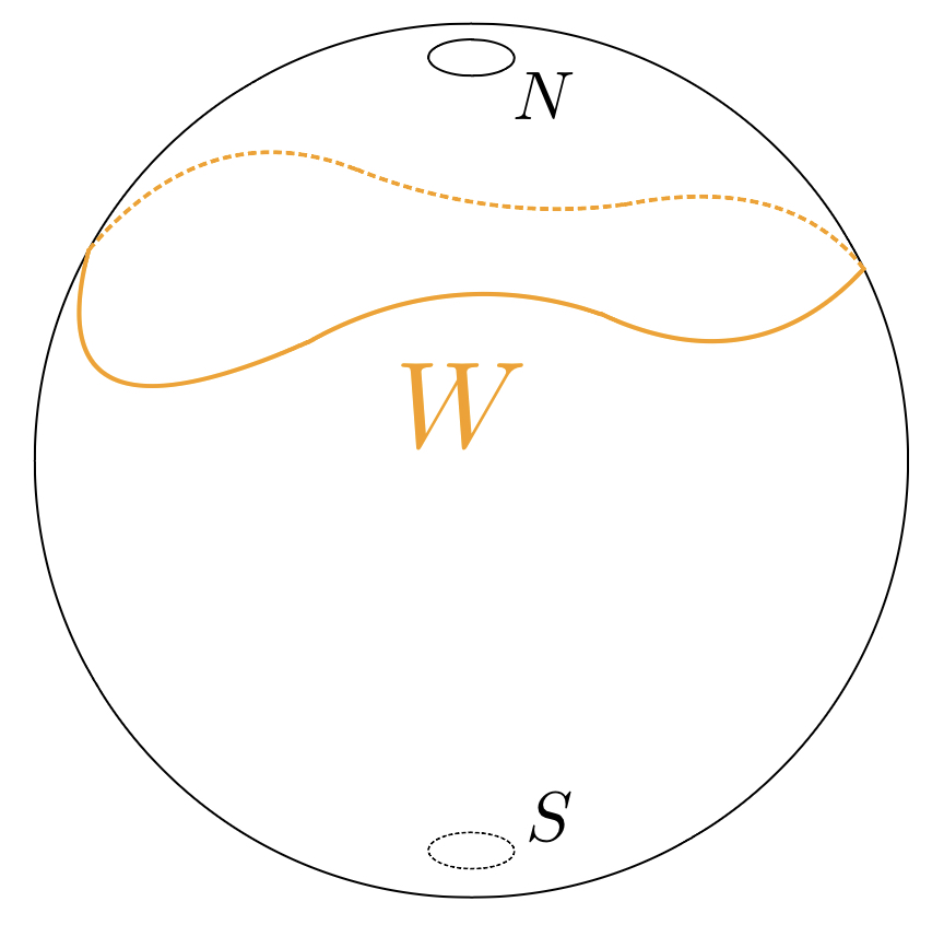
Figure 5: 1/8-BPS Wilson loop on $S^{2}$ wrapping around the surface operator.

Since we are interested in the normalized correlator, we start with the computation of the expectation value of the surface operator. In the heat kernel lattice formulation, we cover the Riemann surface with arbitrary polygons and assign each link $l$ with a group variable $U_{l}\in G$ which is a parallel transport of the gauge connection along $l$. The partition function in this formulation reduces to finite integrals over $U_{l}$ with appropriately normalized Haar measure and for the integrand, we assign for each plaquette $p$ a factor of

$$Z_{p}(U_{p},{\mathcal{A}}_{p})=\sum_{{\mathcal{R}}\in\text{Irrep}\,G}d_{\mathcal{R}}\chi_{\mathcal{R}}(U_{p})e^{-{1\over 4}g^{2}_{2d}{\mathcal{A}}_{p}C_{2}({\mathcal{R}})},$$ (4.80)

where ${\mathcal{A}}_{p}$ is an area of plaquette $p$.

In our case, we have punctures at the North and South poles with holonomies, therefore we can decompose the sphere into a single polygon according to figure 6. One subtle difference compared to the ordinary $2d$ Yang-Mills is that since the structure group at the boundary is $T_{G}$ (see discussion below (4.45)), we would expect an additional overall factor related to the difference of the gauge group. We leave the precise determination of this factor for the future work, and merely call it as $V_{\alpha,\beta}$ since it will generically depends on the holonomies at the boundary. In any case, it drops out in normalized correlators. This way we get

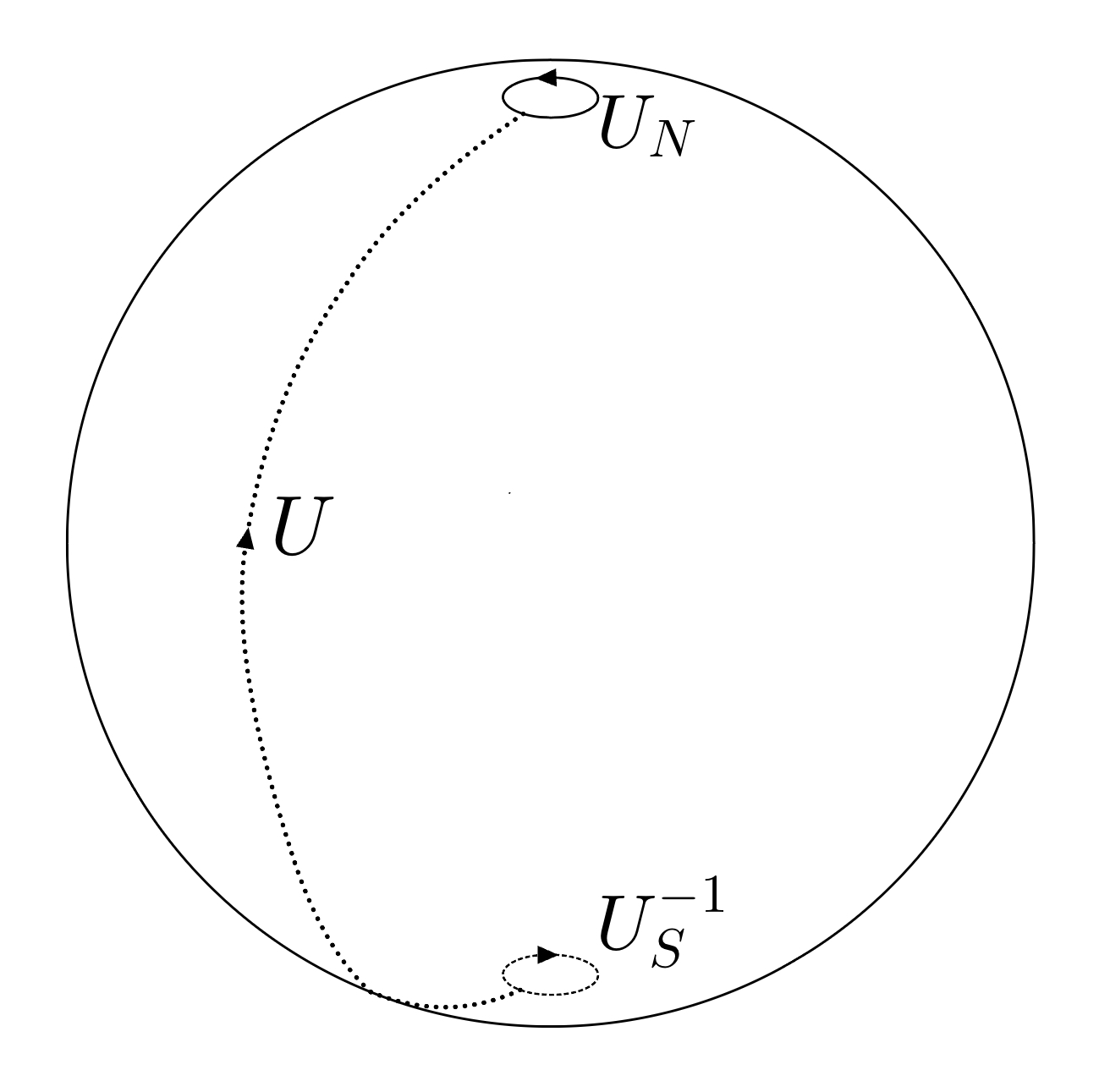
Figure 6: Covering of punctured sphere by a polygon.

$$Z_{\Sigma}^{YM_{2}}=V_{\alpha,\beta}\,e^{8\pi^{2}\beta^{2}\over g_{2d}^{2}{\mathcal{A}}}\sum_{{\mathcal{R}}\in\text{Irrep}\,G}\chi_{{\mathcal{R}}}(U_{N})\chi_{{\mathcal{R}}}(U_{S}^{-1})e^{-{1\over 4}g^{2}_{2d}{\mathcal{A}}C_{2}({\mathcal{R}})},$$ (4.81)

where ${\mathcal{A}}=4\pi$ is an area of $S^{2}$, $U_{N,S}$ are holonomies at north and south poles in (4.45), and the sum is over irreducible representations of $G=U(N)$, where in our case, it is labeled by N-tuples of integers ${\mathcal{R}}=(\lambda_{1},\dots,\lambda_{N})$ which satisfy $\infty>\lambda_{1}\geq\lambda_{2}\geq\dots\geq\lambda_{N}\geq-\infty$. The quadratic Casimir is given by

$$C_{2}({\mathcal{R}})=\sum_{i=1}^{N}\lambda_{i}^{2}+(N+1-2i)\lambda_{i},$$ (4.82)

which can be simplified in terms of $l_{i}=\lambda_{i}+N-i$ so that $\{l_{i}\}$ are strictly decreasing $\infty>l_{1}>l_{2}>\dots>l_{N}>-\infty$ as

$$C_{2}({\mathcal{R}}) =-{1\over 12}N(N^{2}-1)+\sum_{i=1}^{N}\left(l_{i}-{N-1\over 2}\right)^{2}.$$ (4.83)

Now $U_{N,S}\in G_{\mathbb{C}}\simeq GL(N,\mathbb{C})$, and since any $U(N)$ representation can be naturally extended to $GL(N,\mathbb{C})$, we naturally take $\chi_{{\mathcal{R}}}$ to be a character of $GL(N,\mathbb{C})$. The explicit representation of the character for $e^{y}\in T_{\mathbb{C}}=(\mathbb{C}^{*})^{N}$ is given by

$$\chi_{{\mathcal{R}}}(e^{y})={\det e^{y_{a}l_{b}}\over\det e^{y_{a}(N-b)}},$$ (4.84)

where $a$ and $b$ denote row and column of matrices with $y=\text{diag}(y_{1},\dots,y_{N})$. Note that in our case $y=\pm\alpha+i\beta$, and hence the character formula (4.84) only makes sense for $\mathbb{L}=U(1)^{N}$ and becomes singular for generic $\mathbb{L}=\prod_{j=1}^{M}U(N_{j})$. In this case, we apply L’Hôpital’s rule to obtain the character formula for singular element in $GL(N,\mathbb{C})$ as

$$\chi_{{\mathcal{R}}}(e^{y})={1\over D(y)\prod_{j=1}^{M}\prod_{s=1}^{N_{j}}s!}\sum_{w\in S_{N}}{\varepsilon}(w)e^{\sum_{a=1}^{N}y_{w(a)}l_{a}}\prod_{j=1}^{M}\Delta(l_{w^{-1}(1+\sum_{k=1}^{j-1}N_{k})},\dots,l_{w^{-1}(N_{j})})$$ (4.85)

$$D(y)\equiv e^{\sum_{j=1}^{M}{1\over 2}N_{j}(N_{j}-1)y_{[j]}}\prod\limits_{\begin{subarray}{c}a<b=1\\ [a]\neq[b]\end{subarray}}^{N}(e^{y_{a}}-e^{y_{b}}),\quad\Delta(l_{1},\dots,l_{N})\equiv\prod_{a<b=1}^{N}(l_{a}-l_{b}),$$

where we ordered $y$ such that $y=\text{diag}(y_{1},\dots,y_{N})=\text{diag}(\overbrace{y_{[1]},\dots,y_{[1]}}^{N_{1}},\dots,\overbrace{y_{[M]},\dots y_{[M]}}^{N_{M}})$ so that $y_{a}$ belongs to $[a]$-th block.

To extract the zero-instanton sector of $Z_{\Sigma}^{YM_{2}}$ (4.81) we use the Poisson summation formula [84, 83],

$$\sum_{-l_{i}=-\infty}^{\infty}f(l_{1},\dots,l_{N}) =\sum_{m_{i}=-\infty}^{\infty}\int_{-\infty}^{\infty}dz_{1}\dots dz_{N}\,e^{2\pi i\sum_{i=1}^{N}m_{i}z_{i}}f(z_{1},\dots,z_{N})$$ (4.86)

$$\equiv\sum_{m_{i}=-\infty}^{\infty}F(m_{1},\dots,m_{N}),$$

which identifies the zero-instanton sector as $m_{1}=\dots=m_{N}=0$ contribution. This way, we get

$$Z_{\Sigma}^{YM_{2}}|_{0-inst}= V_{\alpha,\beta}e^{8\pi^{2}\beta^{2}\over g_{2d}^{2}{\mathcal{A}}}c(\{N_{i}\},g,\alpha,\beta)$$ (4.87)

$$\left(\sum_{w\in S_{N}}{\varepsilon}(w)e^{2\pi(\alpha+i\beta)_{w(a)}z_{a}}\prod_{j=1}^{M}\Delta(z_{w^{-1}(1+\sum_{i=1}^{j-1}N_{i})},\dots,z_{w^{-1}(N_{j})})\right)$$

$$\left(\sum_{\widetilde{w}\in S_{N}}{\varepsilon}(\widetilde{w})e^{2\pi(-\alpha+i\beta)_{\widetilde{w}(a)}z_{a}}\prod_{j=1}^{M}\Delta(z_{\widetilde{w}^{-1}(1+\sum_{i=1}^{j-1}N_{i})},\dots,z_{\widetilde{w}^{-1}(N_{j})})\right)$$

$$\exp\left(-{1\over 4}g^{2}_{2d}\mathcal{A}\sum_{i=1}^{N}(z_{i}-{N-1\over 2})^{2}\right),$$

where

$$c_{W}(\{N_{i}\},g_{2d},\alpha,\beta)={e^{{1\over 48}g^{2}_{2d}\mathcal{A}N(N^{2}-1)}\over N!|D(\alpha+i\beta)|^{2}\prod_{j=1}^{M}\prod_{s=1}^{N_{j}}(s!)^{2}}.$$ (4.88)

The sums over $w$ and $\widetilde{w}$ reflect the freedom of independent Weyl transformation on the holonomies around the North and South poles in the standard $2d$ Yang-Mills setup. This is natural, because the standard $2d$ Yang-Mills path integral localizes to instantons [62] and the independent Weyl transformations on the North and South poles generate different saddle points (c.f. [85]).

However, our holonomies at the Sorth and South poles are fixed and hence cannot have an independent Weyl transformation. Therefore, the true $2d$ sector describing $4d$ sector is described by the pair $(w,\widetilde{w})\in W\times W$ satisfying $\pm\alpha+i\beta=w\cdot(\pm\alpha+i\beta)=\widetilde{w}\cdot(\pm\alpha+i\beta)$. There are $(\prod_{j=1}^{M}N_{j}!)^{2}$ such pairs. The remaining integration over $\{z_{a}\}$ is purely Gaussian and we get $4d$ vev of the surface operator from the $B^{3}\times S^{1}$ localization as

$$\langle{\mathcal{O}}_{\Sigma}\rangle_{B^{3}\times S^{1}}=V_{\alpha,\beta}\left(\prod_{j=1}^{M}N_{j}!\right)^{2}c_{W}(\{N_{i}\},g_{2d},\alpha,\beta)e^{2\pi i(N-1)\sum_{i}\beta_{i}}\left(\prod_{p=1}^{M}G_{p}\right),$$ (4.89)

where

$$G_{p} =\int\left(\prod_{a=1}^{N_{p}}dx_{a}\right)\Delta(x_{1},\dots,x_{N_{p}})^{2}e^{-{1\over 4}g_{2d}^{2}{\mathcal{A}}\sum_{a}x_{a}^{2}}$$ (4.90)

$$=\left({g_{2d}^{2}{\mathcal{A}}/2}\right)^{-N_{p}^{2}/2}(2\pi)^{N_{p}/2}\left(\prod_{n=1}^{N_{p}}n!\right).$$

Therefore, we see that (4.89) is also a Gaussian matrix model with a one-loop measure $\Delta_{\mathbb{L}}$ as in (3.32).

Therefore in terms of $4d$ gauge coupling $g^{2}$, we finally get

$$\langle{\mathcal{O}}_{\Sigma}\rangle_{B^{3}\times S^{1}}={V_{\alpha,\beta}e^{2\pi i(N-1)\sum_{i=1}^{N}\beta_{i}}\over|D(\alpha+i\beta)|^{2}}{\left(\prod_{j=1}^{M}N_{j}!\right)(2\pi)^{N/2}(-g^{2})^{-\text{dim}(\mathbb{L})/2}e^{-{1\over 24}g^{2}N(N^{2}-1)}\over N!\prod_{j=1}^{M}\prod_{s=1}^{N_{j}-1}s!},$$ (4.91)

where we note that the exponential term $e^{-{1\over 24}g^{2}N(N^{2}-1)}=e^{{1\over 48}g_{2d}^{2}{\mathcal{A}}N(N^{2}-1)}$ can be removed by a local counterterm in $2d$ proportional to $\int_{S^{2}}\sqrt{g_{S^{2}}}$, and the denominator $\prod_{j=1}^{M}\prod_{s=1}^{N_{j}-1}s!$ is proportional to the $\text{vol}(\mathbb{L})$. However, there are still some qualitative differences compared to the $4d/2d$ localization computation of the vev of the $S^{2}$ surface operator in $S^{4}$ (3.35) and we comment on them.

First, we see that there is no radius dependence of the vev. This is consistent with our claim of the absence of the surface Weyl anomaly on $B^{3}\times S^{1}$ discussed at the end of section 4.3.

Secondly, a difference between overall powers of $g^{2}$, which originated from the Gaussian matrix model with exponent proportional to $g^{2}$ compared to $1/g^{2}$ in section 3.1. Since this cannot be compensated by any local counterterm on $S^{2}$, it is natural to guess that the one-loop determinant from the $B^{3}\times S^{1}$ localization would produce such a factor difference (the localization determinant was not computed in [56]). This factor is also needed for the vacuum partition function (c.f. [58]).

Thirdly, there are purely $\alpha,\beta$ dependent factors appearing in the first factor in (4.91). These factors have to be canceled since we expect the vev of the surface operators on $B^{3}\times S^{1}$ are trivial as the planar surface operators on $\mathbb{R}^{4}$. One observation is that

$$|D(\alpha+i\beta)|^{2}=e^{\sum_{j=1}^{M}iN_{j}(N_{j}-1)\beta_{[j]}}\prod\limits_{\begin{subarray}{c}a<b=1\\ [a]\neq[b]\end{subarray}}^{N}|e^{(\alpha+i\beta)_{a}}-e^{(\alpha+i\beta)_{b}}|^{2}\,,$$ (4.92)

where the 2nd product factor is proportional to the (analytically continued) volume of the conjugacy class of $e^{\alpha+i\beta}$ (or equivalently $e^{-\alpha+i\beta}$) in $G=U(N)$. Therefore we anticipate that this volume factor is canceled by $V_{\alpha,\beta}$. On the other hand, using $\langle\bm{F}\rangle=i\beta\text{vol}_{S^{2}}$, we might expect the $e^{\beta_{j}}$ factors will be canceled by the ABJ anomaly of massless fermions at the level of constrained $2d$ YM (c.f. (4.29)), which is responsible for the restriction to the perturbative sector.

In the end, it turns out that these subtle factors will similarly appear in the correlator $\langle W_{F}{\mathcal{O}}_{\Sigma}\rangle$, and therefore the above subtleties are inconsequential when we compute the normalized correlator. Therefore we proceed and leave a careful determination of the vev on $B^{3}\times S^{1}$ from this localization to the future. The computation in a different localization was already presented in section 3.1.

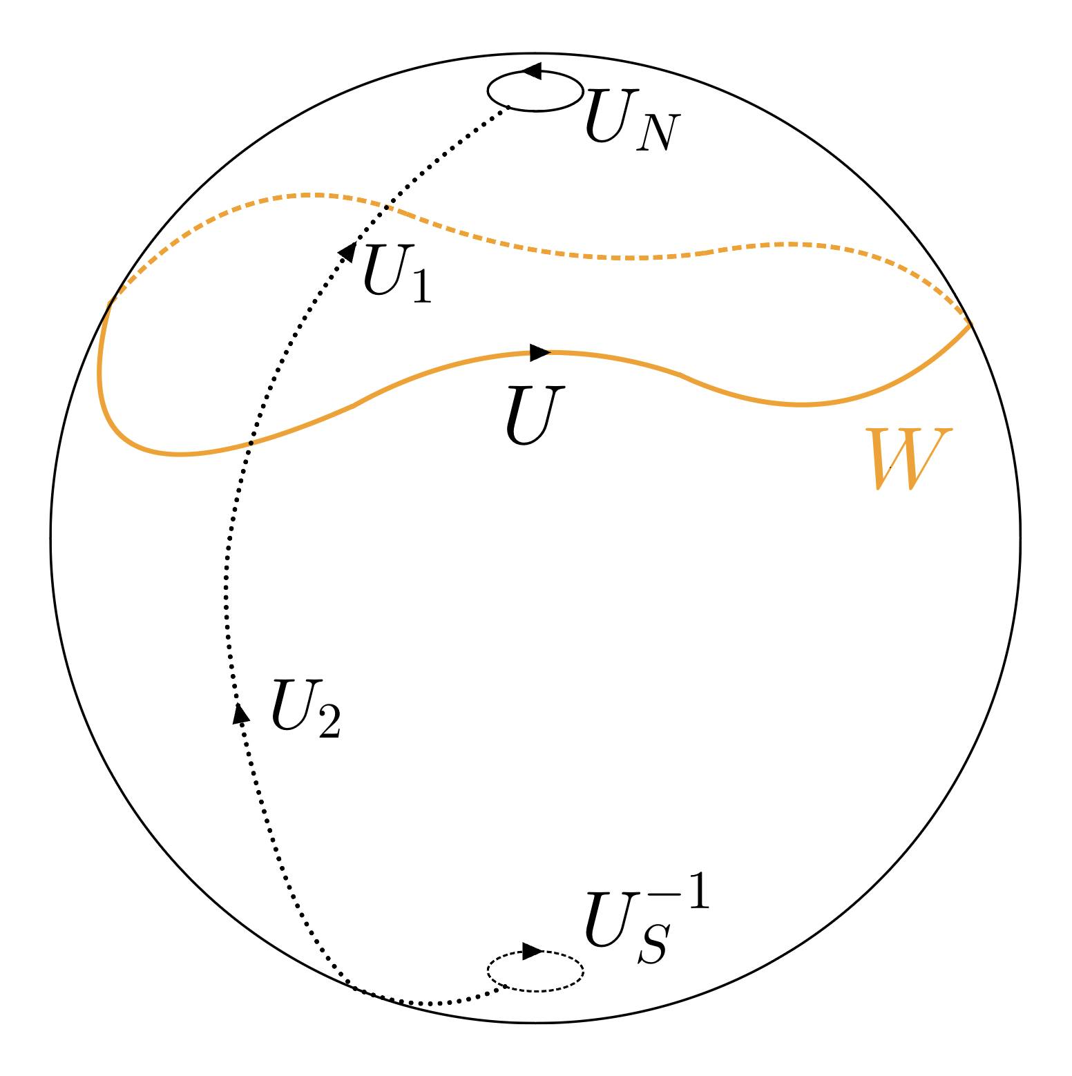
Figure 7: Covering of punctured sphere with Wilson loops by polygons.

Next, we compute the correlation function of the fundamental Wilson loop wrapping non-trivially the North and the South poles as in figure 5. Using the lattice decomposition as in figure 7, we get

$$\langle W_{F}{\mathcal{O}}_{\Sigma}\rangle^{YM_{2}}= V_{\alpha,\beta}\,e^{8\pi^{2}\beta^{2}\over g_{2d}^{2}{\mathcal{A}}}\sum_{{\mathcal{R}}_{1},{\mathcal{R}}_{2}}\chi_{{\mathcal{R}}_{1}}(U_{N})\chi_{{\mathcal{R}}_{2}}(U_{S}^{-1})e^{-{1\over 2}g_{2d}^{2}[{\mathcal{A}}_{1}C_{2}({\mathcal{R}}_{1})+{\mathcal{A}}_{2}C_{2}({\mathcal{R}}_{2})]}$$ (4.93)

$$\int dg\chi_{F}(g)\chi_{R_{1}}(g^{-1})\chi_{R_{2}}(g).$$

The fundamental representation is given by $F=(1,0,\dots,0)$. Then we can similarly extract the 0-instanton sector as

$$\langle W_{F}{\mathcal{O}}_{\Sigma}\rangle^{YM_{2}}|_{0-inst}= V_{\alpha,\beta}\,e^{8\pi^{2}\beta^{2}\over g_{2d}^{2}{\mathcal{A}}}c_{W}(\{N_{i}\},g_{2d},\alpha,\beta)$$ (4.94)

$$\int dz_{a}\sum_{k=1}^{N}\left(\sum_{w\in S_{N}}{\varepsilon}(w)e^{2\pi(\alpha+i\beta)_{w(a)}z_{a}}\prod_{j=1}^{m}\Delta(z_{w^{-1}(1+\sum_{i=1}^{j-1}N_{i})},\dots,z_{w^{-1}(N_{j})})\right)$$

$$\left(\sum_{w\in S_{N}}{\varepsilon}(w)e^{2\pi(-\alpha+i\beta)_{w(a)}\widetilde{z}_{a}}\prod_{j=1}^{m}\Delta(\widetilde{z}_{w^{-1}(1+\sum_{i=1}^{j-1}N_{i})},\dots,\widetilde{z}_{w^{-1}(N_{j})})\right)$$

$$\exp\left(-{1\over 4}g^{2}_{2d}\mathcal{A}_{1}\sum_{i=1}^{N}(z_{i}-{N-1\over 2})^{2}-{1\over 4}g^{2}_{2d}\mathcal{A}_{2}\sum_{i=1}^{N}(z_{i}-\delta_{k,i}-{N-1\over 2})^{2}\right).$$

Again, the true $0$-instanton sector is described by further extracting only $(w,\widetilde{w})\in W\times W$ satisfying $\pm\alpha+i\beta=w\cdot(\pm\alpha+i\beta)=\widetilde{w}\cdot(\pm\alpha+i\beta)$. Therefore we get the Wilson loop correlator in $4d$ on $B^{3}\times S^{1}$ as

$$\langle W_{F}{\mathcal{O}}_{\Sigma}\rangle_{B^{3}\times S^{1}}= V_{\alpha,\beta}\left(\prod_{j=1}^{m}N_{j}!\right)^{2}c_{W}(\{N_{i}\},g_{2d},\alpha,\beta)e^{2\pi i(N-1)\sum_{i}\beta_{i}}e^{-{1\over 4}g_{2d}^{2}{\mathcal{A}}_{2}}e^{{g_{2d}^{2}{\mathcal{A}}_{2}^{2}\over 2{\mathcal{A}}}}$$ (4.95)

$$\sum_{l=1}^{m}N_{l}e^{2\pi(\alpha_{l}-i\beta_{l}{{\mathcal{A}}_{1}-{\mathcal{A}}_{2}\over{\mathcal{A}}})}F_{l}\prod_{\begin{subarray}{c}p=1,\dots,m\\ p\neq l\end{subarray}}G_{p},$$

where $G_{p}$ is defined in (4.90) and $F_{l}$ is given by

$$F_{l} =\int\left(\prod_{a=1}^{N_{l}}dx_{a}\right)\Delta(x_{a}-\delta_{a,1}{\mathcal{A}}_{1}/{\mathcal{A}})\Delta(x_{a}+\delta_{a,1}{\mathcal{A}}_{2}/{\mathcal{A}})e^{-{1\over 4}g_{2d}^{2}{\mathcal{A}}\sum_{a}x_{a}^{2}}$$ (4.96)

$$=(g_{2d}^{2}{\mathcal{A}}/2)^{-N_{l}^{2}/2}(N_{l}-1)!(2\pi)^{N_{l}/2}\left(\prod_{n=1}^{N_{l}-1}n!\right)L^{1}_{N_{l}-1}\left(g_{2d}^{2}{{\mathcal{A}}_{1}{\mathcal{A}}_{2}\over 2{\mathcal{A}}}\right).$$

As a consequence, we reach at the exact normalized correlator

$${\langle W_{F}{\mathcal{O}}_{\Sigma}\rangle_{B^{3}\times S^{1}}\over\langle{\mathcal{O}}_{\Sigma}\rangle_{B^{3}\times S^{1}}}=\sum_{l=1}^{m}{N_{l}\over N}e^{2\pi(\alpha_{l}-i\beta_{l}{{\mathcal{A}}_{1}-{\mathcal{A}}_{2}\over{\mathcal{A}}})}{1\over N_{l}}L_{N_{l}-1}^{1}\left(g_{2d}^{2}{{\mathcal{A}}_{1}{\mathcal{A}}_{2}\over 2{\mathcal{A}}}\right)e^{-g_{2d}^{2}{{\mathcal{A}}_{1}{\mathcal{A}}_{2}\over 4{\mathcal{A}}}}.$$ (4.97)

To compare with the supergravity result in [1], we first take the large $N$ limit $N_{l}\gg 1$ and $\lambda=g^{2}N$ fixed, which gives

$${\langle W_{F}{\mathcal{O}}_{\Sigma}\rangle_{B^{3}\times S^{1}}\over\langle{\mathcal{O}}_{\Sigma}\rangle_{B^{3}\times S^{1}}}\Bigg{|}_{\text{large $N$}} \simeq\sum_{l=1}^{m}{N_{l}\over N}e^{2\pi(\alpha_{l}-i\beta_{l}{{\mathcal{A}}_{1}-{\mathcal{A}}_{2}\over{\mathcal{A}}})}{J_{1}\left(2\sqrt{N_{l}g^{2}_{2d}{{\mathcal{A}}_{1}{\mathcal{A}}_{2}\over 2{\mathcal{A}}}}\right)\over\sqrt{N_{l}g^{2}_{2d}{{\mathcal{A}}_{1}{\mathcal{A}}_{2}\over 2{\mathcal{A}}}}}$$ (4.98)

$$=\sum_{l=1}^{m}{N_{l}\over N}e^{2\pi(\alpha_{l}-i\beta_{l}{{\mathcal{A}}_{1}-{\mathcal{A}}_{2}\over{\mathcal{A}}})}{2I_{1}\left(\sqrt{{\lambda N_{l}\over N}{4{\mathcal{A}}_{1}{\mathcal{A}}_{2}\over{\mathcal{A}}^{2}}}\right)\over\sqrt{{\lambda N_{l}\over N}{4{\mathcal{A}}_{1}{\mathcal{A}}_{2}\over{\mathcal{A}}^{2}}}}.$$

If we further take the strong coupling limit $\lambda\rightarrow\infty$, we get

$${\langle W_{F}{\mathcal{O}}_{\Sigma}\rangle_{B^{3}\times S^{1}}\over\langle{\mathcal{O}}_{\Sigma}\rangle_{B^{3}\times S^{1}}}\Bigg{|}_{\text{strong coupling}}\simeq\sum_{l=1}^{m}{N_{l}\over N}e^{2\pi(\alpha_{l}-i\beta_{l}{{\mathcal{A}}_{1}-{\mathcal{A}}_{2}\over{\mathcal{A}}})}\sqrt{2\over\pi}{\exp\left(\sqrt{{\lambda N_{l}\over N}{4{\mathcal{A}}_{1}{\mathcal{A}}_{2}\over{\mathcal{A}}^{2}}}\right)\over\left({\lambda N_{l}\over N}{4{\mathcal{A}}_{1}{\mathcal{A}}_{2}\over{\mathcal{A}}^{2}}\right)^{3/4}}.$$ (4.99)

This is beautifully consistent with the supergravity result [1] upon converting parameters accordingly, where the computation was restricted to the 1/4 BPS Wilson loop so that it has a circular geometry with a fixed latitude on $S^{2}$.

In Appendix F we analyze the effective propagator of the circular BPS Wilson loop holonomy in the surface operator background (using background field method and Feynman gauge) and show that it is constant and non-zero in the Levi blocks. This implies that summing over the rainbow diagrams in the surface operator background exactly reproduces (4.97) (c.f.[86, 87]).

Appendix A Geometry of $B^{3}\times S^{1}$

The relation between $\mathbb{R}^{4}$ and $B^{3}\times S^{1}$ can be understood as consecutive Weyl transformations, first from $\mathbb{R}^{4}$ to $S^{4}$ and then from $S^{4}$ to $B^{3}\times S^{1}$. From $\mathbb{R}^{4}$ coordinates $\{x_{i}\}$ with a standard Euclidean metric $ds^{2}=dx_{i}^{2}$, we have a standard stereographic projection to $S^{4}$ of radius $R/2$

$$g_{\mu\nu}(S^{4})=e^{2w_{1}}g_{\mu\nu}(\mathbb{R}^{4}),\quad e^{w_{1}}=\left(1+{x^{2}\over R^{2}}\right)^{-1}.$$ (A.1)

Next we write $S^{4}$ coordinate in terms of the embeeding coordinates $\{X_{A}\}$ with $A=1,\dots,5$ satisfying $\sum_{A}X_{A}^{2}=r^{2}$. We divide the embedding coordinates into $(X_{1},X_{5})$ and $(X_{2},X_{3},X_{4})$ such that $SO(2)\times SO(3)$ isometry is explicit. Then relation to the $B^{3}\times S^{1}$ coordinates is given by

$$X_{1}+iX_{5}=r\left(1-{\widetilde{x}^{2}\over R^{2}}\right)\left(1+{\widetilde{x}^{2}\over R^{2}}\right)^{-1}e^{i\tau}$$ (A.2)

$$X_{i}={\widetilde{x}_{i}}\left(1+{\widetilde{x}^{2}\over R^{2}}\right)^{-1},\quad i=2,3,4,$$

together with the Weyl transformation

$$g_{\mu\nu}(B^{3}\times S^{1})=e^{2w_{2}}g_{\mu\nu}(S^{4}),\quad e^{w_{2}}=\left(1+{\widetilde{x}^{2}\over R^{2}}\right).$$ (A.3)

Therefore the total Weyl transformation from $\mathbb{R}^{4}$ to $B^{3}\times S^{1}$ is given by

$$g_{\mu\nu}(B^{3}\times S^{1})=e^{2w}g_{\mu\nu}(\mathbb{R}^{4}),\quad e^{w}={1+\widetilde{x}^{2}+(1-\widetilde{x}^{2})\cos\tau\over 2},$$ (A.4)

which gives the metric (4.1)

Appendix B $\mathcal{N}=4$ Super Yang-Mills Theory

The Euclidean ${\mathcal{N}}=4$ SYM on Riemannian four-manifold $(M,h_{\mu\nu})$ is given by

$$S=\int_{M}\mathcal{L}_{bulk}\sqrt{h}d^{4}x=\int{1\over g^{2}}\left({1\over 2}F_{MN}F^{MN}-\lambda\Gamma^{M}D_{M}\lambda+{\bm{R}\over 6}\phi^{I}\phi_{I}\right)\sqrt{h}\,d^{4}x,$$ (B.1)

where $\bm{R}$ is the scalar curvature and we are using 10d notation following [46] such that $M=1,2,\dots,9,0$ and $A_{\mu}$ with $\mu=1,\dots,4$ is a four-dimensional gauge field, $A_{I}=\phi_{I}$ with $I=5,\dots,9,0$ denotes 6 adjoint scalars, and $\lambda\in S^{+}$ is a dimensionally reduced $Spin(10)$ Weyl Spinor with positive chirality. Also, see footnote 27 for our convention for the bilinear form on $\mathfrak{g}$.

Following [46], our choice of basis $\gamma_{M}\in\{\gamma_{1},\dots,\gamma_{9},\gamma_{0}\}$ of the Clifford algebra $Cl(10)$ is such that

$$\{\gamma^{M},\gamma^{N}\}=2\delta^{MN}.$$ (B.2)

In the chiral representation, we have

$$\gamma^{M}=\begin{pmatrix}0&\widetilde{\Gamma}^{M}\\ \Gamma^{M}&0\end{pmatrix},$$ (B.3)

where $\widetilde{\Gamma}^{M}=(\Gamma^{1},\dots,\Gamma^{9},-\Gamma^{0})$, and we choose them explicitly as

$$\Gamma_{1}=\begin{pmatrix}1_{8\times 8}&0\\ 0&i1_{8\times 8}\end{pmatrix},\quad\Gamma_{M=2,\dots,9}=\begin{pmatrix}0&E_{M}^{T}\\ E_{M}&0\end{pmatrix},{} \Gamma_{0}=\begin{pmatrix}i1_{8\times 8}&0\\ 0&i1_{8\times 8}\end{pmatrix},$$ (B.4)

where $E_{M=2,\dots,9}$ are matrices representing the left multiplication of the octonion and we take $E_{9}$ to be identity such that $E_{9}=1_{8\times 8}$. Explicitly, we have $(E_{i})^{k}_{j}=c^{k}_{ij}$ where $c^{k}_{ij}$ is the structure constant of the octonion algebra $e_{i}\cdot e_{j}=c_{ij}^{k}e_{k}$. We choose a cylic quaternionic triple multiplication table as $(234),(256),(357),(458),(836),(647),(728)$ such that $e_{9}$ is an identity and $e_{2}e_{3}=e_{4}$, etc.

The chirality matrix is given by

$$\gamma_{c}=-i\gamma^{1}\dots\gamma^{9}\gamma^{0},$$ (B.5)

under which, 32 components spinors in Dirac representation $\mathcal{S}$ decomposes in to two 16 components Weyl spinors of positive and negtaive chirality as $\mathcal{S}\simeq\mathcal{S}^{+}\oplus\mathcal{S}^{-}$.

Given the conformal-Killing spinor $\epsilon$ on $M$ whose defining equation is

$$\nabla_{\mu}\epsilon=\widetilde{\Gamma}_{\mu}\widetilde{\epsilon},$$ (B.6)

there is an superconformal symmetry given by

$$\delta_{\epsilon}A_{M}=\epsilon\Gamma_{M}\lambda,\quad\delta_{\epsilon}\lambda={1\over 2}F_{MN}\Gamma^{MN}\epsilon+{1\over 2}\Gamma_{\mu A}\phi^{A}\nabla^{\mu}\epsilon.$$ (B.7)

Note that superconformal algebra is only closed on-shell (for off-shell realization see [60, 46].)

The variation of the action under $\delta_{\epsilon}$ is given by

$$\delta_{\epsilon}S={1\over g^{2}}\int_{M}\nabla_{\mu}\left(\epsilon\Gamma_{M}\lambda F^{\mu M}+{1\over 2}F_{MN}\epsilon\Gamma^{\mu MN}\lambda+2\phi_{I}\widetilde{\epsilon}\Gamma^{I\mu}\lambda\right)\sqrt{h}\,d^{4}x.$$ (B.8)

On the other hand, the Euler-Lagrange variation is given by

$$\delta S={1\over g^{2}}\int_{M}\left[\nabla_{\mu}\left(2\delta A_{M}F^{\mu M}-\lambda\Gamma^{\mu}\delta\lambda\right)+\delta A_{M}\cdot(eom)_{A_{M}}+\lambda\cdot(eom)_{\lambda}\right]\sqrt{h}\,d^{4}x,$$ (B.9)

where $eom_{X}$ denotes the Euler-Lagrange equations of motion come from the variation $\delta_{X}$.

Appendix C $\langle{\cal O}_{S^{2}}\rangle_{S^{4}}$ From Disorder Definition

In this Appendix we compute the vev of a surface operator wrapping a maximal $S^{2}$ in $S^{4}$ using the disorder definition of ${\cal O}_{\Sigma}$ given in section 2. This yields the same answer (3.9) found in section 3 using the coupled $4d/2d$ system.

We choose the localizing supercharge used by Pestun in [46] to compute the $S^{4}$ partition function and Wilson loops of $4d$ ${\cal N}=2$ SCFTs. In [57] the computation of the ’t Hooft loop disorder operator was performed, and here we compute $\langle{\cal O}_{S^{2}}\rangle_{S^{4}}$.

The first step is to determine the space of supersymmetric saddle points in the presence of the singularity produced by the surface operator ${\cal O}_{S^{2}}$. The saddle point is the field configuration in Pestun’s original computation with the additional surface operator background turned on [88]. The ${\cal N}=4$ SYM action evaluated on the saddle points yields [88]

$$S=-{8\pi^{2}\over g^{2}}\left(a^{2}+2ia\alpha\right)\,.$$ (C.1)

Then there are the perturbative and non-perturbative corrections. The nonperturbative corrections are captured by the the ramified instanton partition function at the North pole and the ramified anti-instanton partition function at the South pole (see e.g. [89] are references within for details on ramified instanton partition functions).

If we consider ${\cal N}=4$ SYM with the insertion of ${\cal O}_{S^{2}}$ then the expectation is that $Z_{\text{ramified}}$=1 due to fermion zero modes. These are lifted for ${\cal N}=2$ theories, including for ${\cal N}=2^{*}$ (for a related discussion in the absence of surface operators see [54]).

There remains the one-loop contribution around the localization locus. This factorizes into the product from the North pole and the South pole. Therefore, $\langle{\cal O}_{S^{2}}\rangle_{S^{4}}$ in ${\cal N}=4$ SYM is given by

$$\langle{\cal O}_{S^{2}}\rangle_{S^{4}}=\int dae^{-{8\pi^{2}\over g^{2}}\left(a^{2}+2ia\alpha\right)}Z_{\text{1-loop}}(a(N))\overline{Z}_{\text{1-loop}}(a(S))\,.$$ (C.2)

$a(N)$ and $a(S)$ are the values of the scalar field in ${\cal N}=2$ vector multiplet in the localizing locus in the presence of the background produced by ${\cal O}_{S^{2}}$. They are given by [88]

$$a(N)=a(S)=a+i(\alpha-\lceil\alpha\rceil)\,,$$ (C.3)

where $\lceil\alpha\rceil$ is the ceiling function. This combination ensures periodicity of the path integral under $\alpha\rightarrow\alpha+1$. Physically, it encapsulates that in the presence of surface operator there are normalizable, singular modes that contribute to the one-loop determinant. The importance of these singular modes has been found in other dimensions for vortex loops [90, 91, 92, 78] in $3d$ and vortex operators in $2d$ [93, 85].

Both in the classical action and one-loop determinants we can shift the integration variable

$$a\rightarrow a+i\alpha$$ (C.4)

and then the one-loop determinant in ${\cal N}=4$ SYM in presence of ${\cal O}_{S^{2}}$ are (see e.g. [46, 57])

$$Z_{\text{1-loop}}=\prod_{\bm{\alpha}}{{\Upsilon(i\bm{\alpha}\cdot a+\lceil\bm{\alpha}\cdot\alpha\rceil)}\over\Upsilon(1+i\bm{\alpha}\cdot a+\lfloor\bm{\alpha}\cdot\alpha\rfloor)}\,,$$ (C.5)

where $\bm{\alpha}$ are the roots of the Lie algebra of $G$, the gauge group of ${\cal}=4$ SYM. $\lfloor\alpha\rfloor$ is the floor function.

The formula can be greatly simplified by separating the product over roots into those that have $\bm{\alpha}\cdot\alpha>0,\bm{\alpha}\cdot\alpha<0$ and $\bm{\alpha}\cdot\alpha=0$. Remarkably, only the roots with $\bm{\alpha}\cdot\alpha=0$ contribute, the rest cancel between the vector multiplet and hypermultiplet, and yield

$$Z_{\text{1-loop}}=\prod_{\bm{\alpha}\cdot\alpha=0}{\Upsilon(i\bm{\alpha}\cdot a)\over\Upsilon(i\bm{\alpha}\cdot a+1)}=\prod_{\bm{\alpha}\cdot\alpha=0,\bm{\alpha}}{1\over\gamma(i\bm{\alpha}\cdot\alpha)\gamma(-i\bm{\alpha}\cdot\alpha)}=\Delta_{\mathbb{L}}(a)\,,$$ (C.6)

where we have used the shift properties of $\Upsilon(x+1)=\gamma(x)\Upsilon(x)$.

Putting everything together, and reintroducing the sphere radius, we recover what we found from the computation in section 3 using the $4d/2d$ definition

$$\langle{\cal O}_{S^{2}}\rangle_{S^{4}}=\int da\,\Delta_{\mathbb{L}}(a)e^{-{8\pi^{2}\over g^{2}}a^{2}}={r}^{-\text{dim}\,\mathbb{L}}\left({g^{2}\over 4\pi}\right)^{\text{dim}\,\mathbb{L}/2}e^{-8\pi^{2}\alpha^{2}/g^{2}}\,.$$ (C.7)

Appendix D Supersymmetric Boundary Conditions and Boundary Term of Surface Operator in $\mathcal{N}=4$ Super Yang-Mills Theory

D.1.  Planar Surface Operator in $\mathbb{R}^{4}$

In this section, we determine the supersymmetric boundary conditions and boundary terms for the planar surface operator in $\mathbb{R}^{4}$ using the guiding principles explained in section 4.3. We set the planar surface operator’s profile to be $x^{3}=x^{4}=0$. Introducing $\phi_{w}={1\over\sqrt{2}}(\phi^{7}-i\phi^{8})$ and $z=x^{3}+ix^{4}=re^{i\psi}$, the background produced by the surface operator is

$$\phi_{w}={\beta+i\gamma\over\sqrt{2}z},\quad A=\alpha d\psi.$$ (D.1)

The conformal Killing spinors in $\mathbb{R}^{4}$ are given by $\epsilon=\epsilon_{s}+x^{\mu}\widetilde{\Gamma}_{\mu}\epsilon_{c}$, and the surface defect background is preserved by the half of supercharges characterized by the following half-BPS condition

$$\Gamma^{wz}\epsilon_{s}=0,\quad\Gamma^{wz}\epsilon_{c}=0.$$ (D.2)

Next, we regularize the surface operator where we excise the infinitesimal neighborhood around $x_{3}=x_{4}=0$. The most natural cutoff is to have a boundary $\partial M\simeq S^{1}\times\mathbb{R}^{2}$, such that $M:x_{3}^{2}+x_{4}^{2}>\rho^{2}$ has a $\mathbb{R}^{2}\times S^{1}$ with an infinitesimal boundary $\partial M:x_{3}^{2}+x_{4}^{2}=\rho$.

Our task is to find boundary conditions and possible boundary term on $\partial M$ which makes the theory with and has consistent Euler-Lagrange variational principle and manifest supersymmetry.

We first analyze the possible boundary conditions on fermions. Since it is a first-order system, the boundary condition should be a projection that removes half degrees of freedom at the boundary. If we look at B.9, there is the following fermionic part of boundary contribution from the EL principle

$$\int_{\partial M}n_{\mu}\lambda\Gamma^{\mu}\delta\lambda\sqrt{h|_{\partial M}}\,d^{3}x,$$ (D.3)

where $n_{\mu}$ is a (inward) normal vector at the boundary. Note that there is no possible boundary term to compensate it purely algebraically, therefore (D.3) has to be purely vanish by the fermionic boundary condition. The fermionic boundary condition invariant under $SO(4)\times U(1)\times SO(2)_{\parallel}$ of surface operator and makes (D.3) identically vanish is given by

$$\Gamma^{w\overline{z}}\lambda=\Gamma^{\overline{w}z}\lambda=0\quad\text{or}\quad\Gamma^{3478}\lambda=-\lambda\quad\text{(fermionic boundary condition)}.$$ (D.4)

From this, we can determine the bosonic boundary conditions by looking at the superpartner of (D.4). Explicitly, supersymmetry invariance of the boundary condition requires ($P_{+}={1+\Gamma^{3478}\over 2}$)

$$0 =\delta_{\epsilon}{P_{+}\lambda}$$ (D.5)

$$=F_{12}\Gamma^{12}\epsilon+F_{i\widehat{I}}\Gamma^{i\widehat{I}}\epsilon+{1\over 2}F_{\widehat{I}\widehat{J}}\Gamma^{\widehat{I}\widehat{J}}\epsilon+F_{z\overline{z}}\Gamma^{z\overline{z}}\epsilon+F_{w\overline{w}}\Gamma^{w\overline{w}}\epsilon+F_{z\overline{w}}\Gamma^{z\overline{w}}\epsilon+F_{\overline{z}w}\Gamma^{\overline{z}w}\epsilon-2\phi_{\widehat{I}}\widetilde{\Gamma}^{\widehat{I}}\widetilde{\epsilon},$$

where we introduced a label $i,j,\dots=1,2$,  $a,b,\dots=3,4$,  $\widehat{I},\widehat{J},\dots=5,6,9,0$,  $\widehat{A},\widehat{B},\dots=7,8$. Now using (D.2), we see that the bosonic boundary conditions are determined as

$$A_{i}=\phi_{\widehat{I}}=0,\quad D_{z}\phi_{\overline{w}}=D_{\overline{z}}\phi_{w}=F_{z\overline{z}}-{1\over 2}F_{w\overline{w}}=0\quad\text{(bosonic boundary condition)},$$ (D.6)

therefore classically unexcited fields $(A_{i},\phi_{\widehat{I}})$ obey Dirichlet boundary conditions and excited fields $(A_{a},\phi_{\widehat{A}})$ obey Neumann boundary conditions.

Given the boundary conditions, the remaining task is to determine the boundary term. First, we look at the Euler-Lagrange variation. Imposing the boundary conditions on (B.9), we have an on-shell bulk contribution to the boundary as

$$g^{2}\delta S|_{OS}= \int_{\partial M}\left[{i}\left(\delta A_{a}F^{\overline{z}a}+\delta\phi_{\widehat{A}}D^{\overline{z}}\phi^{\widehat{A}}\right)dz-{i}\left(\delta A_{a}F^{za}+\delta\phi_{\widehat{A}}D^{z}\phi^{\widehat{A}}\right)d\overline{z}\right]d^{2}x_{i},$$ (D.7)

where we choose the integration contour for $dz$, $d\overline{z}$ to be counter-clockwise. This naturally determines that the following boundary term

$$g^{2}S_{bdry}=\int_{\partial M}-2i\phi_{\overline{w}}(D_{z}\phi_{w}dz+D_{\overline{z}}\phi_{w}d\overline{z})d^{2}x_{i},$$ (D.8)

which makes the action principle well-defined for the total bulk-boundary action $S_{tot}=S+S_{bdry}$, where one can check that $\delta S_{tot}|_{OS}=0$ under the boundary conditions (D.4), (LABEL:eq:bbc).

At the same time, one can check that the boundary term (D.8) automatically makes the total action supersymmetric as well, i.e. $\delta_{\epsilon}S_{tot}=0$ under the boundary conditions and the BPS supercharges (D.2).

We can additionally convince ourselves of the consistency of the above procedures by applying them to the case of straight line 1/2 BPS ‘t Hooft operator in $\mathbb{R}^{4}$. The regulator introduces a boundary $S^{2}_{\rho}\times R\subset R^{3}\times R$ and the consistent boundary term turns out to be $S_{bdry}=-{2\over g^{2}}\int_{S^{2}_{\rho}\times R}\Phi F\wedge d\tau$ ($d\tau$ is a canonical one-form on $R$) which matches with the known result [64, 57]. On the other hand, this sheds new light on the boundary conditions for ‘t Hooft operator, which naturally imposes a Dirichlet for unexcited fields and Neumann-like for excited fields which has the form of the Bogomolnyi equations $*_{R^{3}}F-d^{R^{3}}_{A}\Phi=0$.

D.1.1.  $\langle{\cal O}_{\mathbb{R}^{2}}\rangle$ From Semiclassics

We can evaluate $\langle{\cal O}_{\mathbb{R}^{2}}\rangle$ semiclassically by computing the total bulk+boundary on-shell action using the supersymmetric boundary term given in (D.8). Given the profile of background fields (D.1), it is straightforward compute the semiclassical contribution to the bulk and boundary term to get

$$S_{tot}=S+S_{bdry}=0.$$ (D.9)

Semiclassically, there are $1/\rho^{2}$ divergence from the bulk action and it is exactly cancelled by the boundary term without any non-trivial finite piece. Therefore, we see that the semiclassical expectation value of the planar surface operator in $\mathbb{R}^{4}$ is trivial, and it is natural to expect this to be true at the quantum level.

D.2.  Spherical Surface Operator in $\mathbb{R}^{4}$

We can also determine the supersymmetric boundary conditions and boundary terms of the spherical surface operator in $\mathbb{R}^{4}$ with radius $R$. In terms of the Cartesian coordinates $(x_{1},\dots,x_{4})$, we choose the location of the surface operator to be $\sqrt{x_{1}^{2}+x_{2}^{2}+x_{3}^{2}}=R$ and $x_{4}=0$. The planar and spherical defect are related by the conformal transformation, and hence it has a following singular background

$$\phi_{w} =-{\beta+i\gamma\over\sqrt{2}}{2R\over[x_{1}^{2}+x_{2}^{2}+x_{3}^{2}+(x_{4}-iR)^{2}]}={\beta+i\gamma\over\sqrt{2}\widetilde{r}e^{i\psi}},\quad A=\alpha d\psi.$$ (D.10)

where $\psi$ parametrizes $S^{1}$ in $AdS_{3}\times S^{1}$ coordinates $ds^{2}=\widetilde{r}^{2}(d\rho^{2}+\sinh^{2}\rho(d\vartheta^{2}+\sin^{2}\vartheta d\varphi^{2})+d\psi^{2})$ and $\widetilde{r}$ is a conformally invariant distance from the sphere

$$\widetilde{r}={\sqrt{(x_{1}^{2}+x_{2}^{2}+x_{3}^{2}+x_{4}^{2}-a^{2})^{2}+4R^{2}x_{4}^{2}}\over 2R}={R\over\cosh\rho+\cos\psi}.$$ (D.11)

Therefore, it is natural to regulate the spherical surface operator so that the cutoff is located at fixed $\widetilde{r}=\widetilde{r}_{0}$ and we take it to be infinitesimal so that $\widetilde{r}_{0}\ll a$.

Let’s introduce a spherical coordinate which respects a manifest $SO(3)$ symmetry of the spherical defect

$$ds^{2}=dr^{2}+r^{2}(d\vartheta^{2}+\sin^{2}\vartheta d\varphi^{2})+dx_{4}^{2}$$ (D.12)

where $r=\sqrt{x_{1}^{2}+x_{2}^{2}+x_{3}^{2}}$. To determine the boundary terms and boundary conditions, it is convenient to use a complex coordinate $(\zeta,\overline{\zeta},\vartheta,\varphi)$ where $\zeta=x_{4}+ir$ parametrizes the upper half-plane. Then the half-BPS sector of the bulk conformal Killing spinors $\epsilon=\epsilon_{s}+x^{\mu}\widetilde{\Gamma}_{\mu}\epsilon_{c}$ preserved by the background are characterized by

$$\Gamma^{4w}\epsilon_{s}=ia\widetilde{\Gamma}^{w}\epsilon_{c},\quad\Gamma^{4\overline{w}}\epsilon_{s}=-ia\widetilde{\Gamma}^{\overline{w}}\epsilon_{c}.$$ (D.13)

At the boundary, the projection equation (D.13) can be simplified up to $o(\widetilde{r}_{0})$ as

$$\Gamma^{w\zeta}\epsilon=0~{}~{}\text{or}~{}~{}\Gamma^{4r78}\epsilon=\epsilon,$$ (D.14)

which suggests that natural fermionic boundary condition is (up to $o(\widetilde{r}_{0})$)

$$\Gamma^{w\overline{\zeta}}\lambda=0~{}~{}\text{or}~{}~{}\Gamma^{4r78}\lambda=-\lambda.$$ (D.15)

We can determine the bosonic boundary conditions from the superpartner of the fermionic boundary condition (D.15). We label the coordinates so that $i,j,\dots=\vartheta,{\varphi}$, $a,b,\dots=\zeta,\overline{\zeta}$, $I,J,\dots=5,6,9,0$, $X,Y,\dots=w,\overline{w}$, then we have (up to $o(\widetilde{r}_{0})$)

$$0= \delta_{\epsilon}{(1+P)\over 2}\lambda$$ (D.16)

$$= F_{\vartheta{\varphi}}\Gamma^{\vartheta{\varphi}}\epsilon+{1\over 2}F_{IJ}\Gamma^{IJ}\epsilon+F_{iI}\Gamma^{iI}\epsilon+(F_{\zeta\overline{\zeta}}-{1\over 2}F_{w\overline{w}})\Gamma^{\zeta\overline{\zeta}}\epsilon+F_{w\overline{\zeta}}\Gamma^{w\overline{\zeta}}\epsilon+F_{\overline{w}\zeta}\Gamma^{\overline{w}\zeta}\epsilon$$

$$-2\phi_{I}\widetilde{\Gamma}^{I}{1+P\over 2}\epsilon_{c}-2\phi_{X}\widetilde{\Gamma}^{X}{1-P\over 2}\epsilon_{c}.$$

From this, we again obtain Dirichlet boundary conditions for unexcited fields and Neumann-like boundary conditions on the excited fields as

$$A_{i}=\phi_{I}=0,\quad F_{\zeta\overline{\zeta}}-{1\over 2}F_{w\overline{w}}=0,\quad F_{\overline{\zeta}w}+{i\over 2R}\phi_{w}=0,\quad F_{\zeta\overline{w}}-{i\over 2R}\phi_{\overline{w}}=0,$$ (D.17)

again which should be understood with an $o(\widetilde{r}_{0})$ accuracy.

Now armed with boundary conditions (D.15) and (D.17), we can find a boundary term which has a well-defined action principle and desired supersymmetry. After trial and error, we can find following boundary term

$$S_{bdry}=S_{bdry,1}+S_{bdry,2}$$ (D.18)

$$g^{2}S_{bdry,1}=\int_{\partial M}-{i}\phi_{\overline{w}}(D_{\zeta}\phi_{w}d\zeta+D_{\overline{\zeta}}\phi_{w}d\overline{\zeta})\text{Im}(\zeta)^{2}d\Omega+{i}\phi_{w}(D_{\zeta}\phi_{\overline{w}}d\zeta+D_{\overline{\zeta}}\phi_{\overline{w}}d\overline{\zeta})\text{Im}(\zeta)^{2}d\Omega_{2}$$

$$g^{2}S_{bdry,2}=\int_{\partial M}{1\over a}\phi_{w}\phi_{\overline{w}}(d\zeta+d\overline{\zeta})\text{Im}(\zeta)^{2}d\Omega_{2},$$

where again we take the integration contour $d\zeta,d\overline{\zeta}$ to be counter-clockwise. Note that $S_{bdry,1}$ is an analog of the planar surface operator boundary term (D.8) while $S_{bdry,1}$ is genuienly a new contribution compared to the planar case.

D.2.1.  $\langle{\cal O}_{S^{2}}\rangle$ From Semiclassics

We can semiclassically evaluate $\langle{\cal O}_{S^{2}}\rangle$ on $\mathbb{R}^{4}$ by computing the total bulk+boundary on-shell action with a boundary term (LABEL:eq:S2R4bdryterm). Using the background profile (D.10), we obtain

$$S_{tot}=S+S_{bdry,1}+S_{bdry,2}={2\pi^{2}(\beta^{2}+\gamma^{2})\over g^{2}},$$ (D.19)

where the $o(1/\rho^{2})$ divergences appear only in $S$ and $S_{bdry,1}$ in (LABEL:eq:S2R4bdryterm) which cancel each other, and each terms $S$, $S_{bdry,1}$ and $S_{bdry,2}$ contributes to the non-zero finite piece to the total on-shell action (D.19).

We note that the semiclassical $\langle{\mathcal{O}}_{S^{2}}\rangle$ in (D.19) is different from the exact result separately obtained by the $4d/2d$ point of view in section 3 and the disorder definition C. This is not a contradiction but merely suggests that the description of the surface operators with a geometric UV cutoff preserves a different massive subalgebra other than $SU(2|1)_{A}$. Furthermore, (D.19) is also consistent with S-duality since it is invariant under (1.9) and (1.11).

Appendix E Perturbative Correlation Function with Chiral Primary Operators

In this Appendix we perform the perturbative analysis of the normalized correlation function of the surface operator with the chiral primary operators (CPO) $\mathcal{O}_{\Delta,k}$. Using conformal invariance, we consider a planar surface operator in $\mathbb{R}^{4}$. Surprisingly, we will identify finite number of Feynman diagrams which exactly capture the results obtained using the supersymmetric localization in section 4.4.

As discussed in section 2, the chiral primary operators with scaling dimension $\Delta$ are given by [1]:

$$\mathcal{O}_{\Delta,k}^{I}=\frac{(8\pi^{2})^{\Delta/2}}{\lambda^{\Delta/2}\sqrt{\Delta}}C^{\Delta,k}_{i_{1}\ldots i_{\Delta}}\Tr\left(\phi^{\{i_{1}}\ldots\phi^{i_{\Delta}\}}\right),$$ (E.1)

where

$$Y^{\Delta,k}=C^{\Delta,k}_{i_{1}\ldots i_{\Delta}}x^{i_{1}}\ldots x^{i_{\Delta}}$$

are the scalar $SO(4)$ invariant $SO(6)$ spherical harmonics. $C^{\Delta,k}_{i_{1}\ldots i_{\Delta}}$ is a symmetric traceless tensor. These operators have $U(1)_{R}$ charges $k=-\Delta,-\Delta+2,\ldots,\Delta-2,\Delta$. The $SO(6)$ spherical harmonics are solutions for Laplace’s equation on $S^{5}$, where we consider the metric:

$$ds^{2}=\cos^{2}\theta d\Omega_{3}+d\theta^{2}+\sin^{2}\theta d\phi^{2},\quad\theta\in[0,\pi/2]\text{ and }\phi\in[0,2\pi].$$ (E.2)

The $SO(4)$ invariant spherical harmonics can be written as

$$Y^{\Delta,k}=c^{\Delta,k}y^{\Delta,k}(\theta)e^{ik\phi},$$ (E.3)

where $\Delta\in\mathbb{N}$ and $k\in\{-\Delta,-\Delta+2,\ldots,\Delta-2,\Delta\}$. The constant $c^{\Delta,k}$ is defined so that the CPO are unit normalized, and the function $y^{\Delta,k}$ is given by

$$y^{\Delta,k}=\sin^{|k|}(\theta)\,_{2}F_{1}\left(\frac{|k|-\Delta}{2},2+\frac{\Delta+|k|}{2},|k|+1;\sin^{2}(\theta)\right).$$

It will also be useful to introduce the following notation:

$$Y^{\Delta,k}(\theta=\pi/2,\phi)=C_{\Delta,k}\;e^{ik\phi}\,.$$ (E.4)

Also, we impose the following normalization condition in the spherical harmonics

$$\int Y^{\Delta_{1},j_{1}}Y^{\Delta_{2},j_{2}}=\pi^{3}z(\Delta)\delta_{\Delta_{1}\Delta_{2}}\delta_{j_{1}j_{2}},$$ (E.5)

where

$$z(\Delta)=\frac{2^{-\Delta+1}}{\Delta+1}.$$

From this, we can find that $\Delta=2,\ldots,6$ CPO are given by (In this Appendix, we follow the convention in section 2 so that the six scalars are labeled by $\phi_{1,\dots,6}$ and the complex scalar is chosen to be $\Phi={1\over\sqrt{2}}({\phi_{5}+i\phi_{6}})$)

$$\mathcal{O}_{2,0} =\frac{4\pi^{2}}{\sqrt{6}\lambda}\Tr\left(4\Phi\bar{\Phi}-\sum_{i=1}^{4}\phi^{i}\phi^{i}\right),$$ (E.6)

$$\mathcal{O}_{2,2} =\frac{8\pi^{2}}{\sqrt{2}\lambda}\;\Tr\left(\Phi\Phi\right),$$

$$\mathcal{O}_{3,1} =\frac{8\pi^{3}}{\lambda^{3/2}}\;\Tr\left(2\Phi^{2}\bar{\Phi}-\Phi\sum_{i=1}^{4}\phi^{i}\phi^{i}\right),$$

$$\mathcal{O}_{3,3} =\frac{32\pi^{3}}{\sqrt{6}\lambda^{3/2}}\;\Tr\left(\Phi^{3}\right),$$

$$\mathcal{O}_{4,0} =\frac{8\pi^{4}}{\sqrt{5}\lambda^{2}}\Tr\left(12\frac{1}{6}\left(2(\Phi\bar{\Phi})^{2}+4\Phi^{2}\bar{\Phi}^{2}\right)-12\frac{1}{12}\left(8\Phi\bar{\Phi}\phi_{i}\phi_{i}+4\Phi\phi_{i}\bar{\Phi}\phi_{i}\right)+\frac{1}{6}\left(4\phi_{i}\phi_{i}\phi_{j}\phi_{j}+2\phi_{i}\phi_{j}\phi_{i}\phi_{j}\right)\right),$$

$$\mathcal{O}_{4,2} =\frac{32\pi^{4}}{\sqrt{10}\lambda^{2}}\Tr\left(4\Phi^{3}\bar{\Phi}-3\frac{1}{6}\left(4\Phi^{2}\phi_{i}\phi_{i}+2\Phi\phi_{i}\Phi\phi_{i}\right)\right),$$

$$\mathcal{O}_{5,1} =\frac{64\pi^{5}}{\sqrt{5}\lambda^{5/2}}\Tr\left(4\frac{1}{2}\left(\Phi^{3}\bar{\Phi}^{2}+\Phi(\Phi\bar{\Phi})^{2}\right)\right.$$

$$\left.\quad-6\frac{1}{6}\left(\Phi^{2}\bar{\Phi}\phi_{i}\phi_{i}+\Phi\bar{\Phi}\Phi\phi_{i}\phi_{i}+\Phi^{2}\phi_{i}\phi_{i}\bar{\Phi}+\Phi\phi_{i}\Phi\bar{\Phi}\phi_{i}+\Phi\phi_{i}\bar{\Phi}\Phi\phi_{i}+\Phi^{2}\phi_{i}\bar{\Phi}\phi_{i}\right)\right.$$

$$\left.\quad+\frac{1}{3}\left(\Phi\phi_{i}\phi_{i}\phi_{j}\phi_{j}+\Phi\phi_{i}\phi_{j}\phi_{i}\phi_{j}+\Phi\phi_{i}\phi_{j}\phi_{j}\phi_{i}\right)\right),$$

$$\mathcal{O}_{5,3} =\frac{256\pi^{5}}{\sqrt{10}\lambda^{5/2}}\Tr\left(\Phi^{4}\bar{\Phi}-\frac{1}{2}\left(\Phi^{3}\phi_{i}\phi_{i}+\Phi^{2}\phi_{i}\Phi\phi_{i}\right)\right),$$

$$\mathcal{O}_{5,5} =\frac{256\pi^{5}}{\sqrt{10}\lambda^{5/2}}\Tr\left(\Phi^{5}\right),$$

$$\mathcal{O}_{6,0} =\frac{64\pi^{6}}{\sqrt{42}\lambda^{3}}\Tr\left(32\frac{3}{10}\left(\Phi^{3}\bar{\Phi}^{3}+\Phi^{2}\bar{\Phi}\Phi\bar{\Phi}^{2}+\Phi^{2}\bar{\Phi}^{2}\Phi\bar{\Phi}+\frac{1}{3}\left(\Phi\bar{\Phi}\right)^{3}\right)+\ldots\right),$$

$$\mathcal{O}_{6,2} =\frac{1280\pi^{6}}{\sqrt{70}\lambda^{3}}\Tr\left(2\frac{1}{10}\left(6\Phi^{4}\bar{\Phi}^{2}+6\Phi(\Phi\bar{\Phi})^{2}+3(\Phi^{2}\bar{\Phi})^{2}\right)+\ldots\right),$$

$$\mathcal{O}_{6,4} =\frac{256\pi^{6}}{\sqrt{14}\lambda^{3}}\Tr\left(4\Phi^{5}\bar{\Phi}+\ldots\right),$$

$$\mathcal{O}_{6,6} =\frac{512\pi^{6}}{\sqrt{6}\lambda^{3}}\Tr\left(\Phi^{6}\right),$$

where $\ldots$ includes the permutations needed to make the operator $SO(4)$ invariant.

The normalized correlation function between the surface operator $\mathcal{O}_{\Sigma}$ and these local operators is computed as the expectation value of these CPO in the theory with the defect. The surface operator is defined by the singularity profiles of the fields near the surface as given in section 2. At the quantum level, one should perform the path integral over fluctuations of the fields around the classical singularities, i.e. decomposes fields into classical and the quantum fluctuations. For scalars, we decompose as $\phi^{I}=\phi_{0}^{I}+{\varphi}^{I}$, and accordingly $\Phi=\Phi_{0}+{\varphi}$.

The tree level result is the semiclassical computation presented in [1], obtained by substituting the classical singular profile for $\Phi,\overline{\Phi}$ into the operators (E.6). Now we will compute the quantum correction given by sum of all possible Wick contractions of fields inside the operators (E.6) by using the tree level propagator of quantum fluctuations. In order to do this we need the near coincident limit of the propagators among all the quantum fields that appear in the CPO: $\varphi,\,\overline{\varphi},\,\varphi^{i}$. We will shortly perform this computation and prove that the only nonzero propagator that includes $\varphi$ or $\overline{\varphi}$ is $\langle\varphi_{ij}\overline{\varphi}_{kl}\rangle$. Together with the vanishing one-point function of $\varphi$, $\overline{\varphi}$, we can see the structure of quantum corrections from Wick contractions follows.

The simplest case is when $\Delta=|k|$, where we see that there is no quantum corrections from the Wick contractions, which agrees with the dual supergravity computations using both the probe brane aproximation and bubbling geometry configuration in [1].

For $\Delta<|k|$ case, there are non-trivial quantum corrections from the Wick contractions. For example, let’s consider an operator $\Tr\Phi^{4}\overline{\Phi}^{2}$ which is a part of ${\mathcal{O}}_{6,2}$. In E.5, we show the possible Wick contractions. At each cross there is one operator and the dashed circle in which they are inserted represents the trace. The external lines correspond to insertions of the background value $\Phi_{0}$ and the lines joining two nodes represent the propagator $\langle\varphi\overline{\varphi}\rangle$. Since the propagator is of order $g^{2}$, (d) and (e) in Figure E.5 correspond to the higher order corrections coming from Wick contractions in $\Tr\Phi^{4}\overline{\Phi}^{2}$. In this example there are enough fields so that different planarity degree contributions appear: (d) is planar and will be the leading term in the large $N$ limit whereas (e) is nonplanar and will be subleading. Indeed, with the propagator we will introduce (equation (E.48)) the diagram in (e) vanishes.

A striking fact about the CPO ${\mathcal{O}}_{\Delta,k}$ is that the quantum corrections from the Wick contractions solely depends on the classical fields $\Phi_{0}$ and the near coincident limit of the difference of the propagators $\langle\varphi\bar{\varphi}-{1\over 4}\sum_{I=1}^{4}\varphi_{I}\varphi_{I}\rangle=\langle\varphi\bar{\varphi}-\varphi_{1}\varphi_{1}\rangle$, as in the following examples:

$$\langle\mathcal{O}_{2,0}\rangle|_{\mathcal{O}_{\Sigma}} =\frac{16\pi^{2}}{\sqrt{6}\lambda}\;\Tr\left(\;\left(\Phi_{0}\bar{\Phi}_{0}\right)+\langle\varphi\bar{\varphi}-\varphi_{1}\varphi_{1}\rangle\right),$$ (E.7)

$$\langle\mathcal{O}_{2,2}\rangle|_{\mathcal{O}_{\Sigma}} =\frac{8\pi^{2}}{\sqrt{2}\lambda}\;\Tr\left(\Phi_{0}\Phi_{0}\right),$$

$$\langle\mathcal{O}_{3,1}\rangle|_{\mathcal{O}_{\Sigma}} =\frac{16\pi^{3}}{\lambda^{3/2}}\;\Tr\left(\left(\Phi_{0}^{2}\bar{\Phi}_{0}\right)+2\Phi_{0}\langle\varphi\bar{\varphi}-\varphi_{1}\varphi_{1}\rangle\right),$$

$$\langle\mathcal{O}_{3,3}\rangle|_{\mathcal{O}_{\Sigma}} =\frac{32\pi^{3}}{\sqrt{6}\lambda^{3/2}}\;\Tr\left(\Phi_{0}^{3}\right),$$

$$\langle\mathcal{O}_{4,0}\rangle|_{\mathcal{O}_{\Sigma}} =\frac{8\pi^{4}}{\sqrt{5}\lambda^{2}}\left(12(\Phi_{0}^{ij}\bar{\Phi}_{0}^{jk}\Phi_{0}^{kl}\bar{\Phi}_{0}^{li})+32\Phi_{0}^{ij}\bar{\Phi}_{0}^{jk}\langle\varphi^{kl}\overline{\varphi}^{li}-\phi_{1}^{kl}\phi_{1}^{li}\rangle+\right.$$

$$\left.+16\Phi_{0}^{ij}\bar{\Phi}_{0}^{kl}\langle\varphi^{jk}\overline{\varphi}^{li}-\phi_{1}^{jk}\phi_{1}^{li}\rangle+16\langle\varphi^{ij}\overline{\varphi}^{jk}-\phi_{1}^{ij}\phi_{1}^{jk}\rangle\langle\varphi^{kl}\overline{\varphi}^{li}-\phi_{1}^{kl}\phi_{1}^{li}\rangle+\right.$$

$$+\left.8\langle\varphi^{ij}\bar{\varphi}^{kl}-\phi_{1}^{ij}\phi_{1}^{kl}\rangle\langle\varphi^{jk}\overline{\varphi}^{li}-\phi_{1}^{jk}\phi_{1}^{li}\rangle\right),$$

$$\langle\mathcal{O}_{4,2}\rangle|_{\mathcal{O}_{\Sigma}} =\frac{32\pi^{4}}{\sqrt{10}\lambda^{2}}\left(12\Phi_{0}^{ij}\Phi_{0}^{jk}\Phi_{0}^{kl}\bar{\Phi}_{0}^{li}+8\Phi_{0}^{ij}\Phi_{0}^{jk}\langle\varphi^{kl}\overline{\varphi}^{li}-\phi_{1}^{kl}\phi_{1}^{li}\rangle 4\Phi_{0}^{ij}\Phi_{0}^{kl}\langle\varphi^{jk}\overline{\varphi}^{li}-\phi_{1}^{jk}\phi_{1}^{li}\rangle\right),$$

$$\langle\mathcal{O}_{4,4}\rangle|_{\mathcal{O}_{\Sigma}} =\frac{32\pi^{4}}{\lambda^{2}}\Tr\left(\Phi_{0}^{4}\right),$$

$$\langle\mathcal{O}_{5,1}\rangle|_{\mathcal{O}_{\Sigma}} =\frac{128\pi^{5}}{\sqrt{5}\lambda^{3/2}}\left(2\Phi_{0}^{ij}\Phi_{0}^{jk}\Phi_{0}^{kl}\bar{\Phi}_{0}^{lm}\bar{\Phi}_{0}^{mi}+6\Phi_{0}^{ij}\Phi_{0}^{jk}\overline{\Phi}_{0}^{kl}\langle\varphi^{lm}\overline{\varphi}^{mi}-\phi_{1}^{lm}\phi_{1}^{mi}\rangle+\right.$$

$$+\left.4\Phi_{0}^{ij}\Phi_{0}^{lm}\overline{\Phi}_{0}^{jk}\langle\varphi^{kl}\overline{\varphi}^{mi}-\phi_{1}^{kl}\phi_{1}^{mi}\rangle+2\Phi_{0}^{ij}\Phi_{0}^{jk}\overline{\Phi}_{0}^{lm}\langle\varphi^{kl}\overline{\varphi}^{mi}-\phi_{1}^{kl}\phi_{1}^{mi}\rangle+\right.$$

$$+4\Phi_{0}^{ij}\langle\varphi^{jk}\overline{\varphi}^{kl}-\phi_{1}^{jk}\phi_{1}^{kl}\rangle\langle\varphi^{lm}\overline{\varphi}^{mi}-\phi_{1}^{lm}\phi_{1}^{mi}\rangle+$$

$$+4\Phi_{0}^{ij}\langle\varphi^{jk}\overline{\varphi}^{lm}-\phi_{1}^{jk}\phi_{1}^{lm}\rangle\langle\varphi^{mi}\overline{\varphi}^{kl}-\phi_{1}^{mi}\phi_{1}^{kl}\rangle+$$

$$+\left.\Phi_{0}^{ij}\langle\varphi^{jk}\bar{\varphi}^{lm}-\phi_{1}^{jk}\phi_{1}^{lm}\rangle\langle\varphi^{kl}\overline{\varphi}^{mi}-\phi_{1}^{kl}\phi_{1}^{mi}\rangle\right),$$

$$\langle\mathcal{O}_{5,3}\rangle|_{\mathcal{O}_{\Sigma}} =\frac{256\pi^{5}}{\sqrt{10}\lambda^{5/2}}\Tr\left(\Phi_{0}^{ij}\Phi_{0}^{jk}\Phi_{0}^{kl}\Phi_{0}^{lm}\bar{\Phi}_{0}^{mi}+2\Phi_{0}^{ij}\Phi_{0}^{jk}\Phi_{0}^{kl}\langle\varphi^{lm}\overline{\varphi}^{mi}-\phi_{1}^{lm}\phi_{1}^{mi}\rangle+\right.$$

$$+ \left.2\Phi_{0}^{ij}\Phi_{0}^{lm}\Phi_{0}^{jk}\langle\varphi^{kl}\overline{\varphi}^{mi}-\phi_{1}^{kl}\phi_{1}^{mi}\rangle\right),$$

$$\langle\mathcal{O}_{5,5}\rangle|_{\mathcal{O}_{\Sigma}} =\frac{256\pi^{5}}{\sqrt{10}\lambda^{5/2}}\Tr\left(\Phi_{0}^{5}\right).$$

Note that we have used that in the coincident limit the difference difference of propagators is symmetric under the exchange of $\varphi$ and $\overline{\varphi}$:

$$\lim_{x^{\prime}\to x}\langle\varphi_{ij}(x)\overline{\varphi}_{kl}(x^{\prime})-\phi^{1}_{ij}(x)\phi^{1}_{kl}(x^{\prime})\rangle=\lim_{x^{\prime}\to x}\langle\overline{\varphi}_{ij}(x){\varphi}_{kl}(x^{\prime})-\phi^{1}_{ij}(x)\phi^{1}_{kl}(x^{\prime})\rangle.$$ (E.8)

Figure 8: Feynman diagrams corresponding to Wick contractions in $\Tr\Phi^{4}\overline{\Phi}^{2}$.

In the following analaysis we will compute the propagators of all the scalars fields of the theory in the background of the planar surface operator, and this difference of propagators.

E.1.  Background Field Method

The goal of this section is to compute the propagators of the scalar fields of $\mathcal{N}=4$ super Yang-Mills in the presence of the planar surface operator $\mathcal{O}_{\mathbb{R}^{2}}$. To do that, we will use the background field method, since picking this gauge will simplify the perturbative calculations of the correlation functions. This gauge fixing condition can be written in a covariant way in $10$ dimensions [55].

We construct the action of $\mathcal{N}=4$ super Yang-Mills in $\mathbb{R}^{4}$ by dimensional reduction of $\mathcal{N}=1$ super Yang-Mills in 10 dimensions as in (B.1):

$$S=\frac{1}{g^{2}}\int d^{10}x\;\sqrt{g}\;\left(\frac{1}{2}F^{MN}F_{MN}-{\lambda}\Gamma^{M}D_{M}\lambda\right),$$ (E.9)

and we take the gauge group to be $G=U(N)$.

Since the surface operator is a disorder operator, any correlation function will involve a path integral in which the fields of $\mathcal{N}=4$ SYM are expanded around the singular configurations fixed by $\mathcal{O}_{\Sigma}$:

$$A^{M}=(A_{0})^{M}+a^{M},$$ (E.10)

or, in the $4d$ language:

$$A^{\mu} =A_{0}^{\mu}+a^{\mu}$$ (E.11)

$$\phi^{I} =\phi_{0}^{I}+\varphi^{I}.$$ (E.12)

The background field gauge fixing condition is

$$G(a_{M})=D_{0}^{M}a_{M}=\nabla^{M}a_{M}+[A_{0}^{M},a_{M}]=0,$$ (E.13)

that in terms of the $4d$ fields is given by

$$D_{0}^{\mu}a_{\mu}+[(\phi_{0}^{I}),(\varphi^{I})]=0.$$ (E.14)

Note that $D_{0}$ denotes covariant derivatives with respect to the background field $(A_{0})_{M}$ and the $10d$ metric $g$.

In order to compute the propagator of the scalar fields we need to recast the quadratic terms in $a_{M}$ in the gauge fixed action:

$$S_{gf}=\frac{1}{g^{2}}\int d^{10}x\;\sqrt{g}\;\left(\frac{1}{2}F^{MN}F_{MN}+(D_{0}^{M}a_{M})(D_{0}^{N}a_{N})-\bar{\Psi}\Gamma^{M}D_{M}\Psi-\bar{c}D_{0}^{M}D_{M}c\right).$$ (E.15)

If now we expand with respect to the background, the quadratic terms in the quantum fluctuation $a_{M}$ are given –up to total derivatives– by

$$S^{2}_{10d}=\frac{1}{g^{2}}\int d^{10}x\;\sqrt{g}\;\left(a^{N}(-D_{0}^{2})a_{N}+a^{N}R_{MN}a^{M}+2\,(F_{0})_{MN}[a^{M},a^{N}]\right),$$ (E.16)

where we have used that

$$[D_{0\,M},D_{0\,N}]a^{L}=R^{L}_{OMN}a^{O}+[F_{0}^{MN},a^{L}],$$ (E.17)

with $R^{L}_{OMN}$ the $10$d Riemann tensor, $R^{L}_{MLN}=R_{MN}$ the Ricci tensor, both computed from the 10$d$ metric $g$. We find the $4d$ effective action by dimensional reduction over the directions $0,5,\ldots,9$, so that $A_{\mu}$ with $\mu=1,\ldots 4$ is the $4d$ gauge field and $A_{I}=\phi_{I}$ with $I=0,5,\ldots,9$ are the six real scalar fields. The effective action is given by

$$S_{2} =\frac{1}{g^{2}}\int d^{4}x\sqrt{h}\bigg{(}a^{\mu}\left(-D_{0}^{2}h_{\mu\nu}+R_{\mu\nu}\right)a^{\nu}+2F_{0}^{\mu\nu}\;[a_{\mu},a_{\nu}]+[a_{\mu},\phi_{0}^{I}][a^{\mu},\phi^{I}_{0}]+$$ (E.18)

$$+4\left((D_{0})_{\mu}\phi_{0}^{I}\right)\;[a^{\mu},\varphi^{I}]+\varphi^{bi}\left(-D_{0}^{2}+\xi R\,\right)\varphi^{bi}+2[\phi_{0}^{I},\phi_{0}^{J}][\varphi^{I},\varphi^{J}]+[\varphi^{J},\phi_{0}^{I}][\varphi^{J},\phi^{I}_{0}]\bigg{)},$$

where $h_{\mu\nu}$ is the $4d$ metric, $R_{\mu\nu}$ is the Ricci tensor and $R$ the curvature of the $4$ dimensional metric. We have added by hand the term $\xi R\phi^{2}$, the conformal coupling of the scalar fields with $\xi=\frac{1}{6}$ in 4 dimensions. Here $D_{0}$ denotes a covariant derivative with respect to both the metric $h_{\mu\nu}$ and the background gauge field $(A_{0})_{\mu}$.

The insertion of $\mathcal{O}_{\Sigma}$ breaks the gauge group $U(N)$ to a Levi subgroup $\mathbb{L}=\prod_{I=1}^{M}U(N_{I})\subset U(N)$ near the surface $\Sigma$. According to this symmetry breaking pattern, we can distinguish between the color modes of the fields that are affected by the insertion of the surface operator:

$$\left(\begin{array}[]{c:c:c:c}b_{N_{1},N_{1}}\otimes\mathbb{I}_{N_{1}}&\widetilde{b}_{N_{1},N_{2}}&\cdots&\widetilde{b}_{N_{1},N_{M}}\\ \hdashline\widetilde{b}_{N_{2},N_{1}}&b_{N_{2}}\otimes\mathbb{I}_{N_{2},N_{2}}&\cdots&\widetilde{b}_{N_{2},N_{M}}\\ \hdashline\vdots&\vdots&\ddots&\vdots\\ \hdashline\widetilde{b}_{N_{M},N_{1}}&\widetilde{b}_{N_{M},N_{2}}&\cdots&b_{N_{M},N_{M}}\otimes\mathbb{I}_{N_{M}}\end{array}\right)\in\mathfrak{u}(N),$$ (E.19)

the modes without the tilde, inside of the diagonal blocks dictated by the symmetry breaking, are invariant under $\mathbb{L}$. They are massless modes with the usual $\mathcal{N}=4$ propagator in the Lorenz gauge. On the other hand, the modes with tilde have a different propagator, since new terms appear in their quadratic action because of the insertion of $\mathcal{O}_{\Sigma}$.

In addition, there is a nontrivial flavour mixing between the scalar fields and the gauge field in (E.18). It is induced by the singular background, that is nontrivial for the gauge field $(A_{0})_{\mu}$ and two of the six real scalar fields (which we packaged into the complex field $\Phi_{0},\overline{\Phi}_{0}$). These are the fields that we call “complicated fields”, since to compute their propagators we will need to solve a more complicated eigenvalue problem. Note that the remaining four scalar fields do not have any mixing with the gauge field $a_{\mu}$ according to (E.18), and that is why we call them “easy fields”.

We will consider the case in which the surface operator is inserted on a plane $\Sigma=\mathbb{R}^{2}=\{x_{3}=x_{4}=0\}$. We consider the case where the background for the gauge field is set to zero and leave the general case for future work. The singular background for the complex scalar field is given by

$$\Phi_{0} =\frac{\beta+i\gamma}{\sqrt{2}z},$$ (E.20)

where $z=x_{3}+ix_{4}=r\,e^{i\theta}$ is an holomorphic coordinate in the normal plane to $\Sigma$.

Substituting the background in (E.18) we find the quadratic action of the fields:

$$S_{2} =-\frac{1}{g^{2}}\int d^{4}x\sqrt{h}\bigg{(}2\sum_{i<j}h_{\mu\nu}a^{\mu}_{ij}\left(-\nabla^{2}+\frac{z_{ij}\overline{z}_{ij}}{r^{2}}\right)a^{\nu}_{ji}+\sum_{i}a^{\mu}_{ii}\left(-\nabla^{2}h_{\mu\nu}\right)a^{\nu}_{ii}+$$ (E.21)

$$+2\sum_{a=1}^{4}\sum_{i<j}\varphi^{a}_{ij}\left(-\nabla^{2}+\frac{z_{ij}\overline{z}_{ij}}{r^{2}}\right)\varphi^{a}_{ji}+\sum_{i}\varphi^{a}_{ii}\left(-\nabla^{2}\right)\varphi^{a}_{ii}+$$

$$+2\sum_{i<j}\varphi_{ij}\left(-\nabla^{2}+\frac{z_{ij}\overline{z}_{ij}}{r^{2}}\right)\overline{\varphi}_{ji}+i\leftrightarrow j+2\sum_{i}\varphi_{ii}\left(-\nabla^{2}\right)\overline{\varphi}_{ii}+$$

$$\left.-4i\left(\sum_{i<j}\nabla_{\mu}\left(\frac{1}{\sqrt{2}re^{i\theta}}\right)\left(a^{\mu}_{ij}\overline{\varphi}_{ji}-a^{\mu}_{ji}\overline{\varphi}_{ij}\right)z_{ij}+\nabla_{\mu}\left(\frac{1}{\sqrt{2}re^{-i\theta}}\right)\left(a^{\mu}_{ij}\varphi_{ji}-a^{\mu}_{ji}\varphi_{ij}\right)\overline{z}_{ij}\right)\right),$$

where $z_{ij}=i(\beta_{i}+i\gamma_{i})-(\beta_{j}+i\gamma_{j})$, and $\nabla^{2}$ denotes the scalar or vector laplacian in polar coordinates.

E.2.  Propagator of the Easy Scalar Fields

In order to compute $\langle\phi^{1}_{ij}\phi^{1}_{kl}\rangle$ we want the eigenfunctions of the quadratic action of $\phi^{1}$, so that we can build the propagator using the spectral theorem.

The general solution of

$$-\left(\partial_{rr}+\frac{1}{r^{2}}\partial_{\theta\theta}+\frac{1}{r}\partial_{r}+\partial_{xx}+\partial_{yy}+\frac{z_{ij}\overline{z}_{ij}}{r^{2}}\right)\phi^{1}_{ji}=\lambda^{2}\phi^{1}_{ji}.$$ (E.22)

is given by

$$\phi_{ji}^{1}=e^{in\theta}e^{i\vec{p}\cdot\vec{x}}(c_{1}J_{\nu}(ar)+c_{2}Y_{\nu}(ar)),$$ (E.23)

where $\lambda^{2}=a^{2}+p^{2}$, and $J_{\nu},Y_{\nu}$ are Bessel functions of the first and second kind with order $\nu$, that depends on the Fourier mode $n$ and the surface operator parameters $\beta,\gamma$ through

$$\nu=\sqrt{n^{2}+z_{ij}\overline{z}_{ij}}.$$ (E.24)

Since we use the description of $\mathcal{O}_{\Sigma}$ as a disorder operator, the best way to deal with UV divergences is to define the operator in a tubular neighborhood around the surface $\Sigma$. Here we consider a plane $\Sigma=\mathbb{R}^{2}$, and this regulating procedure consists in inserting the surface operator at $r=\epsilon$ and taking later the $\epsilon\to 0$ limit. We will consider eigenfunctions that are regular at $\epsilon\to 0$, which fixes $c_{1}=1,c_{2}=0$.

The color structure of the propagator can be read from (E.21):

$$\langle\phi^{1}_{ij}(r,\theta,\vec{x})\,\phi^{1}_{kl}(r^{\prime},\theta^{\prime},\vec{x}^{\prime})\rangle=\delta_{il}\delta_{jk}\;G(r,\theta,\vec{x};r^{\prime},\theta^{\prime},\vec{x}^{\prime}),$$ (E.25)

where the Green’s function $G$ obeys

$$-\left(\partial_{rr}+\frac{1}{r^{2}}\partial_{\theta\theta}+\frac{1}{r}\partial_{r}+\nabla_{\vec{x}}^{2}-\frac{z_{ij}\overline{z}_{ij}}{r^{2}}\right)G(r,\theta,\vec{x};r^{\prime},\theta^{\prime},\vec{x}^{\prime})=-\frac{g^{2}}{2}\frac{\delta(r-r^{\prime})}{r}\,\delta(\theta-\theta^{\prime})\,\delta(\vec{x}-\vec{x}^{\prime}).$$ (E.26)

It is not surprising that because of the symmetries of the set up – a surface operator inserted on a plane, so preserving the maximal amount of conformal symmetry for a codimension 2 operator – the propagator can be written as a sum of $AdS_{3}$ propagators:

$$\langle\phi^{1}_{ij}(r,\theta,\vec{x})\,\phi^{1}_{kl}(r^{\prime},\theta^{\prime},\vec{x}^{\prime})\rangle=-\delta_{il}\delta_{jk}\frac{g^{2}}{4\pi}\frac{1}{rr^{\prime}}\sum_{n}e^{in(\theta-\theta^{\prime})}G_{\nu}(r,\vec{x};r^{\prime},\vec{x}^{\prime}),$$ (E.27)

where

$$G_{\nu}(r,\vec{x};r^{\prime},\vec{x}^{\prime})=\;(r\,r^{\prime})\;\int_{R^{2}}\frac{d^{2}k}{(2\pi)^{2}}\;e^{i\vec{k}(\vec{x}-\vec{x}^{\prime})}\;\int_{0}^{\infty}\,da\,a\;\frac{1}{\left(a^{2}+\vec{k}^{2}\right)}\;J_{\nu}(ar)\;J_{\nu}(ar^{\prime})$$ (E.28)

is the $AdS_{3}$ propagator in Poincaré coordinates and $\nu$ is defined in (E.24).

E.3.  Propagator of the Complicated Scalar Fields

In order to compute the $\langle\varphi\overline{\varphi}\rangle$ propagator, we need to solve the flavour mixing problem between the gauge field and the scalar fields. It is more illuminating to write the equations of motion derived from (E.21) in “matrix form”:

$$\left(\begin{array}[]{ccc}h_{\mu\nu}\left(-\nabla^{2}+\frac{||z_{ij}||^{2}}{r^{2}}\right)&-2i\nabla_{\mu}\left(\frac{1}{\sqrt{2}re^{-i\theta}}\right)\left(\overline{z}_{ij}\right)&-2i\nabla_{\mu}\left(\frac{1}{\sqrt{2}re^{i\theta}}\right)\left(z_{ij}\right)\\ 2i\nabla_{\nu}\left(\frac{1}{\sqrt{2}re^{i\theta}}\right)\left(z_{ij}\right)&\left(-\partial^{2}+\frac{||z_{ij}||^{2}}{r^{2}}\right)&0\\ 2i\nabla_{\nu}\left(\frac{1}{\sqrt{2}re^{-i\theta}}\right)\left(\overline{z}_{ij}\right)&0&\left(-\partial^{2}+\frac{||z_{ij}||^{2}}{r^{2}}\right)\\ \end{array}\right)\cdot\left(\begin{array}[]{c}a^{\nu}_{ji}\\ \varphi_{ji}\\ \overline{\varphi}_{ji}\end{array}\right)=0,$$ (E.29)

using the vector and scalar laplacian in polar coordinates we find the system of equations we need to solve to diagonalize this quadratic action:

$$-\left(\partial_{rr}+\frac{1}{r^{2}}\partial_{\theta\theta}+\frac{1}{r}\partial_{r}+\nabla_{\vec{x}}^{2}-\frac{z_{ij}\overline{z}_{ij}}{r^{2}}\right)\varphi-i\sqrt{2}\frac{z_{ij}}{r^{2}e^{i\theta}}\,a^{r}+\sqrt{2}\frac{z_{ij}}{r^{2}e^{i\theta}}\,a^{\theta}=\lambda^{2}\varphi_{ji}$$ (E.30)

$$-\left(\partial_{rr}+\frac{1}{r^{2}}\partial_{\theta\theta}+\frac{1}{r}\partial_{r}+\nabla_{\vec{x}}^{2}-\frac{z_{ij}\overline{z}_{ij}}{r^{2}}\right)\overline{\varphi}-i\sqrt{2}\frac{\overline{z}_{ij}}{r^{2}e^{-i\theta}}\,a^{r}-\sqrt{2}\frac{\overline{z}_{ij}}{r^{2}e^{-i\theta}}\,a^{\theta}=\lambda^{2}\overline{\varphi}_{ji}$$

$$-\left(\partial_{rr}+\frac{1}{r^{2}}\partial_{\theta\theta}+\frac{1}{r}\partial_{r}+\nabla_{\vec{x}}^{2}-\frac{1}{r^{2}}-\frac{z_{ij}\overline{z}_{ij}}{r^{2}}\right)a^{r}+\frac{2}{r^{2}}\partial_{\theta}a^{\theta}+i\sqrt{2}\frac{\overline{z}_{ij}}{r^{2}e^{-i\theta}}\,\varphi+i\sqrt{2}\frac{z_{ij}}{r^{2}e^{i\theta}}\,\overline{\varphi}=\lambda^{2}a^{r}_{ji}$$

$$-\left(\partial_{rr}+\frac{1}{r^{2}}\partial_{\theta\theta}+\frac{1}{r}\partial_{r}+\nabla_{\vec{x}}^{2}-\frac{1}{r^{2}}-\frac{z_{ij}\overline{z}_{ij}}{r^{2}}\right)a^{\theta}-\frac{2}{r^{2}}\partial_{\theta}a^{r}+\sqrt{2}\frac{\overline{z}_{ij}}{r^{2}e^{-i\theta}}\,\varphi-\sqrt{2}\frac{z_{ij}}{r^{2}e^{i\theta}}\,\overline{\varphi}=\lambda^{2}a^{\theta}_{ji}$$

As we did before, we expand the fields in eigenfunctions of the laplacian in polar coordinates, with the sole difference of a shift in the Fourier modes for the fields $\varphi$ and $\overline{\varphi}$, so that we can translate from a system of partial differential equations to a linear system of algebraic equations:

$$a^{r}_{ji} =(a^{r}_{ji})_{n,m}\,J_{m}(ar)\,e^{i\,n\,\theta},$$ (E.31)

$$a^{\theta}_{ji} =(a^{\theta}_{ji})_{n,m}\,J_{m}(ar)\,e^{i\,n\,\theta},$$

$$\varphi_{ji} =(\varphi_{ji})_{n,m}\,J_{m}(ar)\,e^{i\,(n-1)\,\theta},$$

$$\overline{\varphi}_{ji} =(\overline{\varphi}_{ji})_{n,m}\,J_{m}(ar)\,e^{i\,(n+1)\,\theta},$$

where $\lambda^{2}=a^{2}+p^{2}$, and we find a linear system of equations for $\{\varphi_{n,m},\overline{\varphi}_{n,m},a^{r}_{n,m},a^{\theta}_{n,m}\}$:

$$(M-m^{2}Id)\left(\begin{array}[]{c}\varphi_{n,m}\\ \overline{\varphi}_{n,m}\\ a^{r}_{n,m}\\ a^{\theta}_{n,m}\end{array}\right)=0,$$ (E.32)

where

$$M=\left(\begin{array}[]{cccc}z_{ij}\overline{z}_{ij}+(n-1)^{2}&0&-i\sqrt{2}\,z_{ij}&\sqrt{2}\,z_{ij}\\ 0&z_{ij}\overline{z}_{ij}+(n+1)^{2}&-i\sqrt{2}\,\overline{z}_{ij}&-\sqrt{2}\overline{z}_{ij}\\ i\sqrt{2}\overline{z}_{ij}&i\sqrt{2}z_{ij}&z_{ij}\overline{z}_{ij}+n^{2}+1&2in\\ \sqrt{2}\overline{z}_{ij}&-\sqrt{2}z_{ij}&-2in&z_{ij}\overline{z}_{ij}+n^{2}+1\\ \end{array}\right).$$ (E.33)

The eigenfunctions of the quadratic action in (E.29) are (E.31), where the coefficients are the components of the eigenvectors of $M$ and the order of the Bessel function is given by the square root of the corresponding eigenvalue. The second step corresponds to decoupling the flavour mixing between $\varphi$ and $a^{z}$ in (E.29).

$M$ has two degenerate eigenspaces, with eigenvalues

$$m_{\pm}^{2}=\left(\sqrt{n^{2}+z_{ij}\overline{z}_{ij}}\pm 1\right)^{2}$$ (E.34)

and a set of orthonormal eigenvectors is given by

$$u_{-} =\left(-\frac{\sqrt{z_{ij}\overline{z}_{ij}}\left(\sqrt{z_{ij}\overline{z}_{ij}+n^{2}}+n\right)}{2\overline{z}_{ij}\sqrt{z_{ij}\overline{z}_{ij}+n^{2}}},-\frac{\sqrt{z_{ij}\overline{z}_{ij}}\left(n-\sqrt{z_{ij}\overline{z}_{ij}+n^{2}}\right)}{2z_{ij}\sqrt{z_{ij}\overline{z}_{ij}+n^{2}}},0,\frac{\sqrt{z_{ij}\overline{z}_{ij}}}{\sqrt{2}\sqrt{z_{ij}\overline{z}_{ij}+n^{2}}}\right),$$ (E.35)

$$\widetilde{u}_{-} =\left(i\frac{z_{ij}}{2\sqrt{z_{ij}\overline{z}_{ij}+n^{2}}},\frac{i\overline{z}_{ij}}{2\sqrt{z_{ij}\overline{z}_{ij}+n^{2}}},\frac{1}{\sqrt{2}},\frac{in}{\sqrt{2}\sqrt{z_{ij}\overline{z}_{ij}+n^{2}}}\right),$$

$$u_{+} =\left(\frac{\sqrt{z_{ij}\overline{z}_{ij}}\left(\sqrt{z_{ij}\overline{z}_{ij}+n^{2}}-n\right)}{2\overline{z}_{ij}\sqrt{z_{ij}\overline{z}_{ij}+n^{2}}},-\frac{\sqrt{z_{ij}\overline{z}_{ij}}\left(\sqrt{z_{ij}\overline{z}_{ij}+n^{2}}+n\right)}{2z_{ij}\sqrt{z_{ij}\overline{z}_{ij}+n^{2}}},0,\frac{\sqrt{z_{ij}\overline{z}_{ij}}}{\sqrt{2}\sqrt{z_{ij}\overline{z}_{ij}+n^{2}}}\right),$$

$$\widetilde{u}_{+} =\left(-\frac{iz_{ij}}{2\sqrt{z_{ij}\overline{z}_{ij}+n^{2}}},-i\frac{\overline{z}_{ij}}{2\sqrt{z_{ij}\overline{z}_{ij}+n^{2}}},\frac{1}{\sqrt{2}},-\frac{in}{\sqrt{2}\sqrt{z_{ij}\overline{z}_{ij}+n^{2}}}\right)$$

Using the eigenvectors of $M$ to find the full eigenfunctions of the quadratic action, we can write the propagator of the complicated field as

$$\langle\overline{\varphi}_{ij}(r,\theta,\vec{x})\varphi_{kl}(r^{\prime},\theta^{\prime},\vec{x}^{\prime})\rangle=-\delta_{il}\delta_{jk}\frac{g^{2}}{4\pi}\frac{1}{rr^{\prime}}\sum_{n}e^{i(n-1)(\theta-\theta^{\prime})}\times$$ (E.36)

$$\quad\quad\quad\quad\quad\quad\quad\quad\times\Big{(}(|(u_{-})_{1}|^{2}+|(\widetilde{u}_{-})_{1}|^{2})\,G_{\nu_{-}}+(|(u_{+})_{1}|^{2}+|(\widetilde{u}_{+})_{1}|^{2})\,G_{\nu_{+}}\Big{)}=$$

$$=-\delta_{il}\delta_{jk}\frac{g^{2}}{4\pi}\frac{1}{rr^{\prime}}\sum_{n}e^{i(n-1)(\theta-\theta^{\prime})}\left(\frac{1}{2}\left(G_{\nu_{-}}+\;G_{\nu_{+}}\right)-\frac{n}{2\sqrt{n^{2}+z_{ij}\overline{z}_{ij}}}\left(G_{\nu_{-}}-\;G_{\nu_{+}}\right)\right)$$

where $G_{\nu}$ is the $AdS_{3}$ propagator defined on (E.28) and

$$\nu_{\pm}=\left|\sqrt{n^{2}+z_{ij}\overline{z}_{ij}}\pm 1\right|.$$ (E.37)

One can also show that

$$((u_{+})_{1})^{*}(u_{+})_{2}+((\widetilde{u}_{+})_{1})^{*}(\widetilde{u}_{+})_{2}=((u_{-})_{1})^{*}(u_{-})_{2}+((\widetilde{u}_{-})_{1})^{*}(\widetilde{u}_{-})_{2}=0,$$ (E.38)

which proves that $\left<\varphi\varphi\right>$ and $\left<\overline{\varphi}\overline{\varphi}\right>$ vanish.

E.4.  Coincident Points Limit of the Difference of Propagators

The quantity that plays the important role in the computation of the correlation functions with the CPO is

$$\lim_{x^{\prime}\to x}\langle\varphi_{ij}(x)\overline{\varphi}_{kl}(x^{\prime})\rangle-\langle\phi^{1}_{ij}(x)\phi^{1}_{kl}(x^{\prime})\rangle.$$ (E.39)

We need to choose a regularization scheme to evaluate the propagators at coincident points. Since we have written all the propagators as an infinite sum of $AdS_{3}$ propagators, we will use the same strategy as in [94] in the context of the insertion of a ’t Hooft loop. We will dimensionally regularize the $AdS_{3}$ propagators. In their case, they set $\theta=\theta^{\prime}$ and even if each propagator diverges, the difference is a convergent series. That is not true here, so we will need to take the limit $\vec{x}^{\prime}\to\vec{x},r^{\prime}\to r$ and use dimensional regularization on $AdS_{3}$, but keeping $\Delta\theta$ finite and later we will use a different regularization procedure to take care of the divergent infinite sums.

We start with the $AdS_{3}$ propagator in (E.28) and compute the integral over $a$:

$$G_{\nu}(r,\vec{x};r^{\prime},\vec{x}^{\prime}) =(r\,r^{\prime})\;\int_{R^{2}}\frac{d^{2}k}{(2\pi)^{2}}\;e^{i\vec{k}\cdot(\vec{x}-\vec{x}^{\prime})}\;\int_{0}^{\infty}\,da\,a\;\frac{1}{\left(a^{2}+\vec{k}^{2}\right)}\;J_{\nu}(ar)\;J_{\nu}(ar^{\prime})=$$ (E.40)

$$=(r\,r^{\prime})\int\frac{d^{2}\vec{k}}{(2\pi)^{2}}\,e^{i\vec{p}\,(\vec{x}-\vec{x}^{\prime})}I_{\nu}(kr^{<})\,K_{\nu}(kr^{>}),$$

where $k=\sqrt{\vec{k}^{2}}$ and $r^{>}$ (resp. $r^{<}$) is the largest (smallest) between $r,r^{\prime}$. Now we can set $r=r^{\prime},\vec{x}=\vec{x}^{\prime}$ and do the momentum integral in $d=2-2\varepsilon$ dimensions:

$$G_{\nu}(r,\vec{x};r,\vec{x}) =r^{2}\int\frac{d^{2-2\varepsilon}\vec{k}}{(2\pi)^{2}}I_{\nu}(kr)\,K_{\nu}(kr)=$$ (E.41)

$$=\frac{r^{2}}{(2\pi)^{2}}\frac{2\pi^{1-\varepsilon}}{\Gamma(1-\varepsilon)}\int_{0}^{\infty}dp\,p^{1-2\varepsilon}I_{\nu}(pr)\,K_{\nu}(pr)=$$

$$=\frac{r^{2}}{(2\pi)^{2}}\left(\frac{\pi^{\frac{1}{2}-\varepsilon}r^{2\varepsilon-2}\Gamma\left(\varepsilon-\frac{1}{2}\right)\Gamma(-\varepsilon+\nu+1)}{2\Gamma(\varepsilon+\nu)}\right)=-\frac{\nu}{4\pi}$$

We will consider $\alpha=0$. Inserting (E.41) into (E.27) we can find the propagator of the easy field at different angular coordinates $\theta,\theta^{\prime}$:

$$\langle\phi^{1}_{ij}(r,\theta,\vec{x})\,\phi^{1}_{kl}(r,\theta^{\prime},\vec{x})\rangle =\delta_{il}\delta_{jk}\frac{g^{2}}{16\pi^{2}}\frac{1}{r^{2}}\sum_{n=-\infty}^{\infty}\sqrt{n^{2}+z_{ij}\overline{z}_{ij}}\;e^{in(\theta-\theta^{\prime})}.$$ (E.42)

We repeat this calculation for the $\langle\overline{\varphi}\,\varphi\rangle$ propagator, which is written in (E.36) as a sum of $AdS_{3}$ propagators with two different arguments $\nu_{\pm}$. If now we plug in the near coincident points limit for the $AdS_{3}$ propagator we find the following expression for the propagator of the complex field $\varphi$ at finite $\Delta\theta$:

$$\langle\overline{\varphi}_{ij}(r,\theta,\vec{x}) \varphi_{kl}(r,\theta^{\prime},\vec{x})\rangle=\delta_{il}\delta_{jk}\frac{g^{2}}{16\pi^{2}}\frac{1}{r^{2}}\sum_{n=-\infty}^{\infty}\left(\sqrt{n^{2}+z_{ij}\overline{z}_{ij}}-\frac{n}{\sqrt{n^{2}+z_{ij}\overline{z}_{ij}}}\right)e^{i(n-1)\Delta\theta}$$ (E.43)

We want to compute the leading order term in $\Delta\theta$ in the difference of propagators:

$$\langle\overline{\varphi}_{ij}(r,\theta,\vec{x})\varphi_{kl}(r,\theta^{\prime},\vec{x})\rangle-\langle\phi^{1}_{ij}(r,\theta,\vec{x})\phi^{1}_{kl}(r,\theta^{\prime},\vec{x})\rangle=\delta_{il}\delta_{jk}\frac{g^{2}}{16\pi^{2}}\frac{1}{r^{2}}\times$$ (E.44)

$$\left((1-e^{-i\Delta\theta})\sum_{n=-\infty}^{\infty}\sqrt{n^{2}+z_{ij}\overline{z}_{ij}}\;e^{in\Delta\theta}+e^{-i\Delta\theta}\sum_{n=-\infty}^{\infty}\frac{n}{\sqrt{n^{2}+z_{ij}\overline{z}_{ij}}}\;e^{in\Delta\theta}\right)$$

If we set $\Delta\theta=0$ this two series are divergent. However, we can Fourier transform and find a series that is convergent even at $\Delta\theta=0$ except for a single term that diverges:

$$\sum_{n=-\infty}^{\infty} \sqrt{n^{2}+z_{ij}\overline{z}_{ij}}\;e^{in\Delta\theta}=\left(-2\sqrt{-z_{ij}\overline{z}_{ij}}\right)\sum_{m=-\infty}^{\infty}\ \frac{K_{1}(|\sqrt{z_{ij}\overline{z}_{ij}}(\Delta\theta+2\pi m)|)}{|\Delta\theta+2\pi m|},$$ (E.45)

$$\sum_{n=-\infty}^{\infty} \frac{n}{\sqrt{n^{2}+z_{ij}\overline{z}_{ij}}}\;e^{in\Delta\theta}=\left(2i\sqrt{z_{ij}\overline{z}_{ij}}\right)\sum_{m=-\infty}^{\infty}\text{sgn}(\Delta\theta+2\pi m)K_{1}\left(\sqrt{z_{ij}\overline{z}_{ij}}|\Delta\theta+2\pi m|\right),$$

where we have used that

$$\int_{-\infty}^{\infty}\sqrt{a^{2}+x^{2}}e^{ixk}dx=-2\left|\frac{a}{k}\right|K_{1}(|a\,k|),$$ (E.46)

$$\int_{-\infty}^{\infty}\frac{x}{\sqrt{a^{2}+x^{2}}}e^{ixk}dx=2i\text{sgn}(k)|a|K_{1}(|a\,k|).$$

We see that at finite $\Delta\theta$ both sums are absolutely convergent, and that at $\Delta\theta=0$ the only divergent term is $m=0$. In particular, the second series reduces to the $m=0$ term when $\Delta\theta=0$, because all other terms cancel. Since in (E.45) the first term is multiplied by an $1-e^{-i\Delta\theta}\sim O(\Delta\theta)$ factor, only $m=0$ will contribute to the result up to order $O(\Delta\theta)$. Using the asymptotics of the modified Bessel function we find that there is a $\frac{1}{\Delta\theta}$ divergence that cancels and we find the finite result:

$$\langle\overline{\varphi}_{ij}(r,\theta,\vec{x})\varphi_{kl}(r,\theta^{\prime},\vec{x})\rangle-\langle\phi^{1}_{ij}(r,\theta,\vec{x})\phi^{1}_{kl}(r,\theta^{\prime},\vec{x})\rangle=-\delta_{il}\delta_{jk}\frac{g^{2}}{16\pi^{2}}\frac{1}{r^{2}}\left(1+O\left(\Delta\theta^{1}\right)\right),$$ (E.47)

that does not depend on the surface operator parameters $\beta,\gamma$.

As we said before, the modes inside of the Levi blocks do not see the surface operator: their quadratic action is that of a free massless scalar – the same as in $\mathcal{N}=4$ SYM before the insertion of the surface defect – and the propagator of the easy and complicated scalar field cancel exactly:

$$\langle\overline{\varphi}_{(ai)(bj)}\varphi_{(ck)(dl)}\rangle-\langle\phi^{1}_{(ai)(bj)}\phi^{1}_{(ck)(dl)}\rangle(r,\theta,\vec{x})=-\delta_{ad}\delta_{bc}\delta_{il}\delta_{jk}(1-\delta_{ab})\;\frac{g^{2}}{16\pi^{2}}\frac{1}{r^{2}}$$ (E.48)

where the indices $a,b,c,d=1,\ldots,M$ run over the blocks of the background and $i,j,k,l$ over indices inside each block (there is no sum over repeated indices).

E.5.  Correlation Function with CPO

Finally, we are ready to write down the quantum corrections from the Wick contractions to the correlators with CPO using the difference of the propagators (E.48). We present the result for $\Delta=2,\dots,5$ and see that this is consistent with the exact $2d$ YM computation for $\Delta=2,3$ in (LABEL:eq:2dYMO23) and $\Delta=4,5$ in Appendix G using the dictionary explained in section 4.4.

$$\langle\mathcal{O}_{2,0}\rangle|_{\mathcal{O}_{\Sigma}} =\frac{16\pi^{2}}{\sqrt{6}\lambda}\;\sum_{l}N_{l}\left(\left(\frac{\beta_{l}^{2}+\gamma_{l}^{2}}{2}\right)-\frac{\lambda}{8\pi^{2}}\frac{N-N_{l}}{2N}\right)+\mathcal{O}(\lambda),$$ (E.49)

$$\langle\mathcal{O}_{2,2}\rangle|_{\mathcal{O}_{\Sigma}} =\frac{4\pi^{2}}{\sqrt{2}\lambda}\;\sum_{l}N_{l}(\beta_{l}+i\gamma_{l})^{2},$$

$$\langle\mathcal{O}_{3,1}\rangle|_{\mathcal{O}_{\Sigma}} =\frac{16\pi^{3}}{\lambda^{3/2}}\;\sum_{l}N_{l}\frac{(\beta_{l}+i\gamma_{l})}{\sqrt{2}}\left(\left(\frac{\beta_{l}^{2}+\gamma_{l}^{2}}{2}\right)-2\frac{\lambda}{8\pi^{2}}\frac{N-N_{l}}{2N}\right),$$

$$\langle\mathcal{O}_{3,3}\rangle|_{\mathcal{O}_{\Sigma}} =\frac{8\pi^{3}}{\sqrt{3}\lambda^{3/2}}\;\sum_{l}N_{l}(\beta_{l}+i\gamma_{l})^{3},$$

$$\langle\mathcal{O}_{4,0}\rangle|_{\mathcal{O}_{\Sigma}} =\frac{8\pi^{4}}{\sqrt{5}\lambda^{2}}\left(\sum_{l}N_{l}\left(3\left(\beta_{l}^{2}+\gamma_{l}^{2}\right)^{2}-\frac{\lambda}{2\pi^{2}N}\left(\beta_{l}^{2}+\gamma_{l}^{2}\right)(2N-3N_{l})\right.\right.$$

$$\quad\quad-\left.\left.\frac{\lambda^{2}}{16\pi^{4}N^{2}}(N-N_{l})^{2}\right)+\frac{\lambda}{\pi^{2}N}\left(\Tr(\Phi_{0})\Tr(\overline{\Phi}_{0})\right)\right),$$

$$\langle\mathcal{O}_{4,2}\rangle|_{\mathcal{O}_{\Sigma}} =\frac{32\pi^{4}}{\sqrt{10}\lambda^{2}}\left(\sum_{l}N_{l}\left((\beta_{l}+i\gamma_{l})^{2}\left(\left(\beta_{l}^{2}+\gamma_{l}^{2}\right)-\frac{\lambda}{8\pi^{2}N}(2N-3N_{l})\right)\right)\right.$$

$$\quad\quad-\left.\frac{\lambda}{4\pi^{2}N}\left(\Tr(\Phi_{0})^{2}\right)\right),$$

$$\langle\mathcal{O}_{4,4}\rangle|_{\mathcal{O}_{\Sigma}} =\frac{8\pi^{4}(\beta+i\gamma)^{4}}{\lambda^{2}},$$

$$\langle\mathcal{O}_{5,1}\rangle|_{\mathcal{O}_{\Sigma}} =\frac{128\pi^{5}}{\sqrt{5}\lambda^{3/2}}\left(\frac{1}{2\sqrt{2}}\sum_{l}N_{l}\left(\beta_{l}^{2}+\gamma_{l}^{2}\right)^{2}\left(\beta_{l}+i\gamma_{l}\right)\right.+$$

$$\quad\quad-\frac{3\lambda}{8\pi^{2}N}\sum_{l}N_{l}(N-2N_{l})\frac{\left(\beta_{l}^{2}+\gamma_{l}^{2}\right)\left(\beta_{l}+i\gamma_{l}\right)}{2\sqrt{2}}+$$

$$\quad\quad+\left(\frac{\lambda^{2}}{64\pi^{4}N^{2}}\sum_{l}N_{l}(N-N_{l})(N-2N_{l})\frac{\left(\beta_{l}+i\gamma_{l}\right)}{\sqrt{2}}\right)+$$

$$\quad\quad-\frac{\lambda}{8\pi^{2}N}\left(\left(\Tr\overline{\Phi}_{0}\right)\left(\Tr(\Phi_{0}^{2})\right)\right)-\frac{\lambda}{4\pi^{2}N}\left(\left(\Tr\Phi_{0}\right)\left(\Tr(\Phi_{0}\overline{\Phi}_{0})\right)\right)+$$

$$\quad\quad+4\left(\frac{\lambda}{8\pi^{2}}\frac{1}{2N}\right)^{2}\left(\Tr(\Phi_{0})\sum_{l}N_{l}(N-N_{l})\right)\Bigg{)},$$

$$\langle\mathcal{O}_{5,3}\rangle|_{\mathcal{O}_{\Sigma}} =\frac{256\pi^{5}}{\sqrt{10}\lambda^{5/2}}\Tr\left(\sum_{l}N_{l}\frac{\left(\beta_{l}+i\gamma_{l}\right)^{3}}{2\sqrt{2}}\left(\frac{\left(\beta_{l}^{2}+\gamma_{l}^{2}\right)}{2}-\frac{\lambda}{8\pi^{2}N}(N-2N_{l})\right)\right.$$

$$\left.\quad\quad-\frac{\lambda}{8\pi^{2}N}\Tr\Phi_{0}\Tr(\Phi_{0}^{2})\right)$$

$$\langle\mathcal{O}_{5,5}\rangle|_{\mathcal{O}_{\Sigma}} =\frac{32\pi^{5}}{\sqrt{5}}\sum_{l}N_{l}(\beta_{l}+i\gamma_{l})^{5}.$$

Surprisingly, we can explicitly see that this exactly matches with the localization result in 4.4 (see G for $\Delta=4,5$). Therefore we see that only a finite number of simply Wick contracted Feynman diagrams as in Figure contribute to the correlator with CPO.

Appendix F Perturbative Correlation Function with Wilson Loop

Now we want to use the propagators in Appendix E to compute the one-loop correlation function between the surface operator $\mathcal{O}_{\Sigma}$ and a BPS Wilson loop linking with $\Sigma$. For simplicity, we restrict our Wilson loop to be 1/4-BPS (which is a special case of 1/8-BPS Wilson loop) as in [1], which becomes a fixed latitude circular Wilson loop supported on $S^{2}$ with a unit radius. We will see that the result agrees with the correlation function computed using localization in section 4.5.

We consider the surface operator $\mathcal{O}_{\Sigma}$ inserted on the plane $r=0$ in the polar coordinate and a Wilson loop that links with this surface: it is inserted on a circle in the transverse plane to $\Sigma$, so it can be parametrized as $\{x_{1},x_{2},r,\psi\}$. The standard parmeterization of the 1/4 BPS Wilson loop is given by [95, 1]

$$W_{\theta_{0},\psi_{0}}=\frac{1}{N}\;\Tr\exp\int d\psi\left(iA_{\psi}+|z|\cos\theta_{0}\,\phi^{1}+\sqrt{2}\sin\theta_{0}\,\mathop{\rm Re}\left(z\,\Phi e^{-i\psi_{0}}\right)\right),$$ (F.1)

where $z=re^{i\psi}$ is the holomorphic coordinate in the normal plane to $\Sigma$, and $\theta_{0}$ is related to the latitude $\theta$ of $S^{2}$ as $\theta_{0}=\theta-\pi/2$.

For the one-loop computation, we expand the fields around the background (E.20) and expand the correlation function to next order:

$$\frac{\langle W_{\theta_{0},\psi_{0}}\;\mathcal{O}_{\sigma}\rangle}{\langle\mathcal{O}_{\sigma}\rangle}=W_{\theta_{0},\psi_{0}}|_{\Phi_{0},A_{0}}\left(1+\frac{1}{2}\Tr\int d\psi\int d\psi^{\prime}\left<\left(ia_{\psi}+|z|\cos\theta_{0}\,\phi^{1}+\sqrt{2}\sin\theta_{0}\,\mathop{\rm Re}\left(z\varphi e^{-i\psi_{0}}\right)\right)(r,\psi,\vec{x})\times\right.\right.$$ (F.2)

$$\left.\left.\times\left(ia_{\psi}+|z^{\prime}|\cos\theta_{0}\,\phi^{1}+\sqrt{2}\sin\theta_{0}\,\mathop{\rm Re}\left(z^{\prime}\varphi e^{-i\psi_{0}}\right)\right)(r,\psi^{\prime},\vec{x})\right>+\ldots\right)$$

The semiclassical value $W_{\theta_{0},\psi_{0}}|_{\Phi_{0},A_{0}}$ was computed in [1].

The conjecture is that this correlation function only depends on the surface operator parameters $\alpha,\beta,\gamma$ through the semiclassical factor that was computed in [1] (which here we denoted by $W_{\theta_{0},\psi_{0}}|_{\Phi_{0},A_{0}}$) and that the quantum corrections to this result are computable via a matrix model that is independent of the surface operator parameters. To compute this observable we will need to take the trace of a certain linear combination of the propagators of the theory. We can split this trace in two terms: a sum that only contains modes inside of the Levi blocks defined by $\mathbb{L}$, and another sum that only contains “off-block diagonal” modes. We will show that the second sum vanishes, and the only contribution that survives comes from the modes whose propagators correspond to massless free fields, that do not depend in the surface operator parameters.

We expand the integrand in (F.2) using that $\langle\varphi\varphi\rangle$ and $\langle\overline{\varphi}\overline{\varphi}\rangle$ vanish:

$$\Tr\Big(-\langle a_{\psi}(z)a_{\psi}(z^{\prime})\rangle+\frac{i\sin\theta_{0}}{\sqrt{2}e^{-i\psi_{0}}}\left(z^{\prime}\langle a_{\psi}(z)\varphi(z^{\prime})\rangle+z\langle\varphi(z)a_{\psi}(z)\rangle\right)+\hfil{\\ }&+\frac{i\sin\theta_{0}}{\sqrt{2}e^{i\psi_{0}}}\left(\overline{z}^{\prime}\langle a_{\psi}(z)\overline{\varphi}(z^{\prime})\rangle+\overline{z}\langle\overline{\varphi}(z)a_{\psi}(z)\rangle\right)+{\\ }+\frac{\sin\theta_{0}^{2}}{2}\left(z\overline{z}^{\prime}\langle\varphi(z)\overline{\varphi}(z^{\prime})\rangle+\overline{z}\,z^{\prime}\langle\overline{\varphi}(z)\varphi(z^{\prime})\rangle\right)+|z||z^{\prime}|\cos^{2}\theta_{0}^{2}\langle\phi^{1}(z)\phi^{1}(z^{\prime})\rangle\Big{missing}),$$ (F.3)

note that because of the geometry of the Wilson loop, all points have the same $\vec{x}$ and $r$ coordinates ($z=r\,e^{i\psi},z^{\prime}=r\,e^{i\psi^{\prime}}$), and consequently we will need to use the coincident points expression for the $AdS_{3}$ propagators (E.41), but keeping the two angular coordiantes $\psi,\psi^{\prime}$ separate.

Now we compute each propagator using the corresponding entries of the eigenvectors (E.35). First, we see that the “mixed terms” vanish:

$$\frac{i\sin\theta_{0}}{\sqrt{2}e^{-i\psi_{0}}}\left(|z|z^{\prime}\langle(a_{\psi})_{ij}(z)\varphi_{ji}(z^{\prime})\rangle+z|z^{\prime}|\langle\varphi_{ij}(z)(a_{\psi})_{ji}(z)\rangle\right)=0$$ (F.4)

$$\frac{i\sin\theta_{0}}{\sqrt{2}e^{i\psi_{0}}}\left(\overline{z}^{\prime}|z|\langle(a_{\psi})_{ij}(z)\overline{\varphi}_{ji}(z^{\prime})\rangle+\overline{z}|z^{\prime}|\langle\overline{\varphi}_{ij}(z)(a_{\psi})_{ji}(z)\rangle\right)=0.$$

So all that is left is the sum of the three terms containing the $a_{\psi}$ propagator, and the propagators of the scalar field:

$$\sum_{i,j}\;-|z||z^{\prime}|\langle(a_{\psi})_{ij}(r,\psi^{\prime},\vec{x})(a_{\psi})_{ji}(r,\psi,\vec{x})\rangle+\frac{\sin\theta_{0}^{2}}{2}\left(z\overline{z}^{\prime}\langle\varphi_{ij}(z)\overline{\varphi}_{ji}(z^{\prime})\rangle+\overline{z}\,z^{\prime}\langle\overline{\varphi}_{ij}(z)\varphi_{ji}(z^{\prime})\rangle\right)+$$ (F.5)

$$+|z||z^{\prime}|\cos^{2}\theta_{0}^{2}\langle\phi^{1}_{ij}(z)\phi^{1}_{ji}(z^{\prime})\rangle$$

$$=\sum_{i,j}\;\sum_{n}e^{in(\psi-\psi^{\prime})}\left(-\frac{1}{2}(G_{\nu_{-}}+G_{\nu_{+}})+\frac{\sin\theta_{0}^{2}}{2}(G_{\nu_{-}}+G_{\nu_{+}})+\cos\theta_{0}^{2}G_{\nu_{0}}\right)$$

$$=\sum_{i,j}\;\sum_{n=-\infty}^{\infty}e^{in(\psi-\psi^{\prime})}\cos\theta_{0}^{2}\left(-\frac{1}{2}(G_{\nu_{-}}+G_{\nu_{+}})+G_{\nu_{+}}\right),$$

So everything is reduced to computing

$$-\frac{1}{2}(G_{\nu_{-}}+G_{\nu_{+}})+G_{\nu_{0}},$$ (F.6)

where $G_{\nu}$ is the $AdS_{3}$ coincident point propagator (E.41):

$$-\frac{1}{2}\left(\left|\sqrt{-z_{ij}\overline{z}_{ij}+(n-i\alpha_{ij})^{2}}+1\right|+\left|\sqrt{-z_{ij}\overline{z}_{ij}+(n-i\alpha_{ij})^{2}}-1\right|\right)+\sqrt{-z_{ij}\overline{z}_{ij}+(n-i\alpha_{ij})^{2}},$$ (F.7)

and this vanishes for all $n$ if $z_{ij}\overline{z}_{ij}>1$. However, for the modes _ij inside of the Levi blocks this reads

$$-\frac{1}{2}\left(|n+1|+|n-1|\right)-|n|,$$ (F.8)

which vanishes for all $n\neq 0$. Then, only $n=0$ of the Levi block modes contribute:

$$\frac{\langle W_{\theta_{0},\psi_{0}}\;\mathcal{O}_{\Sigma}\rangle}{\langle\mathcal{O}_{\Sigma}\rangle}=W_{\theta_{0},\psi_{0}}|_{\Phi_{0},A_{0}}\left(1+\frac{\sum_{l=1}^{M}N_{l}^{2}}{N}\frac{g^{2}}{8}\,\cos^{2}\theta_{0}\right).$$ (F.9)

This clearly captures the $O(g^{2})$ contribution to the exact answer (4.97) upon correctly identifying the parameters as ${\mathcal{A}}_{1}=1+\sin\theta_{0}$, ${\mathcal{A}}_{2}=1-\sin\theta_{0}$. This implies that summing over the rainbow diagrams in the surface operator background exactly reproduces (4.97) (c.f.[86, 87]).

Appendix G More on $O_{\Delta}$ and $\mathcal{O}_{\Delta,k}$

In this Appendix, we further work on the relation between CPOs $O_{\Delta}$ and ${\mathcal{O}}_{\Delta,k}$ by explicitly working on $\Delta=4,5$. Unlike the $\Delta=2,3$ cases, the $SO(4)$ averaged $O_{\Delta}$ has a non-trivial remainder ${\mathcal{R}}[O_{\Delta}]$ in the sense of equation (4.52).

G.1.  $\Delta=4$

First, we consider $\Delta=4$. The $2d$ YM localization picture determines the normalized correlator $\langle O_{4}\rangle$ as

$$\langle O_{4}\rangle=\sum_{l}N_{l}\beta_{l}^{4}-{\lambda\over 16\pi^{2}N}[2(\sum_{l}N_{l}\beta_{l})^{2}+\sum_{l}2(2N-3N_{l})N_{l}\beta_{l}^{2}]+(N-N_{l})^{2}N_{l}{\lambda^{2}\over 128\pi^{2}N}$$ (G.1)

Using the non-commutative binomial expansion, we have ($\phi_{B}=-\phi_{9}$ in the convention of section (4.4))

$$O_{4}(x)= \Tr\left({z\Phi+\overline{z}\overline{\Phi}\over\sqrt{2}}+x_{2}\phi_{6}+i\phi_{B}\right)^{4}$$ (G.2)

$$= \Tr\left({z\Phi+\overline{z}\overline{\Phi}\over\sqrt{2}}\right)^{4}+4\Tr\left({z\Phi+\overline{z}\overline{\Phi}\over\sqrt{2}}\right)^{2}(x_{2}\phi_{6}+i\phi_{B})^{2}$$

$$+2\Tr\left({z\Phi+\overline{z}\overline{\Phi}\over\sqrt{2}}\right)(x_{2}\phi_{6}+i\phi_{B})\left({z\Phi+\overline{z}\overline{\Phi}\over\sqrt{2}}\right)(x_{2}\phi_{6}+i\phi_{B})+\Tr(x_{2}\phi_{6}+i\phi_{B})^{4}.$$

After straightforwardly performing an $SO(4)$ averaging, we obtain

$${\mathcal{P}}[O_{4}]={\lambda^{2}\over 128\pi^{4}}(z^{4}{\mathcal{O}}_{4,4}+\overline{z}^{4}{\mathcal{O}}_{4,-4})+{\sqrt{10}\lambda^{2}\over 128\pi^{4}}(z^{3}\overline{z}{\mathcal{O}}_{4,2}+z\overline{z}^{3}{\mathcal{O}}_{4,-2})+{\sqrt{5}\lambda^{2}\over 64\pi^{4}}z^{2}\overline{z}^{2}{\mathcal{O}}_{4,0}+{\mathcal{R}}[O_{4}]$$ (G.3)

$${\mathcal{R}}[O_{4}]={1\over 24}(1+x_{2}^{2})^{2}\sum_{i,j=1,\dots,4}(6\phi_{i}^{4}-2\phi_{i}^{2}\phi_{j}^{2}-\phi_{i}\phi_{j}\phi_{i}\phi_{j}).$$

It is remarkable that we can have an alternative understanding of the vanishing of $\langle{\mathcal{R}}[O_{4}]{\mathcal{O}}_{\Sigma}\rangle$ as follows. First we using the $SO(4)$ invariance, we rewrite as

$$\langle{\mathcal{R}}[O_{4}]\rangle={1\over 2}(1+x_{2}^{2})^{2}\langle(\phi_{1}^{4}-2\phi_{1}^{2}\phi_{2}^{2}-\phi_{1}\phi_{2}\phi_{1}\phi_{2})\rangle,$$ (G.4)

where $1,2$ are any pair of components in $SO(4)$ indices. Now consider an $SO(4)$ generator $\delta_{12}$ which acts on the vector representation $\phi_{i}$ as $\delta_{12}\phi_{1}=-\phi_{2}$, $\delta_{12}\phi_{2}=\phi_{1}$ and $\delta_{12}\phi_{3,4}=0$. Then we remarkably see that

$$\delta_{12}(\phi_{1}^{3}\phi_{2})=\phi_{1}^{4}-2\phi_{1}^{2}\phi_{2}^{2}-\phi_{1}\phi_{2}\phi_{1}\phi_{2}.$$ (G.5)

Therefore ${\mathcal{R}}[O_{4}]$ is an $\delta_{12}$ exact operator and because of the $SO(4)$ global symmetry, related Ward identity directly gives $\langle{\mathcal{R}}[O_{4}]\rangle=0$.

As a result, we can substitute the perturbative result (E.49) to $\langle{\mathcal{P}}[O_{4}]\rangle=\langle O_{4}\rangle$ and confirm that the result is in precise agreement with (G.1).

G.2.  $\Delta=5$

The $2d$ YM localization picture gives the normalized $\Delta=5$ correlator s

$$\langle O_{5}\rangle= \sum_{l}N_{l}\beta_{l}^{5}-{5\lambda\over 16\pi^{2}N}\left[(\sum_{a}N_{a}\beta_{a})(\sum_{b}N_{b}\beta_{b}^{2})+(N-2N_{l})N_{l}\beta_{l}^{3})\right]$$ (G.6)

$$+{5\lambda^{2}\over 256\pi^{4}N^{2}}N_{l}(N-N_{l})\left[(\sum_{a}N_{a}\beta_{a})+(N-2N_{l})\beta_{l}\right].$$

To compare with the results of $\langle O_{\Delta,k}\rangle$, we similarly find

$${\mathcal{P}}[O_{5}]= {\sqrt{10}\lambda^{5/2}\over 256\pi^{5}}{1\over 2^{5/2}}(z^{5}{\mathcal{O}}_{5,5}+\overline{z}^{5}{\mathcal{O}}_{5,-5}+5z^{4}\overline{z}O_{5,3}+5z\overline{z}^{4}O_{5,-3})+{\sqrt{5}\lambda^{5/2}\over 128\pi^{5}}{5\over 2^{5/2}}(z^{3}\overline{z}^{2}O_{5,1}+z^{2}\overline{z}^{3}O_{5,-1})$$ (G.7)

$$+{5\over 24\sqrt{2}}(1+x_{2}^{2})^{2}(z\Phi+\overline{z}\overline{\Phi})\sum_{i,j=1,\dots,4}(6\phi_{i}^{4}-2\phi_{i}^{2}\phi_{j}^{2}-\phi_{i}\phi_{j}\phi_{i}\phi_{j}).$$

Therefore, using again (G.5), we explicitly see that $\langle{\mathcal{R}}[O_{5}]\rangle=0$. And if we further plugging back the perturbative results (E.49) to (G.7), we see an exact agreement with (G.6).

References

- [1] N. Drukker, J. Gomis, and S. Matsuura, “Probing N=4 SYM With Surface Operators,” JHEP 10 (2008) 048, arXiv:0805.4199 [hep-th].
- [2] J. M. Maldacena, “The Large N limit of superconformal field theories and supergravity,” Adv. Theor. Math. Phys. 2 (1998) 231–252, arXiv:hep-th/9711200.
- [3] S. S. Gubser, I. R. Klebanov, and A. M. Polyakov, “Gauge theory correlators from noncritical string theory,” Phys. Lett. B 428 (1998) 105–114, arXiv:hep-th/9802109.
- [4] E. Witten, “Anti-de Sitter space and holography,” Adv. Theor. Math. Phys. 2 (1998) 253–291, arXiv:hep-th/9802150.
- [5] S. Gukov and E. Witten, “Gauge Theory, Ramification, And The Geometric Langlands Program,” arXiv:hep-th/0612073.
- [6] S. Gukov and A. Kapustin, “Topological Quantum Field Theory, Nonlocal Operators, and Gapped Phases of Gauge Theories,” arXiv:1307.4793 [hep-th].
- [7] J. Gomis and S. Matsuura, “Bubbling surface operators and S-duality,” JHEP 06 (2007) 025, arXiv:0704.1657 [hep-th].
- [8] H. Lin, O. Lunin, and J. M. Maldacena, “Bubbling AdS space and 1/2 BPS geometries,” JHEP 10 (2004) 025, arXiv:hep-th/0409174.
- [9] H. Lin and J. M. Maldacena, “Fivebranes from gauge theory,” Phys. Rev. D 74 (2006) 084014, arXiv:hep-th/0509235.
- [10] J. M. Maldacena, “Wilson loops in large N field theories,” Phys. Rev. Lett. 80 (1998) 4859–4862, arXiv:hep-th/9803002.
- [11] S.-J. Rey and J.-T. Yee, “Macroscopic strings as heavy quarks in large N gauge theory and anti-de Sitter supergravity,” Eur. Phys. J. C 22 (2001) 379–394, arXiv:hep-th/9803001.
- [12] N. Drukker, S. Giombi, R. Ricci, and D. Trancanelli, “More supersymmetric Wilson loops,” Phys. Rev. D 76 (2007) 107703, arXiv:0704.2237 [hep-th].
- [13] N. Drukker, S. Giombi, R. Ricci, and D. Trancanelli, “Wilson loops: From four-dimensional SYM to two-dimensional YM,” Phys. Rev. D 77 (2008) 047901, arXiv:0707.2699 [hep-th].
- [14] N. Drukker, S. Giombi, R. Ricci, and D. Trancanelli, “Supersymmetric Wilson loops on S**3,” JHEP 05 (2008) 017, arXiv:0711.3226 [hep-th].
- [15] J. Gomis and S. Lee, “Exact Kahler Potential from Gauge Theory and Mirror Symmetry,” JHEP 04 (2013) 019, arXiv:1210.6022 [hep-th].
- [16] E. Gerchkovitz, J. Gomis, and Z. Komargodski, “Sphere Partition Functions and the Zamolodchikov Metric,” JHEP 11 (2014) 001, arXiv:1405.7271 [hep-th].
- [17] J. Gomis and N. Ishtiaque, “Kähler potential and ambiguities in 4d = 2 SCFTs,” JHEP 04 (2015) 169, arXiv:1409.5325 [hep-th].
- [18] J. Gomis, P.-S. Hsin, Z. Komargodski, A. Schwimmer, N. Seiberg, and S. Theisen, “Anomalies, Conformal Manifolds, and Spheres,” JHEP 03 (2016) 022, arXiv:1509.08511 [hep-th].
- [19] K. A. Intriligator, “Bonus symmetries of N=4 superYang-Mills correlation functions via AdS duality,” Nucl. Phys. B 551 (1999) 575–600, arXiv:hep-th/9811047.
- [20] P. C. Argyres, A. Kapustin, and N. Seiberg, “On S-duality for non-simply-laced gauge groups,” JHEP 06 (2006) 043, arXiv:hep-th/0603048.
- [21] J. Gomis and T. Okuda, “S-duality, ’t Hooft operators and the operator product expansion,” JHEP 09 (2009) 072, arXiv:0906.3011 [hep-th].
- [22] S. Gukov, Surface Operators, pp. 223–259. 2016. arXiv:1412.7127 [hep-th].
- [23] E. I. Buchbinder, J. Gomis, and F. Passerini, “Holographic gauge theories in background fields and surface operators,” JHEP 12 (2007) 101, arXiv:0710.5170 [hep-th].
- [24] J. Gomis, Z. Komargodski, H. Ooguri, N. Seiberg, and Y. Wang, “Shortening Anomalies in Supersymmetric Theories,” JHEP 01 (2017) 067, arXiv:1611.03101 [hep-th].
- [25] S. Gukov and E. Witten, “Rigid Surface Operators,” Adv. Theor. Math. Phys. 14 no. 1, (2010) 87–178, arXiv:0804.1561 [hep-th].
- [26] A. Kapustin, “Wilson-’t Hooft operators in four-dimensional gauge theories and S-duality,” Phys. Rev. D 74 (2006) 025005, arXiv:hep-th/0501015.
- [27] J. Gomis, S. Matsuura, T. Okuda, and D. Trancanelli, “Wilson loop correlators at strong coupling: From matrices to bubbling geometries,” JHEP 08 (2008) 068, arXiv:0807.3330 [hep-th].
- [28] C. R. Graham and E. Witten, “Conformal anomaly of submanifold observables in AdS / CFT correspondence,” Nucl. Phys. B 546 (1999) 52–64, arXiv:hep-th/9901021.
- [29] A. Schwimmer and S. Theisen, “Entanglement Entropy, Trace Anomalies and Holography,” Nucl. Phys. B 801 (2008) 1–24, arXiv:0802.1017 [hep-th].
- [30] N. Drukker and J. Plefka, “Superprotected n-point correlation functions of local operators in N=4 super Yang-Mills,” JHEP 04 (2009) 052, arXiv:0901.3653 [hep-th].
- [31] A. Lewkowycz and E. Perlmutter, “Universality in the geometric dependence of Renyi entropy,” JHEP 01 (2015) 080, arXiv:1407.8171 [hep-th].
- [32] L. Bianchi, M. Meineri, R. C. Myers, and M. Smolkin, “Rényi entropy and conformal defects,” JHEP 07 (2016) 076, arXiv:1511.06713 [hep-th].
- [33] K. Jensen and A. O’Bannon, “Constraint on Defect and Boundary Renormalization Group Flows,” Phys. Rev. Lett. 116 no. 9, (2016) 091601, arXiv:1509.02160 [hep-th].
- [34] Y. Wang, “Surface defect, anomalies and b-extremization,” JHEP 11 (2021) 122, arXiv:2012.06574 [hep-th].
- [35] H. Casini, I. Salazar Landea, and G. Torroba, “Entropic g Theorem in General Spacetime Dimensions,” Phys. Rev. Lett. 130 no. 11, (2023) 111603, arXiv:2212.10575 [hep-th].
- [36] N. Doroud, J. Gomis, B. Le Floch, and S. Lee, “Exact Results in D=2 Supersymmetric Gauge Theories,” JHEP 05 (2013) 093, arXiv:1206.2606 [hep-th].
- [37] F. Benini and S. Cremonesi, “Partition Functions of Gauge Theories on S2 and Vortices,” Commun. Math. Phys. 334 no. 3, (2015) 1483–1527, arXiv:1206.2356 [hep-th].
- [38] N. Doroud and J. Gomis, “Gauge theory dynamics and Kähler potential for Calabi-Yau complex moduli,” JHEP 12 (2013) 099, arXiv:1309.2305 [hep-th].
- [39] Z. Komargodski and A. Schwimmer, “On Renormalization Group Flows in Four Dimensions,” JHEP 12 (2011) 099, arXiv:1107.3987 [hep-th].
- [40] K. Jensen, A. O’Bannon, B. Robinson, and R. Rodgers, “From the Weyl Anomaly to Entropy of Two-Dimensional Boundaries and Defects,” Phys. Rev. Lett. 122 no. 24, (2019) 241602, arXiv:1812.08745 [hep-th].
- [41] A. Chalabi, A. O’Bannon, B. Robinson, and J. Sisti, “Central charges of 2d superconformal defects,” JHEP 05 (2020) 095, arXiv:2003.02857 [hep-th].
- [42] H. Jiang and A. A. Tseytlin, “On co-dimension 2 defect anomalies in N=4 SYM and (2,0) theory via brane probes in AdS/CFT,” arXiv:2402.07881 [hep-th].
- [43] D. Gaiotto, “Surface Operators in N = 2 4d Gauge Theories,” JHEP 11 (2012) 090, arXiv:0911.1316 [hep-th].
- [44] A. Gadde and S. Gukov, “2d Index and Surface operators,” JHEP 03 (2014) 080, arXiv:1305.0266 [hep-th].
- [45] J. Gomis and B. Le Floch, “M2-brane surface operators and gauge theory dualities in Toda,” JHEP 04 (2016) 183, arXiv:1407.1852 [hep-th].
- [46] V. Pestun, “Localization of gauge theory on a four-sphere and supersymmetric Wilson loops,” Commun. Math. Phys. 313 (2012) 71–129, arXiv:0712.2824 [hep-th].
- [47] N. Hama and K. Hosomichi, “Seiberg-Witten Theories on Ellipsoids,” JHEP 09 (2012) 033, arXiv:1206.6359 [hep-th]. [Addendum: JHEP 10, 051 (2012)].
- [48] J. Lamy-Poirier, “Localization of a supersymmetric gauge theory in the presence of a surface defect,” arXiv:1412.0530 [hep-th].
- [49] S. Nawata, “Givental J-functions, Quantum integrable systems, AGT relation with surface operator,” Adv. Theor. Math. Phys. 19 (2015) 1277–1338, arXiv:1408.4132 [hep-th].
- [50] J. Gomis, B. Le Floch, Y. Pan, and W. Peelaers, “Intersecting Surface Defects and Two-Dimensional CFT,” Phys. Rev. D 96 no. 4, (2017) 045003, arXiv:1610.03501 [hep-th].
- [51] Y. Pan and W. Peelaers, “Intersecting Surface Defects and Instanton Partition Functions,” JHEP 07 (2017) 073, arXiv:1612.04839 [hep-th].
- [52] D. Gaiotto and H.-C. Kim, “Surface defects and instanton partition functions,” JHEP 10 (2016) 012, arXiv:1412.2781 [hep-th].
- [53] A. Gorsky, B. Le Floch, A. Milekhin, and N. Sopenko, “Surface defects and instanton–vortex interaction,” Nucl. Phys. B 920 (2017) 122–156, arXiv:1702.03330 [hep-th].
- [54] T. Okuda and V. Pestun, “On the instantons and the hypermultiplet mass of N=2* super Yang-Mills on ,” JHEP 03 (2012) 017, arXiv:1004.1222 [hep-th].
- [55] J. Gomis, T. Okuda, and D. Trancanelli, “Quantum ’t Hooft operators and S-duality in N=4 super Yang-Mills,” Adv. Theor. Math. Phys. 13 no. 6, (2009) 1941–1981, arXiv:0904.4486 [hep-th].
- [56] V. Pestun, “Localization of the four-dimensional N=4 SYM to a two-sphere and 1/8 BPS Wilson loops,” JHEP 12 (2012) 067, arXiv:0906.0638 [hep-th].
- [57] J. Gomis, T. Okuda, and V. Pestun, “Exact Results for ’t Hooft Loops in Gauge Theories on ,” JHEP 05 (2012) 141, arXiv:1105.2568 [hep-th].
- [58] Y. Wang, “Taming defects in = 4 super-Yang-Mills,” JHEP 08 no. 08, (2020) 021, arXiv:2003.11016 [hep-th].
- [59] C. Choi and L. A. Takhtajan, “Supersymmetry and trace formulas I. Compact Lie groups,” arXiv:2112.07942 [hep-th].
- [60] N. Berkovits, “A Ten-dimensional superYang-Mills action with off-shell supersymmetry,” Phys. Lett. B 318 (1993) 104–106, arXiv:hep-th/9308128.
- [61] A. Kapustin and E. Witten, “Electric-Magnetic Duality And The Geometric Langlands Program,” Commun. Num. Theor. Phys. 1 (2007) 1–236, arXiv:hep-th/0604151.
- [62] E. Witten, “Two-dimensional gauge theories revisited,” J. Geom. Phys. 9 (1992) 303–368, arXiv:hep-th/9204083.
- [63] S. Giombi and V. Pestun, “Correlators of local operators and 1/8 BPS Wilson loops on S**2 from 2d YM and matrix models,” JHEP 10 (2010) 033, arXiv:0906.1572 [hep-th].
- [64] S. Giombi and V. Pestun, “The 1/2 BPS ’t Hooft loops in N=4 SYM as instantons in 2d Yang-Mills,” J. Phys. A 46 (2013) 095402, arXiv:0909.4272 [hep-th].
- [65] S. Giombi and V. Pestun, “Correlators of Wilson Loops and Local Operators from Multi-Matrix Models and Strings in AdS,” JHEP 01 (2013) 101, arXiv:1207.7083 [hep-th].
- [66] S. Giombi, R. Roiban, and A. A. Tseytlin, “Half-BPS Wilson loop and AdS2/CFT1,” Nucl. Phys. B 922 (2017) 499–527, arXiv:1706.00756 [hep-th].
- [67] S. Giombi and S. Komatsu, “Exact Correlators on the Wilson Loop in SYM: Localization, Defect CFT, and Integrability,” JHEP 05 (2018) 109, arXiv:1802.05201 [hep-th]. [Erratum: JHEP 11, 123 (2018)].
- [68] M. Dedushenko and D. Gaiotto, “Algebras, traces, and boundary correlators in = 4 SYM,” JHEP 12 (2021) 050, arXiv:2009.11197 [hep-th].
- [69] U. Lindstrom, M. Rocek, and P. van Nieuwenhuizen, “Consistent boundary conditions for open strings,” Nucl. Phys. B 662 (2003) 147–169, arXiv:hep-th/0211266.
- [70] D. V. Belyaev and P. van Nieuwenhuizen, “Rigid supersymmetry with boundaries,” JHEP 04 (2008) 008, arXiv:0801.2377 [hep-th].
- [71] D. Gaiotto and E. Witten, “Supersymmetric Boundary Conditions in N=4 Super Yang-Mills Theory,” J. Statist. Phys. 135 (2009) 789–855, arXiv:0804.2902 [hep-th].
- [72] K. Hori and M. Romo, “Exact Results In Two-Dimensional (2,2) Supersymmetric Gauge Theories With Boundary,” arXiv:1308.2438 [hep-th].
- [73] L. Di Pietro, N. Klinghoffer, and I. Shamir, “On Supersymmetry, Boundary Actions and Brane Charges,” JHEP 02 (2016) 163, arXiv:1502.05976 [hep-th].
- [74] G. W. Moore, A. B. Royston, and D. Van den Bleeken, “Semiclassical framed BPS states,” JHEP 07 (2016) 071, arXiv:1512.08924 [hep-th].
- [75] E. Gava, K. S. Narain, M. N. Muteeb, and V. I. Giraldo-Rivera, “ gauge theories on the hemisphere ,” Nucl. Phys. B 920 (2017) 256–297, arXiv:1611.04804 [hep-th].
- [76] M. Dedushenko, “Gluing. Part I. Integrals and symmetries,” JHEP 04 (2020) 175, arXiv:1807.04274 [hep-th].
- [77] M. Dedushenko, “Gluing II: boundary localization and gluing formulas,” Lett. Math. Phys. 111 no. 1, (2021) 18, arXiv:1807.04278 [hep-th].
- [78] K. Hosomichi and K. Suzuki, “Supersymmetric vortex loops in 3D gauge theories,” JHEP 04 (2022) 027, arXiv:2111.04249 [hep-th].
- [79] D. Bason, L. Di Pietro, R. Valandro, and J. van Muiden, “BCFT One-point Functions of Coulomb Branch Operators,” arXiv:2311.17888 [hep-th].
- [80] E. Witten, “On quantum gauge theories in two-dimensions,” Commun. Math. Phys. 141 (1991) 153–209.
- [81] M. Nguyen, Y. Tanizaki, and M. Ünsal, “Noninvertible 1-form symmetry and Casimir scaling in 2D Yang-Mills theory,” Phys. Rev. D 104 no. 6, (2021) 065003, arXiv:2104.01824 [hep-th].
- [82] A. A. Migdal, “Recursion Equations in Gauge Theories,” Sov. Phys. JETP 42 (1975) 413.
- [83] A. Bassetto and L. Griguolo, “Two-dimensional QCD, instanton contributions and the perturbative Wu-Mandelstam-Leibbrandt prescription,” Phys. Lett. B 443 (1998) 325–330, arXiv:hep-th/9806037.
- [84] D. J. Gross and A. Matytsin, “Instanton induced large N phase transitions in two-dimensional and four-dimensional QCD,” Nucl. Phys. B 429 (1994) 50–74, arXiv:hep-th/9404004.
- [85] K. Hosomichi, S. Lee, and T. Okuda, “Supersymmetric vortex defects in two dimensions,” JHEP 01 (2018) 033, arXiv:1705.10623 [hep-th].
- [86] J. K. Erickson, G. W. Semenoff, and K. Zarembo, “Wilson loops in N=4 supersymmetric Yang-Mills theory,” Nucl. Phys. B 582 (2000) 155–175, arXiv:hep-th/0003055.
- [87] N. Drukker and D. J. Gross, “An Exact prediction of N=4 SUSYM theory for string theory,” J. Math. Phys. 42 (2001) 2896–2914, arXiv:hep-th/0010274.
- [88] K. Hosomichi, “ SUSY gauge theories on S4,” J. Phys. A 50 no. 44, (2017) 443010, arXiv:1608.02962 [hep-th].
- [89] H. Kanno and Y. Tachikawa, “Instanton counting with a surface operator and the chain-saw quiver,” JHEP 06 (2011) 119, arXiv:1105.0357 [hep-th].
- [90] N. Drukker, J. Gomis, and D. Young, “Vortex Loop Operators, M2-branes and Holography,” JHEP 03 (2009) 004, arXiv:0810.4344 [hep-th].
- [91] A. Kapustin, B. Willett, and I. Yaakov, “Exact results for supersymmetric abelian vortex loops in 2+1 dimensions,” JHEP 06 (2013) 099, arXiv:1211.2861 [hep-th].
- [92] N. Drukker, T. Okuda, and F. Passerini, “Exact results for vortex loop operators in 3d supersymmetric theories,” JHEP 07 (2014) 137, arXiv:1211.3409 [hep-th].
- [93] K. Hosomichi, “Orbifolds, Defects and Sphere Partition Function,” JHEP 02 (2016) 155, arXiv:1507.07650 [hep-th].
- [94] C. Kristjansen and K. Zarembo, “’t Hooft loops and integrability,” JHEP 08 (2023) 184, arXiv:2305.03649 [hep-th].
- [95] N. Drukker, “1/4 BPS circular loops, unstable world-sheet instantons and the matrix model,” JHEP 09 (2006) 004, arXiv:hep-th/0605151.