Supergluon scattering in AdS: constructibility, spinning amplitudes, and new structures

Abstract

We elaborate on a new recursive method proposed in Cao:2023cwa for computing tree-level $n$-point supergluon amplitudes as well as those with one gluon, i.e. spinning amplitudes, in ${\rm AdS}_{5}\times S^{3}$. We present an improved proof for the so-called “constructibility” of supergluon and spinning amplitudes based on their factorizations and flat-space limit, which allows us to determine these amplitudes in Mellin space to all $n$. We present explicit and remarkably simple expressions for up to $n=7$ supergluon amplitudes and $n=6$ spinning amplitudes, which can be viewed as AdS generalizations of the scalar-scaffolded gluon amplitudes proposed recently. We then reveal a series of hidden structures of these AdS amplitudes including (1). an understanding of general pole structures especially the precise truncation on descendent poles (2). a derivation of simple “Feynman rules” for the all-$n$ amplitudes with the simplest R-symmetry structures, and (3). certain universal behavior analogous to the soft/collinear limit of flat-space amplitudes.

gbsn

1 Introduction

Recent years have witnessed remarkable progress in computing and revealing new structures of holographic correlators, or “scattering amplitudes” in AdS space in supersymmetric models, at both tree Rastelli:2016nze ; Rastelli:2017udc ; Rastelli:2017ymc ; Zhou:2017zaw ; Goncalves:2019znr ; Alday:2020lbp ; Alday:2020dtb ; Zhou:2021gnu ; Goncalves:2023oyx and loop Alday:2017xua ; Aprile:2017bgs ; Aprile:2017qoy ; Aprile:2019rep ; Alday:2019nin ; Huang:2021xws ; Drummond:2022dxw level. Although more focus has been on supergravity amplitudes in AdS, explicit results have also been obtained for “supergluon” tree amplitudes up to $n=6$ Zhou:2018ofp ; Alday:2021odx ; Alday:2022lkk ; Bissi:2022wuh ; Alday:2023kfm in AdS super-Yang-Mills (sYM) theories (see Alday:2021ajh ; Huang:2023oxf ; Huang:2023ppy for loop-level results). Very recently in Cao:2023cwa , we initiated a new method for constructing higher-point supergluon amplitudes purely from lower-point ones, and along the way we have started revealing new structures for these amplitudes.

The natural language for holographic correlators is the Mellin representation Mack:2009mi ; Penedones:2010ue ; Fitzpatrick:2011ia . Mellin tree amplitudes are rational functions of Mellin variables. They can be determined by the residues at all physical poles (and pole at infinity encoded in the flat-space limit), which are given by factorization/OPE with scalar and gluon exchanges Goncalves:2014rfa . Since spinning amplitudes needed for gluon factorization are more difficult to obtain than scalar amplitudes, in Cao:2023cwa we have proposed to exploit scalar factorization as much as possible. It was very nice to see how powerful these constraints are: purely from scalar factorizations and only imposing “gauge invariance” of spinning amplitudes, together with flat-space limit, we fully determine supergluon amplitudes to all multiplicities with no other input. We will elaborate on our method and discuss some higher-point results in this paper.

The key idea for organizing such amplitudes, which also becomes a source for simplifications, comes from a natural R-symmetry basis built from $SU(2)_{R}$ traces compatible with color ordering, and we decompose any color-ordered amplitude into partial amplitudes with up to $\lfloor\frac{n}{2}\rfloor$ traces. Since gluon exchanges cannot contribute in any channel incompatible with the trace structure, these channels are determined by scalar factorization. For compatible channels where gluon exchanges are generically allowed, at special no-gluon kinematics closely related to “gauge invariance”, gluon exchanges are forbidden and only scalar exchanges survive. As we have shown in Cao:2023cwa , such constraints suffice for single-, double- and triple-trace partial amplitudes to all $n$ (thus for all $n\leq 7$ amplitudes). Moreover, as we have outlined in Cao:2023cwa , by bootstrapping the $n=5$ single-gluon amplitude using the same method allows us to fix the remaining quadruple-trace partial amplitudes at $n=8$. We will review all these basic ingredients in sec. 2, and we will then push the frontier significantly: not only will we present an improved proof for the “constructibility” to all $n$, but we will also unveil various new structures regarding these supergluon and spinning amplitudes with a single gluon.

Another important motivation for us is to set up an ideal playground for studying such scattering amplitudes in $AdS_{5}\times S^{3}$; since we have focused on tree-level supergluon and spinning amplitudes, these are simply rational functions in Mellin variables. The planar variables automatically solve all linear constraints, thus for each independent R-symmetry structure, we have a rational function of $n(n{-}3)/2$ linearly independent variables ${\cal X}_{i,j}$ for $i<j{-}1$. Note that all the locations of the poles for any color-ordered amplitude are simply given by planar variables at integer values, ${\cal X}_{i,j}=0,2,4,\cdots$. Moreover, one of the most basic observations we have is the truncation of descendent poles, which can be summarized as “half-circle rule”: we will see that it is only possible to have poles at ${\cal X}_{1,3}=0$, ${\cal X}_{1,4}=0,2$ for $n\geq 6$, and ${\cal X}_{1,5}=0,2$ for $n\geq 8$, etc., which is a prior not obvious at all! Our investigations will also indicate that both supergluon and spinning amplitudes can be computed by certain simple “Feynman rules” in AdS space, and they exhibit some nice behaviors similar to collinear/soft limits of flat-space amplitudes. In addition, these amplitudes can be viewed as AdS generalizations of Yang-Mills-scalar amplitudes Cachazo:2014xea and the so-called scalar-scaffolded gluon amplitudes recently proposed in Arkani-Hamed:2023jry based on curve integrals Arkani-Hamed:2023lbd ; Arkani-Hamed:2023mvg and positive geometries Arkani-Hamed:2017mur ; Arkani-Hamed:2017tmz . We believe that we have only scratched the surface of numerous beautiful structures underlying these AdS amplitudes.

Let us summarize the main results of this paper, or the organization of the paper after the review in sec. 2.

• In sec. 3 We give an improved recursive algorithm for computing supergluon amplitudes to all multiplicities, which gives a new proof for the “constructibility” as outlined in Cao:2023cwa . Our algorithm starts with extracting $(n{-}1)$-point spinning amplitudes (with $n{-}2$ supergluon and one gluon) from the $n$-point supergluon amplitude, and remarkably we can use such information of lower-point amplitudes to determine not only the $(n{+}1)$-point, but actually even the $(n{+}2)$-point supergluon amplitude! We provide a detailed example for how this works for the $n=6$ case.

• As a byproduct, our method also amounts to a recursive algorithm for computing the spinning amplitudes to all multiplicities. Hence, we present explicit compact formulas for $n\leq 7$ supergluon amplitude and $n\leq 6$ spinning amplitudes in sec. 4, which demonstrate the power of our new method and provide valuable theoretical data (we will also present illuminating examples for their flat-space limits).

• In sec. 5 we study various new structures of this data, which include:

  • A conjecture about the most general pole structures of supergluon/spinning amplitudes, especially the truncation for descendant poles mentioned above.

  • Interesting Feynman rules for the simplest R-symmetry structures: the single-trace supergluon amplitude can be simply described by “Feynman rules” of the form $\phi^{3}+\phi^{4}$ and similarly for the spinning case with an additional gluon-scalar-scalar vertex.

  • Some interesting universal behavior, which can be viewed as certain generalization of soft/collinear behavior of flat-space scattering amplitudes.

Finally we conclude with some immediate next steps in sec. 6, and we collect some useful material in the appendices A and B.

2 Symmetries, poles and factorizations for Mellin amplitudes

In this section, we will provide an overview of the fundamental background. The most famous example of the ${\rm AdS}/{\rm CFT}$ duality establishes a correspondence between the type IIB superstring living in the ${\rm AdS}_{5}\times\rm{S}^{5}$ bulk spacetime and the $\mathcal{N}=4$ supersymmetric Yang-Mills (sYM) conformal field theory on the boundary. In bulk spacetime, the low-energy limit of the superstring theory yields the supergravity field theory. However, calculating the tree-level amplitudes in the supergravity theory is challenging. As an alternative, there exists a related theory, the super Yang-Mills theory, which resides in the bulk spacetime.

This theory arises as the low energy description of many different theories Fayyazuddin:1998fb ; Aharony:1998xz ; Karch:2002sh ; Alday:2021odx . One way to obtain the theory is through the low-energy description of D3-D7-brane system in Type IIB string theory in the probe limit (number $N_{f}$ of D7-branes much less than number $N_{c}$ of D3-branes) Karch:2002sh . On the worldvolume of D3-branes, we have an $\mathcal{N}=2$ SCFT, while on the worldvolume of D7-branes, gravity decouples at tree level and we have $\mathcal{N}=1$ sYM on ${\rm AdS}_{5}\times S^{3}$ . The system has a symmetry $G_{F}={SU}(N_{f})$  which is global on the boundary and local in the bulk. The dictionary reads:

Boundary CFT4		Bulk AdS${}_{\boldsymbol{5}}\boldsymbol{\times S^{3}}$
R-symmetry $SU(2)_{R}\times SU(2)_{L}$		isometry $SO(4)$ of $S^{3}$
global symmetry $G_{F}$		gauge symmetry $G_{F}$
{2*[$\begin{subarray}{c}\displaystyle\text{half-BPS}\\[2.15277pt] \displaystyle\text{supermultiplet}\end{subarray}$ ]	Noether current $\mathcal{J}_{\mu}^{a}$	${\rm AdS}_{5}$ YM field $A_{\bar{\mu}}^{a}$	}2*[ $\begin{subarray}{c}\displaystyle\text{lowest KK of}\\[2.15277pt] \displaystyle\text{8d YM field}\end{subarray}$]
	scalar superprimary $\mathcal{O}^{a}_{\alpha\beta}$	${\rm AdS}_{5}$ scalar field $\phi^{a}_{m}$

We are interested in the $n$-point “supergluon” amplitudes, i.e., the connected correlator of $n$ half-BPS operators $\mathcal{O}^{a}(x,v)$ with conformal dimension $\Delta=2$:

$$G_{n}^{(s)a_{1}\cdots a_{n}}=\langle\mathcal{O}^{a_{1}}(x_{1},v_{1})\cdots\mathcal{O}^{a_{n}}(x_{n},v_{n})\rangle,\quad\mathcal{O}^{a}(x,v)=\mathcal{O}^{a;\alpha_{1}\alpha_{2}}(x)v^{\beta_{1}}v^{\beta_{2}}\epsilon_{\alpha_{1}\beta_{1}}\epsilon_{\alpha_{2}\beta_{2}}.$$ (1)

Here, $a_{i}=1,\cdots,\dim G_{F}$ are adjoint indices of $G_{F}$, and $v^{\beta}$ ($\alpha_{i},\beta_{i}=1,2$) are auxiliary $SU(2)_{R}$-spinors which extracts the R-spin-1 part of $\mathcal{O}^{a;\alpha_{1}\alpha_{2}}(x)$. By antisymmetry, the auxiliary spinors are null: $v^{2}:=v^{\beta_{1}}v^{\beta_{2}}\epsilon_{\beta_{1}\beta_{2}}=0$. The superscript ^(s) denotes that $G_{n}^{(s)}$ is a correlator of scalar operators.

For convenience, we also introduce the single-gluon correlators $G_{n,\mu}^{(v)}$ involving a Noether current $\mathcal{J}_{\mu}^{a}(x)$ of $G_{F}$, an $SU(2)_{R}$-singlet with conformal dimension $\Delta=3$:

$$G_{n,\mu}^{(v)a_{1}\cdots a_{n}}=\langle\mathcal{O}^{a_{1}}(x_{1})\cdots\mathcal{O}^{a_{n-1}}(x_{n-1})\mathcal{J}_{\mu}^{a_{n}}(x_{n})\rangle\,,$$ (2)

where the superscript ^(v) denotes that $G_{n}^{(v)}$ is a correlator consisting of a vector operator.

Since the bulk dual of $\mathcal{J}_{\mu}^{a}$ is the gauge field $A_{\mu}^{a}$ (“gluon”), its superprimary partner $\mathcal{O}^{a}$/$\phi_{m}^{a}$ ($m=1,2,3$) is dubbed the “supergluon”. Together, they compose the lowest Kaluza-Klein (KK) mode of the $G_{F}$ gauge field on ${\rm AdS}_{5}\times S^{3}$.

The operators $\mathcal{O}^{a}$ and $\mathcal{J}_{\mu}^{a}$ are all we need to compute $G_{n}^{(s)}$ at the tree level. This can be seen as follows. Within the supermultiplet containing $\mathcal{O}^{a}$ and $\mathcal{J}_{\mu}^{a}$, all other primaries are charged under $U(1)_{r}$, the Abelian part of the $\mathcal{N}=2$ R-symmetry. Other half-BPS supermultiplets are dual to higher KK modes, and they are charged under ${SU}(2)_{L}$ which is part of the isometry group ${SO}(4)={SU}(2)_{L}\times{SU}(4)_{R}$ of $S^{3}$. The operators $\mathcal{O}^{a}$ and $\mathcal{J}_{\mu}^{a}$ are special in that they are neutral under $U(1)_{r}$ and $SU(2)_{L}$. Hence, all other fields can only appear in pairs and contribute at loop level.

Now, we will use three tools to simplify the supergluon amplitudes in AdS: the color decomposition, the Mellin representation, and the R-structure decomposition. Then we will describe constraints on the color-ordered Mellin amplitudes, such as the flat-space limit and factorization.

The color decomposition.

The color decomposition for tree amplitudes in AdS space is identical to that for flat-space amplitudes DelDuca:1999rs : we have color-ordered amplitudes as coefficients in front of traces of generators $T^{a}$ in the adjoint representation:

$$G_{n}^{a_{1}\cdots a_{n}}=\sum_{\mathclap{\sigma\in S_{n-1}}}{\rm tr}(T^{a_{1}}T^{a_{2}^{\sigma}}\cdots T^{a_{n-1}^{\sigma}}T^{a_{n}^{\sigma}})G_{1\sigma}\,,$$ (3)

where ${\sigma}$ denotes a permutation of $\{2,\cdots,n\}$. Cyclic and reflection symmetry of the traces implies

$$G_{12\cdots n}=G_{2\cdots n1}=(-)^{n}G_{n\cdots 21}\,.$$ (4)

We will focus on $G_{12\cdots n}$ since other color-ordered amplitude can then be obtained by relabeling.

The Mellin representation.

The natural language to describe holographic CFT correlators is the Mellin representation Mack:2009mi . For scalar amplitudes,

$$G_{12\cdots n}^{(s)}=\int[{\rm d}\delta]\mathcal{M}_{n}^{(s)}(\{\delta_{ij}\},\{v_{i}\})\prod_{i<j}\frac{\Gamma(\delta_{ij})}{(-2P_{i}\cdot P_{j})^{\delta_{ij}}},$$ (5)

and for single-gluon amplitudes Goncalves:2014rfa :

$$G_{12\cdots n}^{(v)}=\int[{\rm d}\delta]\sum_{\ell=1}^{n-1}(Z_{n}\cdot P_{\ell})\mathcal{M}_{n}^{(v)\ell}\prod_{i<j}\frac{\Gamma(\delta_{ij}+\delta_{i}^{\ell}\delta_{j}^{n})}{(-2P_{i}\cdot P_{j})^{\delta_{ij}+\delta_{i}^{\ell}\delta_{j}^{n}}},$$ (6)

$$\text{where }\sum_{\ell=1}^{n-1}\delta_{\ell n}\mathcal{M}_{n}^{(v)\ell}=0.$$ (7)

Here $\delta_{i}^{l}$ is the Kronecker delta, not to be confused with the Mellin variables $\delta_{ij}$. We have used the embedding formalism following Goncalves:2014rfa to put $G_{n,\mu}^{(v)a_{1}\cdots a_{n}}$ into embedding space contract with an auxliary polarization vector to obtain $G_{n}^{(v)a_{1}\cdots a_{n}}=Z_{n}^{M}G_{n,M}^{(v)a_{1}\cdots a_{n}}$. The embedding vectors $P_{i}^{M}$ encode the positions $x_{i}^{\mu}$, which satisfies $(x_{i}-x_{j})^{2}=-2P_{i}\cdot P_{j}:=P_{ij}$. The Mellin variables are constrained as if $\delta_{ij}=p_{i}\cdot p_{j}$ for auxiliary momenta satisfying $\sum_{i}p_{i}=0$ and $p_{i}^{2}=-\tau_{i}=-2$, with conformal twist $\tau_{i}:=\Delta_{i}-J_{i}$ ($J$ is the spin of an operator). Since $\mathcal{J}$ and $\mathcal{O}$ have the same twist, they are described by the same “kinematics”.

For later convenience, we will pack the information $\{\mathcal{M}_{n}^{(v)\ell}\}_{\ell=1}^{n-1}$ into

$$\mathcal{M}_{n}^{(v)}=\sum_{\ell=1}^{n-1}\mathcal{M}_{n}^{(v)\ell}\texttt{zp[$\ell$]},\quad\text{where }\texttt{zp[$\ell$]}:=\frac{(Z_{n}\cdot P_{\ell})}{(-2P_{n}\cdot P_{\ell})}\delta_{\ell n}.$$ (8)

This way, we can write the single-gluon Mellin amplitude in a form similar to the all-scalar case, which makes it clear that requiring $G^{(v)}_{12\cdots n}(Z_{n})=G^{(v)}_{12\cdots n}(Z_{n}+\alpha P_{n})$ implies (7):

$$G_{12\cdots n}^{(v)}=\int[{\rm d}\delta]\mathcal{M}_{n}^{(v)}\prod_{i<j}\frac{\Gamma(\delta_{ij})}{(-2P_{i}\cdot P_{j})^{\delta_{ij}}}.$$ (9)

Let us also introduce the compact notation

$$\texttt{zp[$ij\cdots k$]}:=\texttt{zp[$i$]}+\texttt{zp[$j$]}+\cdots+\texttt{zp[$k$]}.$$ (10)

At this stage, the definition of zp[$\cdots$] seems completely whimsical. However, we will later find that zp[$i$] behaves similarly to $\epsilon_{n}\cdot p_{i}$ in flat-space.

Only $\frac{1}{2}n(n-3)$ of the $\delta_{ij}$’s are independent. Inspired by flat space Arkani-Hamed:2017mur , it proves convenient to introduce $\frac{1}{2}n(n-3)$ planar variables induced by the color ordering (with $\delta_{ii}\equiv-2$),

$${\cal X}_{ij}:=-2-\sum_{i\leq k,l<j}\delta_{kl}=-2-\Bigg{(}\sum_{i\leq k<j}p_{k}\Bigg{)}^{2},$$ (11)

where we have ${\cal X}_{i,j}={\cal X}_{j,i}$ with special cases ${\cal X}_{i,i{+}1}=0$ and ${\cal X}_{i,i}\equiv-2$. The inverse transform which motivated the associahedron in Arkani-Hamed:2017mur ; Arkani-Hamed:2019vag reads:

$$2\delta_{ij}=\mathcal{X}_{i,j}+\mathcal{X}_{i+1,j+1}-\mathcal{X}_{i,j+1}-\mathcal{X}_{i+1,j}.$$ (12)

Planar variables correspond to $n$-gon chords (Figure 1).

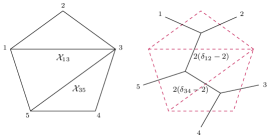
Figure 1: Planar variables and dual skeleton graph for $n=5$.

The planar variables are particularly suited for factorization Goncalves:2014rfa of color-ordered amplitudes. Schematically,

$$\mathcal{M}_{12\cdots n}\sim\frac{\mathcal{M}_{1\cdots(k-1)I}^{(m)}\mathcal{M}_{k\cdots nI}^{(m)}}{\mathcal{X}_{1k}-2m},\quad m=0,1,2,\cdots$$ (13)

where a pole at $\mathcal{X}_{1k}=2m$ corresponds to the exchange of a level-$m$ descendant of $\mathcal{O}$ or $\mathcal{J}$. But we will see in section 5.1, the $m$ can not be the infinity in our story, which indicates a truncation. By induction, all simultaneous poles of $\mathcal{M}_{n}$ consist of compatible planar variables (non-intersecting chords), which gives a partial triangulation of the $n$-gon dual to planar skeleton graphs (Figure 1).

The R-structure decomposition.

Another advantage of working with color-ordered amplitude is a natural basis for the R-charge structures. Let us define a $SU(2)_{R}$ trace as $V_{i_{1}i_{2}\cdots i_{r}}:=\langle i_{1}i_{2}\rangle\langle i_{2}i_{3}\rangle\cdots\langle i_{r}i_{1}\rangle$, where $\langle ij\rangle:=v_{i}^{\alpha}v_{j}^{\beta}\epsilon_{\alpha\beta}\equiv v_{i}\cdot v_{j}$. The Schouten identity $\langle ik\rangle\langle jl\rangle=\langle ij\rangle\langle kl\rangle+\langle il\rangle\langle jk\rangle$ enables us to expand any R-structure to products of non-crossing cycles or $SU(2)_{R}$ traces:

$${\cal M}_{n}^{(s)} =\sum_{\begin{subarray}{c}\text{non-crossing}\\ \text{partition }\pi\\ \text{of }\{1,\cdots,n\}\end{subarray}}\Bigg{(}\prod_{\text{cycle }\tau\,\in\,\pi}V_{\tau}\Bigg{)}M^{(s)}_{n}(\pi),$$ (14)

$${\cal M}_{n}^{(v)\ell} =i\sqrt{2/3}\sum_{\begin{subarray}{c}\text{non-crossing}\\ \text{partition }\pi\\ \text{of }\{1,\cdots,n{-}1\}\end{subarray}}\Bigg{(}\prod_{\text{cycle }\tau\,\in\,\pi}V_{\tau}\Bigg{)}M^{(v)\ell}_{n}(\pi).$$ (15)

For example, (Figure 2)

$$\mathcal{M}_{4}^{(s)} =M_{4}^{(s)}(1234)V_{1234}$$

$$+M_{4}^{(s)}(12;34)V_{12}V_{34}+M_{4}^{(s)}(14;23)V_{14}V_{23},$$

$$\mathcal{M}_{4}^{(v)\ell} =i\sqrt{2/3}M_{4}^{(v)\ell}(123)V_{123},$$

$$\mathcal{M}_{5}^{(s)} =M_{5}^{(s)}(12345)V_{12345}$$

$$+M_{5}^{(s)}(12;345)V_{12}V_{345}+\text{cyclic},$$

$$\mathcal{M}_{5}^{(v)\ell} =i\sqrt{2/3}\left(M_{5}^{(v)\ell}(1234)V_{1234}\right.$$

$$+\left.M_{5}^{(v)\ell}(12;34)V_{12}V_{34}+M_{5}^{(v)\ell}(14;23)V_{14}V_{23}\right).$$

Because a length-$L$ trace picks up $(-)^{L}$ under reflection, for scalar amplitudes this cancels the sign in (4) while for single-gluon amplitudes the net result is a minus sign:

$$M_{4}^{(s)}(12;34) \xlongequal{\text{ref}}M_{4}^{(s)}(21;43)\xlongequal{\text{cyc}}M_{4}^{(s)}(14;23),$$

$$M_{5}^{(v)}(12;34) \xlongequal{\text{ref}}-M_{5}^{(v)}(21;43),$$

$$M_{5}^{(v)}(12;34) \text{ unrelated to }M_{5}^{(v)}(14;23).$$

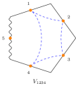
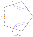
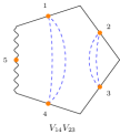
Figure 2: $\mathcal{M}_{5}^{(v)}$ R-structures.

The flat-space limit.

In Alday:2021odx , the authors showed that with $\delta_{ij}=R^{2}s_{ij}$, the leading terms of $\mathcal{M}_{4}^{(s)}$ in the limit $R\to\infty$ is closely related to the color-ordered 4-gluon amplitude. Specifically, setting $\epsilon_{i}\cdot p_{j}=0$ and $\epsilon_{i}\cdot\epsilon_{j}=\langle ij\rangle^{2}=-V_{ij}$,

$$\mathcal{A}_{4}^{\text{flat gluon}}\leadsto V_{12}V_{34}\frac{s_{12}+s_{23}}{s_{12}}+(1\leftrightarrow 3)-V_{13}V_{24}.$$ (16)

Using $V_{13}V_{24}=V_{12}V_{34}+V_{14}V_{23}-2V_{1234}$, this matches the leading terms of $\mathcal{M}_{4}^{(s)}$ (up to overall normalization):

$$\mathcal{M}_{4}^{(s)} =-2\left(\frac{1}{\mathcal{X}_{13}}+\frac{1}{\mathcal{X}_{24}}+1\right)V_{1234}-\frac{\mathcal{X}_{24}-2}{\mathcal{X}_{13}}V_{12}V_{34}-\frac{\mathcal{X}_{13}-2}{\mathcal{X}_{24}}V_{14}V_{23}$$ (17)

$$=-2V_{1234}-\frac{\mathcal{X}_{24}}{\mathcal{X}_{13}}V_{12}V_{34}-\frac{\mathcal{X}_{13}}{\mathcal{X}_{24}}+O(R^{-2}).$$

Here, we argue that this is a general property which holds for any multiplicity, justifying the manipulations in Alday:2023kfm . Recall that, from the bulk perspective, we have a $G_{F}$ gauge theory with adjoint scalars. The scalars are additionally charged under $SU(2)_{R}$, which can be viewed as a flavor symmetry. Importantly, at tree level, the R-symmetry current (which lives in the stress-tensor supermultiplet) decouples, so the flavored scalars must form R-neutral pairs before interacting with the $G_{F}$ gauge field. It is well-known Cachazo:2014xea that, in flat space, flavor-stripped amplitudes of paired scalars in Yang-Mills-flavored-scalar theory can be extracted from pure gluon amplitudes by considering the coefficient of $\epsilon_{i}\cdot\epsilon_{j}$. The flavor-dressed amplitudes are then obtained by dressing each pair with the R-neutral factor $\langle ij\rangle^{2}$. The net result is that we are setting $\epsilon_{i}\cdot p_{j}=0$ and $\epsilon_{i}\cdot\epsilon_{j}=\langle ij\rangle^{2}$ in the pure gluon amplitudes. The result of paired scalar amplitudes have been computed using the CHY formula Cachazo:2013iea explicitly through $n=12$.

The flat-space limit constrains the $R\to\infty$ power-counting of $\mathcal{M}_{n}^{(s)}$. For even $n$, everything is clear, and $\mathcal{M}_{n}^{(s)}\sim\delta^{2-\frac{n}{2}}$. For odd $n$, the flat space amplitude vanishes due to the prescription $\epsilon_{i}\cdot p_{j}=0$. The power counting $s^{2-\frac{n}{2}}$ means that the order $\delta^{2-\lfloor\frac{n}{2}\rfloor}$ vanishes, and $\mathcal{M}_{n}^{(s)}\sim\delta^{2-\lceil\frac{n}{2}\rceil}$.

2.1 Factorization of the Mellin amplitudes

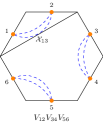
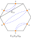
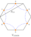
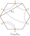
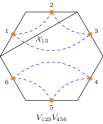
Figure 3: $\mathcal{M}_{6}^{(s)}$ R-structures compatible (above) and incompatible (below) with $\mathcal{X}_{13}$.

Different exchanged fields contribute to different R-structures. For a given channel, say $\mathcal{X}_{1k}$, we distinguish the compatible R-structures (none of the cycles intersect $\mathcal{X}_{1k}$) from the incompatible ones (Figure 3). For scalar exchanges, (13) reads

$$\mathop{\rm Res}_{\mathcal{X}_{1k}=2m}^{(s)}\mathcal{M}_{n}^{(s)}=\mathcal{N}_{s}^{(m)}\texttt{glueR}\left(\mathcal{M}_{1\cdots(k-1)I}^{(s)(m)}\mathcal{M}_{k\cdots nI}^{(s)(m)}\right).$$ (18)

Here, $\mathcal{N}_{s}^{(m)}=-2$, and $\mathcal{M}_{1\cdots(k-1)I}^{(s)(m)}$ is a shifted version of the scalar amplitude $\mathcal{M}_{1\cdots(k-1)I}^{(s)}$:

$$\mathcal{M}_{1\cdots(k-1)I}^{(s)(m)}=\sum_{\begin{subarray}{c}n_{ab}\geq 0\\ \sum n_{ab}=m\end{subarray}}\mathcal{M}_{1\cdots(k-1)I}^{(s)}(\delta_{ab}+n_{ab})\prod_{1\leq a<b<k}\frac{(\delta_{ab})_{n_{ab}}}{n_{ab}!}.$$ (19)

$\mathcal{M}_{k\cdots nI}^{(s)(m)}$ is defined similarly. The operation glueR glues together the traces. Note that there is the 1-1 correspondence of R-structures in amplitudes and OPE:

$$\langle\mathcal{O}(v_{I})\mathcal{O}\cdots\mathcal{O}\rangle\supset\text{something}\times V_{ia\cdots bjI}$$

$$\Updownarrow$$

$$\mathcal{O}\cdots\mathcal{O}\supset\text{something}\times\langle ia\rangle\cdots\langle bj\rangle v_{i}^{(\alpha}v_{j}^{\beta)}\mathcal{O}_{\alpha\beta}$$

Since $\langle\mathcal{O}_{\alpha\beta}\mathcal{O}_{\gamma\delta}\rangle=\frac{1}{2}(\epsilon_{\alpha\gamma}\epsilon_{\beta\delta}+\epsilon_{\alpha\delta}\epsilon_{\beta\gamma})$, we have

$$v_{i}^{(\alpha}v_{j}^{\beta)}v_{k}^{(\gamma}v_{l}^{\delta)}\langle\mathcal{O}_{\alpha\beta}\mathcal{O}_{\gamma\delta}\rangle=\langle il\rangle\langle jk\rangle-\frac{1}{2}\langle ij\rangle\langle lk\rangle.$$ (20)

which implies the following gluing rule:

$$\texttt{glueR}:\ V_{i\cdots jI}\otimes V_{Ik\cdots l}\mapsto V_{i\cdots jk\cdots l}-\frac{1}{2}V_{i\cdots j}V_{k\cdots l}.$$ (21)

We see that scalar exchanges contribute to both compatible and incompatible R-structures. R-structures with more than one cycle intersecting $\mathcal{X}_{1k}$ vanish (Figure 4).

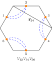
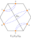
Figure 4: Vanishing R-structures.

For gluon exchanges, (13) reads

$$\mathop{\rm Res}_{\mathcal{X}_{1k}=2m}^{(v)}\mathcal{M}_{n}^{(s)}=\mathcal{N}_{v}^{(m)}\sum_{a=1}^{k-1}\sum_{i=k}^{n}\delta_{ai}\mathcal{M}_{1\cdots(k-1)I}^{(v)(m)a}\mathcal{M}_{k\cdots nI}^{(v)(m)i}.$$ (22)

Here, $\mathcal{N}_{v}^{(m)}=\frac{3}{1+m}$, and $\mathcal{M}_{1\cdots(k-1)I}^{(v)(m)a}$ is $\mathcal{M}_{1\cdots(k-1)I}^{(v)a}$ shifted according to (19). We no longer need glueR because $\mathcal{J}$ is R-neutral; gluon exchanges contribute to compatible R-structures only.

An important consequence of “gauge invariance” (7) is that, at certain no-gluon kinematics, gluon exchanges are forbidden completely. To see this, let us denote $\mathcal{M}_{1\cdots(k-1)I}^{(v)(m)a}\equiv\mathcal{L}^{(m)a}$ and $\mathcal{M}_{k\cdots nI}^{(v)(m)i}\equiv\mathcal{R}^{(m)i}$, and solve $\mathcal{L}^{(m)1},\mathcal{R}^{(m)k}$ using (7). The double sum in (22) becomes

$$\sum_{a=2}^{k-1}\sum_{i=k+1}^{n}\left(\delta_{ai}-\frac{\delta_{aI}}{\delta_{1I}}\delta_{1i}-\frac{\delta_{iI}}{\delta_{kI}}\delta_{ak}+\frac{\delta_{aI}\delta_{iI}}{\delta_{1I}\delta_{kI}}\delta_{1k}\right)\mathcal{L}^{(m)a}\mathcal{R}^{(m)i}.$$

If all $(k-2)(n-k)$ coefficients vanish on the support of $\mathcal{X}_{1k}=2m$, gluon exchanges are forbidden, regardless of the detailed form of $\mathcal{L}^{(m)}$ and $\mathcal{R}^{(m)}$. The number of conditions equals the number of chords $\mathcal{X}_{ai}$ ($2\leq a\leq k-1$ and $k+1\leq i\leq n$) crossing $\mathcal{X}_{1k}$. Hence, the no-gluon conditions translate to $\mathcal{X}_{ai}$ taking special values $\mathcal{X}_{ai}^{*}$:

$$\mathcal{E}_{ai}^{(m)} :=\mathcal{X}_{ai}-\mathcal{X}_{ai}^{*}=0,$$ (23)

$$X_{ai}^{*} =1-m+\frac{\mathcal{X}_{1a}+\mathcal{X}_{1i}+\mathcal{X}_{ak}+\mathcal{X}_{ik}}{2}-\frac{(\mathcal{X}_{1a}-\mathcal{X}_{ak})(\mathcal{X}_{1i}-\mathcal{X}_{ik})}{4(m+1)}.$$ (24)

Since gluon exchanges are forbidden at no-gluon kinematics, scalar exchanges alone fix the residue up to polynomials of $\mathcal{E}$’s:

$$\mathop{\rm Res}_{\mathcal{X}_{1k}=2m}\mathcal{M}_{n}=\left.\mathop{\rm Res}_{\mathcal{X}_{1k}=2m}^{(s)}\mathcal{M}_{n}\right|_{\mathcal{X}_{ai}=\mathcal{X}_{ai}^{*}}+\text{poly}(\mathcal{E}_{ai}^{(m)}).$$ (25)

The special case of (22) where $k=n-1$ is particularly important. From the 3-point single-gluon amplitude :

$$\mathcal{M}_{n-1,n,I}^{(v)(0)n-1}=\frac{i}{\sqrt{6}}V_{n-1,n},\ \mathcal{M}_{n-1,n,I}^{(v)(0)n}=-\frac{i}{\sqrt{6}}V_{n-1,n},$$ (26)

we see that

$$\mathop{\rm Res}_{\mathcal{X}_{1,n-1}=0}^{(v)}\mathcal{M}_{n}^{(s)}=\frac{3i}{\sqrt{6}}V_{n-1,n}\sum_{a=1}^{n-2}(\delta_{a,n-1}-\delta_{a,n})\mathcal{M}_{n-1}^{(v)a}.$$ (27)

This is similar to the scaffolding relation in Arkani-Hamed:2023jry . If we write the $\delta$’s in terms of $\mathcal{X}$’s, one can show that for each $2\leq a\leq n-2$,

$$\mathcal{M}_{n-1}^{(v)a}-\mathcal{M}_{n-1}^{(v)a-1}=\frac{\partial}{\partial\mathcal{X}_{an}}\left(\frac{i\sqrt{2/3}}{V_{n-1,n}}\mathop{\rm Res}_{\mathcal{X}_{1,n-1}=0}^{(v)}\mathcal{M}_{n}^{(s)}\right).$$ (28)

Together with (7), these $(n-3)+1$ equations completely determine $\{\mathcal{M}_{n-1}^{(v)a}\}_{a=1}^{n-2}$. In other words, $(n-1)$-point single-gluon amplitudes can be extracted from the $n$-point scalar amplitude!

3 Constructibility: proof and examples

In Cao:2023cwa , we showed that supergluon amplitudes of any multiplicity can be recursively constructed by alternatingly extracting single-gluon amplitudes and bootstrapping supergluon amplitudes:

(29)

However, we observed in practice that we only need the explicit result of $\mathcal{M}_{5}^{(v)}$ instead of $\mathcal{M}_{6}^{(v)}$ to construct $\mathcal{M}_{8}^{(s)}$. In other words, the above zigzag course can be strengthened:

(30)

In this section, we review and generalize the proof in Cao:2023cwa to explain eq. (30), before demonstrating the algorithm with a $\mathcal{M}_{6}^{(s)}$ example.

3.1 Proof of eq. (29)

The vertical arrows in eq. (29) have already been explained in (28). Here, we need only show the validity of the diagonal arrows.

Suppose we have already obtained the explicit results of $\mathcal{M}_{\leq n-1}^{(s)}$ and $\mathcal{M}_{\leq n-2}^{(v)}$, and we would like to construct $\mathcal{M}_{n}^{(s)}$. We already have enough input to fully constrain the residue of $\mathcal{M}_{n}^{(s)}$ at $\mathcal{X}_{ij}=2m$ where $\|i-j\|\geq 3$ (length$\geq 3$ poles), because both half amplitudes only require $\mathcal{M}_{\leq n-2}$. Note that this determines not just terms with only length$\geq 3$ poles, but all terms with at least one length$\geq 3$ pole. For instance, a term in $\mathcal{M}_{6}^{(s)}$ of the form

$$\frac{\text{something}}{\mathcal{X}_{13}\mathcal{X}_{14}}$$

is visible upon taking the residue at $\mathcal{X}_{14}=0$ and is fixed by factorization.

Terms with only $\mathcal{X}_{i,i+2}=2m$ poles (length-2 poles) are not fixed by factorization, because the gluon-exchange contributions involve $\mathcal{M}_{n-1}^{(v)}$ which is not known by assumption. However, any incompatible R-structure is fixed by scalar factorization, because gluon-exchanges do not contribute (Figure 5). So the remaining problem is to determine terms with only short poles and fully-compatible R-structures (Figure 5(a)). Luckily, no-gluon kinematics enables us to constrain the gluon-exchange contribution without knowing it precisely. It turns out that, together with the flat-space limit, these are sufficient to fully constrain such terms.

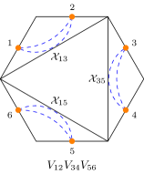
(a)

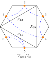
(b)

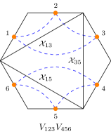
(c)

Figure 5: (a) Not determined by scalar factorization. (b) Determined by scalar factorization at $\mathcal{X}_{13}=0$ or $\mathcal{X}_{35}=0$. (c) Vanish because $\mathcal{X}_{35}$ intersects 2 R-cycles $V_{123}$ and $V_{456}$.

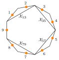
(a)

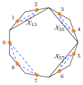
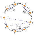
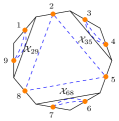
(b)

Figure 6: Odd $n=9$ example. (a) With $n^{\prime}=4$ length-2 poles, any R-cycle involving the 9-th particle necessarily intersect one of the poles. (b) With $n^{\prime}-1=3$ length-2 poles, there is a unique fully compatible R-structure.

Let us try to construct a term (“survivor”) that cannot be fixed by these conditions. We will soon see that this is impossible. As mentioned above, such survivor terms can only have length-2 poles and fully compatible R-structures.

Suppose $n=2n^{\prime}+1$ is odd. The flat-space limit imposes power-counting $\mathcal{X}^{n^{\prime}-1}$, so that each term contains at least $(n^{\prime}-1)$ poles. On the other hand, since each $\mathcal{X}_{ij}$ pole has $\|i-j\|\geq 2$ and incompatible poles are not allowed, there can be at most $n^{\prime}$ poles (all length-2 poles). However, none of the R-structures is simultaneously compatible with $n^{\prime}$ length-2 poles (Figure 6(a)), while a unique R-structure exists for $(n^{\prime}-1)$ length-2 poles (Figure 6(b)). Therefore, a survivor term must have exactly $(n^{\prime}-1)$ length-2 poles, with a constant numerator. But, according to (25), no-gluon kinematics in any one channel (say, $\mathcal{X}_{13}=0$) forces the amplitude to take the form

$$\mathop{\rm Res}_{\mathcal{X}_{13}=0}\mathcal{M}_{n}^{(s)}=\frac{\text{known}+\text{poly}(\mathcal{E}_{2i}^{(0)})}{\text{other denominator factors}},\quad\text{poly}(\mathcal{E}_{2i}^{(0)})\sim\mathcal{X}^{\geq 1}.$$ (31)

In order to survive the no-gluon kinematics constraints, a survivor term must be proportional to $\text{poly}(\mathcal{E})\sim\mathcal{X}^{\geq 1}$, which is impossible with only a constant numerator. As a result, we have just shown that no survivor term exists for odd $n$.

Now, suppose $n=2n^{\prime}$ is even. The flat-space limit imposes power-counting $\mathcal{X}^{n^{\prime}-2}$, so that each term contains at least $(n^{\prime}-2)$ poles. Furthermore, the leading order terms are determined by the flat-space result; in particular, terms with exactly $(n^{\prime}-2)$ poles do not survive the flat-space limit constraint. On the other hand, since each $\mathcal{X}_{ij}$ pole has $\|i-j\|\geq 2$ and incompatible poles are not allowed, there can be at most $n^{\prime}$ poles (all length-2 poles). Hence, multiplying both numerator and denominator by some $\mathcal{X}_{i,i+2}$ and creating spurious poles if necessary, we can put survivor terms into the form

$$\frac{\mathcal{X}^{\leq 1}}{\mathcal{X}^{n^{\prime}}}.$$

For the interesting case of $n^{\prime}\geq 3$, there are at least two (perhaps spurious) poles. It turns out that no such linear numerator can survive no-gluon kinematics constraints in both channels. Let us demonstrate this with an example, and show that no linear numerator $f(\mathcal{X})$ can survive the no-gluon kinematics constraints in both $\mathcal{X}_{13}=0$ and $\mathcal{X}_{35}=0$. To survive the no-gluon kinematics constraint in $\mathcal{X}_{13}=0$,

$$f(\mathcal{X})=\mathcal{X}_{13}\oplus\bigoplus_{i\neq 1,2,3}\mathcal{E}_{2i}^{(0)}=\mathcal{X}_{13}\oplus\bigoplus_{i\neq 1,2,3}\left(\mathcal{X}_{2i}-1-\frac{\mathcal{X}_{1i}+\mathcal{X}_{3i}}{2}\right).$$ (32)

Similarly, to survive the no-gluon kinematics constraint in $\mathcal{X}_{35}=0$,

$$f(\mathcal{X})=\mathcal{X}_{35}\oplus\bigoplus_{i\neq 3,4,5}\mathcal{E}_{4i}^{(0)}=\mathcal{X}_{35}\oplus\bigoplus_{i\neq 3,4,5}\left(\mathcal{X}_{4i}-1-\frac{\mathcal{X}_{3i}+\mathcal{X}_{5i}}{2}\right).$$ (33)

In eq. (32) there are no $\mathcal{X}_{4i}$ except for $i=2$, while in eq. (33) there are no $\mathcal{X}_{2i}$ except for $i=4$. Comparing the terms,

$$f(\mathcal{X})=\mathcal{X}_{13}\oplus\left(\mathcal{X}_{24}-1-\frac{\mathcal{X}_{14}}{2}\right)=\mathcal{X}_{35}\oplus\left(\mathcal{X}_{24}-1-\frac{\mathcal{X}_{25}}{2}\right).$$ (34)

For the interesting case of $n\geq 6$, we have $\mathcal{X}_{1i}\neq\mathcal{X}_{5i}$, so that $f(\mathcal{X})=0$. As a result, we have just shown that no survivor term exists for even $n$.

In summary, we have ruled out the existence of a survivor term not determined by our constraints, and the validity of the diagonal arrows in eq. (29) is established.

3.2 Proof of eq. (30)

The validity of the blue arrows in eq. (30) can be shown in a similar fashion. Since only $\mathcal{M}_{\leq n-3}^{(v)}$ is presumed to be known, survivor terms shoule be constructed with length-2 poles or length-3 poles and fully compatible R-structures.

Suppose $n=2n^{\prime}+1$ is odd. Again, flat-space limit implies that survivor terms have at least $(n^{\prime}-1)$ poles. However, since length-3 poles are allowed, we cannot rule out terms with $n^{\prime}$ poles by compatibility of R-structures (Figure 7). However, to have $n^{\prime}$ poles means to have numerators $\mathcal{X}^{\leq 1}$, and one of the $n^{\prime}$ poles must have length-3. The no-gluon kinematics constraint in the length-3 channel reads

$$\mathop{\rm Res}_{\mathcal{X}_{ii+3}=2m}\mathcal{M}_{n}^{(s)}=\frac{\text{known}+\text{poly}(\mathcal{E})}{\text{other denominator factors}},\quad\text{poly}(\mathcal{E})\sim\mathcal{X}^{\geq 2}.$$ (35)

Importantly, the $\mathcal{E}$ factors are now quadratic, making it impossible to construct a survivor with $\mathcal{X}^{\leq 1}$ numerators. Like before, terms with $(n^{\prime}-1)$ poles and of the form

$$\frac{\text{constant}}{\mathcal{X}^{n^{\prime}-1}}$$

are ruled out by the no-gluon kinematics constraint in any one channel.

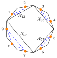
Figure 7: With length-3 poles available, it is possible to have $n^{\prime}$ poles and fully compatible R-structures.

Suppose $n=2n^{\prime}$ is even. Again, flat-space limit implies that survivor terms have at least $(n^{\prime}-1)$ poles. Creating spurious poles as before if necessary, we can put survivor terms into the form

$$\frac{\mathcal{X}^{\leq 1}}{\mathcal{X}^{n^{\prime}}}.$$

Now, if one of the $n^{\prime}$ (perhaps spurious) poles has length 3, the no-gluon kinematics constraint in that channel forces the numerator to be $\text{poly}(\mathcal{E})\sim\mathcal{X}^{\geq 2}$, killing any survivor. On the other hand, if all $n^{\prime}$ (perhaps spurious) poles have length 2, the situation reduces to that discussed in the previous subsection, and we know that no survivors exist.

Therefore, we see that it is not much harder to prove eq.(30) than to prove eq.(29).

3.3 Worked example

Let us illustrate how to use the constructing algorithm in practice with a $\mathcal{M}_{6}^{(s)}$ example. As the arrows in (30) indicates, we will only need the explicit results of $\mathcal{M}_{3}^{(s)},\mathcal{M}_{4}^{(s)},\mathcal{M}_{5}^{(s)}$ and $\mathcal{M}_{3}^{(v)}$.

In the first step, we construct a rational function that has all the correct residues for length$\geq 4$ poles (none for $\mathcal{M}_{6}^{(s)}$) and the correct incompatible-channel contributions for length-2 and length-3 poles, by gluing lower-point amplitudes together using (18). This is achieved by the following observation: suppose we seek a function $F(x,y)$ with only simple poles at $x=0$ and $y=0$ and require

$$\mathop{\rm Res}_{x=0}F(x,y) =F_{x}(y)=\frac{r}{y}+f_{x}(y),$$

$$\mathop{\rm Res}_{y=0}F(x,y) =F_{y}(x)=\frac{r^{\prime}}{x}+f_{y}(x).$$

As long as the input is consistent, i.e., $\mathop{\rm Res}_{x=0}F_{y}(x)=\mathop{\rm Res}_{y=0}F_{x}(y)$ or $r=r^{\prime}$, we can simply take

$$F(x,y)=\frac{F_{x}(y)}{x}+\frac{F_{y}(x)-\frac{\mathop{\rm Res}_{x=0}F_{y}(x)}{x}}{y}\xlongequal{\text{Mathematica}}\frac{F_{x}(y)}{x}+\frac{F_{y}(x)-\left(F_{y}(x)\texttt{/.\{$\frac{1}{x}\to 0$\}}\right)}{y}.$$

Iterating this leads to a simple algorithm that constructs a multi-variate function $\mathcal{S}_{6}^{(s)}$ with correct codim-1 residues. In our particular case, we obtain

$$\frac{S_{6}^{(s)}(123456)}{-8} =\frac{1}{\mathcal{X}_{14}}+\frac{1}{\mathcal{X}_{14}-2}+\frac{1}{\mathcal{X}_{13}\mathcal{X}_{14}}+\frac{1}{\mathcal{X}_{13}\mathcal{X}_{15}}+\frac{1}{\mathcal{X}_{14}\mathcal{X}_{15}}+\frac{1}{\mathcal{X}_{13}\mathcal{X}_{46}}$$

$$+\frac{1}{\mathcal{X}_{13}\mathcal{X}_{14}\mathcal{X}_{15}}+\frac{1}{\mathcal{X}_{13}\mathcal{X}_{35}\mathcal{X}_{15}}+\frac{1}{\mathcal{X}_{14}\mathcal{X}_{15}\mathcal{X}_{24}}+\frac{1}{\mathcal{X}_{15}\mathcal{X}_{24}\mathcal{X}_{25}}$$

$$+\text{their inequivalent cyclic images},$$

$$\frac{S_{6}^{(s)}(123;456)}{4} =\frac{2}{\mathcal{X}_{13}\mathcal{X}_{14}}+\frac{2}{\mathcal{X}_{14}\mathcal{X}_{15}}-\frac{\mathcal{X}_{35}-2}{\mathcal{X}_{13}\mathcal{X}_{14}\mathcal{X}_{15}}-\frac{\mathcal{X}_{25}-2}{\mathcal{X}_{14}\mathcal{X}_{15}\mathcal{X}_{24}}-\frac{\mathcal{X}_{36}-2}{\mathcal{X}_{13}\mathcal{X}_{14}\mathcal{X}_{46}}$$

$$+\text{their inequivalent cyclic-by-3 images},$$

$$\frac{S_{6}^{(s)}(12;34;56)}{-2} =\frac{(\mathcal{X}_{24}-2)(\mathcal{X}_{46}-2)}{\mathcal{X}_{13}\mathcal{X}_{14}\mathcal{X}_{15}}+\frac{(\mathcal{X}_{24}-2)(\mathcal{X}_{46}-2)}{\mathcal{X}_{13}(\mathcal{X}_{14}-2)\mathcal{X}_{15}}$$

$$+\text{their inequivalent cyclic-by-2 images},$$

$$\vdots$$

Notice that $S_{6}^{(s)}(123456)=M_{6}^{(s)}(123456)$ because it does not have compatible channels and gluon-exchange contributions(recall this in Fig. 3).

In the second step, we write down all possible monomials with (a) the correct power-counting, (b) only length-2 and length-3 poles, and (c) fully compatible R-structures. In our case, we have the following list of possible monomials:

$$V_{123456}: \quad\text{none},$$

$$V_{12}V_{3456}: \quad\frac{1}{\mathcal{X}_{13}},$$

$$V_{123}V_{456}: \quad\frac{1}{\mathcal{X}_{14}},\ \frac{1}{\mathcal{X}_{14}-2},$$

$$V_{14}V_{23}V_{56}: \quad\frac{1}{\mathcal{X}_{15}},\ \frac{1}{\mathcal{X}_{24}},\ \frac{1}{\mathcal{X}_{15}\mathcal{X}_{24}},\ \frac{\mathcal{X}_{13}}{\mathcal{X}_{15}\mathcal{X}_{24}},\ \frac{\mathcal{X}_{14}}{\mathcal{X}_{15}\mathcal{X}_{24}},\ \frac{\mathcal{X}_{25}}{\mathcal{X}_{15}\mathcal{X}_{24}},\ \frac{\mathcal{X}_{26}}{\mathcal{X}_{15}\mathcal{X}_{24}},$$

$$\quad\frac{\mathcal{X}_{35}}{\mathcal{X}_{15}\mathcal{X}_{24}},\ \frac{\mathcal{X}_{36}}{\mathcal{X}_{15}\mathcal{X}_{24}},\ \frac{\mathcal{X}_{46}}{\mathcal{X}_{15}\mathcal{X}_{24}},$$

$$V_{12}V_{34}V_{56}: \quad\frac{1}{\mathcal{X}_{13}},\ \frac{1}{\mathcal{X}_{13}\mathcal{X}_{35}},\ \frac{\mathcal{X}_{14}}{\mathcal{X}_{13}\mathcal{X}_{35}},\ \frac{\mathcal{X}_{15}}{\mathcal{X}_{13}\mathcal{X}_{35}},\ \frac{\mathcal{X}_{24}}{\mathcal{X}_{13}\mathcal{X}_{35}},\ \frac{\mathcal{X}_{25}}{\mathcal{X}_{13}\mathcal{X}_{35}},\ \frac{\mathcal{X}_{26}}{\mathcal{X}_{13}\mathcal{X}_{35}},$$

$$\quad\frac{\mathcal{X}_{36}}{\mathcal{X}_{13}\mathcal{X}_{35}},\ \frac{\mathcal{X}_{46}}{\mathcal{X}_{13}\mathcal{X}_{35}},\ \frac{1}{\mathcal{X}_{13}\mathcal{X}_{35}\mathcal{X}_{15}},\ \frac{\mathcal{X}_{14}}{\mathcal{X}_{13}\mathcal{X}_{35}\mathcal{X}_{15}},\ \frac{\mathcal{X}_{24}}{\mathcal{X}_{13}\mathcal{X}_{35}\mathcal{X}_{15}},\ \frac{\mathcal{X}_{14}\mathcal{X}_{24}}{\mathcal{X}_{13}\mathcal{X}_{35}\mathcal{X}_{15}},$$

$$\quad\frac{\mathcal{X}_{14}\mathcal{X}_{25}}{\mathcal{X}_{13}\mathcal{X}_{35}\mathcal{X}_{15}},\ \frac{\mathcal{X}_{14}\mathcal{X}_{26}}{\mathcal{X}_{13}\mathcal{X}_{35}\mathcal{X}_{15}},\ \frac{\mathcal{X}_{24}\mathcal{X}_{25}}{\mathcal{X}_{13}\mathcal{X}_{35}\mathcal{X}_{15}},\ \frac{\mathcal{X}_{24}\mathcal{X}_{26}}{\mathcal{X}_{13}\mathcal{X}_{35}\mathcal{X}_{15}},$$

$$\quad\text{and their inequivalent cyclic-by-2 images}.$$

In the third step, we write down the most general linear combination $\sum\text{coef}(\text{term})\times\text{term}$ of the above monomials, and add it to $\mathcal{S}_{6}^{(s)}$. Demanding the result has the correct flat-space limit fixes a bunch of terms. In our particular case, flat-space limit fixes

$$\text{coef}\left(V_{12}V_{34}V_{56}\frac{\mathcal{X}_{14}}{\mathcal{X}_{13}\mathcal{X}_{35}}\right)=0,\quad\text{coef}\left(V_{12}V_{34}V_{56}\frac{\mathcal{X}_{24}}{\mathcal{X}_{13}\mathcal{X}_{35}}\right)=-4,$$

$$\text{coef}\left(V_{123}V_{456}\frac{1}{\mathcal{X}_{14}}\right)+\text{coef}\left(V_{123}V_{456}\frac{1}{\mathcal{X}_{14}-2}\right)=8,\quad\text{etc.}$$

In other words, the unfixed terms are those subleading in the large-$\mathcal{X}$ limit:

$$V_{123456}: \quad\text{none},$$

$$V_{12}V_{3456}: \quad\text{none},$$

$$V_{123}V_{456}: \quad\frac{1}{\mathcal{X}_{14}}-\frac{1}{\mathcal{X}_{14}-2},$$

$$V_{14}V_{23}V_{56}: \quad\frac{1}{\mathcal{X}_{15}\mathcal{X}_{24}},$$

$$V_{12}V_{34}V_{56}: \quad\frac{1}{\mathcal{X}_{13}\mathcal{X}_{35}},\ \frac{1}{\mathcal{X}_{13}\mathcal{X}_{35}\mathcal{X}_{15}},\ \frac{\mathcal{X}_{14}}{\mathcal{X}_{13}\mathcal{X}_{35}\mathcal{X}_{15}},\ \frac{\mathcal{X}_{24}}{\mathcal{X}_{13}\mathcal{X}_{35}\mathcal{X}_{15}},$$

$$\quad\text{and their inequivalent cyclic-by-2 images}.$$

In the fourth and final step, we consider the no-gluon kinematics in each factorization channel. For instance, consider the ansatz for $M_{6}^{(s)}(12;34;56)$ which now reads:

$$M_{6}^{(s)}(12;34;56) =\frac{-2(\mathcal{X}_{24}-2)(\mathcal{X}_{46}-2)}{\mathcal{X}_{13}\mathcal{X}_{14}\mathcal{X}_{15}}+\frac{-2(\mathcal{X}_{24}-2)(\mathcal{X}_{46}-2)}{\mathcal{X}_{13}(\mathcal{X}_{14}-2)\mathcal{X}_{15}}$$

$$+\frac{c_{1}-4\mathcal{X}_{14}+4\mathcal{X}_{24}-4\mathcal{X}_{26}+4\mathcal{X}_{46}}{\mathcal{X}_{13}\mathcal{X}_{15}}+\frac{c_{2}}{\mathcal{X}_{13}\mathcal{X}_{35}\mathcal{X}_{15}}$$

$$+\frac{c_{3}\mathcal{X}_{14}+c_{4}\mathcal{X}_{24}+4\mathcal{X}_{14}\mathcal{X}_{25}-4\mathcal{X}_{14}\mathcal{X}_{26}}{\mathcal{X}_{13}\mathcal{X}_{35}\mathcal{X}_{15}}$$

$$+\text{their inequivalent cyclic-by-2 images}.$$

The no-gluon kinematics for the compatible channel $\mathcal{X}_{13}=0$ reads (23),

$$\mathcal{X}_{24} =1+\frac{\mathcal{X}_{14}}{2},$$

$$\mathcal{X}_{25} =1+\frac{\mathcal{X}_{15}+\mathcal{X}_{35}}{2},$$

$$\mathcal{X}_{26} =1+\frac{\mathcal{X}_{36}}{2}.$$

Taking the residue and evaluating at the no-gluon kinematics,

$$\mathop{\rm Res}_{\mathcal{X}_{13}=0}M_{6}^{(s)}(12;34;56)\Big{|}_{\text{no-gluon}} =\frac{4+c_{1}+\frac{1}{2}c_{3}}{\mathcal{X}_{15}}+\frac{4+c_{1}+\frac{1}{2}c_{3}}{\mathcal{X}_{35}}+\frac{2(\mathcal{X}_{46}-2)}{\mathcal{X}_{14}\mathcal{X}_{15}}+\frac{2(\mathcal{X}_{46}-2)}{\mathcal{X}_{35}\mathcal{X}_{36}}$$

$$+\frac{c_{2}+c_{3}+2c_{4}+(c_{3}+\frac{1}{2}c_{4})\mathcal{X}_{14}+(c_{3}+\frac{1}{2}c_{4})\mathcal{X}_{36}+(c_{4}-4)\mathcal{X}_{46}}{\mathcal{X}_{15}\mathcal{X}_{35}}.$$

On the other hand, we know that the correct result should match the scalar-exchange contribution obtained through gluing $\mathcal{M}_{3}^{(s)}\otimes\mathcal{M}_{5}^{(s)}$:

$$\mathop{\rm Res}_{\mathcal{X}_{13}=0}\mathcal{M}_{6}^{(s)}\Big{|}_{\text{no-gluon}} =-2\texttt{glueR}\left(\mathcal{M}_{12I}^{(s)(0)}\mathcal{M}_{3456I}^{(s)(0)}\right)\Big{|}_{\text{no-gluon}}$$

$$=V_{12}V_{34}V_{56}\left(\frac{-4}{\mathcal{X}_{15}}+\frac{-4}{\mathcal{X}_{35}}+\frac{2(\mathcal{X}_{46}-2)}{\mathcal{X}_{14}\mathcal{X}_{15}}+\frac{2(\mathcal{X}_{46}-2)}{\mathcal{X}_{35}\mathcal{X}_{36}}-\frac{2(4-\mathcal{X}_{14}-\mathcal{X}_{36})}{\mathcal{X}_{15}\mathcal{X}_{35}}\right)$$

$$+\text{other R-structures}.$$

Comparing the coefficients, we see that

$$c_{1}=-8,\quad c_{2}=-16,\quad c_{3}=0,\quad c_{4}=4.$$

For this particular example, one channel suffices. In general, we need to consider every factorization channel to completely fix the answer. In the end, we arrive at

$$M_{6}^{(s)}(12;34;56) =\frac{-2(\mathcal{X}_{24}-2)(\mathcal{X}_{46}-2)}{\mathcal{X}_{13}\mathcal{X}_{14}\mathcal{X}_{15}}+\frac{-2(\mathcal{X}_{24}-2)(\mathcal{X}_{46}-2)}{\mathcal{X}_{13}(\mathcal{X}_{14}-2)\mathcal{X}_{15}}$$

$$+\frac{-8-4\mathcal{X}_{14}+4\mathcal{X}_{24}-4\mathcal{X}_{26}+4\mathcal{X}_{46}}{\mathcal{X}_{13}\mathcal{X}_{15}}+\frac{-16}{\mathcal{X}_{13}\mathcal{X}_{35}\mathcal{X}_{15}}$$

$$+\frac{4\mathcal{X}_{24}+4\mathcal{X}_{14}\mathcal{X}_{25}-4\mathcal{X}_{14}\mathcal{X}_{26}}{\mathcal{X}_{13}\mathcal{X}_{35}\mathcal{X}_{15}}$$

$$+\text{their inequivalent cyclic-by-2 images}.$$

4 Explicit results for supergluon and spinning amplitudes

For convenience, we record explicit, human-readable results for supergluon amplitudes up to $n=7$ and spinning amplitudes up to $n=6$. All these and some higher-point results can be found in the ancillary file of Cao:2023cwa , but we present these compact formula mainly to show how simple these amplitudes actually are and to make their interesting mathematical structures more visible. The $n=4,5$ supergluon amplitudes can be found in Alday:2021odx ; Alday:2022lkk , so we start with $n=6$ supergluon amplitudes:

$$\frac{M_{6}(123456)}{-8} =\left[\left(\frac{1}{{\cal X}_{14}}+\frac{1}{{\cal X}_{14}-2}\right)+2\leavevmode\nobreak\ {\rm cyclic}\right]$$

$$+\left[\left(\frac{1}{{\cal X}_{13}{\cal X}_{14}}+\frac{1}{{\cal X}_{13}{\cal X}_{15}}+\frac{1}{{\cal X}_{14}{\cal X}_{15}}\right)+5\leavevmode\nobreak\ {\rm cyclic}+\frac{1}{{\cal X}_{13}{\cal X}_{46}}+2\leavevmode\nobreak\ {\rm cyclic}\right]$$

$$+\left[\left(\frac{1}{{\cal X}_{13}{\cal X}_{14}{\cal X}_{15}}+\frac{1}{{\cal X}_{13}{\cal X}_{14}{\cal X}_{46}}\right)+5\leavevmode\nobreak\ {\rm cyclic}+\frac{1}{{\cal X}_{13}{\cal X}_{15}{\cal X}_{35}}+1\leavevmode\nobreak\ {\rm cyclic}\right]\!,\!$$ (36)

$$\frac{M_{6}(12;3456)}{4} =\frac{1}{{\cal X}_{13}}\left[\,2+\frac{2}{{\cal X}_{15}}+\frac{2}{{\cal X}_{35}}+\frac{2}{{\cal X}_{46}}-\frac{{\cal X}_{25}-2}{{\cal X}_{15}{\cal X}_{35}}\right.$$

$$\hskip 37.00002pt\left.-\,({\cal X}_{24}-2)\left(\frac{1}{{\cal X}_{14}}+\frac{1}{{\cal X}_{14}-2}+\frac{1}{{\cal X}_{14}{\cal X}_{15}}+\frac{1}{{\cal X}_{14}{\cal X}_{46}}\right)\right.$$

$$\hskip 37.00002pt\left.-\,({\cal X}_{26}-2)\left(\frac{1}{{\cal X}_{36}}+\frac{1}{{\cal X}_{36}-2}+\frac{1}{{\cal X}_{36}{\cal X}_{46}}+\frac{1}{{\cal X}_{35}{\cal X}_{36}}\right)\right],$$ (37)

$$\frac{M_{6}(123;456)}{4} =\frac{1}{{\cal X}_{14}-2}+\frac{1}{{\cal X}_{14}}\left(1+\frac{2}{{\cal X}_{13}}+\frac{2}{{\cal X}_{15}}+\frac{2}{{\cal X}_{24}}+\frac{2}{{\cal X}_{46}}\right.$$

$$\hskip 85.00012pt-\left.\frac{{\cal X}_{25}-2}{{\cal X}_{15}{\cal X}_{24}}-\frac{{\cal X}_{35}-2}{{\cal X}_{13}{\cal X}_{15}}-\frac{{\cal X}_{26}-2}{{\cal X}_{24}{\cal X}_{46}}-\frac{{\cal X}_{36}-2}{{\cal X}_{13}{\cal X}_{46}}\right),$$ (38)

$$\frac{M_{6}(12;36;45)}{-2} =\frac{1}{{\cal X}_{13}{\cal X}_{46}}\left(8-2{\cal X}_{25}+\frac{\left({\cal X}_{15}-2\right)\left({\cal X}_{24}-2\right)}{{\cal X}_{14}}+\frac{\left({\cal X}_{15}-2\right)\left({\cal X}_{24}-2\right)}{{\cal X}_{14}-2}\right.$$

$$\hskip 55.00008pt\left.+\,\frac{\left({\cal X}_{26}-2\right)\left({\cal X}_{35}-2\right)}{{\cal X}_{36}}+\frac{\left({\cal X}_{26}-2\right)\left({\cal X}_{35}-2\right)}{{\cal X}_{36}-2}\right),$$ (39)

$$\frac{M_{6}(12;34;56)}{-2} =\left[\frac{1}{{\cal X}_{13}{\cal X}_{15}}\left(2\left({\cal X}_{14}-{\cal X}_{24}+{\cal X}_{26}-{\cal X}_{46}+2\right)\phantom{\frac{\left({\cal X}_{24}-2\right)\left({\cal X}_{46}-2\right)}{{\cal X}_{14}}}\right.\right.$$

$$\hskip 60.00009pt\left.\left.+\,\frac{\left({\cal X}_{24}-2\right)\left({\cal X}_{46}-2\right)}{{\cal X}_{14}}+\frac{\left({\cal X}_{24}-2\right)\left({\cal X}_{46}-2\right)}{{\cal X}_{14}-2}\right)+2\text{ cyclic}\right]$$

$$+\frac{2}{{\cal X}_{13}{\cal X}_{15}{\cal X}_{35}}\left(\begin{aligned} &4-{\cal X}_{46}-{\cal X}_{24}-{\cal X}_{26}+{\cal X}_{36}{\cal X}_{24}-{\cal X}_{14}{\cal X}_{25}\\ &+{\cal X}_{14}{\cal X}_{26}-{\cal X}_{14}{\cal X}_{36}-{\cal X}_{25}{\cal X}_{36}+{\cal X}_{25}{\cal X}_{46}\end{aligned}\right).$$ (40)

Next we give $n=7$ supergluon amplitudes:

$$\frac{M_{7}(1234567)}{16} =\left[\left(\frac{1}{\mathcal{X}_{13}\mathcal{X}_{15}}+\frac{1}{\mathcal{X}_{13}\left(\mathcal{X}_{15}-2\right)}+\frac{1}{\mathcal{X}_{13}\mathcal{X}_{14}\mathcal{X}_{15}}+\frac{1}{\mathcal{X}_{13}\mathcal{X}_{14}\mathcal{X}_{16}}\right.\right.$$

$$\hskip 20.00003pt\left.\left.+\frac{1}{\mathcal{X}_{14}\mathcal{X}_{15}\mathcal{X}_{24}}+\frac{1}{\mathcal{X}_{14}\mathcal{X}_{16}\mathcal{X}_{24}}+\frac{1}{\mathcal{X}_{15}\mathcal{X}_{16}\mathcal{X}_{24}}\right.\right.$$

$$\hskip 20.00003pt\left.\left.+\frac{1}{\mathcal{X}_{14}\mathcal{X}_{15}\mathcal{X}_{16}\mathcal{X}_{24}}+\frac{1}{\mathcal{X}_{13}\mathcal{X}_{15}\mathcal{X}_{16}\mathcal{X}_{35}}\right)+14\leavevmode\nobreak\ \text{dihedral}\right],$$ (41)

$$\frac{M_{7}(123;4567)}{-8} =\left\{\frac{1}{\mathcal{X}_{14}}\left[\frac{2}{\mathcal{X}_{15}}+\frac{1}{\mathcal{X}_{15}-2}+\frac{1}{\mathcal{X}_{16}}+\frac{1/2}{\mathcal{X}_{57}}+\frac{2}{\mathcal{X}_{13}}-\frac{\mathcal{X}_{26}-2}{\mathcal{X}_{16}\mathcal{X}_{24}\mathcal{X}_{46}}\right.\right.$$

$$\hskip 33.00008pt-\left(\frac{\mathcal{X}_{25}-2}{\mathcal{X}_{24}}+\frac{\mathcal{X}_{35}-2}{\mathcal{X}_{13}}\right)\left(\frac{1}{\mathcal{X}_{15}}+\frac{1}{\mathcal{X}_{15}-2}+\frac{1}{\mathcal{X}_{15}\mathcal{X}_{16}}+\frac{1}{\mathcal{X}_{15}\mathcal{X}_{57}}\right)$$

$$\hskip 36.0001pt+\left.\frac{2}{\mathcal{X}_{15}\mathcal{X}_{16}}+\frac{2}{\mathcal{X}_{16}\mathcal{X}_{24}}+\frac{2}{\mathcal{X}_{13}\mathcal{X}_{57}}+\frac{2}{\mathcal{X}_{15}\mathcal{X}_{57}}+\frac{2}{\mathcal{X}_{13}\mathcal{X}_{16}}+\frac{1}{\mathcal{X}_{16}\mathcal{X}_{46}}\right]$$

$$\hskip 15.00002pt+\left.\frac{1}{\mathcal{X}_{14}-2}\left(\frac{1}{\mathcal{X}_{16}}+\frac{1}{\mathcal{X}_{15}-2}+\frac{1/2}{\mathcal{X}_{57}}\right)\right\}+(1\leftrightarrow 4,2\leftrightarrow 3,5\leftrightarrow 7),$$ (42)

$$\frac{M_{7}(14;23;567)}{4} =\frac{1}{\mathcal{X}_{24}}\left[\frac{4}{\mathcal{X}_{15}}+\frac{2}{\mathcal{X}_{15}-2}+\frac{\mathcal{X}_{13}-2}{\mathcal{X}_{14}\mathcal{X}_{15}}\left(\frac{\mathcal{X}_{46}-2}{\mathcal{X}_{16}}+\frac{\mathcal{X}_{47}-2}{\mathcal{X}_{57}}-2\right)\right.$$

$$\hskip 33.00008pt-\frac{\mathcal{X}_{13}-2}{\mathcal{X}_{14}-2}\left(\frac{1}{\mathcal{X}_{15}}+\frac{1}{\mathcal{X}_{15}-2}-\frac{\mathcal{X}_{46}-2}{\mathcal{X}_{15}\mathcal{X}_{16}}-\frac{\mathcal{X}_{47}-2}{\mathcal{X}_{15}\mathcal{X}_{57}}\right)$$

$$\hskip 33.00008pt-\frac{2\mathcal{X}_{37}-8}{\mathcal{X}_{15}\mathcal{X}_{57}}-\frac{2\mathcal{X}_{36}-8}{\mathcal{X}_{15}\mathcal{X}_{16}}+\frac{\mathcal{X}_{35}-2}{\mathcal{X}_{15}\mathcal{X}_{25}}\left(\frac{\mathcal{X}_{26}-2}{\mathcal{X}_{16}}+\frac{\mathcal{X}_{27}-2}{\mathcal{X}_{57}}-2\right)$$

$$\hskip 33.00008pt\left.-\frac{\mathcal{X}_{35}-2}{\mathcal{X}_{25}-2}\left(\frac{1}{\mathcal{X}_{15}}+\frac{1}{\mathcal{X}_{15}-2}+\frac{\mathcal{X}_{26}-2}{\mathcal{X}_{15}\mathcal{X}_{16}}+\frac{\mathcal{X}_{27}-2}{\mathcal{X}_{15}\mathcal{X}_{57}}\right)\right].$$ (43)

$$\frac{M_{7}(12;34567)}{-8} =\frac{1}{\mathcal{X}_{13}}\left[\frac{2}{\mathcal{X}_{15}}+\frac{2}{\mathcal{X}_{15}-2}+\frac{2}{\mathcal{X}_{16}}+\frac{2}{\mathcal{X}_{46}}+\frac{1}{\mathcal{X}_{47}}+\frac{1}{\mathcal{X}_{47}-2}-\frac{\mathcal{X}_{25}-2}{\left(\mathcal{X}_{15}-2\right)\mathcal{X}_{35}}\right.$$

$$\hskip 37.00002pt+\frac{1}{\mathcal{X}_{16}\mathcal{X}_{35}}+\frac{2}{\mathcal{X}_{15}\mathcal{X}_{16}}+\frac{2}{\mathcal{X}_{16}\mathcal{X}_{46}}+\frac{2}{\mathcal{X}_{36}\mathcal{X}_{46}}+\frac{2}{\mathcal{X}_{47}\mathcal{X}_{57}}$$

$$\hskip 37.00002pt-\frac{\mathcal{X}_{24}-2}{\mathcal{X}_{14}}\left(\frac{1}{\mathcal{X}_{15}}+\frac{1}{\mathcal{X}_{16}}+\frac{1}{\mathcal{X}_{46}}+\frac{1}{\mathcal{X}_{47}}+\frac{1}{\mathcal{X}_{57}}\right.$$

$$\hskip 75.0001pt\left.+\frac{1}{\mathcal{X}_{15}\mathcal{X}_{16}}+\frac{1}{\mathcal{X}_{16}\mathcal{X}_{46}}+\frac{1}{\mathcal{X}_{46}\mathcal{X}_{47}}+\frac{1}{\mathcal{X}_{47}\mathcal{X}_{57}}+\frac{1}{\mathcal{X}_{57}\mathcal{X}_{15}}\right)$$

$$\hskip 37.00002pt-\frac{\mathcal{X}_{24}-2}{\mathcal{X}_{14}-2}\left(\frac{1}{\mathcal{X}_{15}-2}+\frac{1}{\mathcal{X}_{16}}+\frac{1}{\mathcal{X}_{46}}+\frac{1}{\mathcal{X}_{47}-2}+\frac{1}{\mathcal{X}_{57}}\right)$$

$$\hskip 37.00002pt\left.-\frac{\mathcal{X}_{25}-2}{\mathcal{X}_{15}\mathcal{X}_{35}}\left(\frac{1}{\mathcal{X}_{57}}+\frac{1}{\mathcal{X}_{16}}+1\right)\right]+(1\leftrightarrow 3,4\leftrightarrow 7,5\leftrightarrow 6),$$ (44)

$$\frac{M_{7}(12;34;567)}{4} =\left\{\frac{1}{\mathcal{X}_{13}}\left[\frac{2}{\mathcal{X}_{15}}+\frac{2}{\mathcal{X}_{15}-2}-\frac{\mathcal{X}_{24}-2}{\mathcal{X}_{14}-2}\left(\frac{1}{\mathcal{X}_{15}}+\frac{1}{\mathcal{X}_{15}-2}\right)-\frac{2\left(\mathcal{X}_{24}-2\right)}{\mathcal{X}_{14}\mathcal{X}_{15}}\right.\right.$$

$$\hskip 33.00008pt-\frac{\mathcal{X}_{27}-2}{\mathcal{X}_{35}}\left(\frac{2}{\mathcal{X}_{37}}+\frac{2}{\mathcal{X}_{37}-2}-\frac{\mathcal{X}_{46}-2}{2\mathcal{X}_{36}\mathcal{X}_{37}}-\frac{\mathcal{X}_{46}-2}{2\left(\mathcal{X}_{36}-2\right)\left(\mathcal{X}_{37}-2\right)}\right)$$

$$\hskip 33.00008pt+\frac{3}{\mathcal{X}_{35}}-\frac{\mathcal{X}_{14}-\mathcal{X}_{24}+\mathcal{X}_{26}-\mathcal{X}_{46}+2}{\mathcal{X}_{15}\mathcal{X}_{16}}-\frac{\mathcal{X}_{14}+\mathcal{X}_{25}-4}{2\left(\mathcal{X}_{15}-2\right)\mathcal{X}_{35}}$$

$$\hskip 33.00008pt\left.+\frac{\mathcal{X}_{14}-\mathcal{X}_{24}+\mathcal{X}_{27}-\mathcal{X}_{47}+2}{\mathcal{X}_{15}\mathcal{X}_{57}}-\frac{\mathcal{X}_{14}+2\mathcal{X}_{24}+\mathcal{X}_{25}-8}{2\mathcal{X}_{15}\mathcal{X}_{35}}\right]$$

$$\hskip 15.00002pt+\frac{\mathcal{X}_{24}-\mathcal{X}_{25}+\mathcal{X}_{26}-\mathcal{X}_{46}-2}{\mathcal{X}_{15}\mathcal{X}_{16}\mathcal{X}_{35}}-\frac{\mathcal{X}_{24}-\mathcal{X}_{25}+\mathcal{X}_{27}-\mathcal{X}_{47}-2}{\mathcal{X}_{15}\mathcal{X}_{35}\mathcal{X}_{57}}$$

$$\hskip 15.00002pt\left.-\frac{M_{6}(12;34;56)}{2\mathcal{X}_{16}}\right\}+(1\leftrightarrow 5,2\leftrightarrow 4,6\leftrightarrow 7).$$ (45)

$$\frac{M_{7}(12;56;347)}{4} =\frac{1}{\mathcal{X}_{13}\mathcal{X}_{57}}\left[6+\frac{\mathcal{X}_{16}-2}{\mathcal{X}_{15}}\left(\frac{\mathcal{X}_{24}-2}{\mathcal{X}_{14}}+\frac{\mathcal{X}_{25}-2}{\mathcal{X}_{35}}-2\right)-\frac{2(\mathcal{X}_{46}-2)}{\mathcal{X}_{47}}\right.$$

$$\hskip 50.00008pt+\frac{\mathcal{X}_{16}-2}{\mathcal{X}_{15}-2}\left(\frac{\mathcal{X}_{24}-2}{\mathcal{X}_{14}-2}+\frac{\mathcal{X}_{25}-2}{\mathcal{X}_{35}}-2\right)+\frac{\mathcal{X}_{24}-2}{\mathcal{X}_{14}}\left(\frac{\mathcal{X}_{46}-2}{\mathcal{X}_{47}}-2\right)$$

$$\hskip 50.00008pt+\frac{\mathcal{X}_{46}-2}{\mathcal{X}_{47}-2}\left(\frac{\mathcal{X}_{24}-2}{\mathcal{X}_{14}-2}+\frac{\mathcal{X}_{27}-2}{\mathcal{X}_{37}-2}-2\right)+\frac{\mathcal{X}_{27}-2}{\mathcal{X}_{37}-2}\left(\frac{\mathcal{X}_{36}-2}{\mathcal{X}_{35}}-2\right)$$

$$\hskip 50.00008pt\left.+\frac{\mathcal{X}_{27}-2}{\mathcal{X}_{37}}\left(\frac{\mathcal{X}_{36}-2}{\mathcal{X}_{35}}+\frac{\mathcal{X}_{46}-2}{\mathcal{X}_{47}}-2\right)-\frac{2\mathcal{X}_{26}-8}{\mathcal{X}_{35}}\right].$$ (46)

We also present all spinning amplitudes for $n=3,4,5,6$.

$$2M^{(v)}_{3}(12) =\texttt{zp[$1$]}-\texttt{zp[$2$]},$$ (47)

$$M^{(v)}_{4}(123) =-\frac{\texttt{zp[$1$]}-\texttt{zp[$23$]}}{\mathcal{X}_{24}}-\frac{\texttt{zp[$12$]}-\texttt{zp[$3$]}}{\mathcal{X}_{13}},$$ (48)

$$\frac{M^{(v)}_{5}(1234)}{2} =\,\frac{2\texttt{zp[$1$]}}{\mathcal{X}_{25}-2}+\frac{\texttt{zp[$1$]}-\texttt{zp[$234$]}}{\mathcal{X}_{25}}\left(\frac{1}{\mathcal{X}_{35}}+\frac{1}{\mathcal{X}_{24}}+1\right)+\frac{\texttt{zp[$12$]}-\texttt{zp[$34$]}}{\mathcal{X}_{13}\mathcal{X}_{35}}$$

$$\hskip 10.00002pt-\frac{2\texttt{zp[$4$]}}{\mathcal{X}_{14}-2}+\frac{\texttt{zp[$123$]}-\texttt{zp[$4$]}}{\mathcal{X}_{14}}\left(\frac{1}{\mathcal{X}_{24}}+\frac{1}{\mathcal{X}_{13}}+1\right),$$ (49)

$$M^{(v)}_{5}(12;34) =\,\frac{2\texttt{zp[$1$]}\left(\mathcal{X}_{24}-2\right)}{\left(\mathcal{X}_{25}-2\right)\mathcal{X}_{35}}-\frac{(\texttt{zp[$1$]}-\texttt{zp[$234$]})\left(\mathcal{X}_{24}-2\right)}{\mathcal{X}_{25}\mathcal{X}_{35}}$$

$$\hskip 10.00002pt-\frac{2\texttt{zp[$4$]}\left(\mathcal{X}_{24}-2\right)}{\mathcal{X}_{13}\left(\mathcal{X}_{14}-2\right)}+\frac{(\texttt{zp[$123$]}-\texttt{zp[$4$]})\left(\mathcal{X}_{24}-2\right)}{\mathcal{X}_{13}\mathcal{X}_{14}}$$

$$\hskip 10.00002pt+\frac{1}{\mathcal{X}_{13}\mathcal{X}_{35}}\left(\begin{gathered}-4(\texttt{zp[$1$]}-\texttt{zp[$4$]})+2\mathcal{X}_{24}(\texttt{zp[$12$]}-\texttt{zp[$34$]})\\ +\mathcal{X}_{25}(3\texttt{zp[$3$]}-\texttt{zp[$124$]})+\mathcal{X}_{14}(\texttt{zp[$134$]}-3\texttt{zp[$2$]})\end{gathered}\right)$$ (52)

$$\hskip 10.00002pt+2(\texttt{zp[$14$]}-\texttt{zp[$23$]})\left(\frac{1}{\mathcal{X}_{13}}-\frac{1}{\mathcal{X}_{35}}\right),$$ (53)

$$M_{5}^{(v)}(14;23) =\frac{2\texttt{zp[$1$]}(\mathcal{X}_{35}-2)}{\mathcal{X}_{24}(\mathcal{X}_{25}-2)}+\frac{(\mathcal{X}_{35}-2)(\texttt{zp[$1$]}-\texttt{zp[$234$]})}{\mathcal{X}_{24}\mathcal{X}_{25}}-\frac{2(\texttt{zp[$12$]}-\texttt{zp[$34$]})}{\mathcal{X}_{24}}$$

$$-\frac{2\texttt{zp[$4$]}(\mathcal{X}_{13}-2)}{(\mathcal{X}_{14}-2)\mathcal{X}_{24}}-\frac{(\mathcal{X}_{13}-2)(\texttt{zp[$4$]}-\texttt{zp[$123$]})}{\mathcal{X}_{14}\mathcal{X}_{24}}.$$ (54)

$$\frac{M^{(v)}_{6}(12345)}{4} =-\,\frac{2\texttt{zp[$1$]}}{\mathcal{X}_{26}-2}\left(\frac{1}{\mathcal{X}_{25}-2}+\frac{1}{\mathcal{X}_{35}}+\frac{1}{\mathcal{X}_{36}-2}+\frac{1}{\mathcal{X}_{46}}+\frac{1}{\mathcal{X}_{24}}\right)-\frac{2\texttt{zp[$12$]}}{\mathcal{X}_{13}\left(\mathcal{X}_{36}-2\right)}$$

$$\hskip 10.00002pt+\frac{2\texttt{zp[$5$]}}{\mathcal{X}_{15}-2}\left(\frac{1}{\mathcal{X}_{14}-2}+\frac{1}{\mathcal{X}_{24}}+\frac{1}{\mathcal{X}_{25}-2}+\frac{1}{\mathcal{X}_{35}}+\frac{1}{\mathcal{X}_{13}}\right)+\frac{2\texttt{zp[$45$]}}{\left(\mathcal{X}_{14}-2\right)\mathcal{X}_{46}}$$

$$\hskip 10.00002pt-\frac{\texttt{zp[$1234$]}-\texttt{zp[$5$]}}{\mathcal{X}_{15}}\frac{M_{5}^{(s)}(12345)}{4}-\frac{\texttt{zp[$1$]}-\texttt{zp[$2345$]}}{\mathcal{X}_{26}}\frac{M_{5}^{(s)}(23456)}{4}$$

$$\hskip 10.00002pt-\frac{\texttt{zp[$123$]}-\texttt{zp[$45$]}}{\mathcal{X}_{14}\mathcal{X}_{46}}\left(\frac{1}{\mathcal{X}_{24}}+\frac{1}{\mathcal{X}_{13}}+1\right)$$

$$\hskip 10.00002pt-\frac{\texttt{zp[$12$]}-\texttt{zp[$345$]}}{\mathcal{X}_{13}\mathcal{X}_{36}}\left(\frac{1}{\mathcal{X}_{46}}+\frac{1}{\mathcal{X}_{35}}+1\right).$$ (55)

$$\frac{M^{(v)}_{6}(12;345)}{2} =-\,\frac{2\texttt{zp[$1$]}}{\mathcal{X}_{26}-2}\left[\frac{1}{\mathcal{X}_{36}}\left(\frac{\mathcal{X}_{25}-2}{\mathcal{X}_{35}}+\frac{\mathcal{X}_{24}-2}{\mathcal{X}_{46}}-1\right)-\frac{1}{\mathcal{X}_{36}-2}\right]$$

$$\hskip 10.00002pt+\frac{2\texttt{zp[$5$]}}{\mathcal{X}_{13}\left(\mathcal{X}_{15}-2\right)}\left(\frac{\mathcal{X}_{24}-2}{\mathcal{X}_{14}-2}+\frac{\mathcal{X}_{25}-2}{\mathcal{X}_{35}}-2\right)+\frac{2(2\texttt{zp[$1$]}-\texttt{zp[$345$]})}{\mathcal{X}_{13}\mathcal{X}_{36}}$$

$$\hskip 10.00002pt+\frac{\texttt{zp[$1$]}-\texttt{zp[$2345$]}}{\mathcal{X}_{26}\mathcal{X}_{36}}\left(2-\frac{\mathcal{X}_{24}-2}{\mathcal{X}_{46}}-\frac{\mathcal{X}_{25}-2}{\mathcal{X}_{35}}\right)+\frac{2\texttt{zp[$12$]}}{\mathcal{X}_{13}\left(\mathcal{X}_{36}-2\right)}$$

$$\hskip 10.00002pt+\frac{\texttt{zp[$1234$]}-\texttt{zp[$5$]}}{\mathcal{X}_{13}\mathcal{X}_{15}}\left(2-\frac{\mathcal{X}_{24}-2}{\mathcal{X}_{14}}-\frac{\mathcal{X}_{25}-2}{\mathcal{X}_{35}}\right)+\frac{2\texttt{zp[$45$]}\left(\mathcal{X}_{24}-2\right)}{\mathcal{X}_{13}\left(\mathcal{X}_{14}-2\right)\mathcal{X}_{46}}$$

$$\hskip 10.00002pt+\frac{2(\texttt{zp[$15$]}-\texttt{zp[$234$]})}{\mathcal{X}_{35}}\left(\frac{1}{\mathcal{X}_{36}}-\frac{1}{\mathcal{X}_{13}}\right)-\frac{(\texttt{zp[$123$]}-\texttt{zp[$45$]})\left(\mathcal{X}_{24}-2\right)}{\mathcal{X}_{13}\mathcal{X}_{14}\mathcal{X}_{46}}$$

$$\hskip 10.00002pt+\frac{2(\texttt{zp[$145$]}-\texttt{zp[$23$]})}{\mathcal{X}_{46}}\left(\frac{1}{\mathcal{X}_{36}}-\frac{1}{\mathcal{X}_{13}}\right)$$

$$\hskip 10.00002pt-\frac{1}{\mathcal{X}_{13}\mathcal{X}_{36}}\left[\frac{1}{\mathcal{X}_{35}}\left(\begin{aligned} \texttt{zp[$1$]}\left(\mathcal{X}_{15}+2\mathcal{X}_{25}-\mathcal{X}_{26}-4\right)&\\ +\texttt{zp[$5$]}\left(\mathcal{X}_{15}-2\mathcal{X}_{25}-\mathcal{X}_{26}+4\right)&\end{aligned}\right.\right.$$

$$\hskip 130.0002pt\left.\begin{aligned} -\texttt{zp[$2$]}\left(3\mathcal{X}_{15}-2\mathcal{X}_{25}+\mathcal{X}_{26}\right)&\\ +\texttt{zp[$34$]}\left(\mathcal{X}_{15}-2\mathcal{X}_{25}+3\mathcal{X}_{26}\right)&\end{aligned}\right)$$

$$\hskip 50.00008pt+\frac{1}{\mathcal{X}_{46}}\left(\begin{aligned} \texttt{zp[$1$]}\left(\mathcal{X}_{14}+2\mathcal{X}_{24}-\mathcal{X}_{26}-4\right)&\\ +\texttt{zp[$45$]}\left(\mathcal{X}_{14}-2\mathcal{X}_{24}-\mathcal{X}_{26}+4\right)&\end{aligned}\right.$$

$$\hskip 135.0002pt\left.\left.\begin{aligned} -\texttt{zp[$2$]}\left(3\mathcal{X}_{14}-2\mathcal{X}_{24}+\mathcal{X}_{26}\right)&\\ +\texttt{zp[$3$]}\left(\mathcal{X}_{14}-2\mathcal{X}_{24}+3\mathcal{X}_{26}\right)&\end{aligned}\right)\right].$$ (56)

$$\frac{M_{6}^{(v)}(23;145)}{2} =\frac{2\texttt{zp[$1$]}}{\mathcal{X}_{24}(\mathcal{X}_{26}-2)}\left(2-\frac{\mathcal{X}_{35}-2}{\mathcal{X}_{25}-2}-\frac{\mathcal{X}_{36}-2}{\mathcal{X}_{46}}\right)+\frac{(\mathcal{X}_{13}-2)(\texttt{zp[$45$]}-\texttt{zp[$123$]})}{\mathcal{X}_{14}\mathcal{X}_{24}\mathcal{X}_{46}}$$

$$-\frac{2\texttt{zp[$5$]}}{(\mathcal{X}_{15}-2)\mathcal{X}_{24}}\left(2-\frac{\mathcal{X}_{35}-2}{\mathcal{X}_{25}-2}-\frac{\mathcal{X}_{13}-2}{\mathcal{X}_{14}-2}\right)+\frac{2(\texttt{zp[$12$]}-\texttt{zp[$345$]})}{\mathcal{X}_{24}\mathcal{X}_{46}}$$

$$+\frac{\texttt{zp[$1$]}-\texttt{zp[$2345$]}}{\mathcal{X}_{24}\mathcal{X}_{26}}\left(2-\frac{\mathcal{X}_{35}-2}{\mathcal{X}_{25}}-\frac{\mathcal{X}_{36}-2}{\mathcal{X}_{46}}\right)+\frac{2(\mathcal{X}_{13}-2)\texttt{zp[$45$]}}{(\mathcal{X}_{14}-2)\mathcal{X}_{24}\mathcal{X}_{46}}$$

$$-\frac{\texttt{zp[$5$]}-\texttt{zp[$1234$]}}{\mathcal{X}_{15}\mathcal{X}_{24}}\left(2-\frac{\mathcal{X}_{35}-2}{\mathcal{X}_{25}}-\frac{\mathcal{X}_{13}-2}{\mathcal{X}_{14}}\right).$$ (57)

$$\frac{M_{6}^{(v)}(15;234)}{2} =\frac{2\texttt{zp[$1$]}}{\mathcal{X}_{26}-2}\left(\frac{1}{\mathcal{X}_{25}}+\frac{1}{\mathcal{X}_{25}-2}-\frac{\mathcal{X}_{46}-2}{\mathcal{X}_{24}\mathcal{X}_{25}}-\frac{\mathcal{X}_{36}-2}{\mathcal{X}_{25}\mathcal{X}_{35}}\right)+\frac{2(\texttt{zp[$12$]}-\texttt{zp[$345$]})}{\mathcal{X}_{25}\mathcal{X}_{35}}$$

$$-\frac{2\texttt{zp[$5$]}}{\mathcal{X}_{15}-2}\left(\frac{1}{\mathcal{X}_{25}}+\frac{1}{\mathcal{X}_{25}-2}+\frac{\mathcal{X}_{14}-2}{\mathcal{X}_{24}\mathcal{X}_{25}}+\frac{\mathcal{X}_{13}-2}{\mathcal{X}_{25}\mathcal{X}_{35}}\right)-\frac{2(\texttt{zp[$45$]}-\texttt{zp[$123$]})}{\mathcal{X}_{24}\mathcal{X}_{25}}$$

$$+\frac{\texttt{zp[$1$]}-\texttt{zp[$2345$]}}{\mathcal{X}_{25}\mathcal{X}_{26}}\left(2-\frac{\mathcal{X}_{46}-2}{\mathcal{X}_{24}}-\frac{\mathcal{X}_{36}-2}{\mathcal{X}_{35}}\right)$$

$$-\frac{\texttt{zp[$5$]}-\texttt{zp[$1234$]}}{\mathcal{X}_{15}\mathcal{X}_{25}}\left(2-\frac{\mathcal{X}_{14}-2}{\mathcal{X}_{24}}-\frac{\mathcal{X}_{13}-2}{\mathcal{X}_{35}}\right).$$ (58)

4.1 Flat-space limit: Yang-Mills-scalar amplitudes and scalar-scaffolded gluons

Before proceeding, we comment on the flat-space limit of AdS supergluon amplitudes to arbitrary multiplicity. As pointed out in Alday:2021odx ; Alday:2023kfm , the flat space limit corresponds to Yang-Mills amplitudes in the special kinematics where polarizations are orthogonal to momenta, i.e. $\epsilon_{i}\cdot p_{j}=0$, which are non-vanishing only for even $n=2m$. Moreover, the flat-space amplitudes enjoy the same R-symmetry structure as AdS supergluon amplitude with the identification $\epsilon_{i}\cdot\epsilon_{j}=\langle ij\rangle^{2}$, which amounts to a particular way of dimensional reduction of Yang-Mills amplitudes. The upshot is that the flat-space limit for $n=2m$ points is given by the amplitudes in Yang-Mills-scalar (YMS) theory with $m$ pairs of scalars; the Lagrangian is obtained as dimensional reduction of Yang-Mills Lagrangian Cachazo:2014xea :

$$\mathcal{L}_{\mathrm{YMS}}=-\operatorname{Tr}\left(\frac{1}{4}F^{\mu\nu}F_{\mu\nu}+\frac{1}{2}D^{\mu}\phi^{I}D_{\mu}\phi^{I}-\frac{g_{\rm YM}^{2}}{4}\sum_{I\neq J}\left[\phi^{I},\phi^{J}\right]^{2}\right).$$ (59)

where the flavor group for the scalar is SU$(2)$. The YMS amplitude with $m$ pairs of scalars $(i_{1},j_{1}),\cdots,(i_{m},j_{m})$ gives the coefficient of $\langle i_{1}j_{1}\rangle^{2}\cdots\langle i_{m}j_{m}\rangle^{2}$, and we can compute all these amplitudes using Feynman diagrams from the above Lagrangian: each pair of scalars interact with an internal gluon via three- and four-point vertices (the gluon interact via the usual three- and four-point vertices), and additionally we also have $\phi^{4}$ vertex. For the special case of $(i_{1},j_{1})=(12),(i_{2},j_{2})=(34),\cdots,(i_{m},j_{m})=(2m{-}1,2m)$, this amplitude has been studied in Arkani-Hamed:2023swr in the context of scalar-scaffolded gluons: the $m$-gluon YM amplitude can be extracted from this amplitude by taking the residue $X_{13}=X_{35}=\cdots=X_{1,2m-1}=0$; recall that $X_{1,3}=s_{1,2}$ etc. are the planar poles correspond to factorization of each scalar pair to produce an on-shell gluon (more details can be found in Arkani-Hamed:2023swr ).

Remarkably, as an alternative to Feynman diagrams, we can also compute all these YMS amplitudes via the following compact Cachazo-He-Yuan (CHY) formula Cachazo:2014xea :

$${\cal M}_{2m}^{\rm YMS}((i_{1}j_{1}),\cdots,(i_{m}j_{m}))=\int d\mu_{2m}\leavevmode\nobreak\ {\rm PT}(12\cdots 2m)\leavevmode\nobreak\ {\rm Pf}^{\prime}A_{2m}\leavevmode\nobreak\ \prod_{a=1}^{m}\frac{1}{z_{i_{a},j_{a}}}$$ (60)

where the $n$-point CHY measure $d\mu_{n}$ denotes the $(n{-}3)$-fold integrations over the moduli space ${\cal M}_{0,n}$ localized by the universal scattering equations: $d\mu_{n}:=\frac{\prod_{a}dz_{a}}{{\rm vol\leavevmode\nobreak\ SL}(2)}\prod^{\prime}_{a}\delta(\sum_{b\neq a}\frac{s_{a,b}}{z_{a,b}})$ (details can be found in Cachazo:2013gna ; Cachazo:2013iea ); in addition to the product of $1/z_{i_{a},j_{a}})$ with $z_{i,j}:=z_{i}-z_{j}$ for the pairs of scalars, we have the Parke-Taylor factor (indicating the color ordering), and reduced Pfaffian for matrix $A$ defined as

$${\rm PT}(1,2,\cdots,n):=\frac{1}{z_{1,2}z_{2,3}\cdots z_{n,1}}\,,\quad{\rm Pf}^{\prime}A:=\frac{(-)^{i+j}|A|_{i,j}}{z_{i,j}}\,,\quad(A_{n})_{i,j}=(1-\delta_{i,j})\frac{s_{i,j}}{z_{i,j}}$$ (61)

where the $n\times n$ matrix $A$ has corank $2$ thus the reduced Pfaffian is defined in terms of the matrix with columns and rows $i,j$ deleted (the result is independent of the choice of $i,j$ with the Jacobian). To compare with R-symmetry structures of AdS supergluon amplitudes, we then expand any of these factors $\prod_{a=1}^{m}\langle i_{a},j_{a}\rangle^{2}$ into the basis $\{V_{\alpha}\}$, thus for each $V_{\alpha}$, the flat-space limit $M^{\rm YMS}_{2m}(V_{\alpha})$ becomes a linear combination of ${\cal M}^{\rm YMS}((i_{1}j_{1}),\cdots,(i_{m}j_{m}))$. For example, for $n=4$, ${\cal M}((12),(34))=M(V_{12;34})$, ${\cal M}((14),(23))=M(V_{14;23})$ and ${\cal M}((13),(24))=M(V_{12;34})+M(V_{14;23})-2M(V_{1234})$; by inverting these relations and plug in YMS amplitudes we have

$$M_{4}^{\rm YMS}(1234)=2\,,\quad M_{4}^{\rm YMS}(12;34)=\frac{X_{24}}{X_{13}}\,,\quad M_{4}^{\rm YMS}(14;23)=\frac{X_{13}}{X_{24}}\,,$$ (62)

which, up to an overall constant, is the correct flat-space limit (for the rest of the subsection we suppress $V$ for these R-structures) with (flat-space) planar variables defined as

$$X_{a,b}:=(p_{a}+p_{a{+}1}+\cdots+p_{b{-}1})^{2}=\sum_{a\leq i<j\leq b{-}1}s_{i,j}\,.$$ (63)

Using the automated package in He:2021lro , it is straightforward to compute all these flat-space amplitudes using CHY formulas up to $n=12$. For example, the single-trace result is given by a sum of all planar $\phi^{4}$ graphs (confirming the $\phi^{4}$ formula in Cachazo:2014xea ), but in general for multi-trace amplitudes we also need interactions with gluons.

We show some explicit examples to show their simplicity. For $n=6$, we have four inequivalent R-symmetry structure; the single-trace amplitude reads:

$$M_{6}^{\rm YMS}(123456)=-4(\frac{1}{X_{2,5}}+\frac{1}{X_{3,6}}+\frac{1}{X_{1,4}})\,,$$ (64)

and for the two inequivalent double-trace cases we have:

$$M_{6}^{\rm YMS}(12;3456)=\frac{2}{X_{1,3}}(1-\frac{X_{2,4}}{X_{1,4}}-\frac{X_{2,6}}{X_{3,6}})\,,\quad M_{6}^{\rm YMS}(123;456)=\frac{2}{X_{1,4}}\,,$$ (65)

where the second case has only $\phi^{4}$ interaction but the first case has gluon propagating between the two traces; the two inequivalent triple-trace cases are

$$M_{6}^{\rm YMS}(14;23;56)=\frac{1}{X_{1,5}X_{2,4}}(X_{3,6}-\frac{X_{2,6}X_{3,5}}{X_{2,5}}-\frac{X_{1,3}X_{4,6}}{X_{1,4}})\,,$$ (66)

$$M_{6}^{\rm YMS}(12;34;56)= \left(\frac{X_{2,4}+X_{4,6}-X_{2,6}-X_{1,4}-\frac{X_{2,4}X_{4,6}}{X_{1,4}}}{X_{1,3}X_{1,5}}+i\to i+2)+(i\to i+4)\right)$$ (67)

$$+\frac{X_{1,4}(X_{2,5}-X_{2,6})+X_{2,5}(X_{3,6}-X_{4,6})+X_{3,6}(X_{1,4}-X_{2,4})}{X_{1,3}X_{1,5}X_{3,5}}$$

where for $M(12;34;56)$, we recognize the numerator of the second line, which is just its residue at $X_{13}=X_{35}=X_{15}=0$, as nothing but the scaffolded $3$-point YM amplitude Arkani-Hamed:2023swr ; Arkani-Hamed:2023jry :

$$A_{3}^{\rm sc.YM}=X_{1,4}(X_{2,5}-X_{2,6})+X_{2,5}(X_{3,6}-X_{4,6})+X_{3,6}(X_{1,4}-X_{2,4})\,.$$ (68)

It is straightforward to check that these are the correct flat-space limit of AdS supergluon amplitudes. Finally, for $n=8$ there are $14$ inequivalent R-symmetry structures, and here are some representative examples. The single-trace case is again the color-ordered $\phi^{4}$ amplitude, and we present a few double- and triple-trace examples:

$$M_{8}^{\rm YMS}(123;45678)=\frac{-4}{X_{1,4}}(\frac{1}{X_{1,6}}+\frac{1}{X_{4,7}}+\frac{1}{X_{5,8}})\,,$$ (69)

$$M_{8}^{\rm YMS}(1234;5678)=\frac{-4}{X_{1,5}}\left(\frac{X_{1,4}+X_{1,6}-X_{4,6}}{X_{1,4}X_{1,6}}+\frac{X_{2,5}+X_{5,8}-X_{2,8}}{X_{2,5}X_{5,8}}-\frac{X_{4,8}}{X_{1,4}X_{5,8}}-\frac{X_{2,6}}{X_{1,6}X_{2,5}}\right)\,,$$ (70)

$$M_{8}^{\rm YMS}(123;48;567)=\frac{2}{X_{1,4}X_{5,8}}$$ (71)

$$M_{8}^{\rm YMS}(12;348;567)=\frac{2}{X_{1,3}X_{5,8}}(1-\frac{X_{2,4}}{X_{1,4}}-\frac{X_{2,8}}{X_{3,8}})$$ (72)

Other double-, triple and quadruple-trace amplitudes are similar (but longer), and we remark that the most difficult one, with R-symmetry structure $12;34;56;78$ has the residue

$${\rm Res}_{X_{1,3}=\cdots=X_{1,7}=0}M_{8}^{\rm YMS}(12;34;56;78)=A_{4}^{\rm sc.YM}$$ (73)

given by $4$-point YM amplitude in scaffolded form (explicit results can be found in Arkani-Hamed:2023swr ).

5 New structures of supergluon and spinning amplitudes

In this section, we discuss several new structures for supergluon amplitude and spinning amplitudes to all multiplicity. First, we will analyse the most general poles structures of these amplitudes by determining the truncation of descendant poles. Next, we will see that for the simplest cases, i.e. single-trace supergluon amplitudes and single-trace spinning amplitudes, the amplitudes can be obtained via remarkably simple “Feynman rules”. We will end with derivation of some universal behavior of these amplitudes analogous to the collinear and soft limits of flat-space amplitudes.

5.1 Truncation of descendant poles

In general, one can not expect a conformal correlator to have truncation, since operators with arbitrarily large descendant level can be exchanged in the corresponding channel. But in the large $N$ CFT theories, especially the $\mathcal{N}=2$ SCFT theory considered in this paper and the $\mathcal{N}=4$ SYM theory, people have found truncation, and even proved it rigorously by the large $N$ power-counting argument at four-point Rastelli:2017udc .

To begin, let us give the definition of truncation for Mellin amplitudes. In general, every $\mathcal{X}_{ij}$ has an infinite series of poles, each corresponding to a descendant level $m\in\mathbb{N}$ (13). If all the poles with descendant level $m\geqslant m_{0}$ actually vanish, leaving only the poles with descendant level $m<m_{0}$ remain, then we call it a truncation at level $m_{0}$, which reads

$$\mathop{\mathrm{Res}}_{\mathchoice{\raisebox{-2.0pt}{$\displaystyle\mathcal{X}_{ij}=2m_{0}-2$}}{\raisebox{-2.0pt}{$\textstyle\mathcal{X}_{ij}=2m_{0}-2$}}{\raisebox{-2.0pt}{$\scriptstyle\mathcal{X}_{ij}=2m_{0}-2$}}{\raisebox{-2.0pt}{$\scriptscriptstyle\mathcal{X}_{ij}=2m_{0}-2$}}}\mathcal{M}_{n}\neq 0\,,\quad\mspace{-6.0mu}\mathop{\mathrm{Res}}_{\mathchoice{\raisebox{-2.0pt}{$\displaystyle\mathcal{X}_{ij}=2m$}}{\raisebox{-2.0pt}{$\textstyle\mathcal{X}_{ij}=2m$}}{\raisebox{-2.0pt}{$\scriptstyle\mathcal{X}_{ij}=2m$}}{\raisebox{-2.0pt}{$\scriptscriptstyle\mathcal{X}_{ij}=2m$}}}\mathcal{M}_{n}=0\ \ \text{for}\ \ m\geqslant m_{0}\,.$$ (74)

From the explicit results in Section 4, we find a pattern of the pole structure, which is taken as a conjecture for general supergluon amplitudes, as stated next.

Conjecture 5.1 (half-circle rule).

For supergluon amplitudes, the poles of $\mathcal{X}_{ij}$ always truncate like

$$\mathop{\mathrm{Res}}_{\mathchoice{\raisebox{-2.0pt}{$\displaystyle\mathcal{X}_{ij}=2m_{0}-2$}}{\raisebox{-2.0pt}{$\textstyle\mathcal{X}_{ij}=2m_{0}-2$}}{\raisebox{-2.0pt}{$\scriptstyle\mathcal{X}_{ij}=2m_{0}-2$}}{\raisebox{-2.0pt}{$\scriptscriptstyle\mathcal{X}_{ij}=2m_{0}-2$}}}\mathcal{M}_{n}\neq 0\,,\quad\mspace{-6.0mu}\mathop{\mathrm{Res}}_{\mathchoice{\raisebox{-2.0pt}{$\displaystyle\mathcal{X}_{ij}=2m$}}{\raisebox{-2.0pt}{$\textstyle\mathcal{X}_{ij}=2m$}}{\raisebox{-2.0pt}{$\scriptstyle\mathcal{X}_{ij}=2m$}}{\raisebox{-2.0pt}{$\scriptscriptstyle\mathcal{X}_{ij}=2m$}}}\mathcal{M}_{n}=0\ \ \text{for}\ \ m\geqslant m_{0}=\lfloor\frac{||i-j||+1}{2}\rfloor.$$ (75)

For example, the poles of $\mathcal{X}_{15}$ truncate at $\lfloor\frac{||1-5||+1}{2}\rfloor=\lfloor\frac{5}{2}\rfloor=2$, which means that the poles of $\mathcal{X}_{15}$ can have at most descendant level $1$. One can easily check from the results given in Section 4, that the poles of $\mathcal{X}_{15}$ can only locate at $\mathcal{X}_{15}=0$ or $\mathcal{X}_{15}=2$, which exactly matches our conjecture.

Due to the complexity of factorization of multi-spin correlator, (75) still remains a conjecture so far. However, with only weak assumptions on multi-spin factorization, we can rigorously prove Conjecture 5.1. Recall that the factorization of scalar amplitudes for scalar and vector exchange both behave like

$$\mathop{\mathrm{Res}}_{\mathchoice{\raisebox{-2.0pt}{$\displaystyle\mathcal{X}_{1k}=2m$}}{\raisebox{-2.0pt}{$\textstyle\mathcal{X}_{1k}=2m$}}{\raisebox{-2.0pt}{$\scriptstyle\mathcal{X}_{1k}=2m$}}{\raisebox{-2.0pt}{$\scriptscriptstyle\mathcal{X}_{1k}=2m$}}}=\mathcal{N}^{(m)}\sum_{\cdots}\sharp^{(m)}_{\,\cdots}(\delta_{ab})\,\mathcal{M}^{(m)\cdots}_{1\cdots(k-1)I}\,\mathcal{M}^{(m)\cdots}_{k\cdots nI}\,,$$ (76)

where the shifted amplitudes $\mathcal{M}^{(m)}$ are summations of the following form

$$\mathcal{M}_{1\cdots(k-1)I}^{(m)\cdots}=\sum_{\begin{subarray}{c}\sum n_{ab}\leqslant m\\ \ldots\end{subarray}}\mathcal{M}_{1\cdots(k-1)I}(\delta_{ab}+n_{ab})\,\#^{\cdots}_{n_{ab}}(\delta_{ab})\,.$$ (77)

Here $\cdots$ can be any conditions or indices while $\sharp$ and $\#$ can be any factors without poles. Since the complexity of multi-spin factorization is mainly concentrated in the tensor structure instead of the analytical structure, we have convincing reasons to believe that the multi-spin factorization would share the analytical structure of the above form.

With the above weak assumptions (76) and (77) on multi-spin factorization, we are now ready to prove Conjecture 5.1. Proof of the conjecture can be divided into three steps. First, we notice that the 3- and 4-point contact diagram vanish after shifted by $m\geqslant 1,2$ respectively. That is, $\mathcal{M}^{\mathchoice{\raisebox{-3.0pt}{$\displaystyle(m)$}}{\raisebox{-3.0pt}{$\textstyle(m)$}}{\raisebox{-3.0pt}{$\scriptstyle(m)$}}{\raisebox{-3.0pt}{$\scriptscriptstyle(m)$}}}_{\text{3-contact}}=0$ for $m\geqslant 1$ and $\mathcal{M}^{\mathchoice{\raisebox{-3.0pt}{$\displaystyle(m)$}}{\raisebox{-3.0pt}{$\textstyle(m)$}}{\raisebox{-3.0pt}{$\scriptstyle(m)$}}{\raisebox{-3.0pt}{$\scriptscriptstyle(m)$}}}_{\text{4-contact}}=0$ for $m\geqslant 2$. Second, we demonstrate that the vanishing behavior of shifted $n$-point contact diagram determine if an $n$-point vertex $V_{m_{1},\dots,m_{n}}$ can exist in a general Witten diagram, as stated in Lemma 5.2. Here $m_{1},\dots,m_{n}$ are the descendant levels of propagators connected to $V_{m_{1},\dots,m_{n}}$, and without lost of generality, we assume $m_{n}$ to be the maximal one. Finally, we show that the existence conditions of 3- and 4-point vertices imply the expected Conjecture 5.1. The first step of the proof can be easily verified, so let us move directly to the second step.

Lemma 5.2.

If the $n$-point contact diagram shifted by $m$ i.e. $\mathcal{M}^{\mathchoice{\raisebox{-3.0pt}{$\displaystyle(m)$}}{\raisebox{-3.0pt}{$\textstyle(m)$}}{\raisebox{-3.0pt}{$\scriptstyle(m)$}}{\raisebox{-3.0pt}{$\scriptscriptstyle(m)$}}}_{n\text{-contact}}$ vanishes for all $m\geqslant m_{0}$, then any Witten diagram containing $n$-point vertex $V_{m_{1},\dots,m_{n}}$ must vanish if $m_{n}\geqslant m_{0}+m_{1}+\cdots+m_{n-1}$. General factorization (76) and (77) are assumed to be hold.

Proof.

Let us consider an $N$-point Witten diagram $\mathcal{M}_{N}$ with an $n$-point vertex $V_{m_{1},\dots,m_{n}}$ such that $m_{\flat}:=m_{n}-m_{1}-\cdots-m_{n-1}\geqslant 0$, as shown in Figure 8.

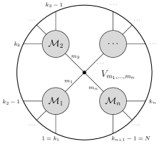
Figure 8: $N$-point diagram $\mathcal{M}_{N}$ with $n$-point vertex $V_{m_{1},\dots,m_{n}}$.

In order to investigate how the vanishing condition of $\mathcal{M}_{N}$ is related to $\mathcal{M}^{(m)}_{n\text{-contact}}$, we will factorize out $\mathcal{M}_{1},\dots,\mathcal{M}_{n}$ successively and look into the remaining (shifted) $n$-point contact diagram. Throughout this process we always consider the case that the descendant level of the propagator connecting the $n$-point vertex and $\mathcal{M}_{n}$ (denoted by $m^{\prime}$ temporarily) is minimized, since at the final step we will find that $\mathcal{M}_{N}\neq 0$ only if $\mathcal{M}^{\mathchoice{\raisebox{-3.0pt}{$\displaystyle(m^{\prime})$}}{\raisebox{-3.0pt}{$\textstyle(m^{\prime})$}}{\raisebox{-3.0pt}{$\scriptstyle(m^{\prime})$}}{\raisebox{-3.0pt}{$\scriptscriptstyle(m^{\prime})$}}}_{n\text{-contact}}\neq 0$. Thus in order to make $\mathcal{M}_{N}\neq 0$, we should strive to minimize $m^{\prime}$ to be less than $m_{0}$.

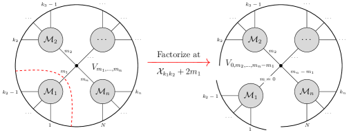
Figure 9: Factorize out $\mathcal{M}_{1}$.

First let us factorize out $\mathcal{M}_{1}$, as shown in Figure 9. According to assumption (77), the half amplitude containing the $n$-point vertex is a linear combination of amplitudes with descendant levels of propagators raised by at most $\sum n_{ab}\leqslant m_{1}$, which reads

$$\mathcal{M}^{(m_{1})}_{Ik_{2}\cdots N}=\sum_{\begin{subarray}{c}\sum n_{ab}\leqslant m_{1}\\ \ldots\end{subarray}}\mathcal{M}_{Ik_{2}\cdots N}(\delta_{ab}+n_{ab})\times\cdots.$$

It would be helpful to imagine that $\sum n_{ab}=m$ are distributed to $\delta_{ab}$, raising them to $\delta_{ab}+n_{ab}$, ascending the descendant levels of some propagators in $\mathcal{M}_{Ik_{2}\cdots N}$. In order to minimize $m^{\prime}$, we should have all the nonzero $n_{ab}$ distributed to $\delta_{ab}\in\mathcal{X}_{k_{n}k_{n+1}}$, raising the descendant level of $\mathcal{X}_{k_{n}k_{n+1}}$ from $m_{n}-m_{1}$ to $m_{n}$. In other words, some terms in $\mathcal{M}_{Ik_{2}\cdots N}$ with $m^{\prime}\geqslant m_{n}-m_{1}$ must exist, otherwise the descendant level of $\mathcal{X}_{k_{n}k_{n+1}}$ in $\mathcal{M}^{\mathchoice{\raisebox{-3.0pt}{$\displaystyle(m_{1})$}}{\raisebox{-3.0pt}{$\textstyle(m_{1})$}}{\raisebox{-3.0pt}{$\scriptstyle(m_{1})$}}{\raisebox{-3.0pt}{$\scriptscriptstyle(m_{1})$}}}_{Ik_{2}\cdots N}$ and $\mathcal{M}_{N}$ would be less than $m_{n}$.

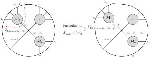
Figure 10: Factorize out $\mathcal{M}_{2}$.

Labelling the external leg $I$ from factorization by $\color[rgb]{0,0,1}1$ highlighted in blue, we move on to factorizing out $\mathcal{M}_{2}$, as shown in Figure 10, and sequentially $\mathcal{M}_{3},\dots,\mathcal{M}_{n-1}$. Similar argument shows that some terms in $\mathcal{M}_{{\color[rgb]{0,0,1}1\cdots n-1}k_{n}\cdots N}$ (left side of Figure 11) with $m^{\prime}\geqslant m_{\flat}$ must exist, otherwise the descendant level of $\mathcal{X}_{k_{n}k_{n+1}}$ in $\mathcal{M}_{N}$ can not be as large as $m_{n}$.

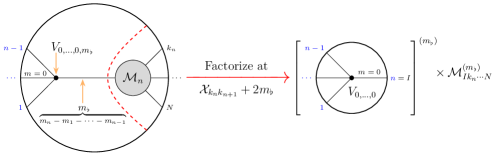
Figure 11: Factorize out $\mathcal{M}_{n}$ to get $\mathcal{M}^{(m_{\flat})}_{n\text{-contact}}$.

At the last step, we factorize out $\mathcal{M}_{n}$ from $\mathcal{M}_{{\color[rgb]{0,0,1}1\cdots n-1}k_{n}\cdots N}$, as shown in Figure 11, where the external legs $\color[rgb]{0,0,1}1,\dots,n-1$ highlighted in blue are the legs coming from factorization. As stated before, the minimal $m^{\prime}$ to have non-vanishing $\mathcal{M}_{N}$ is $m_{\flat}=m_{n}-m_{1}-\cdots-m_{n-1}$. Now from the factorization at $\mathcal{X}_{k_{1}k_{n}}$ we see that, the minimal $m$ by which $\mathcal{M}_{n\text{-contact}}$ need to be shifted is exactly $m_{\flat}$. In other words, all the terms in $\mathcal{M}_{{\color[rgb]{0,0,1}1\cdots n-1}k_{n}\cdots N}$ come from some shifted amplitudes $\mathcal{M}^{{\mathchoice{\raisebox{-3.0pt}{$\displaystyle(m^{\prime})$}}{\raisebox{-3.0pt}{$\textstyle(m^{\prime})$}}{\raisebox{-3.0pt}{$\scriptstyle(m^{\prime})$}}{\raisebox{-3.0pt}{$\scriptscriptstyle(m^{\prime})$}}}}_{n\text{-contact}}$ with $m^{\prime}\geqslant m_{\flat}$. Thus if $\mathcal{M}^{\mathchoice{\raisebox{-3.0pt}{$\displaystyle(m)$}}{\raisebox{-3.0pt}{$\textstyle(m)$}}{\raisebox{-3.0pt}{$\scriptstyle(m)$}}{\raisebox{-3.0pt}{$\scriptscriptstyle(m)$}}}_{n\text{-contact}}$ vanishes for all $m\geqslant m_{0}$ and $m_{\flat}\geqslant m_{0}$, then all the terms in $\mathcal{M}_{N}$ would contain a vanishing shifted $n$-point contact diagram, hence $\mathcal{M}_{N}$ must vanish. This completes the proof. ∎

Then we can apply Lemma 5.2 to the supergluon amplitudes containing only 3- and 4-point vertices in form of $V_{m_{1},m_{2},m_{3}}$ and $V_{m_{1},m_{2},m_{3},m_{4}}$. Without lost of generality, assuming $m_{1}\leqslant\cdots\leqslant m_{n}$, we have the following vertices existence conditions

• $3$-point vertices must have $m_{1}+m_{2}\geqslant m_{3}$.

• $4$-point vertices must have $m_{1}+m_{2}+m_{3}+1\geqslant m_{4}$.

Now let us move on to the final step, and investigate how the descendant levels can be restricted by the above vertices existence conditions. With careful observation, we find a helpful property of tree Witten sub-diagram with only 3- and 4-point vertices that, if the descendant levels of propagators connected to it are given by $m_{1},m_{2},\dots,m_{n}$, as shown in Figure 13, then the maximal possible value of $m_{n}$ is given by

$$m_{\text{max}}=m_{1}+m_{2}+\cdots+m_{n-1}+(\text{number of 4-point vertex in }\mathcal{M})$$ (78)

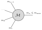
Figure 12: Witten sub-diagram.

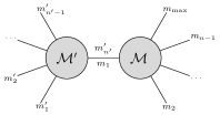
Figure 13: Induction of sub-diagram.

This can be proved by induction. Obviously (78) holds for sub-diagrams with a single vertex. Now suppose that (78) holds for two tree sub-diagrams $\mathcal{M}$ and $\mathcal{M}^{\prime}$, then for the sub-diagram $\mathcal{M}^{\prime}+\mathcal{M}$ constructed by connecting $\mathcal{M}^{\prime}$ to $\mathcal{M}$ as in Figure 13, we have

$$m^{\mathcal{M}^{\prime}+\mathcal{M}}_{\text{max}} =m^{\mathcal{M}^{\prime}}_{\text{max}}+m_{2}+\cdots+m_{n-1}+(\text{number of 4-point vertex in }\mathcal{M})$$ (79)

$$=m^{\prime}_{1}+m^{\prime}_{2}+\cdots+m^{\prime}_{n^{\prime}-1}+m_{2}+\cdots+m_{n-1}$$

$$\phantom{=m^{\prime}_{1}}\;+(\text{number of 4-point vertex in }\mathcal{M}^{\prime}+\mathcal{M})$$

Now we are just one step away from the desired Conjecture 5.1. Note that for the cut $\mathcal{X}_{ij}$ of a Witten diagram $\mathcal{M}$, the maximal number of 4-point vertices in $\mathcal{M}$ is exactly $\lfloor\frac{||i-j||-1}{2}\rfloor$, we draw the conclusion that the poles of $\mathcal{X}_{ij}$ must truncate at $\lfloor\frac{||i-j||+1}{2}\rfloor$.

5.2 Feynman rules for single-trace amplitudes

Using the algorithm described in section 3, we have explicitly computed supergluon amplitudes up to $n=8$, as well as the single-trace part of $\mathcal{M}_{\leq 12}^{(s)}$ and $\mathcal{M}_{\leq 9}^{(v)}$. Interestingly, the results closely resemble the flat-space amplitudes obtained through simple Feynman rules.

For the single-trace part $M_{n}^{(s)}(\rm ST)\equiv M_{n}^{(s)}(12\cdots n)$ and $M_{n}^{(v)}(\rm ST)\equiv M_{n}^{(v)}(12\cdots(n-1))$, we are able to make the intuition precise. It turns out that these partial amplitudes can be viewed as arising from the following bulk interaction:

$$\mathcal{L}_{\text{int, color-ordered}}\supset g\phi^{3}-2g^{2}\phi^{4}+\lambda A^{\bar{\mu}}\phi\overleftrightarrow{\nabla}_{\bar{\mu}}\phi.$$ (80)

One can try to write down all Witten diagrams needed to compute $\mathcal{M}_{n}^{(s)}(12\cdots n)$ and $\mathcal{M}_{n}^{(v)}(12\cdots(n-1))$, and then compute their individual contribution to the Mellin amplitude following the Mellin space Feynman rules. The rules for scalar interactions $\phi^{3}$ and $\phi^{4}$ were derived in Paulos:2011ie ; Nandan:2011wc . On the other hand, the rules for $A^{\bar{\mu}}\phi\overleftrightarrow{\nabla}_{\bar{\mu}}\phi$ were not previously known; we will derive the rules following their strategy in the appendix. Here, we merely list the resulting Feynman rules. For a given Witten diagram,

• Associate auxiliary momenta to each propagator such that momentum is conserved at each vertex. The momentum $p_{i}$ of a bulk-to-boundary propagator satisfies $-p_{i}^{2}=\tau_{i}$, the conformal twist $\Delta_{i}-J_{i}$ of the $i$-th operator. Lorentz products of auxiliary momenta are related to Mellin variables through $\delta_{ij}=p_{i}\cdot p_{j}$.

• To every propagator with auxiliary momentum $p$ corresponding to the exchange of an operator with twist $\tau$, assign a non-negative integer (descendant level) $m$. Bulk-to-boundary propagators have descendant level 0. Each propagator contributes

  $$\frac{-2}{m!\Gamma(\tau+m+1-h)}\frac{1}{(-p^{2}-\tau)-2m}.$$

• Every $\phi^{k}$ vertex joining $k$ scalar propagators with descendant levels $m_{1},\dots,m_{k}$ contributes Paulos:2011ie

  $$V^{\Delta_{1},\dots,\Delta_{k}}_{m_{1},\dots,m_{k}} =\sum_{n_{1}=0}^{m_{1}}\dots\sum_{n_{k}=0}^{m_{k}}\Gamma\!\left[\frac{\Sigma\Delta-d}{2}+{\textstyle\sum_{i}n_{i}}\right]\prod_{i=1}^{k}\frac{(-m_{i})_{n_{i}}}{n_{i}!(1-h+\Delta_{i})_{n_{i}-m_{i}}}$$

• Every $A^{\bar{\mu}}\phi\overleftrightarrow{\nabla}_{\bar{\mu}}\phi$ vertex joining scalar propagators with descendant levels $m_{L},m_{R}$ and a vector bulk-to-boundary propagator contributes

  $$V^{\Delta_{L},\Delta_{R},\Delta_{v}+1}_{m_{L},m_{R},0}\times\left[\texttt{zp[$L$]}\left(\frac{m_{R}-m_{L}}{2}+\frac{\Delta_{v}-1}{4}\right)-\texttt{zp[$R$]}\left(\frac{m_{L}-m_{R}}{2}+\frac{\Delta_{v}-1}{4}\right)\right],$$

  where $L,R$ are the total inflow of auxiliary momenta from the left and right.

• Sum over all possible assignments of descendant levels associated with bulk-to-bulk propagators.

Let us be more concrete. For instance, consider the following terms in $M_{8}^{(s)}({\rm ST})$:

$$M_{8}^{(s)}({\rm ST})=\frac{-32}{\mathcal{X}_{14}\mathcal{X}_{16}}+\frac{-32}{\mathcal{X}_{14}(\mathcal{X}_{16}-2)}+\frac{-96}{(\mathcal{X}_{14}-2)(\mathcal{X}_{16}-2)}+\frac{-32}{\mathcal{X}_{13}\mathcal{X}_{14}\mathcal{X}_{16}\mathcal{X}_{17}}+\cdots$$

We can draw their corresponding Witten diagrams (with descendant-level assignments) as follows:

$$\begin{array}[]{cccc}\includegraphics[width=86.72267pt]{newimages/8s_1.pdf}&\includegraphics[width=86.72267pt]{newimages/8s_2.pdf}&\includegraphics[width=86.72267pt]{newimages/8s_3.pdf}&\includegraphics[width=86.72267pt]{newimages/8s_4.pdf}\\ \downarrow&\downarrow&\downarrow&\downarrow\\ -32&-32&-96&-32\end{array}$$

Using the Feynman rules described above, we indeed obtain the correct coefficient. For example, consider the third diagram above:

$$\frac{-2}{(0!)^{2}}\frac{-2}{(0!)^{2}}(-2)^{3}V^{2222}_{0001}V^{2222}_{0011}V^{2222}_{0001}=-96.$$

We can similarly check the following diagram-coefficient pair for higher-point single-trace amplitudes:

$$\to\frac{(-2)^{7}}{(1!)^{2}(2!)^{2}(1!)^{2}}V^{2222}_{0001}V^{2222}_{0012}V^{2222}_{0012}V^{2222}_{0001}=-512,$$

$$\to\frac{(-2)^{8}}{(1!)^{2}(2!)^{2}(2!)^{2}(1!)^{2}}V^{2222}_{0001}V^{2222}_{0012}V^{222}_{022}V^{2222}_{0012}V^{2222}_{0001}=1024,$$

$$\to\frac{(-2)^{8}}{(1!)^{2}(1!)^{2}(1!)^{2}(2!)^{2}}V^{2222}_{0001}V^{2222}_{0012}V^{222}_{112}V^{2222}_{0001}V^{2222}_{0001}=1024,$$

$$\to\frac{(-2)^{8}}{(1!)^{2}(1!)^{2}(1!)^{2}(1!)^{2}}(V^{2222}_{0001})^{3}V^{2222}_{0111}V^{222}_{011}=2816,$$

$$\to\frac{(-2)^{9}}{(1!)^{6}(2!)^{2}}(V^{2222}_{0001})^{3}V^{2222}_{0112}V^{2222}_{0012}=-14336,$$

$$\to\frac{(-2)^{9}}{(1!)^{8}}(V^{2222}_{0001})^{4}V^{2222}_{1111}=-27136.$$

For the single-gluon amplitude $M_{5}^{(v)}({\rm ST})$,

$$M_{5}^{(v)}({\rm ST}) =\frac{2(\texttt{zp[$123$]}-\texttt{zp[$4$]})}{\mathcal{X}_{14}}+\frac{2(\texttt{zp[$1$]}-\texttt{zp[$234$]})}{\mathcal{X}_{25}}+\frac{-4\texttt{zp[$4$]}}{\mathcal{X}_{14}-2}+\frac{4\texttt{zp[$1$]}}{\mathcal{X}_{25}-2}$$

$$+\frac{2(\texttt{zp[$12$]}-\texttt{zp[$34$]})}{\mathcal{X}_{13}\mathcal{X}_{35}}+\frac{2(\texttt{zp[$123$]}-\texttt{zp[$4$]})}{\mathcal{X}_{14}\mathcal{X}_{24}}+\cdots$$

Figure 14: A typical diagram contributing to $M_{5}^{(v)}({\rm ST})$.

Consider the diagram Figure 14. The propagator yields a factor of $\frac{-2}{(0!)^{2}}=-2$, while the $\phi^{4}$ vertex gives $-2V^{2222}_{0000}=-2$. For the gluon vertex, to its left we have total momentum inflow $p_{1}+p_{2}+p_{3}$, so that $\texttt{zp[$L$]}=\texttt{zp[$123$]}$ and $\texttt{zp[$R$]}=\texttt{zp[$4$]}$. Using the Feynman rule described earlier, it gives $V^{224}_{000}=\frac{\texttt{zp[$123$]}-\texttt{zp[$4$]}}{2}$ (omitting the overall $i\sqrt{2/3}$ normalization). Putting everything together, we see that this diagram contributes $\frac{2(\texttt{zp[$123$]}-\texttt{zp[$4$]})}{\mathcal{X}_{14}}$. For another term, $\frac{-4\texttt{zp[$4$]}}{\mathcal{X}_{14}-2}$, we have $(m_{L},m_{R})=(1,0)$ so that only the $\texttt{zp[$L$]}=\texttt{zp[$123$]}$ term have vanishing prefactor. One can similarly check that the Feynman rules give the correct prefactor for all other terms as well.

Some higher-point diagrams contributing to $M_{n}^{(v)}({\rm ST})$ are:

$$\begin{array}[]{ccc}\includegraphics[width=86.72267pt,align=c]{newimages/7v_1.pdf}&\includegraphics[width=86.72267pt,align=c]{newimages/7v_2.pdf}&\includegraphics[width=86.72267pt,align=c]{newimages/7v_3.pdf}\\ \downarrow&\downarrow&\downarrow\\ 24(\texttt{zp[$123$]}-\texttt{zp[$456$]})&16\texttt{zp[$123$]}&-16\texttt{zp[$1$]}\\ \\ \hline\cr\\ \includegraphics[width=86.72267pt,align=c]{newimages/9v_1.pdf}&\includegraphics[width=86.72267pt,align=c]{newimages/9v_2.pdf}\\ \downarrow&\downarrow\\ 0&256\texttt{zp[$123$]}\end{array}$$

5.3 Universal behavior analogous to collinear and soft limits

Scattering amplitudes of massless particles in flat space exhibit two well-known universal behaviours, namely factorizations under collinear and soft limits. In this subsection we show that AdS supergluon amplitudes and spinning amplitudes have similar behavior despite that we do not have “massless particles” here.

Recall that in the collinear limit, i.e. two particles become collinear ($s_{ij}=(p_{i}+p_{j})^{2}\to 0$), the $n$-point scattering amplitude factorizes into $(n{-}1)$-point amplitude and a universal factor called splitting factor, while in the soft limit, i.e. the momentum of a particle become soft ($p_{i}\to 0$), the $n$-point scattering amplitude also factorizes into $(n{-}1)$-point amplitude and a universal factor called soft factor. The collinear/soft behaviours origin from singularities of the scattering amplitudes in the flat space (c.f. Dixon:1996wi ).

In AdS space, the singularities of scattering amplitudes arise from the Operator Product Expansion(OPE) limit, i.e. the position of two particles becomes close $x_{i,j}^{2}=(x_{i}-x_{j})^{2}\to 0$. The OPE limit is similar to the collinear limit. In the Mellin representation of AdS amplitude, the leading twist contribution to the OPE limit ($x_{1}\to x_{2}$) corresponds to the Mellin variable $\mathcal{X}_{1,3}\to 0$, leading to factorization of the Mellin amplitude. For $n$-point supergluon Mellin amplitude, when $\mathcal{X}_{1,3}\to 0$, the factorization of Mellin amplitude gives

$$\mathop{\rm Res}_{\mathcal{X}_{13}=0}\mathcal{M}_{n}^{(s)}=\mathcal{N}_{s}\leavevmode\nobreak\ \texttt{glueR}\left(\mathcal{M}_{12I}^{(s)}\mathcal{M}_{3\cdots nI}^{(s)}\right)+\mathcal{N}_{v}\sum_{a=1}^{2}\sum_{i=3}^{n}\delta_{ai}\mathcal{M}_{12I}^{(v)a}\mathcal{M}_{3\cdots nI}^{(v)i}\,,$$ (81)

where the residue of the Mellin amplitude at $\mathcal{X}_{13}=0$ has two contributions: scalar exchange and gluon exchange. To distinguish between these two exchanges, we consider a limit for identifying the SU$(2)_{R}$ spinors $v_{1}$ and $v_{2}$ as $v_{I}$, then $v_{1}\cdot v_{2}=\langle 12\rangle\to v_{I}^{2}=0$. In this limit, only the incompatible R-structure (i.e., scalar exchange) proportional to $\langle 12\rangle$ but not $\langle 12\rangle^{2}$ contributes to the leading order. In this way we obtain the “leading collinear limit” for supergluon amplitudes analogous to collinear limit in the flat space.

$$\mathcal{M}_{n}^{(s)}\xrightarrow[\mathcal{X}_{13}\to 0]{\langle 12\rangle\to 0}\leavevmode\nobreak\ \mathcal{N}_{s}\leavevmode\nobreak\ \frac{\langle 12\rangle}{\mathcal{X}_{13}}\times\mathcal{M}_{3\cdots nI}^{(s)}\,,$$ (82)

where the $n$-point supergluon amplitude $\mathcal{M}_{n}^{(s)}$ factorizes into the $(n{-}1)$-point supergluon amplitude $\mathcal{M}_{3\cdots nI}^{(s)}$ and the “splitting factor” $\mathcal{N}_{s}\frac{\langle 12\rangle}{\mathcal{X}_{13}}$ for supergluon amplitudes. Compared with the color-ordered scalar amplitude with Tr$(\phi^{3})$ interaction in the flat space, the amplitude factors in the collinear limit, $s_{12}\to 0$,

$$\mathcal{A}_{n}^{\phi^{3}}(1,\ldots,n)\xrightarrow[s_{12}\to 0]{}\frac{1}{s_{12}}\mathcal{A}_{n{-}1}^{\phi^{3}}(3\cdots nI)\,,$$ (83)

where $\mathcal{A}_{n}^{\phi^{3}}(1,\ldots,n)$ denotes the $n$-point Tr$(\phi^{3})$ tree-level amplitude in the color ordering of $(1,\ldots,n)$.

The derivation for soft limit is very similar. In flat space the soft singularity arises from all poles of the form $s_{i,n}$ when $p_{n}\to 0$. For color-ordered amplitudes, only $s_{n{-}1,n}$ and $s_{1,n}$ contribute. The “leading soft ” limit of supergluon amplitude in AdS, arises from the limit of $\mathcal{X}_{1(n{-}1)}/\mathcal{X}_{2n}\to 0$ with identifying $\mathcal{X}_{jn}$ and $\mathcal{X}_{1j}$ for any $j$. Similar to collinear limit, we need to take an operator for the SU$(2)_{R}$ spinors $v_{n}$, specifically any $V_{\cdots n}\to V_{\cdots}$, in order to suppress the contribution from gluon exchange. In the gluon exchange, the R-structures of $M_{(n{-}1)nI}^{(v)a}/M_{1nI}^{(v)a}$ always vanish ($V_{(n{-}1)n}/V_{1n}\to V_{n{-}1}/V_{1}=0$). The second terms from the glueR of scalar exchange also vanish for the same reason:

$$\mathcal{M}_{n}^{(s)}\xrightarrow[\mathcal{X}_{1(n{-}1)}/\mathcal{X}_{2n}\to 0]{V_{\cdots n}\to V_{\cdots}}\mathcal{N}_{s}\frac{1}{\mathcal{X}_{1(n{-}1)}}\mathcal{M}_{1\cdots(n{-}1)}^{(s)}+\mathcal{N}_{s}\frac{1}{\mathcal{X}_{2n}}\mathcal{M}_{2\cdots n}^{(s)}=\mathcal{N}_{s}\left(\frac{1}{\mathcal{X}_{1(n{-}1)}}+\frac{1}{\mathcal{X}_{2n}}\right)\mathcal{M}_{1\cdots(n{-}1)}^{(s)}\,,$$ (84)

where in the second equality, we identify $\mathcal{X}_{jn}$ and $\mathcal{X}_{1j}$. In the “leading soft limit”, the $n$-point supergluon amplitude $\mathcal{M}_{n}^{(s)}$ factorizes into $(n{-}1)$-point supergluon amplitude $\mathcal{M}_{1\cdots(n{-}1)}^{(s)}$ and the “soft factor” $\mathcal{N}_{s}\left(\frac{1}{\mathcal{X}_{1(n{-}1)}}+\frac{1}{\mathcal{X}_{2n}}\right)$ for supergluon amplitudes. This can be compared with the color-ordered scalar amplitude with Tr$(\phi^{3})$ interaction in the flat space:

$$\mathcal{A}_{n}^{\phi^{3}}(1,\ldots,n)\xrightarrow[s_{n{-}1,n}\to 0]{s_{1n}\to 0}(\frac{1}{s_{n{-}1,n}}+\frac{1}{s_{1n}})\mathcal{A}_{n{-}1}^{\phi^{3}}(1\cdots(n{-}1))\,.$$ (85)

Very nicely, similar arguments can be applied for the spinning amplitudes. For collinear limit,

$$\mathop{\rm Res}_{\mathcal{X}_{1(n-{1})}=0}\mathcal{M}_{n}^{(v)}=\mathcal{N}_{s}\texttt{glueR}\left(\mathcal{M}_{12\cdots(n{-}2)I}^{(s)}\mathcal{M}_{I(n{-}1)n}^{(v)}\right)\,,$$ (86)

where the glueR (21) is simplified, because the R-structure of $\mathcal{M}_{I(n{-}1)n}^{(v)}$ is $V_{I(n{-}1)}$. After the glueR, the R-structure of $\mathcal{M}_{12\cdots(n{-}2)I}^{(s)}$ becomes the same R-structure of $\mathcal{M}_{12\cdots(n{-}2)(n{-}1)}^{(s)}$.

$$\mathcal{M}_{n}^{(v)}\xrightarrow[\mathcal{X}_{1(n{-}1)}\to 0]{}\tilde{\mathcal{N}}_{s}\frac{\texttt{zp[$n{-}1$]}-\texttt{zp[$12\cdots n{-}2$]}}{\mathcal{X}_{1(n{-}1)}}\mathcal{M}_{12\cdots(n{-}2)I}^{(s)}\,,$$ (87)

where $\tilde{\mathcal{N}}_{s}$ absorbs the overall factor from the 3-point spinning amplitude, $\tilde{\mathcal{N}}_{s}=\mathcal{N}_{s}\frac{i\sqrt{2/3}}{2}$. The $n$-point spinning amplitude $\mathcal{M}_{n}^{(v)}$ factorizes into $(n{-}1)$-point supergluon amplitude $\mathcal{M}_{12\cdots(n{-}2)I}^{(s)}$ and the “splitting factor” $\tilde{\mathcal{N}}_{s}\frac{\texttt{zp[$n{-}1$]}-\texttt{zp[$12\cdots n{-}2$]}}{\mathcal{X}_{1(n{-}1)}}$ for spinning amplitudes. Compared with the color-ordered scalar amplitude minimal coupled with one gluon in the flat space, the amplitude factors in the collinear limit, $s_{(n{-}1)n}\to 0$,

$$\mathcal{A}_{n}^{{\rm YM}+\phi^{3}}(1,\ldots,n{-}1;n)\xrightarrow[s_{(n{-}1)n}\to 0]{}\frac{\epsilon_{n}\cdot p_{n{-}1}-\epsilon_{n}\cdot p_{12\ldots n{-}2}}{s_{(n{-}1)n}}\mathcal{A}_{n{-}1}^{\phi^{3}}(12\cdots(n{-}2)I)\,,$$ (88)

where $\mathcal{A}_{n}^{{\rm YM}+\phi^{3}}(1,\ldots,n{-}1;n)$ denotes the $n$-point tree-level amplitude with the $n-1$ scalar in the color ordering $(1,\ldots,n{-}1)$ and one gluon with the polarization vector $\epsilon_{n}$, and here the $p_{12\ldots n{-}2}=\sum_{i=1}^{n{-}2}p_{i}$.

The soft limit of the spinning amplitudes can be similarly derived as,

$$\mathcal{M}_{n}^{(v)}\xrightarrow[\mathcal{X}_{1(n{-}1)}\to 0]{\mathcal{X}_{2n}\to 0}\tilde{\mathcal{N}}_{s}\frac{\texttt{zp[$n{-}1$]}-\texttt{zp[$12\cdots n{-}2$]}}{\mathcal{X}_{1(n{-}1)}}\mathcal{M}_{12\cdots(n{-}1)}^{(s)}+\tilde{\mathcal{N}}_{s}\frac{\texttt{zp[$2\cdots n{-}1$]}-\texttt{zp[$1$]}}{\mathcal{X}_{2n}}\mathcal{M}_{2\cdots n}^{(s)}$$ (89)

$$=\tilde{\mathcal{N}}_{s}\left(\frac{\texttt{zp[$n{-}1$]}-\texttt{zp[$12\cdots n{-}2$]}}{\mathcal{X}_{1(n{-}1)}}+\frac{\texttt{zp[$2\cdots n{-}1$]}-\texttt{zp[$1$]}}{\mathcal{X}_{2n}}\right)\mathcal{M}_{1\cdots n{-}1}^{(s)}\,,$$

where in the second equality, we identify $\mathcal{X}_{jn}$ and $\mathcal{X}_{1j}$. In the “leading soft” limit, the $n$-point spinning amplitude $\mathcal{M}_{n}^{(v)}$ factorizes into $(n{-}1)$-point supergluon amplitude $\mathcal{M}_{1\cdots(n{-}1)}^{(s)}$ and the “soft factor” $\tilde{\mathcal{N}}_{s}\left(\frac{\texttt{zp[$n{-}1$]}-\texttt{zp[$12\cdots n{-}2$]}}{\mathcal{X}_{1(n{-}1)}}+\frac{\texttt{zp[$2\cdots n{-}1$]}-\texttt{zp[$1$]}}{\mathcal{X}_{2n}}\right)$ for spinning amplitudes. Compared with the color-ordered scalar amplitude minimal coupled with one gluon in the flat space, the amplitude factors in the soft limit, $p_{n}\to 0$, which equal to the $s_{1,n}\to 0,s_{(n{-}1)n}\to 0$ in this color ordering,

$$\mathcal{A}_{n}^{{\rm YM}+\phi^{3}}\xrightarrow[s_{(n{-}1)n}\to 0]{s_{1n}\to 0}\left(\frac{\epsilon_{n}\cdot p_{n{-}1}-\epsilon_{n}\cdot p_{12\ldots n{-}2}}{s_{(n{-}1)n}}+\frac{\epsilon_{n}\cdot p_{2\ldots n{-}1}-\epsilon_{n}\cdot p_{1}}{s_{1n}}\right)\mathcal{A}_{n{-}1}^{\phi^{3}}(12\cdots(n{-}1))\,.$$ (90)

6 Conclusions and Outlook

In this paper we have elaborated on a new, recursive method proposed in Cao:2023cwa for computing the holographic correlator of $n$ half-BPS operators with conformal dimension $\Delta=2$, or equivalently the $n$-point supergluon amplitudes in AdS${}_{5}\times S^{3}$ at tree level. By extracting $(n{-}1)$-point spinning amplitudes from the $n$-point supergluon one, in sec. 3 we have shown that these lower-point amplitudes suffice to determine the $(n{+}2)$-point supergluon amplitude from various factorizations and flat-space limit. This amounts to an improved proof for the constructibility of supergluon amplitudes to all multiplicities, which then immediately implies constructibility of spinning amplitudes as a byproduct.

Apart from providing valuable data for the study of AdS${}_{5}/$ CFT₄ holography, it is advantageous to have these beautiful expressions of $n$-point Mellin amplitudes (with a given color-ordering, expanded in a basis of R-symmetry structures Cao:2023cwa ), which provide an ideal playground for studying hidden structures of AdS amplitudes. One can view our results as the simplest generalizations of the flat-space “scalar-scaffolded” gluon amplitudes Arkani-Hamed:2023jry to AdS background. In addition to presenting explicit results in sec. 4, we have revealed several interesting new structures to all $n$. Most importantly, we have argued that the general structure of descendant poles satisfy the “half-circle rule” (see 5.1). For the single-trace case which we have computed to all $n$, we have derived remarkably simple “Feynman rules”: for supergluon case they are given by $\phi^{3}+\phi^{4}$ and for spinning case with additional interactions of gluon with 2 $\phi$s (see app. B for more details); we have also shown the analogy of collinear and soft limits for AdS amplitudes.

Our work has opened up many new avenues for future investigations. First of all, within our setting of supergluon tree amplitudes in $AdS_{5}\times S^{3}$, there are very interesting questions one can pursue. Although we have proved constructibility for all $n$, it is still important to explicitly run our algorithm for higher points, i.e. for multi-trace amplitudes with $n\geq 10$, and in particular it would be highly desirable to develop recursion relations for accomplishing this, which already exist for single-trace amplitudes. Relatedly, it would be interesting to derive “Feynman rules” beyond single-trace cases (both for supergluon and spinning amplitudes), which may be connected with other methods for evaluating Witten diagrams in Mellin space Chu:2023kpe ; Chu:2023pea ; Li:2023azu ; Paulos:2011ie . On the other hand, an important conceptual problem is how to extract multi-gluon spinning amplitudes, since we have yet to develop a formalism with simple factorization properties Goncalves:2014rfa to treat such multi-spinning amplitudes in Mellin space nicely.

Another important direction is to study all these AdS amplitudes directly in position space, and to see if our program and even the recursion could be formulated there. For this purpose, one may consider the “differential representation” for these higher-point amplitudes in position space Huang:2024dck , where nice structures have been found in four-point AdS amplitudes in various settings. In particular, the $n=6$ amplitude involves Witten diagrams that evaluate to elliptic integrals Paulos:2011ie ; Paulos:2012nu , which certainly deserve further investigations.

Despite all these open questions, we emphasize that these supergluon amplitudes already provide a rich collection of data and insights for future study of holographic correlator and scattering amplitudes in AdS spacetime. As we have mentioned, it is advantageous to view our results as AdS generalizations of the flat-space program of scalar-scaffolded gluons proposed in Arkani-Hamed:2023jry . Given that the latter is based on combinatorial structures for surfaces Arkani-Hamed:2023mvg ; Arkani-Hamed:2023lbd , it is natural to ask if there exists a similar formulation for AdS supergluon amplitudes, and if one could connect it to the exciting progress on worldsheet formulation of AdS Veneziano amplitudes Alday:2024ksp (see also Alday:2023kfm ). A number of intriguing properties have been uncovered recently for scaffolded gluons in flat space, such as zeros and new factorizations or splitting behaviors Arkani-Hamed:2023swr ; Cachazo:2021wsz ; Cao:2024gln ; Arkani-Hamed:2023jry , and it would be fascinating to look for hints for such structures and properties in our AdS amplitudes.

Beyond the simplest supergluon amplitudes, it would be very interesting to study scattering of higher Kaluza-Klein modes, which would require some extensions regarding R-symmetry structures and factorization properties. Preliminary studies show that we can at least obtain five-point KK amplitudes in this way, and it is important to develop our method further for constructing higher-point KK amplitudes. Given recent progress on hidden symmetries for four-point (reduced) correlators Caron-Huot:2018kta ; Rastelli:2019gtj ; Alday:2021odx ; Abl:2021mxo ; Rigatos:2024yjo , it would be highly desirable to see if such hidden symmetries could be extended to higher points and provide a “generating function” of KK amplitudes. Another motivation is that the observed double-copy relation Zhou:2021gnu relates supergluon amplitudes to supergraviton amplitudes as well as conformal scalar amplitudes which can serve as nice toy models. At least for conformal scalars such as $\phi^{3}$ in ${\rm AdS}_{d+1}\times S^{5-d}$, a version of “hidden symmetry” trivially holds.

It would also be extremely interesting to see how this entire program can be extended to supergravity amplitudes in $AdS_{5}\times S^{5}$, and especially for higher-point and/or spinning amplitudes. We remark that at least the flat-space limit for such supergravity amplitudes are known: for even points, they are given by generalization of scalar-scaffolded GR which turn out to be pion scattering amplitudes with interactions with gravity; these amplitudes are related to the YMS amplitudes by double copy Kawai:1985xq ; Bern:2008qj and can be computed again via nice CHY formulas Cachazo:2014xea . It would be fascinating to explore both these flat-space amplitudes and their AdS counterpart in the future.

Appendix A Coefficients of single-trace Witten diagrams

Let us summarize some coefficients of single-trace Witten diagrams up to $n=12$ for supergluon amplitudes, both as a check for the Feynman rules and to illustrate how non-trivial these amplitudes become for higher $n$.

Coefficient $=1$

Table 1: Coefficients of Witten diagrams contributing to $M_{6}^{(s)}({\rm ST})/(-2)^{3}$.

Coefficient $=1$

Table 2: Coefficients of Witten diagrams contributing to $M_{7}^{(s)}({\rm ST})/(-2)^{4}$.

Coefficient $=1$

Coefficient $=3$

Table 3: Coefficients of Witten diagrams contributing to $M_{8}^{(s)}({\rm ST})/(-2)^{5}$.

Coefficient $=1$

Coefficient $=2$

Coefficient $=3$

Table 4: Coefficients of Witten diagrams contributing to $M_{9}^{(s)}({\rm ST})/(-2)^{6}$.

Coefficient $=1$

Coefficient $=2$

Coefficient $=3$

Coefficient $=4$

Coefficient $=9$

Coefficient $=11$

Table 5: Coefficients of Witten diagrams contributing to $M_{10}^{(s)}({\rm ST})/(-2)^{7}$.

Coefficient $=1,3$

$\cdots$

Coefficient $=2$

Coefficient $=4$

Coefficient $=6$

Coefficient $=9$

Coefficient $=11$

Table 6: Coefficients of Witten diagrams contributing to $M_{11}^{(s)}({\rm ST})/(-2)^{8}$.

Coefficient $=1,2,3,4,6,9,11$

$\cdots$

Coefficient $=12$

Coefficient $=20$

Coefficient $=27$

Coefficient $=28$

Coefficient $=33$

Coefficient $=53$

Table 7: Coefficients of Witten diagrams contributing to $M_{12}^{(s)}({\rm ST})/(-2)^{9}$.

Coefficient $=2\texttt{zp[$L$]}$

Coefficient $=4\texttt{zp[$L$]}$

Coefficient $=6\texttt{zp[$L$]}$

Coefficient $=8\texttt{zp[$L$]}$

Coefficient $=18\texttt{zp[$L$]}$

Coefficient $=22\texttt{zp[$L$]}$

Continued on the next page

Table 8: Coefficients of Witten diagrams contributing to $M_{9}^{(v)}({\rm ST})/2^{5}$.

Continued from the previous page

Coefficient $=\texttt{zp[$L$]}-\texttt{zp[$R$]}$

Coefficient $=3(\texttt{zp[$L$]}-\texttt{zp[$R$]})$

Coefficient $=9(\texttt{zp[$L$]}-\texttt{zp[$R$]})$

Coefficient $\propto\texttt{zp[$R$]}$

$\cdots$

Table 9: Coefficients of Witten diagrams contributing to $M_{9}^{(v)}({\rm ST})/2^{5}$.

Appendix B Derivation of $A^{\bar{\mu}}\phi\overleftrightarrow{\nabla}_{\bar{\mu}}\phi$ Feynman rules

In this appendix, we derive the tree-level Mellin space Feynman rule of an on-shell vector and two possibly off-shell scalars. To be completely rigorous, we should follow Nandan:2011wc and show that such a Feynman rule exists and that we can write down an expression for each vertex or edge of a Witten diagram, regardless of the other parts of the diagram. However, we decide to take a short-cut by assuming the existence of Feynman rules. This way, we need only compute a specific Witten diagram (Fig. 15(a)) and extract the corresponding rules.

(a)

(b)

Figure 15: (a) A Witten diagram to extract the $A^{\bar{\mu}}\phi\overleftrightarrow{\nabla}_{\bar{\mu}}\phi$ vertex. (b) A scalar Witten diagram to compare the result. The dotted line indicates the integration over $Q\in\partial{\rm AdS}$ using the split representation (92).

Using the embedding space formalism, the scalar propagator reads

$$G^{\Delta}_{B\partial}(X,P) =\frac{1}{2\pi^{h}\Gamma(1+\Delta-h)}\int_{0}^{\infty}\frac{{\rm d}t}{t}t^{\Delta}e^{-2tX\cdot P},$$ (91)

$$G^{\delta}_{BB}(X_{1},X_{2}) =\int[{\rm d}c]f_{\delta}(c)\int_{\partial{\rm AdS}}{\rm d}Q\int_{0}^{\infty}\frac{{\rm d}s}{s}\frac{{\rm d}\bar{s}}{\bar{s}}s^{h+c}\bar{s}^{h-c}e^{-2Q\cdot(sX_{1}+\bar{s}X_{2})},$$ (92)

where

$$f_{\delta}(c)=\frac{1}{2\pi^{2h}}\frac{1}{((\delta-h)^{2}-c^{2})\Gamma(c)\Gamma(-c)}.$$ (93)

The gluon bulk-to-boundary propagator can be extracted from the scalar propagator using a differential operator:

$$D_{\Delta}^{MA}=\frac{\Delta-1}{\Delta}\eta^{MA}+\frac{1}{\Delta}\frac{\partial}{\partial P_{M}}P^{A},$$ (94)

$$E_{\Delta}^{MA}(X,P)=D_{\Delta}^{MA}G_{B\partial}^{\Delta}(X,P).$$ (95)

For the interaction vertex $A^{\bar{\mu}}\phi\overleftrightarrow{\nabla}_{\bar{\mu}}\phi$, the position space Feynman rules can be found in eq.(6.3) of Paulos:2011ie . From these building blocks, the above Witten diagram evaluates to (omitting overall constants)

$$G^{M} =D_{\Delta_{5}}^{MA}\int_{Q_{1},Q_{2},X_{1},X_{2},X_{3}}\frac{{\rm d}t_{1}}{t_{1}}t_{1}^{\Delta_{1}}\frac{{\rm d}t_{2}}{t_{2}}t_{2}^{\Delta_{2}}\frac{{\rm d}t_{3}}{t_{3}}t_{3}^{\Delta_{3}}\frac{{\rm d}t_{4}}{t_{4}}t_{4}^{\Delta_{4}}\frac{{\rm d}t_{5}}{t_{5}}t_{5}^{\Delta_{5}}[{\rm d}c_{1}][{\rm d}c_{2}]f_{\delta_{1}}(c_{1})f_{\delta_{2}}(c_{2})$$

$$\times\frac{{\rm d}s_{1}}{s_{1}}s_{1}^{h+c_{1}}\frac{{\rm d}\bar{s}_{1}}{\bar{s}_{1}}\bar{s}_{1}^{h-c_{1}}\frac{{\rm d}s_{2}}{s_{2}}s_{2}^{h+c_{2}}\frac{{\rm d}\bar{s}_{2}}{\bar{s}_{2}}\bar{s}_{2}^{h-c_{2}}(\bar{s}_{1}Q_{1,A}-\bar{s}_{2}Q_{2,A})$$

$$\times e^{-2X_{1}\cdot(t_{1}P_{1}+t_{2}P_{2}+s_{1}Q_{1})-2X_{3}\cdot(t_{3}P_{3}+t_{4}P_{4}+s_{2}Q_{2})-2X_{2}\cdot(t_{5}P_{5}+\bar{s}_{1}Q_{1}+\bar{s}_{2}Q_{2})}.$$

Without loss of generality, consider the $-\bar{s}_{2}Q_{2,A}$ term. Integrating away $X_{1},X_{2},X_{3}\in{\rm AdS}$ and $Q_{1},Q_{2}\in\partial{\rm AdS}$, we arrive at

$$G_{2}^{M} =D_{\Delta_{5}}^{MA}\int\frac{{\rm d}t_{1}}{t_{1}}t_{1}^{\Delta_{1}}\frac{{\rm d}t_{2}}{t_{2}}t_{2}^{\Delta_{2}}\frac{{\rm d}t_{3}}{t_{3}}t_{3}^{\Delta_{3}}\frac{{\rm d}t_{4}}{t_{4}}t_{4}^{\Delta_{4}}\frac{{\rm d}t_{5}}{t_{5}}t_{5}^{\Delta_{5}}[{\rm d}c_{1}][{\rm d}c_{2}]f_{\delta_{1}}(c_{1})f_{\delta_{2}}(c_{2})$$

$$\times\frac{{\rm d}s_{1}}{s_{1}}s_{1}^{h+c_{1}}\frac{{\rm d}\bar{s}_{1}}{\bar{s}_{1}}\bar{s}_{1}^{h-c_{1}}\frac{{\rm d}s_{2}}{s_{2}}s_{2}^{h+c_{2}}\frac{{\rm d}\bar{s}_{2}}{\bar{s}_{2}}\bar{s}_{2}^{h-c_{2}}$$

$$\times{\color[rgb]{0,0,1}-\bar{s}_{2}(s_{1}\bar{s}_{1}\bar{s}_{2}(t_{1}P_{1}+t_{2}P_{2})+s_{2}(t_{3}P_{3}+t_{4}P_{4})+\cancel{(1+\bar{s}_{1}^{2})\bar{s}_{2}t_{5}P_{5}})_{A}}$$

$$\times e^{-t_{1}t_{2}P_{12}-t_{3}t_{4}P_{34}+(s_{1}(t_{1}P_{1}+t_{2}P_{2})+\bar{s}_{1}t_{5}P_{5})^{2}+(s_{1}\bar{s}_{1}\bar{s}_{2}(t_{1}P_{1}+t_{2}P_{2})+s_{2}(t_{3}P_{3}+t_{4}P_{4})+(1+\bar{s}_{1}^{2})\bar{s}_{2}t_{5}P_{5})^{2}}$$

$$\times\Gamma\left(\frac{\Delta_{1}+\Delta_{2}+c_{1}-h}{2}\right)\Gamma\left(\frac{\Delta_{3}+\Delta_{4}+c_{2}-h}{2}\right)\Gamma\left(\frac{\Delta_{5}+1-c_{1}-c_{2}}{2}\right),$$

where we have used the notation $P_{ij}\equiv-2P_{i}\cdot P_{j}$. The term proportional to $P_{5A}$ can be dropped because it is annihilated by the differential operator in front. From the form of the exponential, we see that the blue factor can be written as a differential operator:

$${\color[rgb]{0,0,1}\text{blue}}=\frac{\bar{s}_{2}^{2}}{1+\bar{s}_{2}^{2}(1+\bar{s}_{1}^{2})}(P_{1,A}\partial_{P_{15}}+P_{2,A}\partial_{P_{25}})+\frac{1}{1+\bar{s}_{1}^{2}}(P_{3,A}\partial_{P_{35}}+P_{4,A}\partial_{P_{45}}).$$

Now, convert the $t$-integrals into Mellin representation using the Symanzik star formula.

$$G_{2}^{M} =D_{\Delta_{5}}^{MA}\int[{\rm d}c_{1}][{\rm d}c_{2}]f_{\delta_{1}}(c_{1})f_{\delta_{2}}(c_{2})[{\rm d}\gamma]\frac{{\rm d}s_{1}}{s_{1}}s_{1}^{h+c_{1}}\frac{{\rm d}\bar{s}_{1}}{\bar{s}_{1}}\bar{s}_{1}^{h-c_{1}}\frac{{\rm d}s_{2}}{s_{2}}s_{2}^{h+c_{2}}\frac{{\rm d}\bar{s}_{2}}{\bar{s}_{2}}\bar{s}_{2}^{h-c_{2}}(s_{1}\bar{s}_{1})^{-s_{12}}(s_{2}\bar{s}_{2})^{-s_{34}}$$

$$\times\left[\frac{\bar{s}_{2}^{2}}{1+\bar{s}_{2}^{2}(1+\bar{s}_{1}^{2})}(P_{1,A}\partial_{P_{15}}+P_{2,A}\partial_{P_{25}})+\frac{1}{1+\bar{s}_{1}^{2}}(P_{3,A}\partial_{P_{35}}+P_{4,A}\partial_{P_{45}})\right]\prod_{i<j}[P_{ij}]^{\gamma_{ij}}$$

$$\times(1+\bar{s}_{1}^{2})^{\frac{s_{12}-s_{34}-\tau_{5}}{2}}(1+\bar{s}_{2}^{2}(1+\bar{s}_{1}^{2}))^{\frac{s_{34}-s_{12}-\tau_{5}}{2}}(1+s_{1}^{2}(1+\bar{s}_{1}^{2}\bar{s}_{2}^{2}))^{\frac{s_{12}-\Delta_{1}-\Delta_{2}}{2}}(1+s_{2}^{2})^{\frac{s_{34}-\Delta_{3}-\Delta_{4}}{2}}$$

$$\times\Gamma\left(\frac{\Delta_{1}+\Delta_{2}+c_{1}-h}{2}\right)\Gamma\left(\frac{\Delta_{3}+\Delta_{4}+c_{2}-h}{2}\right)\Gamma\left(\frac{\Delta_{5}+1-c_{1}-c_{2}}{2}\right).$$

Here, $s_{ij}=\Delta_{i}+\Delta_{j}-2\gamma_{ij}$ and $\tau_{5}=\Delta_{5}-1$. Let us now focus on the part that depends on the external kinematics:

$$Z_{5M}D_{\Delta_{5}}^{MA}\left[\frac{\bar{s}_{2}^{2}}{1+\bar{s}_{2}^{2}(1+\bar{s}_{1}^{2})}(P_{1,A}\partial_{P_{15}}+P_{2,A}\partial_{P_{25}})+\frac{1}{1+\bar{s}_{1}^{2}}(P_{3,A}\partial_{P_{35}}+P_{4,A}\partial_{P_{45}})\right]\prod_{i<j}[P_{ij}]^{\gamma_{ij}}$$

$$=\Bigg{[}\frac{\bar{s}_{2}^{2}}{1+\bar{s}_{2}^{2}(1+\bar{s}_{1}^{2})}\left(-\frac{\tau_{5}}{\Delta_{5}}\texttt{zp[$12$]}+\frac{\gamma_{15}+\gamma_{25}}{\Delta_{5}}\texttt{zp[$1234$]}\right)+\frac{1}{1+\bar{s}_{1}^{2}}\left(-\frac{\tau_{5}}{\Delta_{5}}\texttt{zp[$34$]}+\frac{\gamma_{35}+\gamma_{45}}{\Delta_{5}}\texttt{zp[$1234$]}\right)\Bigg{]},$$

where $\texttt{zp[$12$]}=\texttt{zp[$1$]}+\texttt{zp[$2$]}$ and so on. Recall that

$$\texttt{zp[$i$]}=\frac{(Z_{5}\cdot P_{i})}{(-2P_{5}\cdot P_{i})}\gamma_{5i}.$$

At this stage, we perform the same change of variables as Nandan:2011wc . First, rescale $s_{1}\mapsto s_{1}/\sqrt{1+\bar{s}_{1}^{2}\bar{s}_{2}^{2}}$. Then, define $\bar{s}_{1}\mapsto\sqrt{x}$ and $\bar{s}_{2}\mapsto\sqrt{y}$. Finally, redefine $y\mapsto\frac{y}{1+x}$ and then redefine $x\mapsto\frac{x}{1+y}$. In the end, we get

$$Z_{5M}G_{2}^{M} =\int[\rm d\gamma]\prod_{i<j}[P_{ij}]^{\gamma_{ij}}\int[{\rm d}c_{1}][{\rm d}c_{2}]f_{\delta_{1}}(c_{1})f_{\delta_{2}}(c_{2})$$

$$\times\Bigg{[}y\left(-\frac{\tau_{5}}{\Delta_{5}}\texttt{zp[$12$]}+\frac{\gamma_{15}+\gamma_{25}}{\Delta_{5}}\texttt{zp[$1234$]}\right)+(1+y)\left(-\frac{\tau_{5}}{\Delta_{5}}\texttt{zp[$34$]}+\frac{\gamma_{35}+\gamma_{45}}{\Delta_{5}}\texttt{zp[$1234$]}\right)\Bigg{]}$$

$$\times\frac{{\rm d}s_{1}}{s_{1}}s_{1}^{h+c_{1}-s_{12}}\frac{{\rm d}s_{2}}{s_{2}}s_{2}^{h+c_{2}-s_{34}}(1+s_{1}^{2})^{\frac{s_{12}-\Delta_{1}-\Delta_{2}}{2}}(1+s_{2}^{2})^{\frac{s_{34}-\Delta_{3}-\Delta_{4}}{2}}$$

$$\times\frac{{\rm d}x}{x}\frac{{\rm d}y}{y}x^{\frac{h-c_{1}-s_{12}}{2}}(1+x)^{\frac{s_{12}-h-c_{1}}{2}}y^{\frac{h-c_{2}-s_{34}}{2}}(1+y)^{\frac{s_{34}-h-c_{2}}{2}}(1+x+y)^{\frac{c_{1}+c_{2}-\tau_{5}-2}{2}}$$

$$\times\Gamma\left(\frac{\Delta_{1}+\Delta_{2}+c_{1}-h}{2}\right)\Gamma\left(\frac{\Delta_{3}+\Delta_{4}+c_{2}-h}{2}\right)\Gamma\left(\frac{\Delta_{5}+1-c_{1}-c_{2}}{2}\right).$$

Together with the $+\bar{s}_{1}Q_{1,A}$ part that we ignored from the beginning, the bracket evaluates to the remarkably simple result

$$\frac{1}{\Delta_{5}}\texttt{zp[$12$]}(s_{34}-s_{12}+\tau_{5})+\frac{1}{\Delta_{5}}\texttt{zp[$34$]}(s_{34}-s_{12}-\tau_{5}).$$

Meanwhile, we could repeat the entire calculation for the all-scalar Witten diagram (Fig. 15(b)). If we compare the results, it turns out that the other factors in the vector case precisely match the factors in the scalar case, except in place of $\Delta_{5}^{\rm scalar}$ we have $\Delta_{5}^{\rm vector}+1$. Therefore, if the vertex between an on-shell scalar with dimension $\Delta_{s}$ and two off-shell scalars contributes a factor

$$V_{\Delta_{L},\Delta_{R},\Delta_{s}}^{m_{L},m_{R},0},$$

the vertex between an on-shell vector with dimension $\Delta_{v}$ and two off-shell scalars contributes a factor (up to an overall constant)

$$V_{\Delta_{L},\Delta_{R},\Delta_{v}{\color[rgb]{0,0,1}+1}}^{m_{L},m_{R},0}\times\left[\texttt{zp[$L$]}\left(\frac{m_{R}-m_{L}}{2}+\frac{\Delta_{v}-1}{4}\right)-\texttt{zp[$R$]}\left(\frac{m_{L}-m_{R}}{2}+\frac{\Delta_{v}-1}{4}\right)\right],$$

where we have used the fact that the above Feynman rules are to be evaluated at the poles $s_{12}=2m_{L}$ and $s_{34}=2m_{R}$. Let us remark that, although various conventions enter into the derivation at different stages, the dependence on the descendant levels $m_{L},m_{R}$ is independent of conventions and serves as an important check of the Feynman rules.

References

- (1) Q. Cao, S. He, and Y. Tang, On constructibility of AdS supergluon amplitudes, arXiv:2312.15484.
- (2) L. Rastelli and X. Zhou, Mellin amplitudes for , Phys. Rev. Lett. 118 (2017), no. 9 091602, [arXiv:1608.06624].
- (3) L. Rastelli and X. Zhou, How to Succeed at Holographic Correlators Without Really Trying, JHEP 04 (2018) 014, [arXiv:1710.05923].
- (4) L. Rastelli and X. Zhou, Holographic Four-Point Functions in the (2, 0) Theory, JHEP 06 (2018) 087, [arXiv:1712.02788].
- (5) X. Zhou, On Superconformal Four-Point Mellin Amplitudes in Dimension , JHEP 08 (2018) 187, [arXiv:1712.02800].
- (6) V. Gonçalves, R. Pereira, and X. Zhou, Five-Point Function from Supergravity, JHEP 10 (2019) 247, [arXiv:1906.05305].
- (7) L. F. Alday and X. Zhou, All Tree-Level Correlators for M-theory on , Phys. Rev. Lett. 125 (2020), no. 13 131604, [arXiv:2006.06653].
- (8) L. F. Alday and X. Zhou, All Holographic Four-Point Functions in All Maximally Supersymmetric CFTs, Phys. Rev. X 11 (2021), no. 1 011056, [arXiv:2006.12505].
- (9) X. Zhou, Double Copy Relation in AdS Space, Phys. Rev. Lett. 127 (2021), no. 14 141601, [arXiv:2106.07651].
- (10) V. Gonçalves, C. Meneghelli, R. Pereira, J. Vilas Boas, and X. Zhou, Kaluza-Klein five-point functions from AdS5×S5 supergravity, JHEP 08 (2023) 067, [arXiv:2302.01896].
- (11) L. F. Alday and A. Bissi, Loop Corrections to Supergravity on , Phys. Rev. Lett. 119 (2017), no. 17 171601, [arXiv:1706.02388].
- (12) F. Aprile, J. M. Drummond, P. Heslop, and H. Paul, Quantum Gravity from Conformal Field Theory, JHEP 01 (2018) 035, [arXiv:1706.02822].
- (13) F. Aprile, J. M. Drummond, P. Heslop, and H. Paul, Loop corrections for Kaluza-Klein AdS amplitudes, JHEP 05 (2018) 056, [arXiv:1711.03903].
- (14) F. Aprile, J. Drummond, P. Heslop, and H. Paul, One-loop amplitudes in AdS5×S5 supergravity from = 4 SYM at strong coupling, JHEP 03 (2020) 190, [arXiv:1912.01047].
- (15) L. F. Alday and X. Zhou, Simplicity of AdS Supergravity at One Loop, JHEP 09 (2020) 008, [arXiv:1912.02663].
- (16) Z. Huang and E. Y. Yuan, Graviton scattering in AdS5× S5 at two loops, JHEP 04 (2023) 064, [arXiv:2112.15174].
- (17) J. M. Drummond and H. Paul, Two-loop supergravity on AdS5×S5 from CFT, JHEP 08 (2022) 275, [arXiv:2204.01829].
- (18) X. Zhou, On Mellin Amplitudes in SCFTs with Eight Supercharges, JHEP 07 (2018) 147, [arXiv:1804.02397].
- (19) L. F. Alday, C. Behan, P. Ferrero, and X. Zhou, Gluon Scattering in AdS from CFT, JHEP 06 (2021) 020, [arXiv:2103.15830].
- (20) L. F. Alday, V. Gonçalves, and X. Zhou, Supersymmetric Five-Point Gluon Amplitudes in AdS Space, Phys. Rev. Lett. 128 (2022), no. 16 161601, [arXiv:2201.04422].
- (21) A. Bissi, G. Fardelli, A. Manenti, and X. Zhou, Spinning correlators in = 2 SCFTs: Superspace and AdS amplitudes, JHEP 01 (2023) 021, [arXiv:2209.01204].
- (22) L. F. Alday, V. Gonçalves, M. Nocchi, and X. Zhou, Six-Point AdS Gluon Amplitudes from Flat Space and Factorization, arXiv:2307.06884.
- (23) L. F. Alday, A. Bissi, and X. Zhou, One-loop gluon amplitudes in AdS, JHEP 02 (2022) 105, [arXiv:2110.09861].
- (24) Z. Huang, B. Wang, E. Y. Yuan, and X. Zhou, AdS super gluon scattering up to two loops: a position space approach, JHEP 07 (2023) 053, [arXiv:2301.13240].
- (25) Z. Huang, B. Wang, E. Y. Yuan, and X. Zhou, Simplicity of AdS Super Yang-Mills at One Loop, arXiv:2309.14413.
- (26) G. Mack, D-independent representation of Conformal Field Theories in D dimensions via transformation to auxiliary Dual Resonance Models. Scalar amplitudes, arXiv:0907.2407.
- (27) J. Penedones, Writing CFT correlation functions as AdS scattering amplitudes, JHEP 03 (2011) 025, [arXiv:1011.1485].
- (28) A. L. Fitzpatrick, J. Kaplan, J. Penedones, S. Raju, and B. C. van Rees, A Natural Language for AdS/CFT Correlators, JHEP 11 (2011) 095, [arXiv:1107.1499].
- (29) V. Gonçalves, J. a. Penedones, and E. Trevisani, Factorization of Mellin amplitudes, JHEP 10 (2015) 040, [arXiv:1410.4185].
- (30) F. Cachazo, S. He, and E. Y. Yuan, Scattering Equations and Matrices: From Einstein To Yang-Mills, DBI and NLSM, JHEP 07 (2015) 149, [arXiv:1412.3479].
- (31) N. Arkani-Hamed, Q. Cao, J. Dong, C. Figueiredo, and S. He, Scalar-Scaffolded Gluons and the Combinatorial Origins of Yang-Mills Theory, arXiv:2401.00041.
- (32) N. Arkani-Hamed, H. Frost, G. Salvatori, P.-G. Plamondon, and H. Thomas, All Loop Scattering as a Counting Problem, arXiv:2309.15913.
- (33) N. Arkani-Hamed, H. Frost, G. Salvatori, P.-G. Plamondon, and H. Thomas, All Loop Scattering For All Multiplicity, arXiv:2311.09284.
- (34) N. Arkani-Hamed, Y. Bai, S. He, and G. Yan, Scattering Forms and the Positive Geometry of Kinematics, Color and the Worldsheet, JHEP 05 (2018) 096, [arXiv:1711.09102].
- (35) N. Arkani-Hamed, Y. Bai, and T. Lam, Positive Geometries and Canonical Forms, JHEP 11 (2017) 039, [arXiv:1703.04541].
- (36) A. Fayyazuddin and M. Spalinski, Large N superconformal gauge theories and supergravity orientifolds, Nucl. Phys. B 535 (1998) 219–232, [hep-th/9805096].
- (37) O. Aharony, A. Fayyazuddin, and J. M. Maldacena, The Large N limit of N=2, N=1 field theories from three-branes in F theory, JHEP 07 (1998) 013, [hep-th/9806159].
- (38) A. Karch and E. Katz, Adding flavor to AdS / CFT, JHEP 06 (2002) 043, [hep-th/0205236].
- (39) V. Del Duca, L. J. Dixon, and F. Maltoni, New color decompositions for gauge amplitudes at tree and loop level, Nucl. Phys. B 571 (2000) 51–70, [hep-ph/9910563].
- (40) N. Arkani-Hamed, S. He, G. Salvatori, and H. Thomas, Causal diamonds, cluster polytopes and scattering amplitudes, JHEP 11 (2022) 049, [arXiv:1912.12948].
- (41) F. Cachazo, S. He, and E. Y. Yuan, Scattering of Massless Particles: Scalars, Gluons and Gravitons, JHEP 07 (2014) 033, [arXiv:1309.0885].
- (42) N. Arkani-Hamed, Q. Cao, J. Dong, C. Figueiredo, and S. He, Hidden zeros for particle/string amplitudes and the unity of colored scalars, pions and gluons, arXiv:2312.16282.
- (43) F. Cachazo, S. He, and E. Y. Yuan, Scattering equations and Kawai-Lewellen-Tye orthogonality, Phys. Rev. D 90 (2014), no. 6 065001, [arXiv:1306.6575].
- (44) S. He, L. Hou, J. Tian, and Y. Zhang, Kinematic numerators from the worldsheet: cubic trees from labelled trees, JHEP 08 (2021) 118, [arXiv:2103.15810]. [Erratum: JHEP 06, 037 (2022)].
- (45) M. F. Paulos, Towards Feynman rules for Mellin amplitudes, JHEP 10 (2011) 074, [arXiv:1107.1504].
- (46) D. Nandan, A. Volovich, and C. Wen, On Feynman Rules for Mellin Amplitudes in AdS/CFT, JHEP 05 (2012) 129, [arXiv:1112.0305].
- (47) L. J. Dixon, Calculating scattering amplitudes efficiently, in Theoretical Advanced Study Institute in Elementary Particle Physics (TASI 95): QCD and Beyond, pp. 539–584, 1, 1996. hep-ph/9601359.
- (48) J. Chu and S. Kharel, Towards the Feynman rule for -point gluon Mellin amplitudes in AdS/CFT, arXiv:2401.00038.
- (49) J. Chu and S. Kharel, Mellin Amplitude for -Gluon Scattering in Anti-de Sitter, arXiv:2311.06342.
- (50) Y.-Z. Li and J. Mei, Bootstrapping Witten diagrams via differential representation in Mellin space, JHEP 07 (2023) 156, [arXiv:2304.12757].
- (51) Z. Huang, B. Wang, and E. Y. Yuan, A differential representation for holographic correlators, arXiv:2403.10607.
- (52) M. F. Paulos, M. Spradlin, and A. Volovich, Mellin Amplitudes for Dual Conformal Integrals, JHEP 08 (2012) 072, [arXiv:1203.6362].
- (53) L. F. Alday and T. Hansen, Single-valuedness of the AdS Veneziano amplitude, arXiv:2404.16084.
- (54) F. Cachazo, N. Early, and B. Giménez Umbert, Smoothly splitting amplitudes and semi-locality, JHEP 08 (2022) 252, [arXiv:2112.14191].
- (55) Q. Cao, J. Dong, S. He, and C. Shi, A universal splitting of string and particle scattering amplitudes, arXiv:2403.08855.
- (56) S. Caron-Huot and A.-K. Trinh, All tree-level correlators in AdS5×S5 supergravity: hidden ten-dimensional conformal symmetry, JHEP 01 (2019) 196, [arXiv:1809.09173].
- (57) L. Rastelli, K. Roumpedakis, and X. Zhou, Tree-Level Correlators: Hidden Six-Dimensional Conformal Symmetry, JHEP 10 (2019) 140, [arXiv:1905.11983].
- (58) T. Abl, P. Heslop, and A. E. Lipstein, Higher-dimensional symmetry of AdS2×S2 correlators, JHEP 03 (2022) 076, [arXiv:2112.09597].
- (59) K. C. Rigatos and S. Zhou, Bootstrapping AdS2× S2 hypermultiplets: hidden four-dimensional conformal symmetry, JHEP 04 (2024) 128, [arXiv:2403.03285].
- (60) H. Kawai, D. C. Lewellen, and S. H. H. Tye, A Relation Between Tree Amplitudes of Closed and Open Strings, Nucl. Phys. B 269 (1986) 1–23.
- (61) Z. Bern, J. J. M. Carrasco, and H. Johansson, New Relations for Gauge-Theory Amplitudes, Phys. Rev. D 78 (2008) 085011, [arXiv:0805.3993].