Abstract

In this paper, we propose a method to factorise of arbitrary strictly nonsingular $2\times 2$ matrix functions allowing for stable factorisation. For this purpose, we utilise the ExactMPF package working within the Maple environment previously developed by the authors and performing an exact factorisation of a nonsingular polynomial matrix function. A crucial point in the present analysis is the evaluation of a stability region of the canonical factorisation of the polynomial matrix functions. This, in turn, allows us to propose a sufficient condition for the given matrix function admitting stable factorisation.

1 Introduction and outline of the main result

Factorisation of matrix functions is a challenging task when it comes to its practical implementation. Indeed, any available numerical method is only justified under the condition that partial indices of the matrix function in question are stable [1]. On the other hand, there is no general explicit criterion allowing to determine those indices [2].

Factorisation of matrix functions plays the central role in various applications, e.g. integration of nonlinear differential equations by the inverse scattering method [3, 4], in the theory of the Markushevich problem on the unit circle [5] and in scattering and diffraction of elastic waves in bodies with obstacles [6, 7, 8, 9, 10].

Most of the problems discussed in applications refers to vectorial Wiener–Hopf problems with $2\times 2$ matrix functions

$$A(t)=\begin{pmatrix}a_{11}(t)&a_{12}(t)\\ a_{21}(t)&a_{22}(t)\end{pmatrix}.$$ (1)

It is known [11, 12, 13, 14] that a continuous invertible matrix function $A(t)$ admits a right Wiener–Hopf factorisation

$$A(t)=A_{-}(t)D(t)A_{+}(t),\ t\in\mathbb{T},$$ (2)

where $A_{+}(t)$ and $(A_{-}(t))$ are continuous matrix functions on $\mathbb{T}$ that can be extended analytically to the domains ${\cal D}_{+}=\left\{z\in\mathbb{C}:\ |z|<1\right\}$ and ${\cal D}_{-}=\left\{z\in\mathbb{C}\cup\{\infty\}:\ |z|>1\right\}$, and are invertible in the respective domain. Factor $D(t)$ is the diagonal matrix function $D(t)={\rm diag}[t^{\varkappa_{1}},\ t^{\varkappa_{2}}]$. Integers $\varkappa_{1}\leq\varkappa_{2}$ are called the right partial indices of $A(t)$ and they are unique. In contrast, the factors are not unique. We discuss possible normalisation that guarantees the uniqueness in the following.

Factorisation (2) is said to be canonical if all partial indices are equal to zero ($D(t)=I_{2}$). In virtue of the Gohberg-Krein-Bojarskii criterion [1], a nonsingular matrix function $A(t)$ admits the stable factorisation if and only if $\varkappa_{2}-\varkappa_{1}\leq 1$. For example, matrix function with positive definite real component admits the canonical factorisation [1], while a matrix function not containing zero in its numerical range has the partial indices equal to each other [15]. Hence, both classes admit stable factorisations.

We call a matrix function to be strictly nonsingular $2\times 2$ on the unit circle $\mathbb{T}$ if the following conditions satisfy

$$a_{11}(t)\neq 0,\ \det A(t)\neq 0,\ t\in\mathbb{T}.$$ (3)

Note that matrix functions with positive definite real components and matrix functions not containing zero in their numerical ranges satisfy conditions (3) automatically [11, Chapter II, section 6] and [14, Chapter II, section 1.3], but not vice versa. Some results on the partial indices of strictly nonsingular matrices were obtain in [16]. Recently, an effective algorithm to construct an approximate numerical factorisation of a matrix function being arbitrary close to a given $2\times 2$ strictly nonsingular matrix function has been proposed in [17]. However, to the best of the author’s knowledge, there is still no rigorous proof available to attribute the constructed approximation to the given matrix function.

In this paper, we close this gap. Namely, we develop a method allowing to determine and prove whether a strictly nonsingular $2\times 2$ matrix function possesses stable set of partial indices and simultaneously to perform its approximate factorisation. A crucial point of our analysis is a development of efficient condition allowing to determine the stability region (where the approximate matrix functions preserve their stable partial indices). As approximation, we use polynomial matrix functions. This allows us to utilise the ExactMPF package working within the Maple Software environment [18] developed by the authors in [19]. It is worth to note that the paper [19] was based on the method of essential polynomials [22]. This powerful tool allows for simultaneous left and right side fuctorisation of the given analitical matrix function. The method, however, is involved being difficult for realisation for external users. For this reason, it was implemented in software as the ExactMPF package working in Maple Software [18] environment where the factorisation process is fully automated. ExactMPF can be used as a tool for numerical experiments with matrix factorisation and in any applications requiring factorisation of polynomial matrix functions. The listing of the package can be found in the Supplementary Material of [19]. Below we outline the main idea of our approach.

Let $A(t)$ be an arbitrary invertible matrix function from the Wiener algebra $W^{2\times 2}$ and ${\cal EF}\subset W^{2\times 2}$ a class of matrix functions admitting an explicit solution of the factorisation problem. By the explicit solution of the factorisation problem we understand a clearly defined algorithmic procedure that definitely terminates after a finite number of steps. Additionally, we note that if a) the input data belongs to the Gaussian field $\mathbb{Q}(i)$ of complex rational numbers and b) all (finite) steps of the explicit algorithm can be performed in the rational arithmetic then we say that the problem can be solved exactly [19]. Examples of the class ${\cal EF}$ are a class of Laurent matrix polynomials [20, 21], a class of meromorphic matrix functions [22], or a class of triangular $2\times 2$ matrix functions defined in [23].

Now, suppose we have approximated $A(t)$ by $\widetilde{A}(t)\in{\cal EF}$ such that $\|A-\widetilde{A}\|_{W}<\delta$ and $\widetilde{A}(t)$ admits the canonical factorisation $\widetilde{A}(t)=\widetilde{A}_{-}(t)\widetilde{A}_{+}(t)$. Since the canonical factorisation is stable, there exists a neighbourhood of $\widetilde{A}(t)$ consisting of matrix functions admitting the canonical factorisation. Assume we can obtain an explicit estimate of the radius $R$ of such a neighbourhood as $R\leq\widetilde{r}_{cf}$, where the formula for $\widetilde{r}_{cf}$ will be discussed below. If $\delta<\widetilde{r}_{cf}$ then $A(t)$ also admits the canonical factorisation (see Figure 1). Similar reasoning can be applied to a stable factorisation ($\rho_{2}-\rho_{1}=1$) where $\widetilde{r}_{cf}$ will have a different representation though. Note that the both estimates depend on the normalisation of matrix functions during the approximation as well as the factorisation procedures.

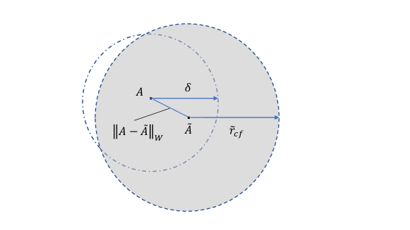
Figure 1: Neighbourhoods of $A$ and $\widetilde{A}$ for which $A(t)$ expected to admit the canonical factorisation. If $\widetilde{A}$ admits a explicit canonical factorisation, then two inequalities: $\|A-\widetilde{A}\|_{W}<\delta$ and $\delta<\tilde{r}_{cf}$ together guarantee that $A$ also possesses the same property. The goal of this paper is to deliver a tool to effectively verify the conditions.

We note that factorisation of an arbitrary strictly nonsingular matrix function $A(t)$ from (1) can be explicitly reduced to factorisation an auxiliary (invertible) matrix function in the form (see section 2 for details):

$$a(t)=\begin{pmatrix}1&\beta_{-}(t)\\ \alpha_{+}(t)&t^{\theta}+\alpha_{+}(t)\beta_{-}(t)\end{pmatrix},$$ (4)

where $\theta={\rm ind}\det a(t)={\rm ind}\det A(t)-2\,{\rm ind}\,a_{11}(t)$.

The approach, highlighted above for matrix function $A(t)$ in its general form, can be applied to the matrix function $a(t)$. As a class $\cal EF$, we take Laurent matrix polynomials in the form:

$$a_{N}(t)=\begin{pmatrix}1&\beta_{-}^{(N)}(t)\\ \alpha_{+}^{(N)}(t)&t^{\theta}+\alpha_{+}^{(N)}(t)\beta_{-}^{(N)}(t)\end{pmatrix},$$ (5)

where $\alpha_{+}^{(N)}(t)$, $\beta_{-}^{(N)}(t)$ are the Laurent polynomials of degree $N$ of the functions $\alpha_{+}(t)$, $\beta_{-}(t)$.

To obtain the explicit estimate of $\|a-a_{N}\|_{W}$, we assume that $a(t)$ is analytical in some annulus containing the unit circle $|t|=1$. In this case, the matrix Fourier coefficients of $a(t)$ coincide with the Laurent coefficients of $a(t)$ and we can use the Cauchy inequalities [24] for the latter.

The factorisation of $a_{N}(t)$ can be explicitly constructed by the method of essential polynomials (see [20, 22, 25]). Moreover, if the Laurent coefficients of $\alpha_{+}^{(N)}(t)$, $\beta_{-}^{(N)}(t)$ belong to the field $\mathbb{Q}(i)$, then the factorisation problem for $a_{N}(t)$ can be solved exactly [19] with help of the package ExactMPF. If the coefficients do not belong the field $\mathbb{Q}(i)$, we can find their rational approximations and to apply ExactMPF. The use of the error-free calculations performed with the package is the key idea of the approach as it guarantees exact computation of the partial indices.

The paper is organised as follows. In the Section 2, we present important facts about the matrix Wiener algebra and the Teoplitz operators used in the following, discuss possible normalisation of the factorisation $A(t)$ and finally show the reduction of an arbitrary strictly nonsingular matrix function (1) to (4). In the section 3, we give the approximation of the matrix function $a(t)$ and estimate its accuracy. Section 4 contains the main result of this article, namely a criterion of the stable factorisation for $a(t)$. In the section 5, we obtain the explicit estimates for the absolute error in the approximate calculation of the factorisation factors. Finally, in the section 6, we present some numerical results highlighting three different cases: canonical factorisation, a factorisation with the equal partial indices and a stable factorisation. Supplementary material collects full set of the data in form of tables.

2 Preliminary considerations

2.1 Main definitions and known facts

In this section, we provide some important definitions and follow the notation from [11, 12, 13, 26].

Let $W^{p\times p}$ be the ${p\times p}$ matrix Wiener algebra consisting of matrix functions with entries from $W$. Thus any $A(t)\in W^{p\times p}$ expands into an absolutely convergent matrix Fourier series, $A(t)=\sum_{k=-\infty}^{\infty}A_{k}t^{k}$, such that $\sum_{k=-\infty}^{\infty}\|A_{k}\|<\infty$. Here, $A_{k}$ belong to the algebra ${\mathbb{C}}^{p\times p}$ complex matrices equipped with the norm represented by any matrix multiplicative norm on ${\mathbb{C}}^{p\times p}$, preserving unity. Algebra $W^{p\times p}$ becomes a Banach algebra if we endow it with a norm $\|A\|_{W}=\sum_{k=-\infty}^{\infty}\|A_{k}\|_{1}$, where $\|\cdot\|_{1}$ is the maximum column sum matrix norm. Also we denote a group of invertible elements of the algebra $W^{p\times p}$ by $GW^{p\times p}$.

If $A_{k}=(a_{ij}^{(k)})_{i,j=1,...,p}$, where $a_{ij}^{(k)}$ are the Fourier coefficients of the element $a_{ij}(t)$ of the matrix function $A(t)$, then it is easily seen that $\|A_{k}\|_{1}\leq\sum_{i,j}|a_{ij}^{(k)}|$. Then $\|A\|_{W}\leq\sum_{i,j}\|a_{ij}\|_{W}$. Let us define

$$W_{+}^{p\times p}=\biggl{\{}A(t)\in W^{p\times p}:A(t)=\sum_{k=0}^{\infty}A_{k}t^{k}\biggr{\}},\\ W_{-}^{p\times p}=\biggl{\{}A(t)\in W^{p\times p}:A(t)=\sum_{k=-\infty}^{0}A_{k}t^{k}\biggr{\}},\\ (W_{-}^{p\times p})_{0}=\biggl{\{}A(t)\in W^{p\times p}:A(t)=\sum_{k=-\infty}^{-1}A_{k}t^{k}\biggr{\}}.$$

It is known that $W_{\pm}^{p\times p}$, $(W_{-}^{p\times p})_{0}$ are closed subalgebras of $W^{p\times p}$ and

$$W^{p\times p}=W_{+}^{p\times p}\ \oplus\ (W_{-}^{p\times p})_{0}.$$

Thus $W_{\pm}^{p\times p}$ is a decomposing algebra.

By ${\cal P}_{+}$ we denote a projector from $W^{p\times p}$ onto $W_{+}^{p\times p}$ along $(W_{-}^{p\times p})_{0}$ and ${\cal P}_{-}={\cal I}-{\cal P}_{+}$. Here ${\cal I}$ is the identity operator. Operator ${\cal P}_{+}$ acts according to the rule

$${\mathcal{P}}_{+}\sum\limits_{k=-\infty}^{\infty}{A_{k}{t}^{k}}=\sum\limits_{k=0}^{\infty}{A_{k}{t}^{k}}.$$

and is a linear bounded operator in $W^{p\times p}$, while $\|\mathcal{P}_{+}\|=1$.

Let $A(t)\in W^{p\times p}$. On the Banach space $W_{+}^{p\times p}$ we define the operator $T_{A}$ acting according to the rule

$$T_{A}X(t)=\mathcal{P}_{+}A(t)X(t).$$

It is obvious that $T_{A}$ is a linear bounded operator and $\|T_{A}\|\leq\|A\|_{W}$. $T_{A}$ is called the Toeplitz operator with the matrix symbol $A(t)$. Note that even though the Toeplitz operator is usually considered on the Banach space $W_{+}^{p\times 1}$, for us it is more convenient to operate on $W_{+}^{p\times p}$. It is straightforward to prove the partial multiplicativity property of the mapping $A\rightarrow T_{A}$, that is, for any $A_{\pm}\in{W_{\pm}}^{p\times p}$ and $B\in W^{p\times p}$, the relations

$$T_{BA_{+}}=T_{B}T_{A_{+}},\ \ T_{A_{-}B}=T_{A_{-}}T_{B}$$

are valid. As a result, all properties of the standard Toeplitz operator are preserved.

We will also need the following two statements.

If $A(t)=A_{-}(t)D(t)A_{+}(t)$ is the right Wiener–Hopf factorisation of an invertible matrix function $A(t)$, then the Toeplitz operator $T_{A}$ is the right (left) invertible if and only if all right partial indices are non-positive (non-negative). In this case $T_{A}^{(-1)}=T_{A_{+}^{-1}}T_{D^{-1}}T_{A_{-}^{-1}}$ is its one-sided inverse [13, ch.VIII, Cor. 4.1]

If a linear bounded operator ${\cal A}$ is one-side invertible, and ${\cal A}^{(-1)}$ is its one-side inverse, then any operator $\widetilde{\cal A}$ satisfying the inequality

$$\|{\cal A}-\widetilde{\cal A}\|<\frac{1}{\|{\cal A}^{(-1)}\|}$$ (6)

is also one-side invertible (from the same side as ${\cal A}$). Moreover, if ${\cal A}$ is one-side invertible but not invertible, then $\widetilde{\cal A}$ is also not invertible [27, ch.II, Th. 5.4]. Note that (6) is true in any elements of an abstract Banach algebra.

2.2 Normalised factorisation of matrix functions

Normalisation of the factorisation plays a crucial role when performing factorisation numerically. This is specifically in case when there is a need to compare the consequent approximations. Usually, a normalisation is chosen ad hock in a line with chosen numerical/asymptotic procedure without any justification and a success depends on each specific case (see for example [28, 29, 30]).

Unfortunately, being important, this issue still has not been fully resolved. The effective results are known for: a) $2\times 2$ matrix functions [31]; for matrix functions of arbitrary dimension $p\times p$ ($p>2$), when b) the set of partial indices are stable [32] or c) all partial indexes are different [33].

Since the paper deals with $2\times 2$ matrices, we present here the normalisation only for such case. Two cases should be distinguished.

• If matrix function admits a factorisation $A(t)=t^{\varkappa_{1}}A_{-}(t)A_{+}(t)$, ($\varkappa_{1}=\varkappa_{2}$) then it can be trivially normalised by the condition $A_{-}(\infty)=I_{2}$, where $I_{2}$ is the unit matrix, and such factorisation is unique.

• In general case ($\varkappa_{1}<\varkappa_{2}$), there exists the so-called $P$-normalised factorisation of $A(t)$ that guarantees its uniqueness [31]. The type of normalisation is determined by a $2\times 2$ permutation matrix $P$, $P=I_{2}$ or $P=J_{2}:=\begin{pmatrix}0&1\\ 1&0\end{pmatrix}$.

The latter can be written in an explicit form: if $\bigl{(}A_{-}(\infty)\bigr{)}_{11}\neq 0$ (or $\bigl{(}A_{-}(\infty)\bigr{)}_{21}\neq 0$), then $A(t)$ admits the $I_{2}$-normalised (or $J_{2}$-normalised) factorisation [31, Th. 2.1].

In a particular case of the stable factorisation ($\rho_{2}-\rho_{1}=1$) when $\bigl{(}A_{-}(\infty)\bigr{)}_{11}$ $\neq 0$, the $I_{2}$-normalisation is carried out as follows (see more details in [31, 32]). Let $A_{-}(t)=A_{0}+A_{1}t^{-1}+\ldots$, and $A_{0}=L_{0}U_{0}$ is $LU$-factorisation of the limiting matrix function $A_{0}=A_{-}(\infty)$. Define a matrix polynomial $Q_{-}(t)=Q_{0}+Q_{1}t^{-1}$ such that

$$Q_{0}=U_{0}^{-1},\ \ Q_{1}=-\frac{1}{(A_{0})_{11}}\begin{pmatrix}0&\bigl{(}A_{1}U_{0}^{-1}\bigr{)}_{12}\\ 0&0\end{pmatrix}.$$ (7)

Let $C_{-}(t)=A_{-}(t)Q_{-}(t)$, $C_{+}(t)=D^{-1}(t)Q_{-}^{-1}(t)D(t)A_{+}(t)$. Then $A(t)=C_{-}(t)D(t)C_{+}(t)$ is the sought for $I_{2}$-normalised factorisation of $A(t)$. $J_{2}$-normalised factorisation constructed analogously by the $JLU$-factorisation of $A_{0}$.

Finally, $P$-normalisation is stable under a small perturbation $A(t)$, that is, for arbitrary sufficiently small $\delta>0$, each matrix function $\widetilde{A}(t)$ possessing the same set of the right partial indices $\rho_{1},\rho_{2}$, as $A(t)$ and satisfying the inequality $\|A-\widetilde{A}\|_{W}<\delta$ has the same type of the $P$-normalisation as $A(t)$ [31, Th. 4.1].

2.3 Reduction of matrix function $A(t)$ to the form $a(t)$

In this subsection, we deliver a representation of the matrix function $A(t)$ given in the form (1) allowing to consider a simpler matrix function, $a(t)$, in the form (4). Let

$$a_{11}(t)=a_{11}^{-}(t)t^{\varkappa}a_{11}^{+}(t),\ \ \Delta(t)=\Delta_{-}(t)t^{\theta+2\varkappa}\Delta_{+}(t)$$ (8)

be the Wiener–Hopf factorisations of the functions $a_{11}(t)$ and $\Delta(t)=\det A(t)$, respectively. Not that the indices $\varkappa$ and $\theta+2\varkappa$ in (8) do not coincide, generally speaking, with the pair $\varkappa_{1}$, $\varkappa_{1}+\varkappa_{2}$ (compare (2)). The only relationship between them is: $\varkappa_{1}+\varkappa_{2}=\theta+2\varkappa$.

The matrix function $A(t)$ can be equivalently written in the form:

$$A(t)=t^{\varkappa}\begin{pmatrix}a_{11}^{-}(t)&0\\ 0&\frac{\Delta_{-}(t)}{a_{11}^{-}(t)}\end{pmatrix}\begin{pmatrix}1&\beta(t)\\ \alpha(t)&\frac{a_{22}a_{11}^{-}a_{11}^{+}}{t^{\varkappa}\Delta_{-}\Delta_{+}}\\ \end{pmatrix}\begin{pmatrix}a_{11}^{+}(t)&0\\ 0&\frac{\Delta_{+}(t)}{a_{11}^{+}(t)}\end{pmatrix},$$ (9)

where

$$\alpha(t)=\frac{a_{11}^{-}(t)a_{21}(t)}{\Delta_{-}(t)t^{\varkappa}a_{11}^{+}(t)},\ \ \beta(t)=\frac{a_{11}^{+}(t)a_{12}(t)}{\Delta_{+}(t)t^{\varkappa}a_{11}^{-}(t)}.$$ (10)

Introducing functions $\alpha_{\pm}(t)=\mathcal{P}_{\pm}\alpha(t)$, $\beta_{\pm}(t)=\mathcal{P}_{\pm}\beta(t)$, matrix function $A(t)$ can be further transformed to the form:

$$A(t)=t^{\varkappa}\begin{pmatrix}a_{11}^{-}(t)&0\\ &\\ \frac{\Delta_{-}(t)\alpha_{-}(t)}{a_{11}^{-}(t)}&\frac{\Delta_{-}(t)}{a_{11}^{-}(t)}\end{pmatrix}a(t)\begin{pmatrix}a_{11}^{+}(t)&\frac{\Delta_{+}(t)\beta_{+}(t)}{a_{11}^{+}(t)}\\ &\\ 0&\frac{\Delta_{+}(t)}{a_{11}^{+}(t)}\end{pmatrix},$$ (11)

where

$$a(t)=\begin{pmatrix}1&0\\ -\alpha_{-}(t)&1\end{pmatrix}\begin{pmatrix}1&\beta(t)\\ \alpha(t)&\frac{a_{22}a_{11}^{-}a_{11}^{+}}{t^{\varkappa}\Delta_{-}\Delta_{+}}\\ \end{pmatrix}\begin{pmatrix}1&-\beta_{+}(t)\\ 0&1\end{pmatrix}.$$ (12)

It remains to observe that this matrix function has the form (4):

$$a(t)=\begin{pmatrix}1&\beta_{-}(t)\\ \alpha_{+}(t)&t^{\theta}+\alpha_{+}(t)\beta_{-}(t)\end{pmatrix}.$$ (13)

For $\theta=0$ this reduction was carried out in [16] where an explicit formulas for the partial indices of $a(t)$ were obtained under additional condition that $\alpha_{+}(t)$ is a polynomial in $t$ or $\beta_{-}(t)$ is a polynomial in $t^{-1}$.

Note that the matrix function $a(t)$ is invertible ($\det a(t)=t^{\theta}$) and thus can be factorised:

$$a(t)=a_{-}(t)d_{r}(t)a_{+}(t),\quad d_{r}(t)={\rm diag}[t^{\rho_{1}},t^{\rho_{2}}],$$ (14)

where $\rho_{1}\leq\rho_{2}$ and $\theta=\rho_{1}+\rho_{2}$.

Comparing the latter with (14) and (11) we conclude that the partial indices of the matrices $A(t)$ and $a(t)$ are related in the following manner:

$$\varkappa_{1}=\varkappa+\rho_{1},\quad\varkappa_{2}=\varkappa+\rho_{2}.$$ (15)

In the following, we will focus on the stable factorisation of the matrix function $a(t)$. Hence,

$$\begin{matrix}\rho_{1}=\rho_{2}=\nu\quad{\rm for\,\,even}\quad\theta=2\nu,\\[5.69054pt] \rho_{1}=\nu,\rho_{2}=\nu+1\quad{\rm for\,\,odd}\quad\theta=2\nu+1.\end{matrix}$$ (16)

As we have already mentioned above, when the authors of [17] built their approximation, they used a completely different representation of the matrix function $A(t)$, in comparison to (11):

$$S(t)=\begin{pmatrix}s_{11}^{+}(t)&0\\ &\\ \frac{t^{-k_{1}}s_{21}(t)}{s_{11}^{-}(t)}&\frac{\Delta^{+}(t)}{s_{11}^{+}(t)}\end{pmatrix}\begin{pmatrix}t^{k_{1}}&0\\ 0&t^{k-k_{1}}\end{pmatrix}\begin{pmatrix}s_{11}^{-}(t)&\frac{t^{-k_{1}}s_{12}(t)}{s_{11}^{+}(t)}\\ &\\ 0&\frac{\Delta^{-}(t)}{s_{11}^{-}(t)}\end{pmatrix},$$

where $s_{11}(t)=s_{11}^{+}(t)t^{k_{1}}s_{11}^{-}$ and $\det{S(t)}=\Delta^{+}(t)t^{k}\Delta^{-}(t)$.

3 Approximation of the matrix function $a(t)$ by the Laurent matrix polynomial $a_{N}(t)$

In this section we approximate $a(t)$ by the Laurent matrix polynomial $a_{N}(t)$ and estimate the norm of the difference $\|a-a_{N}\|_{W}$.

Let $\alpha_{+}(t)=\sum_{k=0}^{\infty}\alpha_{k}t^{k}$ and $\beta_{-}(t)=\sum_{k=-\infty}^{-1}\beta_{k}t^{k}$. We denote

$$\alpha_{+}^{(N)}(t)=\sum_{k=0}^{N}\alpha_{k}t^{k},\ \ \beta_{-}^{(N)}(t)=\sum_{k=-N}^{-1}\beta_{k}t^{k}$$

and consider the Laurent matrix polynomial defined in (5).

Similarly to the matrix function $a(t)$, since $\det a_{N}(t)=t^{\theta}$, then $a_{N}(t)$ is an invertible element of $W^{2\times 2}$ for any $N$.

Now we can estimate the norm $\|a-a_{N}\|_{W}$ as

$$\|a-a_{N}\|_{W}\leq\|\alpha_{+}-\alpha_{+}^{(N)}\|_{W}+\|\beta_{-}-\beta_{-}^{(N)}\|_{W}+\|\alpha_{+}\beta_{-}-\alpha_{+}^{(N)}\beta_{-}^{(N)}\|_{W}.$$

Representing

$$\alpha_{+}(t)\beta_{-}(t)-\alpha_{+}^{(N)}(t)\beta_{-}^{(N)}=\alpha_{+}(t)\Bigl{(}\beta_{-}(t)-\beta_{-}^{(N)}(t)\Bigr{)}+\beta_{-}^{(N)}(t)\Bigl{(}\alpha_{+}(t)-\alpha_{+}^{(N)}(t)\Bigr{)}$$

and taking into account that $\|\beta_{-}^{(N)}\|_{W}\leq\|\beta_{-}\|_{W}$, we get

$$\|a-a_{N}\|_{W}\leq\\ \Bigl{(}1+\|\alpha_{+}\|_{W}\Bigr{)}\|\beta_{-}-\beta_{-}^{(N)}\|_{W}+\Bigl{(}1+\|\beta_{-}\|_{W}\Bigr{)}\|\alpha_{+}-\alpha_{+}^{(N)}\|_{W}.$$ (17)

The last inequality gives us a qualified estimate of the norm of the difference between the matrix functions $a_{N}(t)$ and $a(t)$ defined in (4) and (5), respectively.

To evaluate explicitly the convergence rate, we make additional assumptions on the rate of decay of the Fourier coefficients. Namely, we restrict ourselves to the case when the matrix function $a(t)$ is analytic in the annulus $r_{1}<|t|<r_{2}$ containing the unit circle, $\mathbb{T}$, while $r_{1}$ and $r_{2}$ can be zero and infinity, respectively. This effectively means that the function $\alpha_{+}(t)$ is analytic in the domain $|t|<r_{2}$ while $\beta_{-}(t)$ is analytic in the domain $|t|>r_{1}$.

Obviously, the restriction of $a(t)$ on the unit circle $|t|=1$ belongs to the Wiener algebra $W^{2\times 2}$ and its matrix Fourier coefficients $a_{k}$ coincides with the coefficients of the Laurent series for $a(t)$ in the annulus $r_{1}<|t|<r_{2}$.

The Laurent coefficients $|\alpha_{k}|$ of the function $\alpha_{+}(t)$ hold Cauchy’s inequalities [24]:

$$|\alpha_{k}|\leq\frac{M_{+}(\zeta)}{\zeta^{k}}$$ (18)

for any $\zeta$, $0<\zeta<r_{2}$. Here $M_{+}(\zeta)=\max_{|t|=\zeta}|\alpha_{+}(t)|$.

Fixing a value $\zeta=\zeta_{2}$, $(1<\zeta_{2}<r_{2})$, we can estimate the sums of series $\sum_{k=0}^{\infty}|\alpha_{k}|$, $\sum_{k=N+1}^{\infty}|\alpha_{k}|$ and obtain the following inequalities:

$$\|\alpha_{+}\|_{W}\leq\frac{\zeta_{2}M_{+}(\zeta_{2})}{\zeta_{2}-1},\ \ \|\alpha_{+}-\alpha_{+}^{(N)}\|_{W}\leq\frac{M_{+}(\zeta_{2})}{\zeta_{2}^{N}(\zeta_{2}-1)},M_{+}(\zeta_{2})=\max_{|t|\leq\zeta_{2}}|\alpha_{+}(t)|.$$ (19)

If $r_{2}<\infty$, and $\alpha_{+}(t)$ is continuously extended on $|t|=r_{2}$, then the Cauchy inequalities hold for $\zeta=r_{2}$ and, in this case, we can take also $\zeta_{2}=r_{2}$.

For the function $\beta_{-}(t)$, we can obtain similar estimates fixing a value $\zeta=\zeta_{1}$, ($r_{1}<\zeta_{1}<1$):

$$\|\beta_{-}\|_{W}\leq\frac{\zeta_{1}M_{-}(\zeta_{1})}{1-\zeta_{1}},\ \ \|\beta_{-}-\beta_{-}^{(N)}\|_{W}\leq\frac{\zeta_{1}^{N+1}M_{-}(\zeta_{1})}{(1-\zeta_{1})},$$ (20)

where $M_{-}(\zeta_{1})=\max_{|t|=\zeta_{1}}|\beta_{-}(t)|=\max_{|t|\geq\zeta_{1}}|\beta_{-}(t)|$. If $r_{1}>0$ and $\beta_{-}(t)$ admits a continuous extension on the circle $|t|=r_{1}$, the value $\zeta_{1}=r_{1}$ is also admissible.

This allows us to obtain an explicit estimate (17)

$$\|a-a_{N}\|_{W}\leq\delta_{N}(\zeta_{1},\zeta_{2}),$$ (21)

where $r_{1}<\zeta_{1}<1$, $1<\zeta_{2}<r_{2}$ and

$$\delta_{N}(\zeta_{1},\zeta_{2})=\Bigl{(}1+\frac{\zeta_{2}M_{+}(\zeta_{2})}{\zeta_{2}-1}\Bigr{)}\frac{\zeta_{1}^{N+1}M_{-}(\zeta_{1})}{1-\zeta_{1}}+\Bigl{(}1+\frac{\zeta_{1}M_{-}(\zeta_{1})}{1-\zeta_{1}}\Bigr{)}\frac{M_{+}(\zeta_{2})}{\zeta_{2}^{N}(\zeta_{2}-1)}.$$ (22)

The values $\zeta_{1}=r_{1}$ and $\zeta_{2}=r_{2}$ can be also admissible.

It is obvious that $\delta_{N}(\zeta_{1},\zeta_{2})$ is monotonic decreasing as $N\to\infty$ and tends to zero for any fixed $\zeta_{1},\zeta_{2}$. Although, if $\zeta_{1}$, $\zeta_{2}$ are close enough to $1$, then the convergence is slow. On the other hand, the function increase when $\zeta_{1}$ or $\zeta_{2}$ are close to the other ends of their intervals. Therefore, it is desirable to optimize the choice $\zeta_{1}$, $\zeta_{2}$ minimizing the function $\delta_{N}(\zeta_{1},\zeta_{2})$ on the rectangle $(r_{1},1)\times(1,r_{2})$. Depending on whether the series converge on the closed or open domain, we can distinguish four respective cases.

1. $r_{1}>0,r_{2}<\infty$, that is, the function $\alpha_{+}(t)$ is analytic into $|t|<r_{2}$, and $\beta_{-}(t)$ is analytic into $|t|>r_{1}$.

2. $r_{1}>0,r_{2}=\infty$, that is, the function $\alpha_{+}(t)$ is an entire function, and $\beta_{-}(t)$ is analytic into $|t|>r_{1}$.

3. $r_{1}=0,r_{2}<\infty$, that is, the function $\alpha_{+}(t)$ is analytic into $|t|<r_{2}$, and $\beta_{-}(t)$ is analytic into $\overline{\mathbb{C}}\setminus\{0\}$.

4. $r_{1}=0,r_{2}=\infty$, that is, the function $\alpha_{+}(t)$ is an entire function, and $\beta_{-}(t)$ is analytic into $\overline{\mathbb{C}}\setminus\{0\}$.

In order to effectively use (22), we need to estimate $M_{-}(\zeta_{1})$, $M_{+}(\zeta_{2})$ in the respective domains with the best possible accuracy. Here a difficulty steams from the fact that the minimization is sought in the open set $(r_{1},1)\times(1,r_{2})$. In practice we restrict ourselves to a closed rectangular $K$ embedded into $(r_{1},1)\times(1,r_{2})$ that provides quite a reasonable approximation.

4 A criterion of the stable factorisation for the matrix function $a(t)$

Having constructed a Laurent matrix polynomial (5) of degree $N$, that is an approximant of the matrix function (4) allowing for a stable factorisation

as is described in the section 3 above, we can compute the following measure:

$$q_{N}(\zeta_{1},\zeta_{2})=\sigma\,\delta_{N}(\zeta_{1},\zeta_{2})\|\bigl{(}a_{+}^{(N)}\bigr{)}^{-1}\|_{W}\,\|\bigl{(}a_{-}^{(N)}\bigr{)}^{-1}\|_{W},$$ (23)

where

$$\sigma=\|d_{r}\|_{W}=\|d_{r}^{-1}\|_{W}=\begin{cases}1,&\text{if $\theta=2\nu$},\\ 2,&\text{if $\theta=2\nu+1$.}\end{cases}$$ (24)

Theorem 4.1.

Let $a(t)$ admits a stable factorisation (14) and the factorisation is $P$-normalised. Then, there exists a natural $N_{0}$ such that, for $N>N_{0}$ and for all admissible pairs $(\zeta_{1},\zeta_{2})$, the following conditions are fulfilled

1. $a_{N}(t)$ admits a stable $P$-normalised factorisation:

   $$a_{N}(t)=a_{-}^{(N)}(t)d_{r}(t)a_{+}^{(N)}(t),$$ (25)

2. $q_{N}(\zeta_{1},\zeta_{2})<1$.

Proof.

Since the sequence $a_{N}(t)$ converges to the matrix function $a(t)$ admitting a stable factorisation, it is always possible to find a natural $N_{0}$ such that, for all $N>N_{0}$, $a_{N}(t)$ admits the same factorisation (the same set of partial indices) [1]. However, to deliver an estimate for the stability domain, more accurate analysis is required. This is the aim of this theorem.

Since $a_{N}(t)$ converges to the matrix function $a(t)$ there exists an integer $N_{0}$ such that

$$\|a(t)-a_{N}\|_{W}<\frac{1}{\sigma\|a_{+}^{-1}\|_{W}\|a_{-}^{-1}\|_{W}},\ \ \text{if}\ \ N\geq N_{0}.$$ (26)

From (26) and (24), it follows that

$$\|a-a_{N}\|_{W}<\frac{1}{\|a^{-1}\|_{W}},\ \ \text{if}\ \ N\geq N_{0}.$$

The latter means that $a_{N}(t)$ is an invertible element of $W^{2\times 2}$ and thus, it admits a factorisation $a_{N}(t)=a_{-}^{(N)}(t)d_{r}^{(N)}(t)a_{+}^{(N)}(t)$. The next step in the proof is to demonstrate that the latter inequality guarantees also that $a_{N}(t)$ belongs to the stability region (or equivalently, $d_{r}^{(N)}(t)=d_{r}(t))$.

By the assumption of the theorem, the matrix function $a(t)$ admits the stable factorisation $a(t)=a_{-}(t)d_{r}(t)a_{+}(t)$, that is $d_{r}(t)=t^{\nu}I_{2}$ if $\theta=2\nu$, and $d_{r}(t)=t^{\nu}\begin{pmatrix}1&0\\ 0&t\end{pmatrix}$ for $\theta=2\nu+1$. Moreover, since we consider the right partial indices of the matrix function $a(t)$, they are both non-negative for $\nu\geq 0$ and non-positive for $\nu<0$. We will demonstrate now that $d_{r}^{(N)}(t)=d_{r}(t)$.

Let us consider Toeplitz operators $T_{a}$ and $T_{a_{N}}$ with the symbols $a(t)$ and $a_{N}(t)$, respectively. Since the partial indices have the same sign, then the operator $T_{a}$ is one-sided invertible (invertible if $\nu=0$ ) and $T^{(-1)}_{a}=T_{a_{+}^{-1}}T_{d_{r}^{-1}}T_{a_{-}^{-1}}$ is its one-sided inverse (inverse in the case $\nu=0$), moreover (see [13])

$$\|T^{(-1)}_{a}\|\leq\|T_{a_{+}^{-1}}\|\|T_{d_{r}^{-1}}\|\|T_{a_{-}^{-1}}\|\leq\sigma{\|a_{+}^{-1}\|_{W}\|a_{-}^{-1}\|_{W}}.$$

Then, from (26), we have

$$\|T_{a}-T_{a_{N}}\|\leq\|a-a_{N}\|_{W}<\frac{1}{\sigma\|a_{+}^{-1}\|_{W}\|a_{-}^{-1}\|_{W}}\leq\frac{1}{\|T^{(-1)}_{a}\|}.$$

This in turn means that the operator $T_{a_{N}}$ is also one-side invertible (or invertible if $\nu=0$). Moreover, the operators $T_{a}$ and $T_{a_{N}}$ are invertible from the same side and, therefore, in the factorisation $a_{{N}}(t)=a_{-}^{(N)}(t)d_{r}^{(N)}(t)a_{+}^{(N)}(t)$, $d_{r}^{(N)}(t)={\rm diag}[t^{{\widetilde{\rho}_{1}}},t^{{\widetilde{\rho}_{2}}}]$, indices $\widetilde{\rho}_{1},\widetilde{\rho}_{2}$ have the same signs as $\rho_{1},\rho_{2}$.

The following three cases are possible:
1) If $a(t)$ admits the canonical factorisation, i.e. $\nu=0$, then $T_{a_{N}}$ is invertible and, hence, $a_{N}(t)$ admits also the canonical factorisation.
2) Let $a(t)$ admits a stable factorisation and $\theta=2\nu$, that is $d_{r}(t)=t^{\nu}I_{2}$. Consider auxiliary matrix functions $b(t)=t^{-\nu}a(t)$ and $c(t)=t^{-\nu}a_{N}(t)$. By the construction, $b(t)$ admits a canonical factorisation, $b(t)=a_{-}(t)a_{+}(t)$. On the other hand, since $\|t^{\nu}\|_{W}=\|t^{-\nu}\|_{W}=1$ and, due to inequality (26), we conclude

$$\|b-c\|_{W}<\frac{1}{\|b_{+}^{-1}\|_{W}\|b_{-}^{-1}\|_{W}}.$$

Hence, (see the previous case), $c(t)$ also admits a canonical factorisation, $a_{N}(t)=t^{\nu}c(t)$ and $d_{r}^{(N)}(t)=d_{r}(t)$.
3) Finally, let $a(t)$ admits a stable factorisation and $\theta=2\nu+1$, i.e. $d_{r}(t)=t^{\nu}\begin{pmatrix}1&0\\ 0&t\end{pmatrix}$. Consider again the matrix functions $b(t)=t^{-\nu}a(t)$ and $c(t)=t^{-\nu}a_{N}(t)$. The auxiliary matrix function $b(t)=a_{-}(t)\begin{pmatrix}1&0\\ 0&t\end{pmatrix}a_{+}(t)$ admits a stable factorisation, and

$$\|b-c\|_{W}<\frac{1}{2\|b_{+}^{-1}\|_{W}\|b_{-}^{-1}\|_{W}}.$$

This proves that the respective operators are invertible from the same side, and their right indices are non negative. Thus, we conclude that $\widetilde{\rho}_{1}\geq\nu$ and $\widetilde{\rho}_{2}>\nu$, and, since $\widetilde{\rho}_{1}+\widetilde{\rho}_{2}=2\nu+1$, this is possible only if $\widetilde{\rho}_{1}=\nu,\widetilde{\rho}_{2}=\nu+1$. This finishes the proof.

Summarising, we have shown that, under condition (26) the approximate matrix function $a_{N}(t)$ admits a stable factorisation with the same set of stable partial indices as the original matrix function $a(t)$.

It remains to prove the second statement of the Theorem. Let $N\geq N_{0}$ and $a_{N}(t)=a_{-}^{(N)}(t)d_{r}(t)a_{+}^{(N)}(t)$ is now the stable $P$-normalised factorisation of $a_{N}(t)$. It follows from Th. 5.1 of [31] that the factors $a_{\pm}^{(N)}(t)$ converge to normalised $a_{\pm}(t)$ as $N\to\infty$. Hence, the sequence $\|\bigl{(}a_{+}^{(N)}\bigr{)}^{-1}\|_{W}\cdot\|\bigl{(}a_{-}^{(N)}\bigr{)}^{-1}\|_{W}$ is bounded. As we noted in the previous section, the sequence $\delta_{N}(\zeta_{1},\zeta_{2})$ monotonically tends to zero for any fixed pair $(\zeta_{1},\zeta_{2})$. Hence, starting from some $N$ the inequality $q_{N}(\zeta_{1},\zeta_{2})<1$ is fulfilled. ∎

Theorem 4.2.

If conditions 1)–2) are fulfilled for at least one $N$ and one admissible pair $(\zeta_{1},\zeta_{2})$, then $a(t)$ admits the stable factorisation with the same set of partial indices as $a_{N}(t)$.

Proof.

Since $\det a_{N}(t)=t^{\theta}$, $a_{N}(t)$ is invertible in the algebra $W^{2\times 2}$ for any $N$. Suppose that there exists $N$ such that $a_{N}(t)$ admits a stable $P$-normalised factorisation $a_{N}(t)=a_{-}^{(N)}(t)d_{r}(t)a_{+}^{(N)}(t),$ and for some $(\zeta_{1},\zeta_{2})$ it is fulfilled the inequality

$$\delta_{N}(\zeta_{1},\zeta_{2})<\frac{1}{\sigma\|\bigl{(}a_{+}^{(N)}\bigr{)}^{-1}\|_{W}\|\bigl{(}a_{-}^{(N)}\bigr{)}^{-1}\|_{W}},$$ (27)

that coincides with $q_{N}<1$ (compare (23))

$$\|a-a_{N}\|_{W}\leq\delta_{N}(\zeta_{1},\zeta_{2})<\frac{1}{\sigma\|\bigl{(}a_{+}^{(N)}\bigr{)}^{-1}\|_{W}\,\|\bigl{(}a_{-}^{(N)}\bigr{)}^{-1}\|_{W}}.$$ (28)

Now we carry out the same reasoning as in the proof of the Theorem 4.1, only interchanging $a(t)$ by $a_{N}(t)$. Thus, in virtue of (28) we have

$$\|T_{a}-T_{a_{N}}\|\leq\|a-a_{N}\|_{W}<\frac{1}{\|\bigl{(}a_{+}^{(N)}\bigr{)}^{-1}\|_{W}\|d_{r}(t)\|_{W}\|\bigl{(}a_{-}^{(N)}\bigr{)}^{-1}\|_{W}}.$$ (29)

Since $a_{N}(t)$ admits the stable factorisation, the operator $T_{a_{N}}$ is one-side invertible, and $T_{a_{N}}^{(-1)}=T_{(a_{+}^{(N)})^{-1}}T_{d_{r}^{-1}}T_{(a_{-}^{(N)})^{-1}}$ is its one-side inverse.

Now from (29) it follows that $\|T_{a}-T_{a_{N}}\|<\frac{1}{\|T_{a_{N}}^{(-1)}\|}.$ This, in turn, means that the operator $T_{a}$ is one-side invertible. The same arguments as above show that the matrix function $a(t)$ admits the stable factorisation. ∎

Remark 4.1.

The normalisation of the factorisation is used only in the proof of necessity of conditions 1)-2). In fact, in the Theorem 4.1 we can omit the $P$-normalisation requirement and require that the sequence $\|\bigl{(}a_{+}^{(N)}\bigr{)}^{-1}\|_{W}$ $\|\bigl{(}a_{-}^{(N)}\bigr{)}^{-1}\|_{W}$ is bounded from above. In the Theorem 4.2 we can use any factorisation. This allows us to avoid the computational difficulties associated with the procedure of $P$-normalisation. However, $P$-normalisation is a mandatory step in constructing an approximate factorisation with the guaranteed accuracy.

Remark 4.2.

Those theorems allow us to formulate a criterion for the case when matrix function $a(t)$ does not admit a stable factorisation. However, this would require checking an infinite number of conditions (for each $N$) and, thus, is unlikely to be implemented in practice.

In fact, the results provided in the Sections 3 and 4 allow to address the main challenge of this paper, providing two explicit conditions $\|a-a_{N}\|_{W}<\delta_{N}(\zeta_{1},\zeta_{2})$ and $q_{N}<1$ that a) can be numerically verified and b) guarantee that matrix function $a(t)$ has the same set of stable partial indices as $a_{N}(t)$. To highlight things even further, we note that they represent those inequalities, $\|a-a_{N}\|_{W}<\delta$ and $\delta<\tilde{r}_{cf}$, discussed around the Figure 1. Indeed, the inequality $q_{N}<1$ can be equivalently written in the form (27) where the right-hand side corresponds to the stability radius $\tilde{r}_{sf}$. The conditions are sufficient for stability the numerical procedure used in the approximate factorisation while continuity of the factors has been proven in [31, Th. 5.1]. However, the quality of the approximation remains unknown and thus, if the procedure does not converge fast enough, this might be a serious obstacle for computations.

Having a solid theoretical estimate for the convergence rate is always a benefit. Next section is devoted to this task for a classic canonical case ($\varkappa_{1}=\varkappa_{2}=0$) and a generalised canonical one ($\varkappa_{1}=\varkappa_{2}$). Unfortunately, the remaining stable case ($\theta=2\nu+1$) requires more delicate treatment.

5 Accuracy estimate of the factors in approximation of a canonical factorisation

In the first subsection, we briefly recall results of the work [34] on the continuity of factors $A_{\pm}(t)$ of the classic canonical factorisation (all partial indices are zero) and improve explicit estimates for the norm $\|A_{\pm}-A_{\pm}^{(N)}\|_{W}$ presented therein. Bearing in mind possible applications, we provide the analysis for matrix functions of an arbitrary order $p\geq 2$.

5.1 Explicit estimates for the factors of canonical factorisation of the original matrix function $A(t)$.

We will assume that the canonical factorisation $A(t)=A_{-}(t)A_{+}(t)$ is normalised by the condition $A_{-}(\infty)=A_{0}$, where $A_{0}$ is an arbitrary, predetermined, invertible matrix. This normalisation guarantees the uniqueness of the canonical factorisation. Clearly, we can choose a unit matrix as the limiting value for the factor ($A_{0}=I_{p}$), however, since the proof is not much dependent in this case of the normalisation we stay with more general formulation.

We need the following elementary lemmas. Their proofs for $q=1/2$ are given in [34]. Even the proofs do not differ much in the general case, the new results represent an improvement allowing to deliver the estimates in more convenient for practical use.

Lemma 5.1.

Let $\mathcal{A}$ be an invertible bounded linear operator in some Banach space and and the operator $\widetilde{\mathcal{A}}$ satisfies the inequality

$$\|\mathcal{A}-\widetilde{\mathcal{A}}\|\leq\frac{q}{\|{\mathcal{A}}^{-1}\|},\quad 0<q<1.$$ (30)

Then $\widetilde{\mathcal{A}}$ is also invertible and, for solutions of the equations $\mathcal{A}x=b$, $\widetilde{\mathcal{A}}\widetilde{x}=\widetilde{b}$ the following estimate holds true

$$\|x-\widetilde{x}\|\leq\frac{\|{\mathcal{A}}^{-1}\|}{1-q}\left(\|b\|\,\|{\mathcal{A}}^{-1}\|\,\|\mathcal{A}-\widetilde{\mathcal{A}}\|+\|b-\widetilde{b}\|\right).$$

Lemma 5.2.

Let the element $\mathcal{A}$ of a Banach algebra is invertible and the element $\widetilde{\mathcal{A}}$ satisfies the inequality (30). Then $\widetilde{\mathcal{A}}$ is invertible element and

$$\|{\mathcal{A}}^{-1}-\widetilde{\mathcal{A}}^{-1}\|\leq\frac{1}{1-q}\,\|\mathcal{A}^{-1}\|^{2}\cdot\|{\mathcal{A}}-\widetilde{\mathcal{A}}\|.$$

Theorem 5.1.

Let $A(t)\in GW^{p\times p}$ admits the canonical factorisation $A(t)=A_{-}(t)A_{+}(t)$ and this factorisation is normalised by the condition $A_{-}(\infty)=A_{0}$. If the matrix function $\widetilde{A}(t)\in W^{p\times p}$ satisfies the inequality

$${\|A-\widetilde{A}\|}_{W}\leq\frac{q}{{\|A_{+}^{-1}\|}_{W}{\|A_{-}^{-1}\|}_{W}},\quad 0<q<1,$$ (31)

then $\widetilde{A}(t)$ is an invertible matrix function that admits the canonical factorisation $\widetilde{A}(t)=\widetilde{A}_{-}(t)\widetilde{A}_{+}(t).$ For the unique factorisation normalised by the same condition $\widetilde{A}_{-}(\infty)=A_{0}$, the following estimates are valid:

$$(i)\quad{\|A_{+}^{-1}-\widetilde{A}_{+}^{-1}\|}_{W}\leq\frac{\|A_{0}\|}{1-q}\,{\|A_{+}^{-1}\|}_{W}^{2}\,{\|A_{-}^{-1}\|}_{W}^{2}{\|A-\widetilde{A}\|}_{W},$$ (32)

$$(ii)\quad{\|A_{-}-\widetilde{A}_{-}\|}_{W}\leq\biggl{(}\|A_{+}^{-1}\|_{W}+\frac{\|A_{0}\|\|A\|_{W}}{1-q}\|A_{+}^{-1}\|_{W}^{2}{\|A_{-}^{-1}\|}_{W}^{2}+\\ +\frac{q}{1-q}\|A_{0}\|\|A_{+}^{-1}\|_{W}{\|A_{-}^{-1}\|}_{W}\biggr{)}\|A-\widetilde{A}\|{{}_{W},}$$ (33)

Moreover, if condition (31) is replaced by a stronger one:

$${\|A-\widetilde{A}\|}_{W}\leq\frac{q}{\|A_{+}^{-1}\|_{W}{\|A_{-}^{-1}\|}_{W}}\cdot\frac{(1-q)}{{\|A_{0}\|\|A_{-}^{-1}\|_{W}}\|A_{+}\|_{W}\|A^{-1}_{+}\|_{W}},$$ (34)

then

$$(iii)\quad{\|A_{+}-\widetilde{A}_{+}\|}_{W}\leq\frac{\|A_{0}\|}{(1-q)^{2}}{\|A_{+}\|}_{W}^{2}{\|A_{+}^{-1}\|}_{W}^{2}{\|A_{-}^{-1}\|}_{W}^{2}\|{\|A-\widetilde{A}\|}_{W}.$$ (35)

Proof.

To prove the first inequality (32), we consider operator equations $T_{A}X=A_{0}$ and $T_{\widetilde{A}}\widetilde{X}=A_{0}$, that both have unique solutions. These solutions are matrix functions $X=A_{+}^{-1}$ and $\widetilde{X}=\widetilde{A}_{+}^{-1}$, respectively. Indeed, $T_{A}A_{+}^{-1}=T_{A_{-}}T_{A_{+}}A_{+}^{-1}=\mathcal{P}_{+}A_{-}\mathcal{P}_{+}A_{+}A_{+}^{-1}=\mathcal{P}_{+}A_{-}I_{p}=\mathcal{P}_{+}A_{-}=A_{-}(\infty)=A_{0}$. Similar arguments apply for the second equation.

Utilising Lemma 5.1 with $b=\widetilde{b}=A_{0}$, we have

$${\|A_{+}^{-1}-\widetilde{A}_{+}^{-1}\|}_{W}={\|X-\widetilde{X}\|}_{W}\leq\frac{\|A_{0}\|}{1-q}\,{\|T_{A}^{-1}\|}^{2}\,\|T_{A}-T_{\widetilde{A}}\|.$$

Finally, since $\|T_{A}^{-1}\|\leq{\|A_{+}^{-1}\|}_{W}{\|A_{-}^{-1}\|}_{W}$ and $\|T_{A}-T_{\widetilde{A}}\|\leq{\|A-\widetilde{A}\|}_{W}$, we arrive at (32).

Now we can prove the continuity of the factor $A_{-}$ with its explicit estimate (ii). Since both matrix functions $A(t)$ and $\tilde{A}(t)$ admit canonical factorisations, the following identity is valid:

$${{A}_{-}}-{{\widetilde{A}}_{-}}=(A-\widetilde{A})A_{+}^{-1}+\widetilde{A}(A_{+}^{-1}-\widetilde{A}_{+}^{-1}),$$

leading to the inequality

$${\|A_{-}-\widetilde{A}_{-}}\|_{W}\leq{\|A_{+}^{-1}\|}_{W}\|A-\widetilde{A}\|+\|\widetilde{A}\|_{W}\|A_{+}^{-1}-\widetilde{A}_{+}^{-1}\|.$$ (36)

Utilising (31), we get an estimate of the first multiplayer of the second term, $\|\widetilde{A}\|_{W}$, in the equality (36) in the form

$$\|\widetilde{A}\|_{W}\leq\|A\|_{W}+{\|A-\widetilde{A}\|}_{W}\leq\|A\|_{W}+\frac{q}{{\|A_{+}^{-1}\|}_{W}{\|A_{-}^{-1}\|}_{W}},$$

while the statement (i) of this theorem provides an estimate for the second multiplayer. Substituting those two inequalities into (36) we arrive at (33).

Finally, we can prove the statement (iii), that represents an explicit stability condition for the factor $A_{+}(t)$ for a small perturbation of the matrix function $A(t)$.

Since condition (34) is stronger than (31), it also guarantees an existence of the canonical factorisation $\widetilde{A}(t)$ fixed by its limiting value $A_{-}(\infty)=A_{0}$. Utilising Lemma 5.2 to elements $\mathcal{A}=A_{+}^{-1}(t)$, $\widetilde{\mathcal{A}}=\widetilde{A}_{+}^{-1}(t)$ considered in the Banach algebra $W_{+}^{p\times p}$, and taking into account the statement (i), that is the inequality (32) proven above, we arrive at (35). Condition (30) is fulfilled if we take a new radius of the vicinity of $A(t)$. ∎

To finalise this subsection, we note that the explicit estimates for the absolute errors $\|A_{+}-\widetilde{A}_{+}\|_{W},\,\|A_{-}-\widetilde{A}_{-}\|_{W}$ were obtained only for canonical factorisation of the original matrix function $A(t)$ of an arbitrary size $p\times p$.

5.2 An explicit estimates for factors $a_{\pm}(t)$ for matrix function $a(t)$ from (4)

In this subsection, we specify the results for matrix function $a(t)$ in the form (4) for $\theta=2\nu$ and assume that the partial indices are equal. Then we can always consider a new matrix function $b(t)=t^{-\nu}a(t)$ admitting classic canonical factorisation ($\theta=0$). Below, we assume without lost of generality, that $\theta=0$ for both matrix functions $a(t)$ and $a_{N}(t)$. We will assume that the factorisation is normalized by the condition $a_{-}^{(N)}(\infty)=I_{2}$. Applying Th.5.1 to the matrix function $a_{N}(t)$, we can formulate

Corollary 5.1.

Let for some $N$, $\zeta_{1},\zeta_{2}$ we have $\|a-a_{N}\|_{W}<\delta_{N}(\zeta_{1},\zeta_{2}),$ $a_{N}(t)$ admits the canonical factorisation. Then

$$\|a_{+}^{-1}-(a_{+}^{(N)})^{-1}\|_{W}<\frac{\|(a_{+}^{(N)})^{-1}\|_{W}^{2}\,\|(a_{-}^{(N)})^{-1}\|_{W}^{2}}{1-q_{N}(\zeta_{1},\zeta_{2})}\delta_{N}(\zeta_{1},\zeta_{2}),$$ (37)

if $q_{N}(\zeta_{1},\zeta_{2}):=\delta_{N}(\zeta_{1},\zeta_{2})\|\bigl{(}a_{+}^{(N)}\bigr{)}^{-1}\|_{W}\,\|\bigl{(}a_{-}^{(N)}\bigr{)}^{-1}\|_{W}<1$;

$$\|a_{-}-a_{-}^{(N)}\|_{W}<\delta_{-}=\Bigl{(}\|(a_{+}^{(N)})^{-1}\|_{W}+\frac{\|a_{N}\|_{W}\,\|(a_{+}^{(N)})^{-1}\|_{W}^{2}\|(a_{-}^{(N)})^{-1}\|_{W}^{2}}{1-q_{N}(\zeta_{1},\zeta_{2})}+\\ \frac{q_{N}(\zeta_{1},\zeta_{2})\,\|(a_{+}^{(N)})^{-1}\|_{W}\,\|(a_{-}^{(N)})^{-1}\|_{W}}{1-q_{N}(\zeta_{1},\zeta_{2})}\Bigr{)}\delta_{N}(\zeta_{1},\zeta_{2}),$$ (38)

if $q_{N}(\zeta_{1},\zeta_{2})<1$;

$$\|a_{+}-a_{+}^{(N)}\|_{W}<\delta_{+}=\frac{\|a_{+}^{(N)}\|_{W}^{2}\,\|(a_{+}^{(N)})^{-1}\|_{W}^{2}\,\|(a_{-}^{(N)})^{-1}\|_{W}^{2}}{{\bigl{(}1-q^{+}_{N}(\zeta_{1},\zeta_{2})\bigr{)}^{2}}}\delta_{N}(\zeta_{1},\zeta_{2}),$$ (39)

if $\gamma_{N}(\zeta_{1},\zeta_{2}):=4\delta_{N}(\zeta_{1},\zeta_{2}){\|a_{+}^{(N)}\|_{W}\|(a_{+}^{(N)})^{-1}\|_{W}^{2}\|(a_{-}^{(N)})^{-1}\|_{W}^{2}}\leq 1.$

Here $q^{+}_{N}(\zeta_{1},\zeta_{2})=\frac{1}{2}\bigl{(}1-\sqrt{1-\gamma_{N}(\zeta_{1},\zeta_{2})}\,\bigr{)}.$

Proof.

The proof is required only for estimate (39). Let us define the parameter $q^{+}_{N}(\zeta_{1},\zeta_{2})$ by the equation

$$q(1-q){=}\frac{1}{4}\gamma_{N}(\zeta_{1},\zeta_{2}).$$ (40)

Since $\max_{[0,1]}q(1-q)=\frac{1}{4}$, the condition $\gamma_{N}(\zeta_{1},\zeta_{2})\leq 1$ must be met. We have two roots of Eq.(40), but the root is such that $0<q\leq 1/2$, that is $q^{+}_{N}(\zeta_{1},\zeta_{2})=\frac{1}{2}\bigl{(}1-\sqrt{1-\gamma_{N}(\zeta_{1},\zeta_{2})}\,\bigr{)}$, gives the better estimate for $\|a_{+}-a_{+}^{(N)}\|_{W}$. Now all conditions of Th.5.1, item (iii), are fulfilled and applying it we arrive to (39). ∎

Note that, since the factorisation problem for a Laurent matrix polynomial $a_{N}(t)$ can be solved explicitly (see [22]), the estimates for $\|a_{-}-a_{-}^{(N)}\|_{W}$ and $\|a_{+}-a_{+}^{(N)}\|_{W}$ can be obtained constructively in terms of some characteristics of the functions $\alpha_{+}(t)$, $\beta_{-}(t)$.

Suppose that the Laurent coefficients of $\alpha_{+}^{(N)}(t)$, $\beta_{-}^{(N)}(t)$ belong to the field $\mathbb{Q}(i)$. Since $\det a_{N}(t)=1$, the factorisation problem for $a_{N}(t)$ can be solved exactly [19]. We can construct the exact factorisation with help of the package ExactMPF [19]. If the Laurent coefficients $\alpha_{k}$, $\beta_{k}$ do not belong the field $\mathbb{Q}(i)$, we can find the best rational approximations for them and include the respective corrections in $\delta_{N}(\zeta_{1},\zeta_{2})$.

6 Numerical experiments

6.1 Matrix function admitting canonical factorisation ($\theta=0$).

First we consider matrix function $a(t)$:

$$a(t)=\begin{pmatrix}1&t^{-2}\sqrt{k_{1}^{2}-t^{2}}\\[5.69054pt] \sqrt{k_{2}^{2}-t^{2}}&1+t^{-2}\sqrt{k_{2}^{2}-t^{2}}\sqrt{k_{1}^{2}-t^{2}}\end{pmatrix},\quad k_{1}^{-1},k_{2}>1.$$ (41)

Here, $\alpha_{+}(t)$ is the branch of $\sqrt{k_{2}^{2}-t^{2}}$, $k_{2}>1$, that is analytic into the domain $\mathbb{C}\setminus\bigl{(}(-\infty,-k_{2})\cup(k_{2},+\infty)\bigr{)}$, and has the positive value at $t=0$.

For the function $\beta_{-}(t)=t^{-2}\sqrt{k_{1}^{2}-t^{2}}$, $k_{1}<1$, we consider the branch of the square root $\sqrt{k_{1}^{2}-t^{2}}$ with the cut $(-k_{1},k_{1})$ fixed by value of $t^{-1}\sqrt{k_{1}^{2}-t^{2}}$ at $t=\infty$ equal to $i$.

The function $\alpha_{+}(t)$ is expanded into the series

$$\alpha_{+}(t)=k_{2}\Bigl{(}1-\frac{t^{2}}{2k_{2}^{2}}-\sum_{n=2}^{\infty}\frac{(2n-3)!!}{(2n)!!}\frac{t^{2n}}{k_{2}^{2n}}\Bigr{)},$$

that converges absolutely in the closet disk $|t|\leq k_{2}$. So, $\alpha_{+}(t)$ is continuous on $|t|\leq k_{2}$, analytic into $|t|<k_{2}$, and $\alpha_{+}(t)$, $|t|=1$, belongs the subalgebra $W_{+}$. We can easily prove that $M_{+}(\zeta_{2})=\sqrt{k_{2}^{2}+\zeta_{2}^{2}}$ for $1<\zeta_{2}\leq k_{2}$, where function $M_{+}(\zeta_{2})$ has been defined in (18).

Function $\beta_{-}(t)$ is expanded into the series

$$\beta_{-}(t)=\frac{i}{t}\Bigl{(}1-\frac{k_{1}^{2}}{2t^{2}}-\sum_{n=2}^{\infty}\frac{(2n-3)!!}{(2n)!!}\frac{k_{1}^{2n}}{t^{2n}}\Bigr{)},$$

that converges absolutely in the close domain $|t|\geq k_{1}$. Moreover, $\beta_{-}(t)$ is continuous on $|t|\geq k_{1}$, analytic into $|t|>k_{1}$, and $\beta_{-}(t)$, $|t|=1$, belongs the subalgebra $W_{-}^{0}$. It is easy to prove that $M_{-}(\zeta_{1})=\frac{\sqrt{k_{1}^{2}+\zeta_{1}^{2}}}{\zeta_{1}^{2}}$ for $k_{1}\leq\zeta_{1}<1$. Thus, the admissible pairs $(\zeta_{1},\zeta_{2})$ belong to the rectangular $[k_{1},1)\times(1,k_{2}]$.

Now we have $\|a-a_{N}\|_{W}<\delta_{N}(\zeta_{1},\zeta_{2})$ for $k_{1}\leq\zeta_{1}<1$, $1<\zeta_{2}\leq k_{2}$, with the parameter $\delta_{N}(\zeta_{1},\zeta_{2})$ defined in (22)

$$\delta_{N}(\zeta_{1},\zeta_{2})=\\ \Biggl{(}1+\frac{\zeta_{2}\sqrt{k_{2}^{2}+\zeta_{2}^{2}}}{\zeta_{2}-1}\Biggr{)}\frac{\zeta_{1}^{N-1}\sqrt{k_{1}^{2}+\zeta_{1}^{2}}}{1-\zeta_{1}}+\Biggl{(}1+\frac{\sqrt{k_{1}^{2}+\zeta_{1}^{2}}}{\zeta_{1}(1-\zeta_{1})}\Biggr{)}\frac{\sqrt{k_{2}^{2}+\zeta_{2}^{2}}}{\zeta_{2}^{N}(\zeta_{2}-1)}.$$ (42)

Since the optimal choice of the parameters $\zeta_{1},\zeta_{2}$ is desirable but not mandatory, we choose as optimal values $\zeta_{1},\zeta_{2}$ the solution of the minimization problem on a compact set $[k_{1},1-\epsilon]\times[1+\epsilon,k_{2}]$ for sufficiently small $\epsilon>0$. For these purposes we use the package Optimization of the system Maple.

Example 6.1.

Now we present an approximate factorisation of matrix function (41) with a guaranteed accuracy for a fixed values of $k_{1}=1/5$, $k_{2}=5$. With help procedure Minimize of the package Optimization we verify that, for $\epsilon=0.01$ and for all $N\in[1,100]$, optimal values are $\zeta_{1}=1/5$, $\zeta_{2}=5$, thus

$$\delta_{N}(1/5,5)=\frac{15+2\sqrt{2}}{4}\cdot 5^{1-N}\approx 22.2855\cdot 5^{-N}.$$ (43)

For any fixed $N_{0}$ and $1\leq N\leq N_{0}$, the evident inequality

$$\|a_{N_{0}}-a_{N}\|_{W}\leq\|a-a_{N}\|_{W}\leq\delta_{N}.$$ (44)

We found the norms $\|a_{30}-a_{N}\|_{W}$, $\|a_{40}-a_{N}\|_{W}$, $\|a_{50}-a_{N}\|_{W}$ and compared them with the calculated values of $\delta_{N}$ for $N\in[1,30]$. The results are shown in Figure 2 and Table 1. All calculations were carried out with $\rm Digits=10$. The values for $\|a_{50}-a_{N}\|_{W}$ completely coincide with $\|a_{40}-a_{N}\|_{W}$. As a result, we conclude that $\|a_{40}-a_{N}\|_{W}=\|a-a_{N}\|_{W}$ for $1\leq N\leq 30$. Note that the inequality $\|a-a_{N}\|_{W}<\delta_{N}$ is far from being exact: its left-hand side is estimated as $6^{-N}$ (see Figure 2), while the right-hand side is of the order $22.3\cdot 5^{-N}$. From the first glance, since we know representations of the functions $a(t)$ and $a_{N}(t)$, we can compute also the norm $\|a-a_{N}\|_{W}$ itself:

$$\|a-a_{N}\|_{W}=\sum\limits_{k=N}^{\infty}{||a_{k}||}.$$

Unfortunately, excluding the case when the series computed exactly, we can have only an estimate of the norm from below, while the values of $\delta_{N}$ even is being sometimes an overestimation, guaranties the inequality from the other side. Moreover, the value of $\delta_{N}$ is also involved in the computations of the second condition $q_{N}<1$ that is equally important for the Theorems 4.1 and 4.2 to be valid.

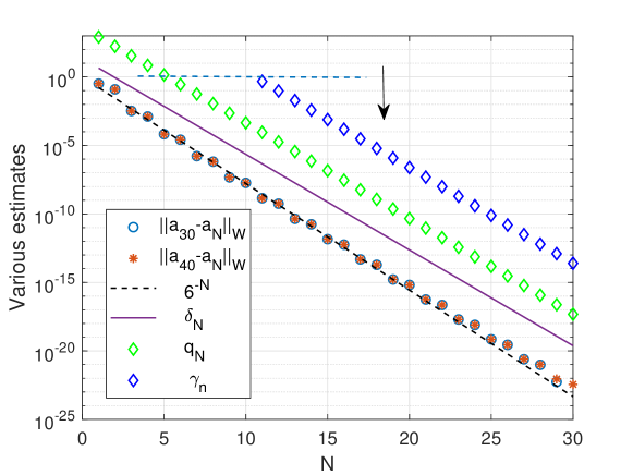
Figure 2: Verification of convergence of the approximation and estimate (42) for Example 6.1.

Note that $\delta_{N}$ is also involved in the estimates of the factors (37), (38). Since the Laurent coefficients of $\alpha_{+}^{(N)}(t)$, $\beta_{-}^{(N)}(t)$ belong the field $\mathbb{Q}(i)$ and $\det a_{N}(t)=1$, the factorisation problem for $a_{N}(t)$ can be solved exactly. We apply the package ExactMPF for solving the factorisation problems for $a_{N}(t)$, $1\leq N\leq 30$.

It turns out that all $a_{N}(t)$ admit the canonical factorisations, which we normalised by the conditions $a_{-}^{(N)}(\infty)=I_{2}$. In Table 1, we also show the values of $\|\bigl{(}a_{\pm}^{(N)}\bigr{)}^{-1}\|_{W}$ and $q_{N}$. For clarity, before to be included into the tables, all exact rational numbers are converted into the floating format preserving their meaningful length.

Starting from $N=6$, the conditions of Theorem 4.1 are fulfilled. Therefore, the matrix functions $a(t)$ and its approximation, $a_{N}(t)$, both admit canonical factorisation.

Since the formulas for factors are cumbersome, we present them in supplementary material.

In Table 2, we also present the values of the right-hand sides of the inequalities (38), (39) denoted by $\delta_{-}^{(N)}$, $\delta_{+}^{(N)}$, respectively. Note that the equality (39) is valid if $\gamma_{N}\leq 1$ (see Corollary 5.1). From Table 1 we see that this condition is fulfilled from $N=11$. Hence we calculate $\delta_{+}^{(N)}$ beginning from $N=11$. They are estimations of the respective norms $\|a_{\pm}^{(N)}-a_{\pm}\|_{W}$. For example, $\|a_{+}-a_{+}^{(15)}\|_{W}<1.275\cdot\,10^{-3}$ and $\|a_{-}-a_{-}^{(15)}\|_{W}<3.490\cdot\,10^{-4}$. In fact, the actual accuracy is much higher. Utilising the same line of reasoning as for the matrix functions above, we present in Figure 3 the norms $\|a_{\pm}^{(40)}-a_{\pm}^{(N)}\|_{W}$ and their estimates $\delta_{\pm}^{(N)}$ for $1\leq N\leq 30$. Again, theoretical estimate for the factors are rather crude in this case.

The respective data are given in Table 2 in Supplementary material, where we also present the norms $\|a_{\pm}^{(N)}-a_{\pm}^{(N-1)}\|_{W}$.

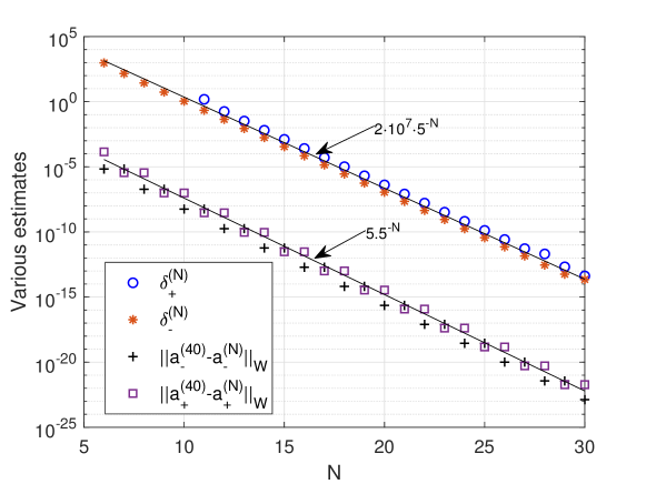
Figure 3: Estimates $\delta_{\pm}^{(N)}$ and the norms $\|a_{\pm}^{(40)}-a_{\pm}^{(N)}\|_{W}$ for Example 6.1.

6.2 Matrix function with equal partial indices, ($\theta=2\nu$).

Now we consider other example.

$$a(t)=\begin{pmatrix}1&\frac{1}{\sqrt{k_{1}^{2}+t^{2}}}\\[8.53581pt] e^{k_{2}t}&t^{2\nu}+\frac{e^{k_{2}t}}{\sqrt{k_{1}^{2}+t^{2}}}\end{pmatrix},\quad 0<k_{1}<1,\quad k_{2}\in\mathbb{C}.$$

Here $\alpha_{+}(t)=e^{k_{2}t}$, $k_{2}\in\mathbb{C}$. It is an entire function, represented by its Taylor series

$$\alpha_{+}(t)=\sum_{n=0}^{\infty}\frac{k_{2}^{n}t^{n}}{n!},$$

and the function $M_{+}$ defined in (18) is $M_{+}(\zeta_{2})=e^{|k_{2}|\zeta_{2}}$, $1<\zeta_{2}<\infty$.

The other function, $\beta_{-}(t)=(k_{1}^{2}+t^{2})^{-1/2}$, $0<k_{1}<1$, with the branch cut $(-k_{1}i,k_{1}i)$ on the imaginary axis, while the branch is fixed by the limiting value $t\beta_{-}(t)\to 1$ as $t=\infty$ is equal to $1$. The function $\beta_{-}(t)$ is analytic into $|t|>k_{1}$ and $\beta_{-}(t)$ is expanded into the series

$$\beta_{-}(t)=\frac{1}{t}\Bigl{(}1+\sum_{n=1}^{\infty}(-1)^{n}\frac{(2n-1)!!}{(2n)!!}\frac{k_{1}^{2n}}{t^{2n}}\Bigr{)},$$

that converges absolutely in the open domain $|t|>k_{1}$. Moreover, $\beta_{-}(t)$, for $|t|=1$, belongs the subalgebra $W_{-}^{0}$. It is easy to prove that $M_{-}(\zeta_{1})=(\zeta_{1}^{2}-k_{1}^{2})^{-1/2}$ for $k_{1}<\zeta_{1}<1$. From (21) we have for $k_{1}<\zeta_{1}<1$, $1<\zeta_{2}<\infty$:

$$\|a-a_{N}\|_{W}\leq\delta_{N}(\zeta_{1},\zeta_{2})=\\ \Biggl{(}1+\frac{\zeta_{2}e^{|k_{2}|\zeta_{2}}}{\zeta_{2}-1}\Biggr{)}\frac{\zeta_{1}^{N+1}}{(1-\zeta_{1})\sqrt{\zeta_{1}^{2}-k_{1}^{2}}}+\Biggl{(}1+\frac{\zeta_{1}}{(1-\zeta_{1})\sqrt{\zeta_{1}^{2}-k_{1}^{2}}}\Biggr{)}\frac{e^{|k_{2}|\zeta_{2}}}{\zeta_{2}^{N}(\zeta_{2}-1)}.$$

Example 6.2.

Let $k_{1}=1/5$, $k_{2}=1$, $\theta=2\nu=6$. Choosing an optimal choice of the parameters $\zeta_{1}$, $\zeta_{2}$, we observed that the pair has small effect on the factorisation process. Thus, we took them basing on the convenience of the numerical calculations.

Numerical experiments lead us to the following values: $\zeta_{1}=1/4$, $\zeta_{2}=4$, and consequently:

$$\delta_{N}=\frac{109e^{4}+60}{27}\frac{1}{\,4^{N}}\approx 222.6364\cdot 4^{-N}.$$ (45)

Similarly to the Example 6.1, we compute the norms $\|a_{30}-a_{N}\|_{W}$, $\|a_{40}-a_{N}\|_{W}$, $\|a_{50}-a_{N}\|_{W}$ and compared them with the calculated values of $\delta_{N}$ for $N\in[1,30]$. The values for $\|a_{50}-a_{N}\|_{W}$ completely coincide with $\|a_{40}-a_{N}\|_{W}$ with the chosen accuracy (DIGID=10). Thus we can assume that the lower bound $\|a_{40}-a_{N}\|_{W}\leq\|a-a_{N}\|_{W}$ is exact and its left hand side fully characterizes the accuracy of the estimate (42). The results are shown in Figure 4 and in the Table 3.

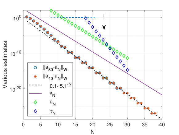
Figure 4: Verification of accuracy of the estimate (42) for Example 6.2.

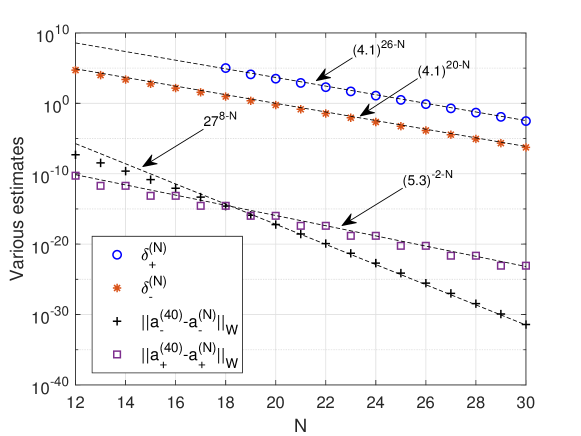
Figure 5: Comparison between $\delta_{\pm}^{(N)}$ with $\|a_{\pm}^{(40)}-a_{\pm}^{(N)}\|_{W}$ for Example 6.2.

As above, the Laurent coefficients of $\alpha_{+}^{(N)}(t)$, $\beta_{-}^{(N)}(t)$ belong the field $\mathbb{Q}(i)$ and $\det a_{N}(t)=1$, hence the factorisation problem for $a_{N}(t)$ can be solved exactly with the package ExactMPF.

It turns out that all $a_{N}(t)$, $3\leq N\leq 30$, admit the stable factorisations with the equal indices $\rho_{1}=\rho_{2}=\nu=3$, in other words, $a_{N}(t)=t^{3}a_{-}^{(N)}(t)a_{+}^{(N)}(t)$. We normalised the factorisations by the conditions $a_{-}^{(N)}(\infty)=I_{2}$. Obviously that estimates (38), (39) hold true in this case.

In Table 3 we show the values of $\|\bigl{(}a_{\pm}^{(N)}\bigr{)}^{-1}\|_{W}$ and $q_{N}(1/4,4)$ (see (23)). From the table we see that starting from $N=12$, the stability criterion is fulfilled. Therefore, the matrix function $a(t)$ admits the stable factorisation with equal indices $\rho_{1}=\rho_{2}=\nu=3$ and the stable factorisation of $a_{N}(t)$ gives an approximate stable factorisation of $a(t)$.

The calculations of the guaranteed accuracy give more or less satisfactory results for $N=30$: $\|a_{+}-a_{+}^{(30)}\|_{W}<3.012\cdot\,10^{-3}$ and $\|a_{-}-a_{-}^{(30)}\|_{W}<5.474\cdot\,10^{-7}$. The values of the norms $\|a_{+}^{(40)}-a_{+}^{(30)}\|_{W}=3.779\cdot\,10^{-32},\|a_{-}^{(40)}-a_{-}^{(30)}\|_{W}=8.741\cdot\,10^{-24}$ show that the actual accuracy is much higher then predicted by the estimate. Comparison $\delta_{\pm}^{(N)}$ with these norms are presented in Figure 5 for all values of $N$ and in the Table 4.

6.3 The stable factorisation of $a(t)$, $\theta=2\nu+1$.

Now we consider the following matrix function

$$a(t)=\begin{pmatrix}1&\frac{e^{k_{1}/t}}{t}\\[5.69054pt] e^{k_{2}t}&t^{\theta}+\frac{e^{k_{1}/t+k_{2}t}}{t}\end{pmatrix},\quad k_{1},k_{2}\in\mathbb{C},\quad\theta=2\nu+1.$$

Here the function $\beta_{-}(t)=t^{-1}e^{k_{1}/t}$ is analytic on $\mathbb{C}\setminus\{0\}$, and $\beta_{-}(\infty)=0$, while $\alpha_{+}(t)=e^{k_{2}t}$ is an entire function. It is easy to check that $M_{-}(\zeta_{1})=\frac{1}{\zeta_{1}}e^{|k_{1}|/\zeta_{1}}$ and $M_{+}(\zeta_{2})=e^{|k_{2}|\zeta_{2}}$, and (21) gives for $0<\zeta_{1}<1$, $1<\zeta_{2}<\infty$:

$$\delta_{N}(\zeta_{1},\zeta_{2})=\Bigl{(}1+\frac{\zeta_{2}e^{|k_{2}|\zeta_{2}}}{\zeta_{2}-1}\Bigr{)}\frac{\zeta_{1}^{N}e^{|k_{1}|/\zeta_{1}}}{1-\zeta_{1}}+\Bigl{(}1+\frac{e^{|k_{1}|/\zeta_{1}}}{1-\zeta_{1}}\Bigr{)}\frac{e^{|k_{2}|\zeta_{2}}}{\zeta_{2}^{N}(\zeta_{2}-1)},$$

In the case of $\theta=2\nu+1$, the stability of the indices occurs at $\rho_{1}=\nu$, $\rho_{2}=\nu+1$. Unfortunately, estimates of the accuracy of the calculation of $\|a_{\pm}-a_{\pm}^{(N)}\|_{W}$ are not available, since the issue of the stability of P-normalisation has not been completed yet.

Example 6.3.

Let $k_{1}=1$, $k_{2}=1/2$, $\theta=-7$, i.e. $\nu=-4$. If we put $\zeta_{1}=1/10$, $\zeta_{2}=10$, then

$$\delta_{N}=\Bigl{(}\frac{10}{9}e^{10}+\frac{110}{81}e^{15}+\frac{1}{9}e^{5}\Bigr{)}\frac{1}{10^{N}}\approx 4.4639\cdot 10^{6-N}.$$

These values of the parameters $\zeta_{1}$, $\zeta_{2}$ give sufficiently small values of $\delta_{N}$ beginning $N=13$ (see Table 5).

Calculations with the package ExactMPF show that for $3\leq N\leq 30$ the matrix functions $a_{N}(t)$ admit the stable factorisations with the indices $\rho_{1}=-4$, $\rho_{2}=-3$. The factorisation constructing by ExactMPF admit $I_{2}$-normalisations starting from $N=4$. We carry out these normalisations by formula (7). Respective estimate in graphical form are presented in Figure 6. Table 5 with the data related to this example is given in the Supplementary Materials.

Then we calculated $\|\bigl{(}a_{\pm}^{(N)}\bigr{)}^{-1}\|_{W}$, and the parameter $q_{N}$ (see Table 5). The criterion $q_{N}<1$ is fulfilled beginning $N=24$. Hence the matrix function $a(t)$ admits the stable factorisation with the indices $\rho_{1}=-4$, $\rho_{2}=-3$.

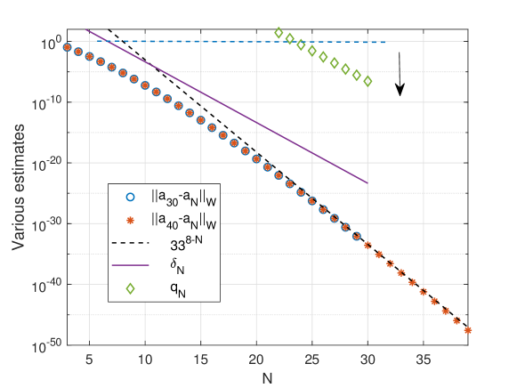
Figure 6: Accuracy of the estimate (42) for Example 6.3.

7 Conclusions

We have developed a method allowing to confidently identify whether a strictly nonsingular $2\times 2$ matrix function possesses stable set of partial indices simultaneously perform an approximate factorisation. For this purpose, we use the ExactMPF package working within the Maple Software environment [18] allowing for exact factorisation of an arbitrary nonsingular polynomial matrix function [19]. We have developed the efficient condition determining the stability region.

Having this crucial information, we have constructed a sequence of polynomial matrix functions approximating the given matrix function in such a way that the distance between the initial matrix function and a consequent member of the approximation sequence decreases, being simultaneously smaller than the stability radius of the respective polynomial matrix function. This, in turn, proves the convergence of the sequence and the stability of the developed factorisation.

The developed approach has been complimented with three different numerical examples demonstrating the method efficiency. We would like to underline, however, that theoretical estimate for the factor approximation in the case where the partial indices are stable but different (Example 6.3) is still to be developed since there are no effective estimates for the radius of neighbourhood where $A$ and $\tilde{A}$ admit the same $P$-normalisation.

Acknowledgements. NA and GM All gratefully acknowledge the support of the EU H2020 grant MSCA RISE- 2020-101008140-EffectFact. GM likes to thank the Isaac Newton Institute for Mathematical Sciences (INI) for their support and hospitality during the programme “Mathematical theory and applications of multiple wave scattering” (MWS), where on this paper was undertaken and supported by EPSRC grant no. EP/R014604/1. GM is also grateful for the funding received from the Simons Foundation that supported their visit to INI during January-June 2023 and participation in MWS programme.

Supplementary material

for the article
A effective criterion for a stable factorisation of a strictly nonsingular $2\times 2$ matrix functions. Utilisation of the ExactMPF package
N. V. Adukova, V. M. Adukov, G. Mishuris

Example 6.1

$N$	$\delta_{N}$	$\|(a_{+}^{(N)})^{-1}\|$	$\|(a_{-}^{(N)})^{-1}\|$	$q_{N}$	$\gamma_{N}$	$\|a_{30}-a_{N}\|_{W}$	$\|a_{40}-a_{N}\|_{W}$
1	4.457	6.000000000	31.00000000	829.021	$3.701\,10^{6}$	$3.252250175\,10^{-1}$	$3.252250175\,10^{-1}$
2	$8.914\,10^{-1}$	6.200000000	31.00000000	171.331	$8.825\,10^{5}$	$1.252650255\,10^{-1}$	$1.252650255\,10^{-1}$
3	$1.783\,10^{-1}$	6.201000600	31.68815767	35.032	$1.845\,10^{5}$	$3.305033488\,10^{-3}$	$3.305033488\,10^{-3}$
4	$3.565\,10^{-2}$	6.213066452	31.68814324	7.020	$3.709\,10^{4}$	$1.285833689\,10^{-3}$	$1.285833689\,10^{-3}$
5	$7.131\,10^{-3}$	6.213066651	31.69452006	1.404	$7.420\,10^{3}$	$6.643388870\,10^{-5}$	$6.643388870\,10^{-5}$
6	$1.426\,10^{-3}$	6.213299946	31.69452005	$2.808\,10^{-1}$	$1.484\,10^{3}$	$2.604989431\,10^{-5}$	$2.604989431\,10^{-5}$
7	$2.852\,10^{-4}$	6.213299946	31.69464756	$5.617\,10^{-2}$	$2.968\,10^{2}$	$1.665819909\,10^{-6}$	$1.665819909\,10^{-6}$
8	$5.705\,10^{-5}$	6.213305778	31.69464756	$1.123\,10^{-2}$	$5.937\,10^{1}$	$6.562780772\,10^{-7}$	$6.562780772\,10^{-7}$
9	$1.141\,10^{-5}$	6.213305778	31.69465074	$2.247\,10^{-3}$	$1.187\,10^{1}$	$4.673619535\,10^{-8}$	$4.673619535\,10^{-8}$
10	$2.282\,10^{-6}$	6.213305942	31.69465074	$4.494\,10^{-4}$	2.375	$1.847014324\,10^{-8}$	$1.847014324\,10^{-8}$
11	$4.564\,10^{-7}$	6.213305942	31.69465083	$8.988\,10^{-5}$	$4.750\,10^{-1}$	$1.404091080\,10^{-9}$	$1.404091080\,10^{-9}$
12	$9.128\,10^{-8}$	6.213305947	31.69465083	$1.797\,10^{-5}$	$9.499\,10^{-2}$	$5.561335285\,10^{-10}$	$5.561335285\,10^{-10}$
13	$1.826\,10^{-8}$	6.213305947	31.69465084	$3.595\,10^{-6}$	$1.890\,10^{-2}$	$4.417597702\,10^{-11}$	$4.417597702\,10^{-11}$
14	$3.651\,10^{-9}$	6.213305947	31.69465084	$7.190\,10^{-7}$	$3.799\,10^{-3}$	$1.752644859\,10^{-11}$	$1.752644859\,10^{-11}$
15	$7.302\,10^{-10}$	6.213305947	31.69465084	$1.438\,10^{-7}$	$7.599\,10^{-4}$	$1.436920153\,10^{-12}$	$1.436920153\,10^{-12}$
16	$1.460\,10^{-10}$	6.213305947	31.69465084	$2.876\,10^{-8}$	$1.520\,10^{-4}$	$5.708247876\,10^{-13}$	$5.708247877\,10^{-13}$
17	$2.921\,10^{-11}$	6.213305947	31.69465084	$5.752\,10^{-9}$	$3.040\,10^{-5}$	$4.792942211\,10^{-14}$	$4.792942215\,10^{-14}$
18	$5.842\,10^{-12}$	6.213305947	31.69465084	$1.150\,10^{-9}$	$6.079\,10^{-6}$	$1.905995816\,10^{-14}$	$1.905995820\,10^{-14}$
19	$1.168\,10^{-12}$	6.213305947	31.69465084	$2.301\,10^{-10}$	$1.216\,10^{-6}$	$1.630494217\,10^{-15}$	$1.630494251\,10^{-15}$
20	$2.337\,10^{-13}$	6.213305947	31.69465084	$4.602\,10^{-11}$	$2.432\,10^{-7}$	$6.489430572\,10^{-16}$	$6.489430919\,10^{-16}$
21	$4.674\,10^{-14}$	6.213305947	31.69465084	$9.204\,10^{-12}$	$4.863\,10^{-8}$	$5.635189764\,10^{-17}$	$5.635193238\,10^{-17}$
22	$9.347\,10^{-15}$	6.213305947	31.69465084	$1.841\,10^{-12}$	$9.723\,10^{-9}$	$2.244407226\,10^{-17}$	$2.244410699\,10^{-17}$
23	$1.869\,10^{-15}$	6.213305947	31.69465084	$3.681\,10^{-13}$	$1.945\,10^{-9}$	$1.973046872\,10^{-18}$	$1.973081604\,10^{-18}$
24	$3.739\,10^{-16}$	6.213305947	31.69465084	$7.363\,10^{-14}$	$3.891\,10^{-10}$	$7.862820339\,10^{-19}$	$7.863167659\,10^{-19}$
25	$7.478\,10^{-17}$	6.213305947	31.69465084	$1.473\,10^{-14}$	$7.782\,10^{-11}$	$6.980519510\,10^{-20}$	$6.983992739\,10^{-20}$
26	$1.495\,10^{-17}$	6.213305947	31.69465084	$2.945\,10^{-15}$	$1.556\,10^{-11}$	$2.781225221\,10^{-20}$	$2.784698451\,10^{-20}$
27	$2.991\,10^{-18}$	6.213305947	31.69465084	$5.890\,10^{-16}$	$3.113\,10^{-12}$	$2.460258627\,10^{-21}$	$2.495001635\,10^{-21}$
28	$5.982\,10^{-19}$	6.213305947	31.69465084	$1.1783\,10^{-16}$	$6.225\,10^{-13}$	$9.605187746\,10^{-22}$	$9.952621710\,10^{-22}$
29	$1.196\,10^{-19}$	6.213305947	31.69465084	$2.356\,10^{-17}$	$1.245\,10^{-13}$	$5.402914661\,10^{-23}$	$8.984270703\,10^{-23}$
30	$2.393\,10^{-20}$	6.213305947	31.69465084	$4.712\,10^{-18}$	$2.490\,10^{-14}$	0	$3.585235396\,10^{-23}$

Table 1: Verification of the criterion $q_{N}<1$ and verification of accuracy of the estimate (42) for Example 6.1.

For example, we have $a(t)\approx a_{-}^{(15)}(t)a_{+}^{(15)}(t)$. All elements of the factor $a_{-}^{(15)}(t)$:

$${\textstyle\bigl{(}a_{-}^{(15)}(t)\bigr{)}_{11}=1.-\frac{5.003000600i}{t}-\frac{0.1000500140\,10^{-1}}{t^{2}}+\frac{0.1000000100i}{t^{3}}+}\\ {\textstyle-\frac{0.1000600220\,10^{-4}}{t^{4}}+\frac{0.9998000600\,10^{-3}i}{t^{5}}-\frac{0.2001300540\,10^{-5}}{t^{6}}+\frac{0.1999400060\,10^{-4}i}{t^{7}}-}\\ {\textstyle\frac{5.003401521\,10^{-8}}{t^{8}}+\frac{4.998200040\,10^{-7}i}{t^{9}}-\frac{1.400980460\,10^{-9}}{t^{10}}+\frac{1.399439988\,10^{-8}i}{t^{11}}-}\\ {\textstyle\frac{4.203000600\,10^{-11}}{t^{12}}+\frac{4.198200768\,10^{-10}i}{t^{13}}-\frac{1.320528106\,10^{-12}}{t^{14}}+\frac{1.320264158\,10^{-11}i}{t^{15}}}.$$

$${\textstyle\bigl{(}a_{-}^{(15)}(t)\bigr{)}_{12}=\frac{1.000200000i}{t}+\frac{0.2000199880\,10^{-2}}{t^{2}}-\frac{0.2000400120\,10^{-1}i}{t^{3}}+}\\ {\textstyle\frac{0.2000399960\,10^{-4}}{t^{4}}-\frac{0.2000400160\,10^{-3}i}{t^{5}}+\frac{4.001000040\,10^{-7}}{t^{6}}-\frac{0.4000800360\,10^{-5}i}{t^{7}}+}\\ {\textstyle\frac{1.000280032\,10^{-8}}{t^{8}}-\frac{1.000200096\,10^{-7}i}{t^{9}}+\frac{2.800840136\,10^{-10}}{t^{10}}-\frac{2.800560280\,10^{-9}i}{t^{11}}+}\\ {\textstyle\frac{8.402638799\,10^{-12}}{t^{12}}-\frac{8.401680864\,10^{-11}i}{t^{13}}+\frac{2.639999789\,10^{-13}}{t^{14}}-\frac{2.640528106\,10^{-12}i}{t^{15}}}$$

$${\textstyle\bigl{(}a_{-}^{(15)}(t)\bigr{)}_{21}=-\frac{25.02500400i}{t}-\frac{0.5001499900\,10^{-1}}{t^{2}}+\frac{0.4999000500i}{t^{3}}-}\\ {\textstyle\frac{0.5000999299\,10^{-3}}{t^{4}}+\frac{0.4997000400\,10^{-2}i}{t^{5}}-\frac{0.1000149790\,10^{-4}}{t^{6}}+\frac{0.9992000700\,10^{-4}}{t^{7}}-}\\ {\textstyle\frac{2.500299359\,10^{-7}}{t^{8}}+\frac{0.2497700160\,10^{-5}i}{t^{9}}-\frac{7.000697979\,10^{-9}}{t^{10}}+\frac{6.993000420\,10^{-8}i}{t^{11}}-}\\ {\textstyle\frac{2.100179772\,10^{-10}}{t^{12}}+\frac{2.097780120\,10^{-9}i}{t^{13}}-\frac{6.602640528\,10^{-12}}{t^{14}}+\frac{6.601320792\,10^{-11}i}{t^{15}}}$$

$${\textstyle\bigl{(}a_{-}^{(15)}(t)\bigr{)}_{22}=1.+\frac{5.003000600i}{t}+\frac{0.9998998599\,10^{-2}}{t^{2}}-\frac{0.9999999800\,10^{-1}i}{t^{3}}+}\\ {\textstyle\frac{0.9997997799\,10^{-4}}{t^{4}}-\frac{0.9997998999\,10^{-3}i}{t^{5}}+\frac{0.1999499460\,10^{-5}}{t^{6}}-\frac{0.1999399700\,10^{-4}i}{t^{7}}+}\\ {\textstyle\frac{4.998598479\,10^{-8}}{t^{8}}-\frac{4.998199079\,10^{-7}i}{t^{9}}+\frac{1.399579540\,10^{-9}}{t^{10}}-\frac{1.399439708\,10^{-8}i}{t^{11}}+}\\ \textstyle{\frac{4.198679400\,10^{-11}}{t^{12}}-\frac{4.198199904\,10^{-10}i}{t^{13}}+\frac{1.319999894\,10^{-12}}{t^{14}}-\frac{1.320264053\,10^{-11}i}{t^{15}}}$$

$N$	$\delta_{+}^{(N)}$	$\delta_{-}^{(N)}$	$\|a_{+}^{(40)}-a_{+}^{(N)}\|$	$\|a_{-}^{(40)}-a_{-}^{(N)}\|$	$\|a_{+}^{(N)}-a_{+}^{(N-1)}\|$	$\|a_{-}^{N}-a_{-}^{(N-1)}\|$
6		948.109	$6.779868266\,10^{-6}$	$1.398370474\,10^{-4}$	$2.673\,10^{-4}$	$5.794\,10^{-9}$
7		144.467	$6.779739474\,10^{-6}$	$3.505946296\,10^{-6}$	$1.537\,10^{-10}$	$1.365\,10^{-4}$
8		27.580	$1.900289452\,10^{-7}$	$3.505944083\,10^{-6}$	$6.684\,10^{-6}$	$3.629\,10^{-12}$
9		5.466	$1.900288549\,10^{-7}$	$9.835458009\,10^{-8}$	$1.075\,10^{-13}$	$3.414\,10^{-6}$
10		1.091	$5.705084618\,10^{-9}$	$9.835457840\,10^{-8}$	$1.871\,10^{-7}$	$2.849\,10^{-15}$
11	1.517	$2.182\,10^{-1}$	$5.705084542\,10^{-9}$	$2.954683944\,10^{-9}$	$9.046\,10^{-17}$	$9.559\,10^{-8}$
12	$1.760\,10^{-1}$	$4.363\,10^{-2}$	$1.794023946\,10^{-10}$	$2.954683942\,10^{-9}$	$5.614\,10^{-9}$	$2.567\,10^{-18}$
13	$3.248\,10^{-2}$	$8.726\,10^{-3}$	$1.794023946\,10^{-10}$	$9.295715063\,10^{-11}$	$8.538\,10^{-20}$	$2.868\,10^{-9}$
14	$6.397\,10^{-3}$	$1.745\,10^{-3}$	$5.833104901\,10^{-12}$	$9.295715063\,10^{-11}$	$1.764\,10^{-10}$	$2.538\,10^{-21}$
15	$1.275\,10^{-3}$	$3.490\,10^{-4}$	$5.833104901\,10^{-12}$	$3.023530855\,10^{-12}$	$8.727\,10^{-23}$	$9.013\,10^{-11}$
16	$2.549\,10^{-4}$	$6.981\,10^{-5}$	$1.945043487\,10^{-13}$	$3.023530855\,10^{-12}$	$5.734\,10^{-12}$	$2.682\,10^{-24}$
17	$5.098\,10^{-5}$	$1.396\,10^{-5}$	$1.945043487\,10^{-13}$	$1.008491079\,10^{-13}$	$9.460\,10^{-26}$	$2.929\,10^{-12}$
18	$1.019\,10^{-5}$	$2.792\,10^{-6}$	$6.615029120\,10^{-15}$	$1.008491079\,10^{-13}$	$1.911\,10^{-13}$	$2.982\,10^{-27}$
19	$2.039\,10^{-6}$	$5.585\,10^{-7}$	$6.615029120\,10^{-15}$	$3.430673589\,10^{-15}$	$1.073\,10^{-28}$	$9.764\,10^{-14}$
20	$4.078\,10^{-7}$	$1.117\,10^{-7}$	$2.285734191\,10^{-16}$	$3.430673589\,10^{-15}$	$6.499\,10^{-15}$	$3.448\,10^{-30}$
21	$8.157\,10^{-8}$	$2.234\,10^{-8}$	$2.285734191\,10^{-16}$	$1.185661780\,10^{-16}$		$3.320\,10^{-15}$
22	$1.631\,10^{-8}$	$4.468\,10^{-9}$	$8.001677628\,10^{-18}$	$1.185661780\,10^{-16}$		$4.116\,10^{-33}$
23	$3.263\,10^{-9}$	$8.937\,10^{-10}$	$8.001677628\,10^{-18}$	$4.151357952\,10^{-18}$		$1.147\,10^{-16}$
24	$6.525\,10^{-10}$	$1.787\,10^{-10}$	$2.831851035\,10^{-19}$	$4.151357952\,10^{-18}$		$5.044\,10^{-36}$
25	$1.305\,10^{-10}$	$3.574\,10^{-11}$	$2.831851035\,10^{-19}$	$1.469410102\,10^{-19}$		$4.014\,10^{-18}$
26	$2.610\,10^{-11}$	$7.148\,10^{-12}$	$1.011526608\,10^{-20}$	$1.469410102\,10^{-19}$		$6.317\,10^{-39}$
27	$5.220\,10^{-12}$	$1.429\,10^{-12}$	$1.011526608\,10^{-20}$	$5.249343203\,10^{-21}$		$1.420\,10^{-19}$
28	$2.044\,10^{-12}$	$2.859\,10^{-13}$	$3.64197255\,10^{-22}$	$5.249343203\,10^{-21}$		$8.059\,10^{-42}$
29	$2.088\,10^{-13}$	$5.719\,10^{-14}$	$3.64197255\,10^{-22}$	$1.890220534\,10^{-22}$		$5.072\,10^{-21}$
30	$4.176\,10^{-14}$	$2.244\,10^{-14}$	$1.320\,10^{-23}$	$1.890220534\,10^{-22}$		$1.045\,10^{-44}$

Table 2: Comparison $\delta_{\pm}^{(N)}$ with $\|a_{\pm}^{(40)}-a_{\pm}^{(N)}\|_{W}$ and the guaranteed accuracy of the approximate canonical factorisation $a(t)\approx a_{-}^{(N)}(t)a_{+}^{(N)}(t)$ for Example 6.1.

Example 6.2

$N$	$\delta_{N}$	$\|(a_{+}^{(N)})^{-1}\|$	$\|(a_{-}^{(N)})^{-1}\|$	$q_{N}$	$\gamma_{N}$	$\|a_{30}-a_{N}\|_{W}$	$\|a_{40}-a_{N}\|_{W}$
1	55.659			333.955	$3.212\,10^{7}$	1.292202089	1.292202089
2	13.915			243.509	$1.859\,10^{8}$	$4.603672092\,10^{-1}$	$4.603672092\,10^{-1}$
3	3.479	13.00000000	26.38888889	1193.388	$2.539\,10^{11}$	$9.653048042\,10^{-2}$	$9.653048042\,10^{-2}$
4	$8.697\,10^{-1}$	28.00539724	43.12791109	1050.407	$1.409\,10^{12}$	$2.075037196\,10^{-2}$	$2.075037196\,10^{-2}$
5	$2.174\,10^{-1}$	106.2638793	193.5327650	4471.338	$2.315\,10^{15}$	$3.112260817\,10^{-2}$	$3.112260817\,10^{-3}$
6	$5.435\,10^{-2}$	106.0198599	193.0173811	1112.297	$1.423\,10^{14}$	$5.052520022\,10^{-4}$	$5.05252002\,10^{-4}$
7	$1.359\,10^{-2}$	106.0270621	193.0175082	278.093	$8.897\,10^{12}$	$5.588691252\,10^{-5}$	$5.588691252\,10^{-5}$
8	$3.397\,10^{-3}$	106.0270621	193.0174816	69.521	$5.560\,10^{11}$	$8.538922599\,10^{-6}$	$8.538922599\,10^{-6}$
9	$8.493\,10^{-4}$	106.0230467	193.0174821	17.380	$3.475\,10^{10}$	$6.805090541\,10^{-7}$	$6.805090541\,10^{-7}$
10	$2.123\,10^{-4}$	106.0230244	193.0174825	4.345	$2.172\,10^{9}$	$1.488151391\,10^{-7}$	$1.488151391\,10^{-7}$
11	$5.308\,10^{-5}$	106.0230225	193.0174825	1.086	$1.357\,10^{8}$	$7.911542747\,10^{-9}$	$7.911542747\,10^{-9}$
12	$1.327\,10^{-5}$	106.0230224	193.0174825	$2.716\,10^{-1}$	$8.484\,10^{6}$	$3.854190119\,10^{-9}$	$3.854190119\,10^{-9}$
13	$3.317\,10^{-6}$	106.0230223	193.0174825	$6.789\,10^{-2}$	$5.303\,10^{5}$	$1.546768305\,10^{-10}$	$1.546768305\,10^{-10}$
14	$8.294\,10^{-7}$	106.0230223	193.0174825	$1.697\,10^{-2}$	$3.314\,10^{4}$	$1.322654352\,10^{-10}$	$1.322654352\,10^{-10}$
15	$2.073\,10^{-7}$	106.0230223	193.0174825	$4.243\,10^{-3}$	$2.071\,10^{3}$	$5.000553058\,10^{-12}$	$5.000553058\,10^{-12}$
16	$5.184\,10^{-8}$	106.0230223	193.0174825	$1.061\,10^{-3}$	$1.295\,10^{2}$	$4.906795682\,10^{-12}$	$4.906795683\,10^{-12}$
17	$1.296\,10^{-8}$	106.0230223	193.0174825	$2.652\,10^{-4}$	8.091	$1.854978316\,10^{-13}$	$1.854978320\,10^{-13}$
18	$3.240\,10^{-9}$	106.0230223	193.0174825	$6.630\,10^{-5}$	$5.057\,10^{-1}$	$1.851904638\,10^{-13}$	$1.851904642\,10^{-13}$
19	$8.099\,10^{-10}$	106.0230223	193.0174825	$1.657\,10^{-5}$	$3.161\,10^{-2}$	$7.038266444\,10^{-15}$	$7.038266829\,10^{-15}$
20	$2.025\,10^{-10}$	106.0230223	193.0174825	$4.144\,10^{-6}$	$1.975\,10^{-3}$	$7.037455514\,10^{-15}$	$7.037455898\,10^{-15}$
21	$5.062\,10^{-11}$	106.0230223	193.0174825	$1.036\,10^{-6}$	$1.235\,10^{-4}$	$2.687290630\,10^{-16}$	$2.687294473\,10^{-16}$
22	$1.265\,10^{-11}$	106.0230223	193.0174825	$2.590\,10^{-7}$	$7.716\,10^{-6}$	$2.687273040\,10^{-16}$	$2.687276884\,10^{-16}$
23	$3.164\,10^{-12}$	106.0230223	193.0174825	$6.475\,10^{-7}$	$4.823\,10^{-7}$	$1.030169742\,10^{-17}$	$1.030208176\,10^{-17}$
24	$7.910\,10^{-13}$	106.0230223	193.0174825	$1.619\,10^{-8}$	$3.014\,10^{-8}$	$1.030169423\,10^{-17}$	$1.030207857\,10^{-17}$
25	$1.977\,10^{-13}$	106.0230223	193.0174825	$4.047\,10^{-9}$	$1.884\,10^{-9}$	$3.958771025\,10^{-19}$	$3.962619441\,10^{-19}$
26	$4.943\,10^{-14}$	106.0230223	193.0174825	$1.012\,10^{-9}$	$1.177\,10^{-10}$	$3.958770976\,10^{-19}$	$3.962619392\,10^{-19}$
27	$1.236\,10^{-14}$	106.0230223	193.0174825	$2.529\,10^{-10}$	$7.359\,10^{-12}$	$1.491648249\,10^{-20}$	$1.528533066\,10^{-20}$
28	$3.090\,10^{-15}$	106.0230223	193.0174825	$6.323\,10^{-11}$	$4.599\,10^{-13}$	$1.491648248\,10^{-20}$	$1.528533066\,10^{-20}$
29	$7.724\,10^{-16}$	106.0230223	193.0174825	$1.581\,10^{-11}$	$2.875\,10^{-14}$	$7.617715140\,10^{-33}$	$5.910646257\,10^{-22}$
30	$1.931\,10^{-16}$	106.0230223	193.0174825	$3.952\,10^{-12}$	$1.797\,10^{-15}$	0	$5.911\,10^{-22}$
31	$4.828\,10^{-17}$						$2.290481164\,10^{-23}$
32	$1.207\,10^{-17}$						$2.290481164\,10^{-23}$
33	$3.017\,10^{-18}$						$8.892504277\,10^{-25}$
34	$7.543\,10^{-19}$						$8.892504277\,10^{-25}$
35	$1.885\,10^{-19}$						$3.455038998\,10^{-26}$
36	$4.714\,10^{-20}$						$3.455038998\,10^{-26}$
37	$1.179\,10^{-20}$						$1.314236521\,10^{-27}$
38	$2.946\,10^{-21}$						$1.314236521\,10^{-27}$
39	$7.366\,10^{-22}$						$2.476508000\,10^{-48}$
40	$1.842\,10^{-22}$						0

Table 3: Verification of the criterion $q_{N}<1$ and verification of accuracy of the estimate (42) for Example 6.2.

$N$	$\delta_{+}^{(N)}$	$\delta_{-}^{(N)}$	$\|a_{+}^{(40)}-a_{+}^{(N)}\|$	$\|a_{-}^{(40)}-a_{-}^{(N)}\|$
12		$5.164\,10^{4}$	$4.878\,10^{-8}$	$5.206370288\,10^{-11}$
13		$1.009\,10^{4}$	$3.494\,10^{-9}$	$1.934759225\,10^{-12}$
14		$2.391\,10^{3}$	$2.334\,10^{-10}$	$1.933162965\,10^{-12}$
15		$5.902\,10^{2}$	$1.462\,10^{-11}$	$7.249988247\,10^{-14}$
16		$1.471\,10^{2}$	$8.617\,10^{-13}$	$7.249964290\,10^{-14}$
17		$3.674\,10^{1}$	$4.795\,10^{-14}$	$2.73906237\,10^{-15}$
18	$1.022\,10^{5}$	9.184	$2.527\,10^{-15}$	$2.739062342\,10^{-15}$
19	$1.305\,10^{4}$	2.296	$1.265\,10^{-16}$	$1.040901891\,10^{-16}$
20	$3.165\,10^{3}$	$5.740\,10^{-1}$	$6.033\,10^{-18}$	$1.040901891\,10^{-16}$
21	$7.898\,10^{2}$	$1.435\,10^{-1}$	$2.745\,10^{-19}$	$3.974538060\,10^{-18}$
22	$1.974\,10^{2}$	$3.587\,10^{-2}$	$1.195\,10^{-20}$	$3.974538060\,10^{-18}$
23	$4.935\,10^{1}$	$8.968\,10^{-3}$	$4.983\,10^{-22}$	$1.523633108\,10^{-19}$
24	$1.234\,10^{1}$	$2.242\,10^{-3}$	$1.995\,10^{-23}$	$1.523633108\,10^{-19}$
25	3.085	$5.605\,10^{-4}$	$7.680\,10^{-25}$	$5.860325899\,10^{-21}$
26	$7.711\,10^{-1}$	$1.401\,10^{-4}$	$2.846\,10^{-26}$	$5.860325899\,10^{-21}$
27	$1.928\,10^{-1}$	$3.503\,10^{-5}$	$1.017\,10^{-27}$	$2.260477723\,10^{-22}$
28	$4.820\,10^{-2}$	$8.758\,10^{-6}$	$3.510\,10^{-29}$	$2.260477723\,10^{-22}$
29	$1.205\,10^{-2}$	$2.189\,10^{-6}$	$1.171\,10^{-30}$	$8.740726716\,10^{-24}$
30	$3.012\,10^{-3}$	$5.474\,10^{-7}$	$3.779\,10^{-32}$	$8.740726716\,10^{-24}$

Table 4: Comparison $\delta_{\pm}^{(N)}$ with $\|a_{\pm}^{(40)}-a_{\pm}^{(N)}\|_{W}$ for Example 6.2.

Example 6.3

$N$	$\delta_{N}$	$\|(a_{+}^{(N)})^{-1}\|$	$\|(a_{-}^{(N)})^{-1}\|$	$q_{N}$	$\|a_{30}-a_{N}\|_{W}$	$\|a_{40}-a_{N}\|_{W}$
1	$4.464\,10^{5}$				2.031	2.031
2	$4.464\,10^{4}$				$5.062\,10^{-1}$	$5.062\,10^{-1}$
3	$4.464\,10^{3}$				$1.095\,10^{-1}$	$1.095\,10^{-1}$
4	446.390	$7.488774053\,10^{5}$	$3.49502\,10^{5}$	$2.337\,10^{14}$	$2.070\,10^{-2}$	$2.070\,10^{-2}$
5	44.639	$9.993003878\,10^{6}$	$4.548002871\,10^{6}$	$4.057\,10^{15}$	$3.366\,10^{-3}$	$3.366\,10^{-3}$
6	4.464	$2.258318561\,10^{7}$	$1.151727289\,10^{7}$	$2.322\,10^{15}$	$4.745\,10^{-4}$	$4.745\,10^{-4}$
7	$4.464\,10^{-1}$	$2.484150034\,10^{8}$	$1.266899999\,10^{8}$	$2.810\,10^{16}$	$5.878\,10^{-5}$	$5.878\,10^{-5}$
8	$4.464\,10^{-2}$	$2.484150037\,10^{8}$	$1.266900000\,10^{8}$	$2.810\,10^{15}$	$6.486\,10^{-6}$	$6.486\,10^{-6}$
9	$4.464\,10^{-3}$	$2.484150037\,10^{8}$	$1.266900000\,10^{8}$	$2.810\,10^{14}$	$6.451\,10^{-7}$	$6.451\,10^{-7}$
10	$4.464\,10^{-4}$	$2.484150037\,10^{8}$	$1.266900000\,10^{8}$	$2.810\,10^{13}$	$5.838\,10^{-8}$	$5.838\,10^{-8}$
11	$4.464\,10^{-5}$	$2.484150037\,10^{8}$	$1.266900000\,10^{8}$	$2.810\,10^{12}$	$4.846\,10^{-9}$	$4.846\,10^{-9}$
12	$4.464\,10^{-6}$	$2.484150037\,10^{8}$	$1.266900000\,10^{8}$	$2.810\,10^{11}$	$3.716\,10^{-10}$	$3.716\,10^{-10}$
13	$4.464\,10^{-7}$	$2.484150037\,10^{8}$	$1.266900000\,10^{8}$	$2.810\,10^{10}$	$2.647\,10^{-11}$	$2.647\,10^{-11}$
14	$4.464\,10^{-8}$	$2.484150037\,10^{8}$	$1.266900000\,10^{8}$	$2.810\,10^{9}$	$1.760\,10^{-12}$	$1.760\,10^{-12}$
15	$4.464\,10^{-9}$	$2.484150037\,10^{8}$	$1.266900000\,10^{8}$	$2.810\,10^{8}$	$1.098\,10^{-13}$	$1.098\,10^{-13}$
16	$4.464\,10^{-10}$	$2.484150037\,10^{8}$	$1.266900000\,10^{8}$	$2.810\,10^{7}$	$6.445\,10^{-15}$	$6.445\,10^{-15}$
17	$4.464\,10^{-11}$	$2.484150037\,10^{8}$	$1.266900000\,10^{8}$	$2.810\,10^{6}$	$3.574\,10^{-16}$	$3.574\,10^{-16}$
18	$4.464\,10^{-12}$	$2.484150037\,10^{8}$	$1.266900000\,10^{8}$	$2.810\,10^{5}$	$1.878\,10^{-17}$	$1.878\,10^{-17}$
19	$4.464\,10^{-13}$	$2.484150037\,10^{8}$	$1.266900000\,10^{8}$	$2.810\,10^{4}$	$9.379\,10^{-19}$	$9.379\,10^{-19}$
20	$4.464\,10^{-14}$	$2.484150037\,10^{8}$	$1.266900000\,10^{8}$	$2.810\,10^{3}$	$4.461\,10^{-20}$	$4.461\,10^{-20}$
21	$4.464\,10^{-15}$	$2.484150037\,10^{8}$	$1.266900000\,10^{8}$	$2.810\,10^{2}$	$2.025\,10^{-21}$	$2.025\,10^{-21}$
22	$4.464\,10^{-16}$	$2.484150037\,10^{8}$	$1.266900000\,10^{8}$	$2.810\,10^{1}$	$8.796\,10^{-23}$	$8.796\,10^{-23}$
23	$4.464\,10^{-17}$	$2.484150037\,10^{8}$	$1.266900000\,10^{8}$	2.810	$3.662\,10^{-24}$	$3.662\,10^{-24}$
24	$4.464\,10^{-18}$	$2.484150037\,10^{8}$	$1.266900000\,10^{8}$	$2.810\,10^{-1}$	$1.463\,10^{-25}$	$1.463\,10^{-25}$
25	$4.464\,10^{-19}$	$2.484150037\,10^{8}$	$1.266900000\,10^{8}$	$2.810\,10^{-2}$	$5.624\,10^{-27}$	$5.624\,10^{-27}$
26	$4.464\,10^{-20}$	$2.484150037\,10^{8}$	$1.266900000\,10^{8}$	$2.810\,10^{-3}$	$2.081\,10^{-28}$	$2.081\,10^{-28}$
27	$4.464\,10^{-21}$	$2.484150037\,10^{8}$	$1.266900000\,10^{8}$	$2.810\,10^{-4}$	$7.428\,10^{-30}$	$7.428\,10^{-30}$
28	$4.464\,10^{-22}$	$2.484150037\,10^{8}$	$1.266900000\,10^{8}$	$2.810\,10^{-5}$	$2.558\,10^{-31}$	$2.560\,10^{-31}$
29	$4.464\,10^{-23}$	$2.484150037\,10^{8}$	$1.266900000\,10^{8}$	$2.810\,10^{-6}$	$8.375\,10^{-33}$	$8.528\,10^{-33}$
30	$4.464\,10^{-24}$	$2.484150037\,10^{8}$	$1.266900000\,10^{8}$	$2.810\,10^{-7}$	0	$2.749\,10^{-34}$
31						$8.586\,10^{-36}$
32						$2.601\,10^{-37}$
33						$7.645\,10^{-39}$
34						$2.183\,10^{-40}$
35						$6.062\,10^{-42}$
36						$1.638\,10^{-43}$
37						$4.308\,10^{-45}$
38						$1.104\,10^{-46}$
39						$2.722\,10^{-48}$
40						0

Table 5: Verification of the criterion $q_{N}<1$ and verification of accuracy of the estimate (42) for Example 6.3.

References

- [1] Gohberg IC, Krein MG. 1958 Systems of integral equations on a half-line with kernels depending on the difference of arguments. Uspekhi Mat. Nauk. 13, 3–72.
- [2] Rogosin S, Mishuris G. 2016 Constructive methods for factorization of matrix-functions. IMA Journal of Applied Mathematics. 81 (2), 365–391. (doi:10.1093/imamat/hxv038)
- [3] Faddeev LD, Takhtajan LA. 2007 Hamiltonian Methods in the Theory of Solitons. Springer, Verlag Berlin: Heidelberg. (doi:10.1007/978-3-540-69969-9)
- [4] Adukov VM, Mishuris G. 2023 Utilisation of the ExactMPF package for solving a discrete analogue of the nonlinear Schrőinger equation by the inverse scattering transform method. Proc. R. Soc. A 479, 20220144. (doi: 10.1098/rspa.2022.0144)
- [5] Litvinchuk GS. 2000 Solvability Theory of Boundary Value Problems and Singular Integral Equations with Shift. Springer, Dordrecht. (doi:10.1007/978-94-011-4363-9)
- [6] Kisil AV, Abrahams ID, Mishuris G, Rogosin SV. 2021 The Wiener–Hopf technique, its generalizations and applications: constructive and approximate methods. Proc. R. Soc. 477, 20210533. (doi:10.1098/rspa.2021.0533)
- [7] Abrahams ID, 1987. Scattering of sound by two parallel semi-infinite screens. Wave Motion. 9 (4), 289–300. (doi:10.1016/0165-2125(87)90002-3)
- [8] Peake N, Abrahams ID. 2020 Sound radiation from a semi-infinite lined duct. Wave Motion. 92, 102407. (doi:10.1016/j.wavemoti.2019.102407)
- [9] Kisil A. 2018 An Iterative Wiener–Hopf Method for Triangular Matrix Functions with Exponential Factors. SIAM Journal on Applied Mathematics. 78, 45–62. (doi:doi.org/10.1137/17M1136304)
- [10] Priddin MJ, Kisil AV, Ayton LJ. 2020 Applying an iterative method numerically to solve matrix Wiener–Hopf equations with exponential factors. Phil. Trans. R. Soc. A 378, 20190241. (doi:10.1098/rsta.2019.0241)
- [11] Clancey KF, Gohberg I. 1981 Factorization of matrix functions and singular integral operators. Operator Theory, Advances and Applications, vol. 3. Basel: Springer.
- [12] Litvinchuk GS, Spitkovsky IM. 1987 Factorization of measurable matrix functions. Basel, Boston: MA: Birkhuser.
- [13] Gohberg IC, Feldman IA. 1974 Convolution equations and projection method for their solution. Amer. Math. Soc. Transl. Math. Monographs 41, Providence, R.I.
- [14] Prssdorf S. 1978 Some classes of singular equations. Series North-Holland Mathematical Library, vol. 17 Amsterdam, the Netherlands; New York, NY: North-Holland Pub. Co.
- [15] Spitkovsky IM. 1974 Stability of partial indices of the Riemann boundary problem with a strictly nonsingular matrix. Doklady Akademii Nauk SSSR. 218, 46–49. (in Russian)
- [16] Adukov V. 1995 On factorization indices of strictly nonsingular matrix function. Integr. Equat. Oper. Th. 21 (1), 1–11.
- [17] Ephremidze L, Spitkovsky I. 2020 On explicit Wiener–Hopf factorization of matrices in a vicinity of a given matrix. Proc. R. Soc. A 476 (2238), 20200027.
- [18] https://www.maplesoft.com/
- [19] Adukov VM, Adukova NV, Mishuris G. 2022 An explicit Wiener-Hopf factorisation algorithm for matrix polynomials and its exact realizations within ExactMPF package. Proc. R. Soc. A 478, 20210941.
- [20] Adukov VM. 1999 On a factorization of analytic matrix-valued functions. Theoretical and Mathematical Physics. 118 (3), 255–263. (doi:10.4213/tmf704)
- [21] Gohberg IC, Lerer L, Rodman L. 1978 Factorization indices for matrix polynomials. Bull. Am. Math. Soc. 84, 275–277. (doi:10.1090/S0002-9904-1978-14473-5)
- [22] Adukov VM. 1992 Wiener–Hopf factorization of meromorphic matrix-valued functions. St. Petersburg Mathematical Journal. 4 (1), 51–69.
- [23] Adukov VM, Mishuris G, Rogosin S. 2020 Exact conditions for preservation of the partial indices of a perturbed triangular matrix function. Proc. R. Soc. A 476, 20200099. (doi:10.1098/rspa.2020.0099)
- [24] Ahlfors LV. 1979 Complex Analysis. McGraw-Hill Book Company, 2 edition.
- [25] Adukov VM. 1998 Generalized inversion of block Toeplitz matrices. Linear Algebra Appl. 274 (1–3), 85–124. (doi:10.1016/S0024-3795(97)00304-2)
- [26] Gohberg IC, Kaashoek MA, Spitkovsky IM. 2003 An overview of matrix factorization theory and operator applications. Operator Theory: Advances and Applications. 141, 1–102.
- [27] Gohberg I, Krupnik N. 1992 One-dimensional Linear Singular Integral Equations. vol. 1. Introduction. Operator theory: Advances and Applications, vol. 53. Birkhiiuser Verlag Basel Boston Berlin. (doi:10.1007/978-94-011-4363-9)
- [28] Mishuris G, Rogosin S. 2014 An asymptotic method of factorization of a class of matrix functions. Proc. R. Soc. A 470, 20140109. (doi:10.1098/rspa.2014.0109)
- [29] Mishuris G, Rogosin S. 2016 Factorization of a class of matrix-functions with stable partial indices. Mathematical Methods in the Applied Sciences. 39 (13), 3791–3807. (doi:10.1002/mma.3825)
- [30] Mishuris G, Rogosin S. 2018 Regular approximate factorization of a class of matrix-function with an unstable set of partial indices. Proceedings of the Royal Society of Edinburgh, Section A: Mathematics. 474 (2209), 0170279. (doi:10.1098/rspa.2017.0279)
- [31] Adukov VM. 2022 Normalization of Wiener–Hopf factorization for matrix functions and its application. Ufa Mathematical Journal. 14 (4), 3–15. (doi:10.13108/2022-14-4-1)
- [32] Adukova NV. 2022 Stability of factorization factors of Wiener–Hopf factorization of matrix functions. Bulletin of the South Ural State University. Series “Mathematics. Mechanics. Physics”. 14 (1), 5–12. (in Russian) (doi:10.14529/mmph220101)
- [33] Adukov VM. 2022 Normalization of Wiener–Hopf factorisation for matrix functions with distinct partial indices. Transactions of A. RazmadzeMathematical Institute. 176 (3), 313–321.
- [34] Adukova NV, Dilman V.L. 2021 Stability of factorization factors of the canonical factorization of Wiener–Hopf matrix functions. Bulletin of the South Ural State University. Series “Mathematics. Mechanics. Physics”. 13 (1), 5–13. (doi:10.14529/mmph210101)