LPSim: Large Scale Multi-GPU Parallel Computing based Regional Scale Traffic Simulation Framework

Abstract

Traffic simulation is a tool for congestion analysis, travel time estimation, and route optimization for urban planning. It is beneficial for navigation apps, transportation network companies, and state agencies. Traditionally, the traffic micro-simulation frameworks are based on road segments and can only support several main roads. Efficient traffic simulation on a regional scale remains a significant challenge due to the complexity of urban mobility and the large scale of spatiotemporal data. This paper introduces a Large Scale Multi-GPU Parallel Computing based Regional Scale Traffic Simulation Framework (LPSim), which is a novel multi-modal regional scale traffic simulation framework that leverages large-scale graphical processing unit (GPU) parallel computing to address these challenges. LPSim utilizes a multi-GPU architecture to simulate extensive and dynamic traffic networks with high fidelity and reduced computation time. Using the parallel processing capabilities of GPUs, LPSim can perform tens of millions of individual vehicle dynamics simulations simultaneously, significantly outperforming traditional CPU-based approaches. The framework is designed to be scalable and can easily accommodate the increasing complexity of traffic simulations. We present the theory behind GPU-based traffic simulation, the architecture of single- and multiple-GPU-based simulations, and the graph partition strategies that optimize computation resource allocation. Our experimental results demonstrate the effectiveness of LPSim in simulating large-scale traffic scenarios. LPSim is capable of completing simulations of 2.82 million trips in merely 6.28 minutes on a single GPU machine equipped with 5120 CUDA cores (Tesla V100-SXM2). Furthermore, utilizing an AWS p2 instance with dual NVIDIA K80 GPUs, which collectively offer 4992 CUDA cores, LPSim successfully simulates 9.01 million trips within 21.45 minutes. This performance not only demonstrates its speed and scalability advantages over traditional simulation techniques but also highlights LPSim’s unique position as the first traffic simulation framework that is adaptable across multi-modal (multiple transportation modes e.g., bikes, subways, and buses) contexts and scalable for both single and multiple GPU configurations. Consequently, LPSim provides an invaluable tool for individuals and extensive research teams alike, enabling the acquisition of large-scale traffic simulation results in a time-efficient manner. LPSim code is available at: https://github.com/Xuan-1998/LPSim

1 Introduction

Traffic simulation, a powerful tool that bridges the areas of computer science and traffic engineering, plays a crucial role in understanding how urban mobility works Zomer et al. [2015]Jiang et al. [2023]. By simulating and recreating traffic scenarios in virtual environments, traffic simulation systems offer a robust platform for researchers, engineers, and policymakers to analyze, experiment, and design strategies to avoid the risks and costs of real-world trials Krautter et al. [1999].

One prevalent approach in traffic simulation is the use of microscopic simulation Treiber et al. [2000] Maroto et al. [2006], which refers to a computer-based modeling technique that simulates the behavior and interactions of individual entities at a microscopic level. In the traffic field, microscopic simulation takes a granular perspective, focusing on individual vehicle movements, accelerations, and lane changes to provide a realistic representation of traffic flow. Compared to macroscopic simulation and mesoscopic simulation, which focus on complete road flow instead of individual vehicle movement Helbing and Molnar [1995], people often use microscopic simulation on the level of cities and highways Maroto et al. [2006] Du et al. [2015], which are smaller scale. However, in recent years, the popularity of large-scale microscopic simulation has grown significantly, driven by the alignment of time-driven microsimulation with the single instruction, multiple data (SIMD) nature of GPU Yedavalli et al. [2021], and the increasing demand for techniques to accommodate various new traffic modes. For example, the Urban Air Mobility (UAM) system Muna et al. [2021] has a regional impact, requiring researchers to evaluate its performance.

Compared with regular-scale microscopic simulation, the aforementioned large-scale microscopic traffic simulation has its challenges. In particular, modeling individual vehicle movements in fine detail, continuously processing, updating the states of numerous individual vehicles, and managing extensive spatiotemporal data in the large-scale microscopic simulation will lead to high computational requirementsAlgers et al. [1997]. Therefore, for practitioners and researchers, large-scale, time-varying simulation data storage and update call for efficient computation tools and a scalable storage approach.

In traffic simulation, the development of GPUs makes it possible to manage the intricate dynamics of vehicle movements and large-scale data structures. Thus, it is possible to utilize the developed GPU architectures to enhance traffic simulation Yedavalli et al. [2022]. In the new traffic simulation framework, LPSim, presented in this paper, we use GPUs to handle both the spatial and temporal aspects of large-scale microscopic traffic simulations. Spatial aspects include the addition or deletion of vehicles, the transfer of vehicle statuses (start, on route, stop) of independent vehicles, and the spatial propagation of the vehicle within the network Barceló et al. [2010]Boxill and Yu [2000]. The temporal dynamics mainly consist of the time propagation and synchronization of traffic flow for each time stepOsorio and Nanduri [2015]. However, the challenge of GPU memory limitations, with a single GPU’s memory capped at 80 GB (for A100) Choquette and Gandhi [2020] and most GPUs have only 8GB memory Zhang et al. [2017], contrasts with the potential for Central Processing Units (CPUs) to scale up to 768 GB (for AWS) Pelle et al. [2019]. To overcome this, our framework employs graph partitioning methods to distribute vast amounts of transportation network and vehicle movement data across multiple GPUs. This strategy ensures that the simulation can scale to accommodate large-scale networks without compromising the level of detail or simulation speed. Our main design innovation for the single GPU framework is summarized in Table 1, and for the multi-GPU system is summarized in Table 2. Based on our research, we claim the contributions in the following four aspects:

• Vectorized Data Storage and Access Implementation: Our approach incorporates vectorized data storage and access mechanisms that allow for the efficient storage and access of both transportation network data and vehicular movement/speed information within a GPU environment. This innovation facilitates improved data handling and processing speed within the GPU architecture.

• Design of the Multi-GPU Transportation Simulation Framework: We have developed a transportation simulation framework that uses multiple GPUs, structured around the concept of graph partitioning. This design ensures the results don’t change as the number of GPUs increases, thereby enhancing the effectiveness and efficiency of the simulation.

• Scalability Benchmarking: The scalability of LPSim has been thoroughly evaluated both theoretically and through empirical research on both one GPU and multiple GPUs. Scalability assessments were conducted using data sourced from the San Francisco County Transportation Authority (SFCTA), complemented by performance analysis based on the Bulk Synchronous Parallel Model Gerbessiotis and Valiant [1994], Amdahl’s law Hill and Marty [2008], and Roofline ModelWilliams et al. [2009], . LPSim demonstrates remarkable efficiency, completing simulations of 2.82 million trips in just 6.28 minutes on a single GPU setup featuring a Tesla V100-SXM2 with 5120 CUDA cores compared with the 12 hours computation time for 0.6 million trips in the same area (San Francisco Bay Area) using CPU-based(conventional) simulation Hsueh et al. [2021], who is simulating less demand but takes longer simulation time and lower simulation fidelity with a mesoscopic simulation approach. Additionally, when the scale becomes larger and has to be deployed on an AWS p2 instance equipped with dual NVIDIA K80 GPUs, which together provide 4992 CUDA cores, LPSim can efficiently simulate 9.01 million trips in a mere 21.45 minutes. These analyses demonstrate the framework’s ability to scale effectively in response to varying computational demands.

• Trade-off between Multi-GPU Parallel Computing and Communication Time: Our investigations reveal that while multi-GPU parallel computing can expedite the simulation process, it is also subject to potential slowdowns due to increased communication times among GPUs. Experiments conducted on systems with 2, 4, and 8 GPUs on a gcloud instance with NVIDIA V100 GPUs have yielded the data, as detailed in Table 3, which is explained further in Section 4.2. It indicates that the increase in the number of GPUs, coupled with appropriate graph partitioning strategies, can lead to a reduction in total computation time required for simulation.

Table 1: SINGLE GPU COMPUTATION DESIGN.

Traffic Data	Structure	Architecture Design
Network	Large scale datab	Contiguous memory blocks Fig 2
Vehicle info	Spatiotemporal data	GPU threads Gupta et al. [2012]$\rightleftharpoons$ vehicles
Agent status Eq. 1	Markov Update	GPU SIMD Yilmazer et al. [2014]

• The network contains more than half a million edges.

Table 2: MULTI-GPU COMPUTATION DESIGN.

Multi GPU challenge	Architecture Design
Multi GPU load balancing	Graph partitioning Fig 4
Inter GPU communication	Ghost zone design Fig 3
Multi GPU synchronization	GPU device based vector Fig 8

The structure of this article is laid out as follows: Section 2 provides some related work of this paper. Section 3 dives into the specifics of our proposed methodology. Following this, Section 4 details the experiments conducted and discusses their outcomes. The performance benchmarking of our approach is then thoroughly examined in Section 4.2. The article is brought to a conclusion in Section 5.

Table 3: Simulation Time /ms

GPU Numbers	2	4	8
Random Partition	Dumped	Dumped	Dumped
Balanced Partition	2498466	1483472	1269893
Unbalance Partition	2014554	1679861	1783668

2 Related Work

2.1 Computational Perspective - From CPU to GPU to multiple GPU

While CPUs have traditionally served as the backbone of general-purpose computing, the emergence of GPUs has triggered a change in processing capabilities. This shift is rooted in the parallel architecture of GPUs, which allows them to simultaneously handle a multitude of tasks. Especially, GPUs excel at SIMD processing Bhandarkar et al. [1996]Franchetti et al. [2005], where a single instruction is executed on multiple data points simultaneously. This is beneficial for tasks involving repetitive and parallelizable computations, such as those found in graphics rendering and scientific simulations. In addition, GPUs feature a high-bandwidth memory hierarchy that allows quick access to large datasets Mei et al. [2014] Mei and Chu [2016]. This is crucial for applications like gaming and data-intensive computations, where rapid access to a vast amount of data is essential for better performance Kim et al. [2011]. As the demands for faster and more efficient processing continue to surge, harnessing the collective power of multiple GPUs is receiving more and more attention. The integration of multiple GPUs represents a substantial advancement, where the collective output transcends the capabilities of individual units with combined memory to enable the scaling to bigger scenarios. This transition not only increases available computational resources but also accelerates the execution of tasks through the synergistic effect to conquer memory constraints Schaa and Kaeli [2009] Stuart and Owens [2011]. However, the integration of multiple GPUs for parallel computing presents a unique set of challenges, which arise from the need to efficiently distribute and synchronize tasks between multiple processors, manage data transfer between GPUs, and address potential bottlenecks of communication and data races. Additionally, software scalability and compatibility become crucial factors, as not all applications can seamlessly leverage the parallel processing capabilities of multiple GPUs Xiao and Feng [2010]. For researchers, navigating the challenges mentioned above is essential for unlocking the full potential of multi-GPU systems and maximizing computational efficiency.

2.2 Traffic Perspective - Simulation Implementation and Framework Design

The aforementioned review of GPUs and multi-GPU computing highlights both advantages and challenges. For general computation missions, addressing such challenges will be difficult and there is no unified framework using multi-GPU computing up to now. In specific research domains, researchers have done works utilizing multi-GPUs in the area of numerical linear algebra Agullo et al. [2011], graph analytics Pan et al. [2017], optimization algorithm solvers Ament et al. [2010], and so on. As far as we know, the use of multiple GPU computations in transportation modeling and simulation tools has not yet achieved widespread adoption. We give a review of the previous simulation strategies in the traffic area first.

Historically, discrete-event simulation and network flow simulation were the standard techniques used in transportation simulation Borgatti [2005]. Their capabilities are further examined in relation to two key functionalities of any transportation simulator: traffic operation Jansen et al. [2004] and dynamic routing Savelsbergh and Sol [1998]. With the advent of multi-modal simulators and the concurrent challenges they posed, agent-based simulation was introduced Railsback et al. [2006]. This approach has a significant impact on the execution speed of the simulations. However, integration of these functions tends to complicate the model, often resulting in slower processing speeds. As functionality becomes more and more complicated, the datasets also become larger and larger.

One solution in transportation to effectively manage large datasets and complicated functions is the use of supercomputers, as Mobiliti Chan et al. [2018] did. Another direction is harnessing the parallel structure of CPU/GPU, as MANTA Yedavalli et al. [2021] uses one GPU in parallel with the CPU to greatly enhance simulation speed. Some traffic simulation software projects, such as BEAM Sheppard et al. [2017] and POLARIS Auld et al. [2016], have also enabled the use of CPU-based parallelism with mesoscopic simulation. The evolution of popular simulations is summarized in Figure 1: We illustrate the simulators’ capabilities with dashed red lines, such as different modes of transportation and dynamic routing of people’s route choices. The dashed blue boundary indicates the growing emphasis on parallelism in recent studies, with some simulators like BEAM, POLARIS, and DTALite focusing on both functionality and parallelism. The arrows depict the evolutionary trajectory of these simulators. For instance, VISSIM, DynaSmart, being proprietary, have led researchers to consider open-source alternatives like SUMO. Aimsun, on the other hand, was developed in response to perceived gaps in SUMO’s analysis and visualization capabilities, despite SUMO’s faster simulation speeds. Moreover, the development of Multi-Agent Transport Simulation (MATSim) signifies a pivotal transition towards agent-based modeling in the transportation sector, diverging from traditional trip-based approaches. This evolution reflects an increasing demand for simulations that can more accurately represent individual behaviors and interactions within transportation networks. Expanding upon MATSim’s foundation, Behavior, Energy, Autonomy, and Mobility (BEAM) introduces enhancements that enable the simulation of electric vehicles, shared mobility services (e.g., bicycles), and the utilization of CPU-based parallelism. The gray boxes signify simulators capable of air traffic simulation, a complex 3D challenge distinct from ground traffic. However, the theory of parallelizable GPU-based traffic simulation and the approach of using multiple GPUs to not only utilize the computation power but also use the added GPU memory to simulate bigger scenarios faster have not been investigated yet.

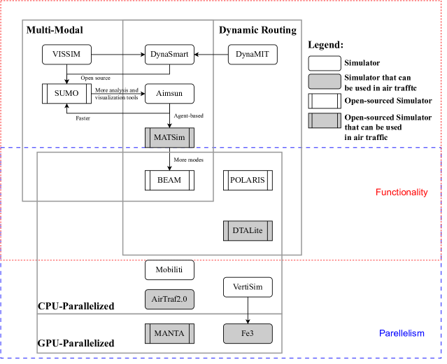
Figure 1: Simulation Evolution Progress Representation Lownes and Machemehl [2006], Mahmassani and Abdelghany [2002], Ben-Akiva et al. [2002], Zhao et al. [2017], Casas et al. [2010], Ronaldo et al. [2012], Behrisch et al. [2011], W Axhausen et al. [2016], Sheppard et al. [2017, 2016], Chan et al. [2018], Yedavalli et al. [2021]

3 Theoretical Analysis of GPU-based traffic simulation

3.1 Basic Components

Table 4: List of Notations for Basic Components 3.1

Symbol	Description	Symbol	Description
$T$	Timestep of the simulation	$S$	Spatial resolution each byte of memory represents
$l_{\text{min}}$	Minimum length of the link of the road network	$v_{i}$	Speed of mode (car, bike, rail, etc.) $i$
$\Delta v$	The velocity difference between a vehicle and the one ahead of it	$\l_{i}(k)$	The location of vehicle $i$ at time step $k$
$u_{i}(k)$	The velocity of vehicle $i$ at time step $k$	$f_{i}$	The function abstraction of IDM car following, lane change, and gap acceptance
$m_{i}$	Probability of a mandatory lane change for vehicle $i$	$x_{i}$	Distance of vehicle $i$ to an exit or intersection
$x_{0}$	Distance of a critical location to the exit or intersection	$g_{\text{lead}}$	Critical lead gap for a lane change
$g_{\text{lag}}$	Critical lag gap for a lane change	$g_{a}$	Desired lead gap for a lane change
$g_{b}$	Desired lag gap for a lane change	$v_{a}$	Speed of the lead vehicle
$v_{b}$	Speed of the lag vehicle	$\alpha_{i}$	Anticipation time of vehicle $i$
$\alpha_{a}$	Anticipation time of the lead vehicle	$\alpha_{b}$	Anticipation time of the lag vehicle
$\epsilon_{a}$	Random component for lead gap	$\epsilon_{b}$	Random component for lag gap
$\dot{v}$	Current acceleration of the vehicle	$a$	Acceleration potential of the vehicle
$v$	Current speed of the vehicle	$v_{o}$	Speed limit of the edge
$\delta$	Acceleration exponent	$s$	Gap between the vehicle and the leading vehicle
$s_{0}$	Minimum spacing between vehicles at a standstill	$b$	Braking deceleration of the vehicle
$T$	Desired time headway

In this part, we introduce the vehicle dynamics used for microsimulation initially developed in Yedavalli et al. [2021]. There are three key components: intelligent driver model, lane change process, and gap acceptance.

We further introduce the concept of Time Step Criteria (TSC) to enhance the model’s adaptability to a multimodal traffic simulation framework. Additionally, we present a theory of parallelizable simulation that aligns with the GPU’s SIMD architecture as shown in Eq. 1. This includes a detailed explanation of how memory is utilized not only to represent the road network but also to depict the occupancy and speed of the vehicles. Lastly, we consolidate our methodology into a comprehensive algorithm, outlined as Algorithm 1. Readers can refer to table 4 for notation in this part.

First, we introduce a set of related notations in Table 4. The dynamics of vehicles within our simulation Treiber and Kesting [2013], is governed by the Intelligent Driver Model (IDM) Albeaik et al. [2022], which models the acceleration of vehicles for updating vehicle locations at each time step. Second, the mandatory lane change process is encapsulated by the formula (Lane Change), as described in Iqbal et al. [2014]. For the vehicle, when the distance to an exit falls below a threshold distance $x_{0}$, it is triggered to make a mandatory lane change and the probability of such a change increases as the vehicle approaches the exit. Once a vehicle inquires for a lane change, it must assess the feasibility of this maneuver by assessing the gaps with both the leading and the lagging vehicles. This assessment is carried out according to the formula (Gap Acceptance), following the guidelines set forth by Choudhury et al. [2007].

$$\dot{v}=a\left(1-\left(\frac{v}{v_{o}}\right)^{\delta}-\left(\frac{s_{o}+Tv+\frac{v\Delta v}{2\sqrt{ab}}}{s}\right)^{2}\right)$$ (IDM)

$$m_{i}=\begin{cases}e^{-\left(x_{i}-x_{0}\right)^{2}}&x_{i}\geq x_{0}\\ 1&x_{i}\textless x_{0}\end{cases}$$ (Lane Change)

$$\begin{cases}\par g_{lead}&=\max\left(g_{a},g_{a}+\alpha_{a}v_{i}+\alpha_{i}\left(v_{i}-v_{a}\right)\right)+\epsilon_{a}\\ g_{lag}&=\max\left(g_{b},g_{b}+\alpha_{i}v_{i}+\alpha_{b}\left(v_{i}-v_{b}\right)\right)+\epsilon_{b}\end{cases}$$ (Gap Acceptance)

Finally, the time step criteria (TSC) means that the relationship between the time step and the spatial resolution needs to be constrained in the following way. For any time step $i$:

$$v_{i}\times T_{tsc}\geq S_{tsc}$$ (TSC-1)

$$V_{i}\times T_{tsc}\leq l_{\text{min}}$$ (TSC-2)

Inequality TSC-1 guarantees that each vehicle advances by at least one cell in every time step. Conversely, inequality (TSC-2) ensures that the distance covered by any vehicle in a single time step does not exceed the length of the shortest link in the road network.

Incorporating the components previously outlined, the traffic simulation process for each subsequent time step is effectively encapsulated by Equation (1). This equation dictates that the position of vehicle $i$ at time step $k+1$ is determined by a specific set of factors: the vehicle’s position and velocity at the preceding time step $k$, the positions of surrounding vehicles at time step $k$, and the speed of the vehicle directly ahead at time step $k$. The computation for each vehicle at time step $k+1$ is conducted independently, relying solely on static data from the previous time step $k$. This approach aligns perfectly with the SIMD architecture of GPUs, enabling efficient parallel processing of traffic simulations.

$$l_{i}(k+1)=f_{i}(\underbrace{l_{i}(k),u_{i}(k)}_{\text{Current Vehicle}},\underbrace{l_{i-n}(k),\ldots,l_{i+n}(k)}_{\text{Surrounding Vehicles}},\underbrace{u_{i+1}(k)}_{\text{Front Vehicle}})$$ (1)

Since $l_{i}(k+1)$ is only dependent on the state in the previous time step $k$, a parallel computation of all vehicle states in time step $k+1$ can be implemented using multiple threads simultaneously. The vehicle propagation process for each vehicle is shown in Algorithm 1.

Remark: One byte can only be occupied by one vehicle, and we are not simulating the case that vehicles crash with each other.

As shown in Figure 2, the whole network will be represented in GPU memory with Char type in C++ which can represent Numbers from 0 to 255, we use it in the following meaning:

• 1 Byte in Memory = 1 Meter in Road Segments

• Value 255 in Memory = Not Occupied by anything in Road Segments

• Value 0-254 = Occupied by Vehicle and the Value is the Speed of the Vehicle in m/s

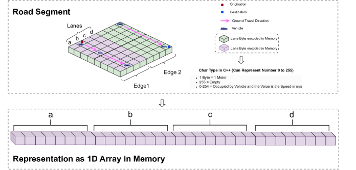
Figure 2: One GPU representation

Algorithm 1 Vehicle Propagation Algorithm

Input: $\mathcal{R}$ (Road Status), $t_{depart}$ (Departure Time), $\mathcal{V}$ (Vehicle Type), $e_{current}$ (Current Edge), $v$ (Speed), $\mathcal{I}$ (Intersection Status)
Parameter: $\Delta t$ (Time Step), $v_{free}$ (Free Flow Speed), $\Theta_{IDM}$ (IDM Parameters $\left(a,\delta,b,s_{0}\right)$ as explained in Table 3.1)
Output: $\mathcal{P}$ (Vehicle Position), $v$ (Speed), $a$ (Acceleration)

1:while Vehicle is active do

2:     if $\mathcal{R}$ is occupied $\lor$ Current Time $<t_{depart}$ then

3:         Wait

4:     else

5:         Start moving

6:         if New edge detected then

7:              $e_{current}\leftarrow$ New Edge ID

8:              $t_{start}\leftarrow$ Current Time

9:              Record $\mathcal{V}$ type

10:              $d_{front}\leftarrow 2\cdot\Delta t\cdot v$          

11:         if Front car within $d_{front}$ then

12:              Update $\mathcal{P},a,v$ using $\Theta_{IDM}$

13:         else

14:              $v\leftarrow v_{free}$          

15:         if Intersection reached then

16:              Proceed according to $\mathcal{I}$’s signal controls

17:         else

18:              Evaluate lane change

19:              if Changing lane then

20:                  if Gap acceptable then

21:                       Change lane                                               

22:return $\mathcal{P},v,a$

3.2 Architecture of single GPU-based traffic simulation

3.2.1 GPU Kernel Design for Vehicle and Traffic Management

In our GPU-based traffic model, the kernel design is a cornerstone of ensuring that the traffic management and vehicle state updates are performed efficiently. Each GPU thread is responsible for updating the state of an individual vehicle and its interaction with the traffic network per simulation time step.

In detail, as shown in the Vehicle Propagation Algorithm 1, the $\mathcal{R}$ Road Status array represents the occupancy status or speed of vehicles on the road, while $\mathcal{I}$ (Intersection Status) denotes the graph nodes. This paper employs an adjacency list to map the directed connectivity of nodes, with list entries pointing to arrays that describe road segments (e.g., a 1D array for a 4-lane, 8-meter road segment will be the dimension of 1 X (4*8), resulting in dimensions of 1 X 32 as shown in Fig 2.) using Char Type in C++ to indicate road status (occupied, empty, and vehicle speed, etc.) , the real road segment is mapped into a 1D array organizing lanes in order. The process begins with each thread checking the road status and vehicle’s departure time to decide whether to depart or wait. Once the vehicle is active, the thread orchestrates the vehicle’s progression, revising its position and velocity in response to the immediate road conditions, such as the presence and distance of preceding vehicles. Additionally, the thread evaluates the vehicle’s interaction with intersections and potential lane changes.

3.2.2 Limitations of Single GPU Architecture and Evolution to Multi-GPU

The limitations of single GPU architectures are notable, particularly in scalability and memory. As traffic simulations grow more complex, a single GPU’s finite cores and bandwidth may lead to longer simulation times. Additionally, the memory limit can constrain the scope of simulatable traffic scenarios.

Multi-GPU framework is an extension of the single GPU architecture, scaling up by distributing the workload across multiple GPUs. This approach inherits the core principles and functionalities of single GPU systems, such as kernel functions and parallel processing, while addressing the performance and memory limitations by enabling larger and more complex traffic simulations.

3.3 Design of multiple GPU-based simulation framework

In scenarios where only a single GPU can be utilized, the entire graph comprising nodes (representing intersections, points of interest, etc.) and edges (depicting the roads or paths between nodes) is stored in one GPU. When multiple GPUs are engaged, the graph is partitioned across these GPUs. This partitioning necessitates an approach to handling the vehicle movements across multiple GPUs. To facilitate this, the graph is divided, and the nodes are distributed across multiple GPUs. Edges that connect nodes situated on different GPUs are placed within a so-called ’ghost zone’, which acts as a replicated buffer area that possesses the same information across the boundaries of adjacent GPUs, ensuring consistency and continuity of information on the network.

In the process of graph partitioning, data are categorized into two types, global data and local data. Global data, which includes the node partitioning scheme (indicating the allocation of specific nodes to particular GPUs) and the complete route of each vehicle, is accessible across all GPUs. Local data such as individual vehicle details in the simulation, the layout of the lanes, intersections, and traffic signal statuses, are stored distinctly within a local GPU.

The propagation of vehicles and the complete road network across multiple GPUs calls for inter-GPU communications to synchronize state and share data. When a vehicle is not located in the ghost zone, the simulator checks whether its next node belongs to the ghost zone. If not, the simulation continues to a single-GPU scenario, eliminating the need for cross-GPU computations. Conversely, if the vehicle is about to enter the ghost zone, it is duplicated in the ghost zone of the destination GPU. If a vehicle is already in a ghost zone, it is assured that its next node is out of the ghost zone which means after the current edge traversal, the vehicle will be on the next GPU and leave the original GPU. At this juncture, it is determined whether the node resides within the current GPU’s domain. If it does, the situation reverts to a single-GPU model as described in Session 3.2 again. If the node is outside the current GPU, the vehicle is marked for removal, and subsequently eliminated post the completion of the simulation timestep. The whole procedure is summarized in Figure 3, intersections within the road network are represented by circles, and we use an adjacency list to illustrate the directed relationships between these intersections. The entries in the list link to the arrays that define road segments. For example, a 4-lane 8-meter road segment is depicted as a 1D matrix with a dimension of 1 x 32 as shown in Fig. 2, showing how real road segments, represented by lines in Fig. 3, are systematically translated into 1D matrices to sequentially organize lanes. In the process of selecting ghost zones, we replicate the entire edge (represented as a 1D array) across both GPUs. To ensure exclusive byte allocation to each vehicle, we transfer vehicles one at a time from one edge to another if the first-byte memory of the downstream edge is not occupied.

By distributing the computation onto different GPUs, our approach allows for scalability and efficient processing of complex simulations that would otherwise be computationally impractical on a single GPU system. We’ll explain the detailed theory and implementation of the above framework in the following subsections.

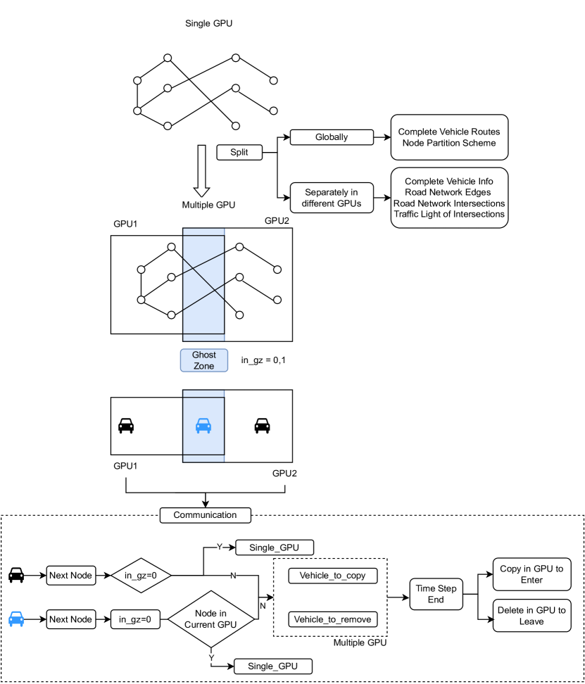
Figure 3: The Framework of the Multi-GPU based traffic simulation

3.3.1 Graph Partitioning

In large-scale multi-GPU parallel simulations, it is essential to distribute graph data across multiple GPUs to share computational resources. We aim for an efficient allocation of extensive graph data, managing computational resources while minimizing inter-GPU communication. In this part, we first state our problem and propose an approximate optimization formulation of the graph partitioning task. Since it is difficult to solve for our network with $200k$ node size, we introduce two applicable graph partitioning strategies to solve the problem. The choice of two graph partitioning methods is closely related to the available computational resources of the single GPU, and the inherent approximation idea of the two methods comes from different perspectives. The framework is summarized as shown in Figure 4, which illustrates that when we have insufficient computational resources, which means that we are creating many more threads than CUDA cores, it leads to a computation-bound scenario. We propose using balanced partitioning to allocate computation evenly across GPUs. On the contrary, with ample computational power, the challenge shifts to minimizing communication overhead, necessitating unbalanced partitioning. Our framework consists of three parts: identifying the difficulties in the partition problem, simplifying it to an optimization formulation, and using efficient algorithms to solve the approximation problem. The left side of Fig. 4 is about modeling the problem, the right side is about how to formulate the problem and solve it, and the middle part is about the detailed components of our solutions.

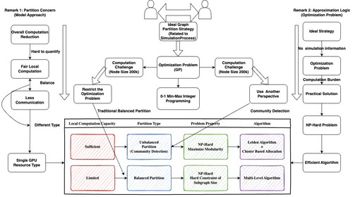
Figure 4: Framework of the graph partitioning strategy

(Optimization Problem of Graph Partitioning) The problem of the GPU partitioning is related to the process of simulation. An ideal partition captures the communications of the multi-GPU system at every time step and seeks to minimize them. However, it relies on the propagation of the simulator and is impossible to achieve before the simulation starts. Below, we formally expressed our optimization formulation based on the route information in the studied time. This optimization problem aims to minimize the calculation in the system under the partition scheme. The optimization is summarized below:

$$\min \quad s$$ (GP)

s.t. $$A_{ij}\cdot\tau_{com}|x_{ik}-x_{jk}|\leq s,\forall i,j,k$$

$$\sum_{i}x_{ik}\leq\overline{l},\ \forall k\in K$$

$$\sum_{k}x_{ik}=1,\ \forall i\in I$$

$$x_{ik}\in\{0,1\},\ \forall i\in I,\forall k\in K$$

In problem GP, we use the following notation: $A_{ij}$ represents the mean number of vehicles that will be travelling from node $i$ to node $j$ within the studied time period. $x_{ik}$ is an indicator variable that takes the value $1$ if node $i$ is in partition $k$, $0$ otherwise. $\tau_{com}$ is the average time needed to communicate then calculate a vehicle between GPUs. $\tau_{cal}$ is the average time needed to calculate a vehicle on a GPU. The set $I$ and $K$ are the sets of graph nodes and the partition indices.

The optimization problem (GP) is $0-1$ min-max integer programming, for which the computational burden will be unaffordable when the graph node size grows to $200k$. This computation issue triggered us to approximate the optimization problem (GP) in different ways.

(Practical Balanced Partition - convert worst case to average) We note that optimization problem GP is optimizing the worse communication case. If we relax the worst case scenario to the average case and add a balanced subgraph size restriction, the problem will be similar to the well-known balanced graph partitioning problem Buluç et al. [2016].

For a specific $(k,1+\varepsilon)$ balanced partition problem, it minimizes the cut, i.e. the total weight of the edges crossing the partitions of $G$ into $k$ components with the size of each component satisfies the constraint below.

$$(1-\varepsilon)\left\lceil\frac{|V|}{k}\right\rceil\leq\left|V_{i}\right|\leq(1+\varepsilon)\left\lceil\frac{|V|}{k}\right\rceil.$$

Typically, balanced graph partitioning problems fall under the category of NP-hard problemsFeldmann and Foschini [2015]. Solutions to these problems are generally derived using heuristics and approximation algorithms. In our work, we use a multi-level graph partitioning algorithmHendrickson et al. [1995]. The key idea of this algorithm is to reduce the size of the graph by collapsing vertices and edges, partitions the smaller graph, then maps back and refines this partition of the original graph.

(Practical Unbalanced Partition - from the community detection perspective) For the balanced graph partitioning stated above, our primary goal is to evenly distribute nodes to each machine, ensuring that no machine possesses an excessively high workload. Simultaneously, we seek to minimize communication between different machines. However, when each GPU has strong computational capabilities, evenly distributing nodes is no longer our primary goal.

In this part, our focus is on effectively identifying community structures in the graph. This involves ensuring tight connections in the communities and sparse connections between communities. We borrow the idea in community detection Fortunato [2010] and propose an unbalanced partition method based on community detection and spatial information. First, by minimizing modularity Newman [2006] through community detection, we obtain $n$ communities with dense internal connections and sparse interconnections. Directly solving the optimal solution in minimizing modularity is hard and time-consuming. Here, we use the Leiden algorithmTraag et al. [2019], which is much faster and yields higher quality solutions. The Leiden algorithm consists of three phases: locally moving nodes, refinement of the partition and aggregation of the network based on the refined partition. For the time complexity, numerical experiments suggest it roughly scales as $O(n)$ or $O(n\log n)$, with $n$ being the number of nodes. Second, utilizing geographical location information, we calculate the central coordinates for each community. We perform $k$-means clustering to the community centre nodes, then we aggregate $n$ communities to $k$ partitions via the result of clustering. (In our experiment, the community number $n$ is much larger than the GPU number $k$)

(Remark: Detailed Explanation of Community Detection) We introduce the concept of modularity and community detection in the following content as the complement of contents above Lancichinetti and Fortunato [2009]Fortunato [2010]Traag et al. [2019]Ahmed et al. [2020].

Modularity is defined as a value in the range $[-1/2,1]$ that measures the density of links inside communities compared to links between communities. For a weighted graph, modularity is defined as:

$$Q=\frac{1}{2m}\sum_{ij}\left[A_{ij}-\frac{k_{i}k_{j}}{2m}\right]\delta\left(c_{i},c_{j}\right)$$

where

• $A_{ij}$ represents the edge weight between nodes $i$ and $j$.

• $k_{i}$ and $k_{j}$ are the sum of the weights of the edges attached to nodes $i$ and $j$, respectively.

• $m$ is the sum of all of the edge weights in the graph.

• $c_{i}$ and $c_{j}$ are the communities of the nodes.

• $\delta$ is Kronecker delta function ( $\delta(x,y)=1$ if $x=y,0$ otherwise).

Based on calculations, the modularity of a community $c$ can be also represented as:

$$Q_{c}=\frac{\Sigma_{in}}{2m}-\left(\frac{\Sigma_{tot}}{2m}\right)^{2}$$

where

• $\Sigma_{in}$ is the sum of edge weights between nodes within the community $c$ (each edge is considered twice)

• $\Sigma_{tot}$ is the sum of all edge weights for nodes within the community (including edges which link to other communities).

(Remark: Implementation Procedure of Graph Partitioning in multi-GPU computation) We will describe how to allocate graph information to multiple GPUs using the graph partitioning method from the previous section.

• Graph Construction: For a fixed time step $t_{k}$, we construct the graph by the vehicle path choice from time step $t_{k}$ to $t_{k+1}$. The vertices and the edges of the graph are cities and roads traveled by cars. The weights of vertices and the edges are related to the number of times they are visited by the vehicle.

• Graph Partitioning: Implement the graph partitioning methods to the graph constructed before.

• Outlier Detection: For those cities never visited in the past time period, we allocate them to the nearest subgraph.

We present an example of partition results for two distinct time periods, showing both balanced and unbalanced graph partitionings in Figures 5 and 6, respectively. These partitions are aligned with the dynamics of the real world traffic flow. Specifically, areas such as the Bay Bridge and Treasure Island are unified within a single cluster due to the incessant flow of traffic in both balanced and unbalanced partition cases because of their heavy traffic throughout the day, underscoring the impracticality of division. In the balanced partition scenario, the map is divided into northern and southern segments by the Bay Bridge area, delineating a clear geographic split. On the other hand, the unbalanced partition strategy, particularly with 4 and 8 clusters, mirrors the Bay Area’s administrative boundaries more closely. For the partition featuring four clusters, the blue, green, and orange parts represent North Bay, East Bay, and South Bay, respectively, while the red segment encompasses the San Francisco and Peninsula areas, along with portions of North and East Bay, interconnected by the Golden Gate Bridge and the Bay Bridge. In the scenario with eight clusters, each segment closely approximates the distinct counties within the Bay Area, with the exception that San Francisco and Marin counties are in one segment.

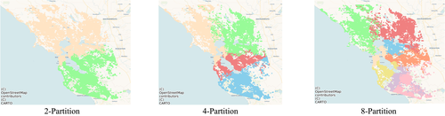
Figure 5: Balanced Graph Partitioning Visualization Based on Half Day Demand

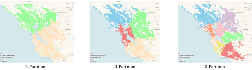
Figure 6: Unbalanced Graph Partitioning Visualization Based on Half Day Demand

3.3.2 Inter-GPU Communication

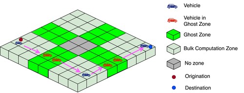
Figure 7: Multiple GPU Representation

The additional cost incurred in a multiple-GPU 7 setup, compared to a single-GPU system, arises predominantly from the need for communication between GPUs. We facilitate communication between multiple GPUs to handle two types of data: vehicles and road networks within ghost zones. Vehicle data transmission occurs when a vehicle enters a ghost zone, while road networks data communication is necessary to maintain consistency across different GPUs when a vehicle moves within a ghost zone. While the use of arrays to store vehicle data, managed via cudaFree and cudaMalloc, presented an intuitive approach, it revealed significant drawbacks, especially in handling variable data sizes. As illustrated in Scenario 1 of Figure 8, allocating excessive memory leads to inefficiency, whereas insufficient allocation, shown in Scenario 2, poses the risk of array index out of bounds. Moreover, this method was hampered by the time-consuming processes involved in frequent memory allocations and deallocations. To efficiently manage the variable-length vehicle data, which needs to be transferred between GPUs, we employ a more effective approach, utilizing device_vector from the Thrust library, the CUDA C++ template library. Thrust’s device_vector is designed for GPU contexts and allows dynamic resizing of its contained elements. This is achieved through efficient memory management strategies, which minimize the overhead of reallocating memory when the device_vector size changes.

Whenever a vehicle is transferred from one GPU to another, we record its original and target data positions. Similarly, when a vehicle needs to be removed from a GPU, we note its data position. A buffer area is designated for tracking vehicles marked for copying or deletion. Each thread responsible for these operations employs atomic operations to identify the buffer position and record the relevant data. This setup facilitates the efficient resizing of the vehicle device_vector and the management of communication data.

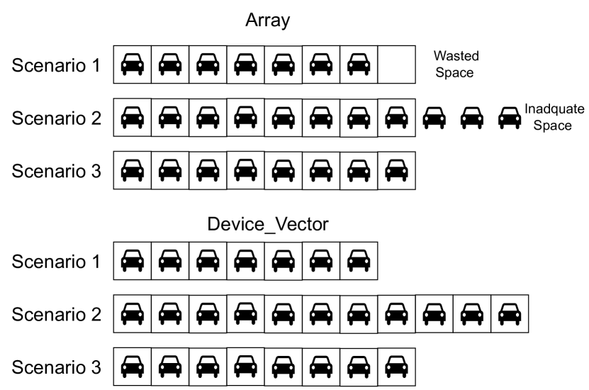
Figure 8: The Advantage of Device_Vector over Array in Storage of Vehicles

As shown in Figure 10, for vehicle replication, threads are launched for each pair of GPUs to handle vehicle data transfer. These threads efficiently employ cudaMemcpyPeer for direct data transfer between GPUs, bypassing the CPU. For vehicle deletions, given the unordered nature of vehicle data storage, the process of data deletion is optimized by moving data from the end of the array to the points of deletion. This method is enhanced through parallel execution across multiple threads, significantly speeding up the deletion process.

Building on the detailed methodologies for vehicle replication and deletion, and road network data consistency, we’ve established a robust system for managing GPU communication. The following section demonstrates the relatively minimal time impact of communication operations compared to read and write processes from one GPU to its local memory, underscoring the practicality and efficiency of our multi-GPU approach. For read and write operations, the cost was assessed by reading and writing large arrays, where each thread manipulates a single array value. In contrast, communication operations were evaluated by replicating a long array from one GPU to another, using both Device-Host-Device (D-H-D) and Peer-to-Peer (P2P) methods. P2P, especially via NVLink, is claimed faster than D-H-D, though its availability depends on the machine’s hardware architecture. Experimental results on V100 GPUs equipped with NVLink revealed that the time cost for P2P communication is approximately threefold that of read-write operations, shown as Figure 9, indicating a reasonably efficient system. In the upcoming performance section, we will elaborate using the example of San Francisco Bay Area, how graph partitioning techniques and other strategies effectively minimize communication overhead to a mere fraction (about 1‰) of the total computational load. In summary, while inter-GPU communication does introduce additional time cost, this is relatively minimal compared to the extensive read and write operations, thereby justifying the use of multiple GPUs for their significant performance benefits.

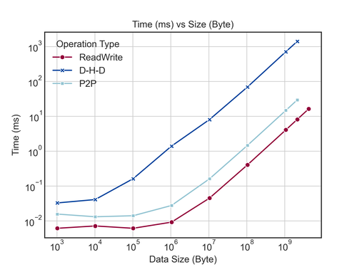
Figure 9: Communication Efficiency

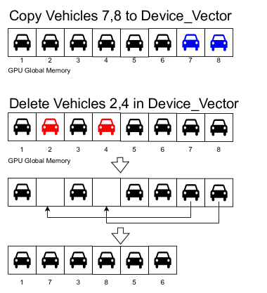
Figure 10: The Method of Vehicle Replication and Deletion

3.4 Scalability Theory of Traffic Simulation

In this section, we propose a way to combine Bulk synchronous parallel (BSP) and normalized runtime across different GPU hardware to measure the scalibility on single-GPU machine. And we also introduced the implications from Amdahl’s law for quantifying the scalibility of multi-GPU traffic simulation

3.4.1 BSP modeling for single-GPU approach performance benchmarking

Currently, the graph computing frameworks largely follow the Bulk Synchronous Parallel (BSP) computation model as shown in figure 11. This model divides computations into a series of iterations called supersteps. The cost of a superstep is the sum of the following three terms:

• Cost of the longest-running local computation

• Cost of global communication between the processors

• Cost of the barrier synchronization at the end of the superstep.

We use the following notations to show the overall computation cost of the BSP model.

• $w_{i}$ - time spent for the local computation in process $i$

• $h_{i}$ - number of messages sent or received by process $i$

• $l$ - time spent for synchronization

The cost of a whole BSP algorithm is the sum of the cost of each superstep: $W+Hg+Sl=\sum_{s=1}^{S}w_{s}+g\sum_{s=1}^{S}h_{s}+Sl$, where $S$ is the number of supersteps.

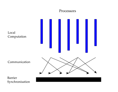
Figure 11: BSP model Cheatham et al. [1996]

3.4.2 Normalizing runtime across different GPU hardware

After introducing the computation model, we consider the normalization of runtime across different GPU hardware, which refers to measuring the runtime in a way that is as independent of hardware specifications as possible. We argue that if the runtime is broken down following the BSP model, it can roughly be normalized using key hardware features. Specifically, we normalize the computation time with the clock rate Bakhoda et al. [2009], the communication time with the bandwidth Pearson et al. [2019], and the synchronization time with bandwidth Zhang et al. [2020]. We will give a brief description below.

For the normalized runtime $\bar{t}_{\mathrm{run}}$, it is given by

$$\bar{t}{\mathrm{run}}=\frac{t{\mathrm{comp}}}{R_{1}/R_{i}}+\frac{t_{\mathrm{comm}}}{B_{1}/B_{i}}+\frac{t_{\mathrm{sync}}}{R_{1}/R_{i}}$$ (2)

Where $R_{i}$ refers to the clock rate in GHz for machine $i$, where $R_{1}$ is the clock rate of the benchmark machine (machine with the lowest number of CUDA cores), and $B_{i}$ refers to the bandwidth in GB/s for the machine $i$, where $B_{1}$ is the bandwidth of the benchmark machine. The number of cores, bandwidth, and the clock rate are independent. The purpose of Equation 2 is to enable a fair comparison across different runs that vary in the number of cores, bandwidth, and clock rates. By normalizing for clock rate and bandwidth, it isolates the measurement of speedup to focus solely on the influence of core count.

3.4.3 An application of Amdahl’s law for multi-GPU scalibility benchmarking

After introducing the single machine computation model, we move to the parallel computing analysis theory in this part. The main tool we want to use is the Amdahl’s law Hill and Marty [2008]. It claims that the theoretical speedup $S_{p}$ that can be achieved with $p$ processors parallelization is

$$S_{p}=\frac{1}{f+\frac{1-f}{p}}$$ (3)

where $f$ refers to the fraction of the computation that must be executed sequentially (i.e., cannot be parallelized), and $1-f$ is the fraction that can be executed in parallel. We note that when $f=0$, $S_{p}=p$ and when $f=1$, $S_{p}=1$.

Another interpretation of the equation (3) is $S_{p}=\frac{t(s,1)}{t(s,p)}$. This equation represents the actual speedup achieved in practice. Here, $t(s,1)$ denotes the sequential runtime of the computation and $t(s,p)$ represents the runtime with $p$ processors.

The equation above shows that as the number of processors increases, the speedup $S_{p}$ of the computation will eventually level off due to the sequential component $f$, which cannot be further parallelized. Therefore, Amdahl’s law suggests that achieving high speedup requires identifying and optimizing the parallelizable parts of a computation while minimizing the sequential components.

To accurately evaluate the performance of a parallel processing system, it is essential to measure the runtime of the computation as a function of the number of processors employed. In the context of parallel algorithms, the evaluation of system performance is a multifaceted task that requires considering various factors such as scalability, communication overhead, load balancing, and problem size. One commonly used approach to assess the efficacy of parallel processing is to compare the run time of the computation for different numbers of processors DeLee [2018], specifically the sequential runtime and the parallel runtime. Sequential runtime denotes the time it takes to execute the portion of the algorithm that cannot be parallelized, while parallel runtime represents the time it takes to execute the portion of the algorithm that can be parallelized.

3.5 Instruction Roofline Model

At the end of this part, we introduce the necessity of the Instruction Roofline Model Ding and Williams [2019], which is an evolution of the Roofline model, to uncover performance bottlenecks and enhance execution efficiency. The Roofline model offers a comprehensive framework for evaluating computing performance by integrating floating point capabilities, arithmetic intensity, and memory bandwidth into a two-dimensional representation. It excels in distinguishing whether a computing task is memory-bound or compute-bound. Ding et al. Ding and Williams [2019] proposed the Instruction Roofline Model for GPUs. Compared with the traditional roofline model, this model shifts the metric to instruction counting, enabling the capture of the mix of floating-point, integer instructions, instruction throughput, and thread predication.

To show the specifics of the Instruction Roofline Model, we draw the picture, in which the warp Instructions per Sector is the x-axis and warp billions of instructions per second (GIPS) is the y-axis. Memory access is coalesced into a sector, which is 32 bytes in size. A warp-level load may trigger between one to 32 sector transactions based on the memory access patterns, making the ”sector” a natural unit for memory access analysis. In the Instruction Roofline Model, the roofline consists of two distinct parts: a horizontal line and sloping lines. The horizontal line embodies the peak performance, which is the maximum warp GIPS achievable by the machine. The sloping lines, on the other hand, reflect the memory bandwidth. The Instruction Roofline Model is described in

$$GIPS\leq\min\left\{\begin{array}[]{l}\text{ Peak GIPS }\\ \text{ Peak GTXN/s }\times\text{ Instruction Intensity }\end{array}\right.$$

where GTXN/s is billions of transactions per second.

For optimal GPU performance within the Roofline Model framework, a program must effectively parallelize by adhering to GPU-specific principles: it should capitalize on data parallelism, optimize memory access for coalescence, reduce warp divergence, enhance arithmetic intensity to favor compute over memory operations, and strategically utilize the GPU’s memory hierarchy to approach the peak GIPS ceiling. These practices ensure that a GPU can perform at its maximum potential, staying within the compute-bound region of the Roofline, indicative of good performance.

4 Experimental Results

4.1 Experimental Data Source

In this study, we engaged in a collaborative effort utilizing data from the San Francisco County Transportation Authority (SFCTA) Bent et al. [2010]. Based on the San Francisco Chained Activity Modeling Process (SF-CHAMP) Outwater and Charlton [2006], a modeling system designed to project transportation patterns across the nine counties of the San Francisco Bay Area. SF-CHAMP 6 leverages observed travel behaviors of San Francisco residents, detailing the socio-economic characteristics and transportation infrastructure of the region to generate key metrics pertinent to transportation and land use planning.

Our analysis focused on a comprehensive dataset encompassing over 19.4 million recorded trips, which is a typical weekday with no significant events or seasonal impactsChan et al. [2023]. Each entry in this dataset was categorized by origin, destination, mode of transportation, and several other critical attributes. A significant portion of our research was devoted to examining car trips, specifically categorized as Single-Occupancy Vehicle (SOV), High Occupancy Vehicle with two occupants (HOV 2), and High Occupancy Vehicle with three or more occupants (HOV 3+). Upon applying these criteria, our scope narrowed down to 15.6 million car trips, constituting 80.4% of the total dataset. This subset provided a substantial basis for analyzing vehicular movement patterns within the region, offering insights into the predominant vechicle propagation and its implications for urban planning and traffic management.

4.2 Experimental Results

We conducted several numerical experiments to showcase the efficacy of our proposed GPU parallel computing based regional scale traffic simulation framework. Specifically, we first demonstrate the result consistency across different number of GPUs used. Next, we tested the random graph partitioning and the proposed balanced/unbalanced partitions, under peak and non-peak hours, which is used to demonstrate the simulation ability under different scenarios of traffic demands, and give us insights on what kind of graph partitioning to be used under what kind of traffic demand scenarios. Finally, we compare the performance of storing vehicles with Device_Vector and array.

To ensure a fair comparison between the random partition and the balanced/unbalanced partition methods, we set the observation range from 0-12 hours for both methods. The computation of the vehicle movement would be affected by different ways of graph partitioning whose departure time is within the observation range.

1) Normalized performance with single-GPU machines having different number of CUDA cores. For this part of the experiment, due to the limitations of GPU memory, the SFCTA demand Bent et al. [2010] cannot be fully processed on a single GPU, and as evidenced in Table 7, careless graph partitioning will also lead to failure. Consequently, we used data from the Bay Area Metropolitan Transportation Commission (MTC) Cox [2013] to model origin-destination demand, specifically concentrating on automobile trips during the morning hours from 5 AM to 12 PM. This includes private vehicles, Transportation Network Companies (TNCs) , and drives to transit stops, excluding public transit and large freight trucks. Although this approach does not perfectly mirror real-world congestion—omitting around 250K trips—it still provides a broad overview with about 3 million trips considered for demonstrating the scalibility of the model .

Table 5: Related Machine Specifications

GPU Name	Tesla M60	Tesla T4	Tesla V100-SXM2
Number of Streaming multiprocessors (SMs)	8	40	80
Core Clock (GHz)	1.18	1.59	1.53
CUDA Cores/SM	256	64	64
Bandwidth (GB/s)	113	215	835
Memory Amount	$8\mathrm{~{}GB}$	16 GB	32 GB
GPU architecture	Maxwell	Turing	Volta
Special Features	dynamic parallelism	real-time ray tracing technology	high-speed communication between GPUs and improved memory bandwidth

Table 6: Normalized runtime on single GPUs

GPU	Number of Cores	Time on Communication (s)	Time on Computation (s)	Time on Synchronization (s)	Total Runtime (s)	Normalized Runtime (s)
Tesla V100-SXM2	5120	36.2192	48.0529	0.7506	85.0227	335.4897992
Tesla T4	2560	139.757	144.854	3.782	288.393	465.9977431
Tesla M60	2048	267.301	377.214	4.405	648.92	648.92

The specifications of the machines used for this study are shown in Table 5. As demonstrated in Figure 12 whose detailed stats is shown in Table 6, the simulation shows a positive correlation between the number of processors used and its overall speedup. However, it should be noted that this increase in speedup is not sustained at the same rate as the initial gains observed with a smaller number of processors Hill and Marty [2008]. As discussed during our discussion in Session 3.4.2, we established that the normalized runtime offers a balanced comparison, assuming that computation, communication, and synchronization times are directly tied to clock rate and bandwidth. However, this analysis did not take into account the architectural variations across different GPUs. This oversight leads to the observation that the Tesla T4 achieves a speedup surpassing the ideal. Despite this, the overarching conclusion indicates that our model benefits from a reduction in execution time as the number of GPUs scales up.

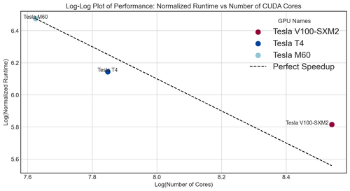
Figure 12: Log-Log Plot of GPU Performance: CUDA Cores vs. Normalized Runtime

2) Performance with different graph partitionings. During the benchmark test, we test 3 different graph partitioning methods with 2, 4, and 8 GPUs, which is shown in Table 7, using gcloud instances with different numbers of V100 GPUs. In order to test the speed of the simulation using different GPUs, we will introduce the notion of ‘Strong Scaling’. Based on Glaser et al. Glaser et al. [2015], in strong scaling, we keep the dataset size (the same demand file in our case) constant but increase the number of processors.

Table 7 demonstrates a reduction in simulation time as the setup scales from 2 to 8 GPUs in a balanced partition, highlighting an enhancement in multi-GPU simulation performance. However, the low speedup observed when transitioning from 4 to 8 GPUs in the balanced scenario suggests that communication becomes a bottleneck in scenarios where the number of GPUs increases without a corresponding enlargement of the problem size, whereas for the unbalanced partition from 4GPUs to 8GPUs, the discrepency of the computations intensity happening in different GPUs becomes a big bottleneck and causes an increase in the simulation time in total.

Table 7: Numerical Results

Simulation Time/ms		2GPUs	4GPUs	8GPUs
Algorithm	Random Partition	Aborted in 80%	Aborted in 80%	Aborted in 80%
	Balanced Partition	2498466	1483472	1269893
	Unbalanced Partition	2014554	1679861	1783668

3) Performance with the adjustment of storing vehicles with Device_Vector. Since we performed an improvement of the data structure from array to Device_Vector, we also conduct a test to compare the performance of the simulation time, and the result is shown below in Table 8. We use a computer with two NVIDIA A100 40GB GPUs to run the test. The result shows that simulation time for storing vehicles with an array is far slower than strong vehicles with a Device_Vector. It is mainly because Device_Vectors usually provide dynamic memory allocation and can be scaled at runtime as needed. Arrays, on the other hand, typically require their size to be determined at compile time. In multi-GPU scenarios, dynamic allocation may allow for more efficient memory usage and better memory allocation policies, reducing memory transfers across GPUs. Using an array also requires large host-to-gpu data transfers rather than Device_Vector storage.

Table 8: Comparison of storing vehicles with Device_Vector over array

		SF bay area 9 counties traffic
Graph Partitioning method		Random	Balanced	Unbalanced
Way of storing	Device_Vector	Aborted	1342463	1287098
	Array	Aborted	70725162	71131945

4) Roofline Model Result. Figure 13 shows the Instruction Roofline applied to NVIDIA’s A100 for our simulator analysis. Blue dots represent non-predicated instructions for each level of the memory hierarchy, highlight the limited data locality, and speedup from sorting. Gold dots are non-predicated loads per global memory access and highlight the loss in near-unit stride access from sorting. The dotted line represents the total (including predicated) instruction throughput. Proximity of blue dots to the highlighted line quantifies the impact of predication. The A100’s architecture, comprising 108 Streaming Multiprocessors (SMs) with four sub-partitions each, integrates a single warp scheduler capable of dispatching one instruction per cycle within each sub-partition. Consequently, the theoretical maximum instruction throughput on a warp basis is calculated as 108×4×1×1.41 GHz, amounting to 609.12 GIPS. We leverage Yang et al.’s methodology Yang et al. [2019] for measuring GPU memory bandwidths but rescale into gigasectors per second (GSECT/s) based on the sector size. We record the number of instructions executed on the thread level, normalized to warp-level by dividing by 32. This instruction count is then divided by the corresponding sector count in data movement to determine the instruction intensity. Performance metrics are calculated by dividing this instruction count by the kernel execution time. The resulting blue markers determined by these calculations fall beneath the sloping roofline, illustrating that the program is memory-bound with room to boost instruction intensity for better performance. Moreover, the disparity between the L1 marker and the L2 and HBM markers underscores efficient L1 data reuse, but not the L2.

Thread predication in GPUs deactivates threads not following a branch, impacting performance by limiting active thread count in a warp. Since a warp processes a single instruction collectively, the fraction of active threads directly influences efficiency. The dotted line in figures represents the maximum warp-level performance, with actual performance falling below this threshold. As is shown in figure 13(a), the dots are well below the dotted line indicating a 10× loss in performance due to thread predication. To address such a significant performance loss, we sorted the input OD pairs by departure time. This approach is depicted in the new roofline results shown in Figure 13(b), where the gap between the performance markers and the theoretical maximum (dotted line) noticeably narrows, reducing the performance loss from a factor of 10 to just 2. This improvement is largely due to the sorting making threads within the same warp more likely to execute similar instructions, significantly reducing the inefficiencies associated with thread predication. For simulations of vehicles within the same area, minimizing the number of instructions is preferable as it leads to reduced resource wastage, thereby accelerating the computation process.

Table 9: Memory Access and Execution Time Before/After Sorting

Version	Load/Store Instruction Count	Sectors Count	Time (s)
Unsorted	5,533,942	14,665,154	195.28
Sorted	830,574	14,547,567	170.75

When a warp accesses global memory, the thread access pattern within that warp is critical, as inefficient memory access patterns can lead to additional, unnecessary transactions, reducing performance. A warp-level load can result in 1 to 32 sector transactions, making the x-axis digit meaningful. A value of 1 indicates ”stride-0” access, where all threads in a warp reference a single memory location, generating only one transaction. On the opposite end, scenarios like random access or striding beyond 32 bytes (”stride-8”) can lead to the maximum 32 transactions, showcasing the spectrum of memory access efficiency. For unit-stride (”stride-1”) access, typical of FP32 or INT32 operations, the global load/store (LD/ST) intensity stands at 1/4. Our model lies between stride-1 and stride-0 which is indicating a good global memory access pattern of our model. However, as illustrated with the gold dots in Figure 13(b), the sorted version reveals a deterioration in the memory access pattern. This observation is supported by the statistics of instruction count and sector numbers presented in Table 9. After sorting, the total number of instructions decreased, yet the number of sectors accessed decreased only slightly. This discrepancy suggests that the compiler optimizations may have optimized away many instructions in the sorted program. It is important to emphasize that the Roofline model, while useful, should be considered a supplementary tool that benefits from being paired with runtime and scalability analysis. In our case, despite the memory access pattern requiring further improvement, the reduction in execution time post-sorting confirms the beneficial impact of sorting.

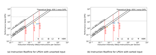
Figure 13: The Instruction Roofline for our simulator.

5 Conclusion

This paper introduces LPSim, a cutting-edge traffic simulation framework that leverages multi-GPU computation for enhanced performance and efficiency. Unlike traditional traffic simulation models, LPSim integrates graph partitioning methods tailored for multi-GPU environments, ensuring a near-optimal resource utilization and faster processing times.

A key innovation of LPSim is its multi-GPU computation strategy, which allocates graph information across multiple GPUs and manages the spatio-temporal data efficiently. This approach accelerates the computation of the system, allowing for the simulation of more complex and larger traffic networks than the previous work. The communication component of LPSim, especially in multi-GPU setups, is carefully designed to handle vehicle movements across different GPUs, ensuring data consistency and simulation reliability.

The experimental results, validated against real-world data, demonstrate LPSim’s superior accuracy in replicating traffic dynamics. The framework’s performance analysis reveals significant advantages in using multiple GPUs over a single GPU setup, including scalability and efficiency in handling large-scale traffic simulations.

Future enhancements of LPSim are threefold.

Firstly, from the multimodal perspective, we will focus on extending its capabilities to multimodal traffic scenarios, further bridging the gap between theoretical traffic models and practical traffic management applications. This will deepen our understanding of complex routing challenges within simulations, paving the way for more comprehensive and accurate traffic modeling. Although we have not tested the multimodal systems on LPSim, we have gotten the bike network from Open Street Map Map [2014], and the SFCTA data Bent et al. [2010] we have provides the bike mode. We plan to use these datasets to test multimodal systems in the future. This progressive approach will help in the field of traffic simulation and smarter management, contributing to smarter, more responsive urban planning strategies.

Secondly, from the theoretical design and analysis perspective, we are passionate about capturing the dynamics of the simulation system and designing a more efficient graph partitioning strategy. And we’ll explore the possibility of using shared memory for better data locality to improve modal. The computation model given in this paper will be further explored. In addition to refining the model, more detailed calibration and routing algorithms are crucial for analyzing real-world results. Our team is actively investigating the application of dynamic traffic rerouting strategies. To ensure the accuracy and validity of our model, we will leverage Uber movement data Sun et al. [2020] for calibration and validation purposes.

Thirdly, acknowledging the inefficiencies of storing vehicle and road network information in global memory, we consider partitioning each GPU into multiple segments, wherein related data would be stored in shared memory. This approach is anticipated to facilitate faster data retrieval and processing, as shared memory access times are comparable to those of the L1 cache, thereby potentially reducing the latency associated with global memory access. However, this strategy introduces the potential for additional computational and communication overhead. We plan to rigorously evaluate the trade-offs between improved data access speeds and the increased complexity of managing shared memory spaces.

In the end, the framework’s user-friendly design, with a one-click Docker setup, makes it accessible to a broad range of users, from researchers to urban planners. The open-source nature of LPSim not only highlights its potential for broad adoption but also invites ongoing enhancements and innovations from the global community. Looking ahead, there are plans to integrate LPSim into a variety of practical applications, notably in urban traffic management and the development of smart cities. This integration is poised to significantly enhance the efficiency and sustainability of urban infrastructures.

References

- Agullo et al. [2011] Agullo, E., Augonnet, C., Dongarra, J., Faverge, M., Ltaief, H., Thibault, S., Tomov, S., 2011. Qr factorization on a multicore node enhanced with multiple gpu accelerators, in: 2011 IEEE International Parallel & Distributed Processing Symposium, IEEE. pp. 932–943.
- Ahmed et al. [2020] Ahmed, M., Seraj, R., Islam, S.M.S., 2020. The k-means algorithm: A comprehensive survey and performance evaluation. Electronics 9, 1295.
- Albeaik et al. [2022] Albeaik, S., Bayen, A., Chiri, M.T., Gong, X., Hayat, A., Kardous, N., Keimer, A., McQuade, S.T., Piccoli, B., You, Y., 2022. Limitations and improvements of the intelligent driver model (idm). SIAM Journal on Applied Dynamical Systems 21, 1862–1892.
- Algers et al. [1997] Algers, S., Bernauer, E., Boero, M., Breheret, L., Di Taranto, C., Dougherty, M., Fox, K., Gabard, J.F., 1997. Review of micro-simulation models. Review Report of the SMARTEST project .
- Ament et al. [2010] Ament, M., Knittel, G., Weiskopf, D., Strasser, W., 2010. A parallel preconditioned conjugate gradient solver for the poisson problem on a multi-gpu platform, in: 2010 18th Euromicro Conference on Parallel, Distributed and Network-based Processing, IEEE. pp. 583–592.
- Auld et al. [2016] Auld, J., Hope, M., Ley, H., Sokolov, V., Xu, B., Zhang, K., 2016. Polaris: Agent-based modeling framework development and implementation for integrated travel demand and network and operations simulations. Transportation Research Part C: Emerging Technologies 64, 101–116.
- Bakhoda et al. [2009] Bakhoda, A., Yuan, G.L., Fung, W.W., Wong, H., Aamodt, T.M., 2009. Analyzing cuda workloads using a detailed gpu simulator, in: 2009 IEEE international symposium on performance analysis of systems and software, IEEE. pp. 163–174.
- Barceló et al. [2010] Barceló, J., et al., 2010. Fundamentals of traffic simulation. volume 145. Springer.
- Behrisch et al. [2011] Behrisch, M., Bieker, L., Erdmann, J., Krajzewicz, D., 2011. Sumo–simulation of urban mobility: an overview, in: Proceedings of SIMUL 2011, The Third International Conference on Advances in System Simulation, ThinkMind.
- Ben-Akiva et al. [2002] Ben-Akiva, M., Bierlaire, M., Koutsopoulos, H.N., Mishalani, R., 2002. Real time simulation of traffic demand-supply interactions within dynamit, in: Transportation and network analysis: current trends. Springer, pp. 19–36.
- Bent et al. [2010] Bent, E., Koehler, J., Erhardt, G., 2010. Evaluating regional pricing strategies in san francisco–application of the sfcta activity-based regional pricing model, in: 89th Annual Meeting of the Transportation Research Board, Washington, DC.
- Bhandarkar et al. [1996] Bhandarkar, S.M., Chirravuri, S., Arnold, J., 1996. Parallel computing of physical maps—a comparative study in simd and mimd parallelism. Journal of computational biology 3, 503–528.
- Borgatti [2005] Borgatti, S.P., 2005. Centrality and network flow. Social networks 27, 55–71.
- Boxill and Yu [2000] Boxill, S.A., Yu, L., 2000. An evaluation of traffic simulation models for supporting its. Houston, TX: Development Centre for Transportation Training and Research, Texas Southern University .
- Buluç et al. [2016] Buluç, A., Meyerhenke, H., Safro, I., Sanders, P., Schulz, C., 2016. Recent advances in graph partitioning. Springer.
- Casas et al. [2010] Casas, J., Ferrer, J.L., Garcia, D., Perarnau, J., Torday, A., 2010. Traffic simulation with aimsun, in: Fundamentals of traffic simulation. Springer, pp. 173–232.
- Chan et al. [2023] Chan, C., Kuncheria, A., Macfarlane, J., 2023. Simulating the impact of dynamic rerouting on metropolitan-scale traffic systems. ACM Transactions on Modeling and Computer Simulation 33, 1–29.
- Chan et al. [2018] Chan, C., Wang, B., Bachan, J., Macfarlane, J., 2018. Mobiliti: Scalable transportation simulation using high-performance parallel computing, in: 2018 21st International Conference on Intelligent Transportation Systems (ITSC), IEEE. pp. 634–641.
- Cheatham et al. [1996] Cheatham, T., Fahmy, A., Stefanescu, D., Valiant, L., 1996. Bulk synchronous parallel computing—a paradigm for transportable software. Tools and Environments for Parallel and Distributed Systems , 61–76.
- Choquette and Gandhi [2020] Choquette, J., Gandhi, W., 2020. Nvidia a100 gpu: Performance & innovation for gpu computing, in: 2020 IEEE Hot Chips 32 Symposium (HCS), IEEE Computer Society. pp. 1–43.
- Choudhury et al. [2007] Choudhury, C.F., Ben-Akiva, M.E., Toledo, T., Lee, G., Rao, A., 2007. Modeling cooperative lane changing and forced merging behavior, in: 86th Annual Meeting of the Transportation Research Board, Washington, DC.
- Cox [2013] Cox, W., 2013. Plan bay area .
- DeLee [2018] DeLee, E., 2018. Assessing the scalability of parallel programs: Case studies from ibamr .
- Ding and Williams [2019] Ding, N., Williams, S., 2019. An instruction roofline model for gpus. IEEE.
- Du et al. [2015] Du, Y., Zhao, C., Zhang, X., Sun, L., 2015. Microscopic simulation evaluation method on access traffic operation. Simulation Modelling Practice and Theory 53, 139–148.
- Feldmann and Foschini [2015] Feldmann, A.E., Foschini, L., 2015. Balanced partitions of trees and applications. Algorithmica 71, 354–376.
- Fortunato [2010] Fortunato, S., 2010. Community detection in graphs. Physics reports 486, 75–174.
- Franchetti et al. [2005] Franchetti, F., Kral, S., Lorenz, J., Ueberhuber, C.W., 2005. Efficient utilization of simd extensions. Proceedings of the IEEE 93, 409–425.
- Gerbessiotis and Valiant [1994] Gerbessiotis, A.V., Valiant, L.G., 1994. Direct bulk-synchronous parallel algorithms. Journal of parallel and distributed computing 22, 251–267.
- Glaser et al. [2015] Glaser, J., Nguyen, T.D., Anderson, J.A., Lui, P., Spiga, F., Millan, J.A., Morse, D.C., Glotzer, S.C., 2015. Strong scaling of general-purpose molecular dynamics simulations on gpus. Computer Physics Communications 192, 97–107. URL: https://www.sciencedirect.com/science/article/pii/S0010465515000867, doi:https://doi.org/10.1016/j.cpc.2015.02.028.
- Gupta et al. [2012] Gupta, K., Stuart, J.A., Owens, J.D., 2012. A study of persistent threads style GPU programming for GPGPU workloads. IEEE.
- Helbing and Molnar [1995] Helbing, D., Molnar, P., 1995. Social force model for pedestrian dynamics. Physical review E 51, 4282.
- Hendrickson et al. [1995] Hendrickson, B., Leland, R.W., et al., 1995. A multi-level algorithm for partitioning graphs. SC 95, 1–14.
- Hill and Marty [2008] Hill, M.D., Marty, M.R., 2008. Amdahl’s law in the multicore era. Computer 41, 33–38.
- Hsueh et al. [2021] Hsueh, G., Czerwinski, D., Poliziani, C., Becker, T., Hughes, A., Chen, P., Benn, M., 2021. Using beam software to simulate the introduction of on-demand, automated, and electric shuttles for last mile connectivity in santa clara county .
- Iqbal et al. [2014] Iqbal, M.S., Choudhury, C.F., Wang, P., González, M.C., 2014. Development of origin–destination matrices using mobile phone call data. Transportation Research Part C: Emerging Technologies 40, 63–74.
- Jansen et al. [2004] Jansen, B., Swinkels, P.C., Teeuwen, G.J., de Fluiter, B.v.A., Fleuren, H.A., 2004. Operational planning of a large-scale multi-modal transportation system. European Journal of Operational Research 156, 41–53.
- Jiang et al. [2023] Jiang, X., Tang, Y., Tang, Z., Cao, J., Bulusu, V., Poliziani, C., Sengupta, R., 2023. Simulating the integration of urban air mobility into existing transportation systems: A survey. arXiv preprint arXiv:2301.12901 .
- Kim et al. [2011] Kim, J., Kim, H., Lee, J.H., Lee, J., 2011. Achieving a single compute device image in opencl for multiple gpus. ACM Sigplan Notices 46, 277–288.
- Krautter et al. [1999] Krautter, W., Manstetten, D., Schwab, T., 1999. Traffic simulation for the development of traffic management systems, in: Traffic and Mobility: Simulation—Economics—Environment, Springer. pp. 193–204.
- Lancichinetti and Fortunato [2009] Lancichinetti, A., Fortunato, S., 2009. Community detection algorithms: a comparative analysis. Physical review E 80, 056117.
- Lownes and Machemehl [2006] Lownes, N.E., Machemehl, R.B., 2006. Vissim: a multi-parameter sensitivity analysis, in: Proceedings of the 2006 Winter Simulation Conference, IEEE. pp. 1406–1413.
- Mahmassani and Abdelghany [2002] Mahmassani, H.S., Abdelghany, K.F., 2002. Dynasmart-ip: Dynamic traffic assignment meso-simulator for intermodal networks, in: Advanced modeling for transit operations and service planning. Emerald Group Publishing Limited, pp. 200–229.
- Map [2014] Map, O.S., 2014. Open street map. Online: https://www. openstreetmap. org. Search in .
- Maroto et al. [2006] Maroto, J., Delso, E., Felez, J., Cabanellas, J.M., 2006. Real-time traffic simulation with a microscopic model. IEEE Transactions on Intelligent Transportation Systems 7, 513–527.
- Mei and Chu [2016] Mei, X., Chu, X., 2016. Dissecting gpu memory hierarchy through microbenchmarking. IEEE Transactions on Parallel and Distributed Systems 28, 72–86.
- Mei et al. [2014] Mei, X., Zhao, K., Liu, C., Chu, X., 2014. Benchmarking the memory hierarchy of modern gpus, in: Network and Parallel Computing: 11th IFIP WG 10.3 International Conference, NPC 2014, Ilan, Taiwan, September 18-20, 2014. Proceedings 11, Springer. pp. 144–156.
- Muna et al. [2021] Muna, S.I., Mukherjee, S., Namuduri, K., Compere, M., Akbas, M.I., Molnár, P., Subramanian, R., 2021. Air corridors: Concept, design, simulation, and rules of engagement. Sensors 21, 7536.
- Newman [2006] Newman, M.E., 2006. Modularity and community structure in networks. Proceedings of the national academy of sciences 103, 8577–8582.
- Osorio and Nanduri [2015] Osorio, C., Nanduri, K., 2015. Energy-efficient urban traffic management: a microscopic simulation-based approach. Transportation Science 49, 637–651.
- Outwater and Charlton [2006] Outwater, M.L., Charlton, B., 2006. The san francisco model in practice. Innovations in Travel Demand Modeling 24.
- Pan et al. [2017] Pan, Y., Wang, Y., Wu, Y., Yang, C., Owens, J.D., 2017. Multi-gpu graph analytics, in: 2017 IEEE International Parallel and Distributed Processing Symposium (IPDPS), IEEE. pp. 479–490.
- Pearson et al. [2019] Pearson, C., Dakkak, A., Hashash, S., Li, C., Chung, I.H., Xiong, J., Hwu, W.M., 2019. Evaluating characteristics of cuda communication primitives on high-bandwidth interconnects, in: Proceedings of the 2019 ACM/SPEC International Conference on Performance Engineering, pp. 209–218.
- Pelle et al. [2019] Pelle, I., Czentye, J., Dóka, J., Sonkoly, B., 2019. Towards latency sensitive cloud native applications: A performance study on aws, in: 2019 IEEE 12th International Conference on Cloud Computing (CLOUD), IEEE. pp. 272–280.
- Railsback et al. [2006] Railsback, S.F., Lytinen, S.L., Jackson, S.K., 2006. Agent-based simulation platforms: Review and development recommendations. Simulation 82, 609–623.
- Ronaldo et al. [2012] Ronaldo, A., et al., 2012. Comparison of the two micro-simulation software aimsun & sumo for highway traffic modelling.
- Savelsbergh and Sol [1998] Savelsbergh, M., Sol, M., 1998. Drive: Dynamic routing of independent vehicles. Operations Research 46, 474–490.
- Schaa and Kaeli [2009] Schaa, D., Kaeli, D., 2009. Exploring the multiple-gpu design space, in: 2009 IEEE International Symposium on Parallel & Distributed Processing, IEEE. pp. 1–12.
- Sheppard et al. [2017] Sheppard, C., Waraich, R., Campbell, A., Pozdnukov, A., Gopal, A.R., 2017. Modeling plug-in electric vehicle charging demand with BEAM: The framework for behavior energy autonomy mobility. Technical Report. Lawrence Berkeley National Lab.(LBNL), Berkeley, CA (United States).
- Sheppard et al. [2016] Sheppard, C.J., Harris, A., Gopal, A.R., 2016. Cost-effective siting of electric vehicle charging infrastructure with agent-based modeling. IEEE Transactions on Transportation Electrification 2, 174–189.
- Stuart and Owens [2011] Stuart, J.A., Owens, J.D., 2011. Multi-gpu mapreduce on gpu clusters, in: 2011 IEEE International Parallel & Distributed Processing Symposium, IEEE. pp. 1068–1079.
- Sun et al. [2020] Sun, Y., Ren, Y., Sun, X., 2020. Uber movement data: A proxy for average one-way commuting times by car. ISPRS International Journal of Geo-Information 9, 184.
- Traag et al. [2019] Traag, V.A., Waltman, L., Van Eck, N.J., 2019. From louvain to leiden: guaranteeing well-connected communities. Scientific reports 9, 5233.
- Treiber et al. [2000] Treiber, M., Hennecke, A., Helbing, D., 2000. Microscopic simulation of congested traffic, in: Traffic and Granular Flow’99: Social, Traffic, and Granular Dynamics, Springer. pp. 365–376.
- Treiber and Kesting [2013] Treiber, M., Kesting, A., 2013. Traffic flow dynamics. Traffic Flow Dynamics: Data, Models and Simulation, Springer-Verlag Berlin Heidelberg , 983–1000.
- W Axhausen et al. [2016] W Axhausen, K., Horni, A., Nagel, K., 2016. The multi-agent transport simulation MATSim. Ubiquity Press.
- Williams et al. [2009] Williams, S., Waterman, A., Patterson, D., 2009. Roofline: an insightful visual performance model for multicore architectures. Communications of the ACM 52, 65–76.
- Xiao and Feng [2010] Xiao, S., Feng, W.c., 2010. Inter-block gpu communication via fast barrier synchronization, in: 2010 IEEE International Symposium on Parallel & Distributed Processing (IPDPS), IEEE. pp. 1–12.
- Yang et al. [2019] Yang, C., Kurth, T., Williams, S., 2019. Hierarchical roofline analysis for gpus: Accelerating performance optimization for the nersc‐9 perlmutter system. Concurrency and Computation: Practice and Experience 32. URL: https://api.semanticscholar.org/CorpusID:160018817.
- Yedavalli et al. [2021] Yedavalli, P., Kumar, K., Waddell, P., 2021. Microsimulation analysis for network traffic assignment (manta) at metropolitan-scale for agile transportation planning. Transportmetrica A: Transport Science , 1–22.
- Yedavalli et al. [2022] Yedavalli, P., Kumar, K., Waddell, P., 2022. Microsimulation analysis for network traffic assignment (manta) at metropolitan-scale for agile transportation planning. Transportmetrica A: Transport Science 18, 1278–1299.
- Yilmazer et al. [2014] Yilmazer, A., Chen, Z., Kaeli, D., 2014. Scalar waving: Improving the efficiency of simd execution on gpus, in: 2014 IEEE 28th International Parallel and Distributed Processing Symposium, IEEE. pp. 103–112.
- Zhang et al. [2017] Zhang, H., Si, S., Hsieh, C.J., 2017. Gpu-acceleration for large-scale tree boosting. arXiv preprint arXiv:1706.08359 .
- Zhang et al. [2020] Zhang, L., Wahib, M., Zhang, H., Matsuoka, S., 2020. A study of single and multi-device synchronization methods in nvidia gpus, in: 2020 IEEE International Parallel and Distributed Processing Symposium (IPDPS), IEEE. pp. 483–493.
- Zhao et al. [2017] Zhao, X., Wan, C., Sun, H., Xie, D., Gao, Z., 2017. Dynamic rerouting behavior and its impact on dynamic traffic patterns. IEEE Transactions on Intelligent Transportation Systems 18, 2763–2779.
- Zomer et al. [2015] Zomer, L.B., Moustaid, E., Meijer, S., 2015. A meta-model for including social behavior and data into smart city management simulations, in: 2015 Winter Simulation Conference (WSC), IEEE. pp. 1705–1716.