Words Worth a Thousand Pictures: Measuring and Understanding Perceptual Variability in Text-to-Image Generation

Abstract

Diffusion models are the state of the art in text-to-image generation, but their perceptual variability remains understudied. In this paper, we examine how prompts affect image variability in black-box diffusion-based models. We propose W1KP, a human-calibrated measure of variability in a set of images, bootstrapped from existing image-pair perceptual distances. Current datasets do not cover recent diffusion models, thus we curate three test sets for evaluation. Our best perceptual distance outperforms nine baselines by up to 18 points in accuracy, and our calibration matches graded human judgements 78% of the time. Using W1KP, we study prompt reusability and show that Imagen prompts can be reused for 10–50 random seeds before new images become too similar to already generated images, while Stable Diffusion XL and DALL-E 3 can be reused 50–200 times. Lastly, we analyze 56 linguistic features of real prompts, finding that the prompt’s length, CLIP embedding norm, concreteness, and word senses influence variability most. As far as we are aware, we are the first to analyze diffusion variability from a visuolinguistic perspective. Our project page is at http://w1kp.com.

1 Introduction

In text-to-image generation, pictures are worth a thousand words, but which words are worth a thousand pictures? Specifically, how do prompts affect perceptual variation in generated imagery across random seeds? Consider these prompts:

1. A matte orange ball in the center against a pure white background.

2. Orange ball against white background.

As shown in Figure 1, the first conveys a single particular illustration, while the second elicits multiple interpretations. Orange could refer to the fruit or the color, and the scene geometry is underspecified. But how can we quantify and characterize these linguistic intuitions?

In this paper, we study the connection between visual variability and language in black-box text-to-image models, focusing on state-of-the-art diffusion models. Previous work tends to study the perceptual distance Zhang et al. (2018) between pairs of images, while a prompt can generate a near infinite set of images. Furthermore, previous approaches have not been explicitly calibrated for human-friendly grades of similarity. What does a score of, for example, 0.2 mean in terms of perceived similarity? Such calibration is likely crucial for robust human interpretation.

Figure 1: DALL-E 3 images for the prompts “a matte orange ball in the center against a pure white background” (top) and “orange ball against white background” (bottom). Our W1KP score quantifies the perceptual similarity for each set of images. It yields 0.99 and 0.68 for the top and bottom rows, showing the greater image variability of the latter.

To bridge these gaps in the literature, we first propose a straightforward framework for constructing human-calibrated perceptual variability measures based on existing perceptual distance metrics. We call it the Words of a Thousand Pictures method, or W1KP ([’wIk.pi:]) for short. On our crowd-sourced dataset of human-judged images from DALL-E 3, Imagen, and Stable Diffusion XL (SDXL), we validate our choice of DreamSim Fu et al. (2024), a recent distance trained on Stable Diffusion Rombach et al. (2022) images. Our variant of DreamSim outperforms the best baseline by 0.1–0.4 points in two-alternative forced choice and 0.2–0.4 points in accuracy. To improve interpretability, we normalize and calibrate scores to graded human judgements on four levels of perceptual similarity, with cutoff points corresponding to high (0.85–1.0), medium (0.4–0.85), low (0.2–0.4), and no similarity ($<$0.2), which yield a correct classification 78% of the time.

Next, to ground our academic discourse, we investigate the practical implications of our approach. Suppose a computer graphics practitioner wishes to generate a diverse array of images from a single prompt, but it is unclear how much it can be reused with different seeds before additional images contribute little to the variability of the overall set of images. Our work provides a quantitative metric for prompt reusability, as we explore further in Section 4.1. On DiffusionDB Wang et al. (2023), an open dataset of user-written text-to-image prompts, we find that the same prompt can be reused for Imagen for 10–20 random seeds, while SDXL and DALL-E 3 are more reusable at 100–200 seeds.

Finally, we study how 56 linguistic features affect generation variability. Although research has explored optimizing for image variability in diffusion Sadat et al. (2024), they have not investigated the contributing linguistic constructs. To understand the underlying structure of these 56 features, we perform an exploratory factor analysis over DiffusionDB and uncover four factors of keyword presence (e.g., “dog walking, 4K, watercolor”), syntactic complexity (e.g., Yngve depth), linguistic unit length, and semantic richness. Then, we conduct clean-room, single-word generation experiments over the three strongest features in the semantic richness factor (concreteness, CLIP embedding norm, and number of word senses) to assess their contribution more precisely. We confirm that all three linguistic features significantly ($p<0.01$) correlate with perceptual variability for all three diffusion models studied.

Our contributions are as follows: (1) we propose and validate a human-calibrated framework for building perceptual variability metrics from existing perceptual distance metrics; (2) we examine a new practical application of the method in assessing prompt reusability in text-to-image generation; and (3) we provide original insight into the linguistic sources of variability in diffusion models, finding that keywords, syntactic complexity, length, and semantic richness influence variability.

2 Our W1KP Approach

2.1 Preliminaries

Text-to-image diffusion models are a family of denoising generative models broadly consisting of two components: a text encoder that produces latent representations of language, such as T5 Raffel et al. (2020) or CLIP Radford et al. (2021), and a denoising image decoder that transforms random noise into an image conditioned on text, e.g., a convolutional variational auto-encoder (VAE; Rombach et al., 2022). To generate an image, we feed a prompt into the text encoder, pass its representation to the image decoder along with randomly sampled noise, then iteratively denoise the noise into a meaningful image. Large-scale models are generally trained using score matching Song et al. (2021) on billions of image–caption pairs Podell et al. (2024), such as the now-deprecated LAION-5B dataset Schuhmann et al. (2022).

To conduct a general study, we explore diffusion in a black-box manner to be able to generalize to proprietary models. Formally, let a text-to-image model be $G(\{w_{i}\};s,\bm{\theta})$ whose codomain comprises the sample space of all images $\mathcal{I}$ and domain the sequence of words $\{w_{i}\}$, random seed $s\in\mathbb{Z}$ to initialize the image noise, and learned parameters $\bm{\theta}\in\mathbb{R}^{p}$. To generate multiple images from a single prompt, a standard practice is to run multiple trials for different random seeds $s$ Podell et al. (2024), which we follow in our experiments.

Our analyses target three state-of-the-art models, one open and two proprietary:

1. Stable Diffusion XL Podell et al. (2024), an open model which uses CLIP Radford et al. (2021) for encoding text and a 2.6 billion-parameter U-Net Ronneberger et al. (2015) for generating images.

2. DALL-E 3 Betker et al. (2023), a proprietary API from OpenAI incorporating a pretrained T5-XXL Raffel et al. (2020) text encoder and the same image decoder architecture as SDXL.

3. Imagen Saharia et al. (2022), a similarly proprietary API from Google using a T5-XXL encoder and an efficient variant of a similar convolutional U-Net decoder.

All models produce images at least 1024$\times$1024 pixels in resolution. Further details about the three models can be found in Appendix A.2.

2.2 Our General Framework

We aim to measure the visual variability of a set of synthetic images. Toward this, we propose to aggregate perceptual distances, which are well studied in the literature, among all pairs of images in a set. To aid human interpretation of the distances, we apply two steps: first, normalization, which squashes potentially unbounded and “odd” distributions into the standard uniform distribution $U[0,1]$. For instance, a perceptual distance with a tight range of 5.10–5.19 across 1,000 image sets would be difficult to comprehend. Second, we calibrate the distances to graded human judgements of similarity and determine the corresponding cutoff points, giving meaning to score ranges (see Figure 3).

Concretely, let $\bm{I}:=\{I_{i}\}_{i=1}^{n}\subseteq\mathcal{I}$ be an i.i.d. sample of images generated by $G(\cdot)$. We seek a function $\eta(\bm{I})$ such that $\eta(\bm{I}^{\prime})<\eta(\bm{I})$ if $\bm{I}^{\prime}$ is more self-similar than $\bm{I}$ is. A starting point is perceptual distance, a symmetric $\delta:\mathcal{I}\times\mathcal{I}\mapsto\mathbb{R}^{+}$ that assigns larger values to less similar image pairs. Many metrics Fu et al. (2024) embed $I_{a},I_{b}\in\mathcal{I}$ using a feature extractor $f:\mathcal{I}\mapsto\mathbb{R}^{\ell}$, such as ViT Dosovitskiy et al. (2021), then compute a distance $d:\mathbb{R}^{\ell}\times\mathbb{R}^{\ell}\mapsto\mathbb{R}^{+}$ between $f(I_{a})$ and $f(I_{b})$, e.g., Euclidean distance. To standardize these distances to $U[0,1]$ for better interpretability, we apply the cumulative distribution function transform, defined as $F(x):=\mathbb{P}(X\leq x)$. It has the property of $F(X)$ being uniformly distributed:

Proposition 2.1.

If $X$ is a continuous random variable, $F(X)$ is standard uniform $U[0,1]$.

Hence, a normalized $d^{*}$ is

$$d^{*}(I_{a},I_{b}):=F(d(f(I_{a}),f(I_{b}))),$$ (1)

and $F$ is estimated from a sample $\{d(I_{a_{i}},I_{b_{i}})\}_{i=1}^{m}$ as $\hat{F}(d(I_{a},I_{b})):=|\{d(I_{a_{i}},I_{b_{i}})\leq d(I_{a},I_{b}):1\leq i\leq m\}|/m$. As our sample, we generate 10,000 image pairs per diffusion model for 1,000 randomly selected DiffusionDB prompts.

Equipped with a uniform perceptual distance, we now construct measures of image set variability ($\eta$). A natural framework to do this is to define a family of $U$-statistics Li (2012); Hoeffding (1948) over sets of images:

Definition 2.1.

Let $h:\mathbb{R^{\ell}}\times\cdots\times\mathbb{R}^{\ell}\mapsto\mathbb{R}^{+}$ be an $\alpha$-arity kernel parameterized by $d$. Then a family of $U$-statistics for measuring image set variability can be defined as

$$U_{d,h}(\bm{I}):=\frac{1}{\binom{n}{\alpha}}\sum_{1\leq i_{1}<\cdots<i_{\alpha}\leq n}h(f(I_{i_{1}}),\dots,f(I_{i_{\alpha}});d).$$ (2)

Certain choices of $h$ produce estimators of interest. We use two in our experiments:

• Pairwise mean ($\eta_{\text{mean}})$: let $d=d^{*}$, $\alpha=2$, and $h(\bm{x},\bm{y};d)=d(\bm{x},\bm{y})$. This measures the expected similarity among all pairs of images.

• $k$-expected maximum ($\eta_{k}$): let $d=d^{*}$, $\alpha=k$, and $h(\bm{x}_{1},\dots,\bm{x}_{\alpha})=\min\{d(\bm{x}_{i},\bm{x}_{j}):i\neq j\}$. This quantifies the expected maximum similarity between a pair of images in a set of size $k$.

We note a connection to statistical dispersion: if $d$ is the squared Euclidean distance and $h$ the pairwise mean kernel, $U_{d,h}$ is proportional to the trace of the covariance matrix of $f(I_{1}),\dots,f(I_{n})$, i.e., the total variance. A proof is in Appendix B. Furthermore, to match the convention of scores in $[0,1]$ denoting similarity rather than dissimilarity (e.g., $R^{2}$), for the rest of this paper we invert $\eta$ and report $\tilde{\eta}:=1-\eta$ instead, calling it the W1KP score.

Figure 2: An illustration of W1KP: image embeddings (see A) and pairwise distances (B) computed using a backbone model, fed into the normalization function (C; Eqn. 1) producing a single score in $[0,1]$. The calibration module (D; Eqn. 3) aligned to human judgements (E) then assigns a similarity level (F).

Lastly, we find cutoff points for $\tilde{\eta}$ calibrated to human-judged levels of high, medium, low, and no similarity. For the human judgement data, we gather a dataset $\{(I_{x_{i}},I_{y_{i}},z_{i})\}_{i=1}^{N}$, where $I_{x_{i}},I_{y_{i}}\in\mathcal{I}$ are a pair of generated images from the same prompt, and $z_{i}\in\{\text{none},\text{low},\text{mid},\text{high}\}$ is the human-annotated level of similarity between $I_{x_{i}}$ and $I_{y_{i}}$ (see Section 3.2 for details). On the dataset, we optimize the cutoff points $\beta_{\text{low}}<\beta_{\text{mid}}<\beta_{\text{high}}$ to maximize the label accuracy of the splits $S_{\text{none}}:=[0,\beta_{\text{low}})$, $S_{\text{low}}:=[\beta_{\text{low}},\beta_{\text{mid}})$, $S_{\text{mid}}:=[\beta_{\text{mid}},\beta_{\text{high}})$, $S_{\text{high}}:=[\beta_{\text{high}},1.0]$:

$$\operatorname*{argmax}_{\beta_{\text{low}},\beta_{\text{mid}},\beta_{\text{high}}}\frac{1}{N}\sum_{i=1}^{N}\mathbb{I}(\tilde{\eta}(\{I_{x_{i}},I_{y_{i}}\})\in S_{z_{i}}),$$ (3)

where $\mathbb{I}$ is the indicator function. We illustrate our overall method in Figure 2, and a proof of Proposition 2.1 is given in Appendix B.

3 Veracity Analyses

Before applying W1KP, we first verify the quality of the perceptual distance backbone and interpretability of the score on human judgements.

3.1 W1KP Quality

Method	SDXL		Imagen		DALL-E 3
	2AFC	Acc.	2AFC	Acc.	2AFC	Acc.
Oracle	80.0	100	80.7	100	79.3	100
L2	54.8	55.4	61.0	63.3	58.5	60.1
SSIM	55.2	56.7	59.1	61.7	57.6	59.3
LPIPS	64.7	68.6	67.6	72.0	64.8	70.8
ST-LPIPS	60.0	62.4	63.4	67.6	59.6	65.4
DISTS	65.5	69.4	67.5	71.9	63.7	67.5
SSCD (Large)	63.4	66.7	66.0	69.1	63.3	66.7
CoPer (CLIPB32)	63.2	67.8	64.4	68.9	62.4	67.9
Raw (CLIPL14)	67.3	72.4	70.3	76.3	67.3	75.0
DreamSim (Orig.)	69.2	75.0	71.3	77.3	70.3	77.9
DreamSim${}_{\ell_{2}}$ (Ours)	69.3	75.2	71.5	77.5	70.7	78.3

Table 1: Quality of the backbones on our evaluation sets, across the image generation model.

Setup. Following prior work in perceptual distance evaluation Zhang et al. (2018), we crowd-sourced a dataset of two-alternative forced-choice (2AFC) image triplets using Amazon MTurk Hauser and Schwarz (2016). Five unique workers were shown three generated images from the same prompt—a reference image, image A, and image B—and instructed to pick whether A or B resembled the reference more. This was repeated three times each for 500 random prompts from DiffusionDB, a large dataset of user-written prompts, for each of SDXL, Imagen, and DALL-E 3, totaling 1,500 triplets per model. Formally, let $\{(I_{r_{i}},I_{a_{i}},I_{b_{i}},y_{a_{i}})\}_{i=1}^{M}$ be a dataset of $M$ triplets, where $I_{r_{i}},I_{a_{i}},I_{b_{i}}\in\mathcal{I}$ are images and $y_{a_{i}}\in\{0,\dots,5\}$ the number of workers choosing $I_{a_{i}}$ over $I_{b_{i}}$. We used attention checks throughout the process; for more details, see Appendix A.3.

For our non-neural methods, we evaluated raw-image Euclidean distance (L2) and the structural similarity index (SSIM; Wang et al., 2004). For our neural backbones, we tested the popular LPIPS Zhang et al. (2018), its shift-tolerant variant ST-LPIPS Ghildyal and Liu (2022), and an SSIM-inspired variant DISTS Ding et al. (2020), all based on VGG-16 Simonyan and Zisserman (2015); SSCD Pizzi et al. (2022), a model trained for image copy detection; CoPer Li et al. (2022), an extension of LPIPS to ViT; raw cosine similarity from CLIP; and lastly, DreamSim Fu et al. (2024), which ensembles pretrained transformers trained on Stable Diffusion images for feature extraction and applies cosine distance for measurement. Since DreamSim’s domain was closest to ours, we hypothesized that it would be most effective. We also evaluated our variant, DreamSim${}_{\ell_{2}}$, with L2 instead of cosine distance for $d$, which benefits from being a true mathematical distance and hence allows for multidimensional scaling analyses, as in Appendix E.

We used the standard evaluation metrics of 2AFC score, defined as the mean proportion of workers agreeing with the backbone’s scores, i.e., $\frac{1}{M}\sum_{i=1}^{M}\mathbb{I}(I_{a_{i}}\succ_{r}I_{b_{i}})\frac{y_{a_{i}}}{5}+\mathbb{I}(I_{a_{i}}\prec_{r}I_{b_{i}})(1-\frac{y_{a_{i}}}{5})$, where $I_{a_{i}}\prec_{r}I_{b_{i}}$ if $\tilde{\eta}(\{I_{r_{i}},I_{a_{i}}\})<\tilde{\eta}(\{I_{r_{i}},I_{b_{i}}\})$, and majority-vote accuracy. We let $\tilde{\eta}=\tilde{\eta}_{\text{mean}}$. See Appendix A.3 for further setup details.

Results. We present our results in Table 1. As an upper bound, we report the maximum possible 2AFC and accuracy in row one. In line with intuition, our DreamSim backbones attain the highest quality, surpassing CLIP_L14 raw, the second best, by 2.0 points in 2AFC and 2.8 in accuracy on average. Our variant DreamSim${}_{\ell_{2}}$ slightly outperforms the original DreamSim with statistical significance ($p<0.05$ on the paired $t$-test) by 0.1–0.4 in 2AFC and 0.2–0.4 in accuracy, possibly since the embedding norm is informative. Thus, we select DreamSim${}_{\ell_{2}}$ as the backbone for W1KP.

Beyond quality assurance, another purpose this evaluation serves is to ensure that the backbone does equally well on the three image generators. As a sanity check, the oracle (row one) has a spread of 1.4 points (79.3–80.7) in 2AFC on the three models, indicating that humans are unbiased. Our DreamSim${}_{\ell_{2}}$ has a spread of 2.2 points (69.3–71.5) in 2AFC, which is below the global average spread of 3.3 points for all the methods. We conclude that DreamSim${}_{\ell_{2}}$ exhibits less model-wise bias than its counterparts, possibly due to its increased quality and in-domain training.

A potential issue is that perceptual similarity is inherently subjective and hence challenging to measure. Research suggests to also evaluate just-noticeable differences (JND), which is thought to be cognitively impenetrable due to its viewing-time constraint Acuna et al. (2015). Because of the high correlation between 2AFC and JND on synthetic images ($r=0.94$; Fu et al., 2024), 2AFC appears to be a viable proxy for JND for our study.

3.2 W1KP Metric Interpretation

Setup. For calibrating W1KP as described in Section 2.2, we collected a crowd-sourced dataset of graded image pairs with MTurk. For 500 random DiffusionDB prompts, three unique workers were presented with a generated pair of images from the same prompt and asked to judge their similarity on a five-point Likert scale ranging from “not similar at all” (rating 1) to “the same” (5). Afterwards, we merged the last two categories (“same” and “very similar”) since the fifth was mostly reserved for attention checks, resulting in the final four categories of high, medium, low, and no similarity. We took the median across the three judgements and repeated the process for SDXL, Imagen, and DALL-E 3, for a total of 1,500 median judgements roughly split into 10%, 30%, 40%, and 20% for ratings 1–4. Our evaluation then consisted of applying Eqn. (3) with five-fold cross validation. For detailed annotation settings, see Appendix A.3.

Figure 3: Image pairs from SDXL, ordered row-wise by calibrated W1KP scores. From top to bottom, the rows correspond to high (0.85–1.0), medium (0.4–0.85), low (0.2–0.4), and no similarity (0.0–0.2).

Results. Eqn. (3) yields cutoff points (rounded to the nearest $0.05$ for memorability) of $0.2$, $0.4$, and $0.85$ for $\beta_{\text{low}}$, $\beta_{\text{mid}}$ and $\beta_{\text{high}}$. Overall, we attain macro- and micro-accuracy scores of 80% and 78% with DreamSim${}_{\ell_{2}}$ as the backbone. For comparison, the average macro-/micro-accuracy scores of humans are 82%/80%. DreamSim${}_{\ell_{2}}$ also outperforms the original DreamSim, which has a macro-/micro-accuracy of 79%/77%. Thus, we conclude that our calibration yields interpretable cutoffs.

We present qualitative examples of our cutoffs in Figure 3. The levels appear sensible: “high” pairs (top row) match in low-level features (e.g., trees in the same location), high-level composition (e.g., cats in washing machine), artistic style (e.g., color photography); medium (second) in composition and style; low (third) in style; and none (last) mostly differing in all. We also verify that normalization (Eqn. 1) is necessary for the raw scores. Before normalization, raw W1KP scores have 10${}^{\text{th}}$, 50${}^{\text{th}}$, and 90${}^{\text{th}}$ percentiles of 0.4, 0.7, and 1.1, significantly deviating from a uniform distribution ($p<0.01$ according to the KS test).

Figure 4: Visualizing the overlap between the two most similar images (on average) as we generate more images for the two prompts. We remove the green channel for one image (magenta) and keep only the green for the other, then stack the two. Above, Imagen is reusable up to 10–50 images, while DALL-E 3 up to 50–200.

One conceivable question is whether calibration and normalization are essential for downstream analysis. It can be argued that analytic conclusions may still hold without a normalized, calibrated metric. However, as alluded to in Section 2.2, there are two clear benefits to having one: first, normalization scales arbitrary scores to the 0–1 range, in line with other common statistics such as $F_{1}$ score and $R^{2}$. Our normalized score also has the direct interpretation as the percentile of the raw score on a known ground-truth distribution. Second, calibration allows us to interpret scores and aid human understanding. In Section 4.1 for example, we use $\beta_{\text{high}}$ as a cutoff for prompt reusability.

4 Visuolinguistic Analyses

With the variability metric established, we now investigate the connection between visual variability and prompt language for text-to-image models.

4.1 Prompt Reusability Analysis

We first ask how many times a prompt can be reused (under different random seeds) until new images are too similar to already generated ones. This applies to graphic asset creation in particular, where visual artists are tasked with rendering many images of the same concept. To study this quantitatively, we sampled 50 random prompts from DiffusionDB, generated 300 images for each prompt using different seeds on SDXL, Imagen, and DALL-E 3, then computed the $k$-expected maximum $\tilde{\eta}_{k}$ for $k=1,\dots,300$.

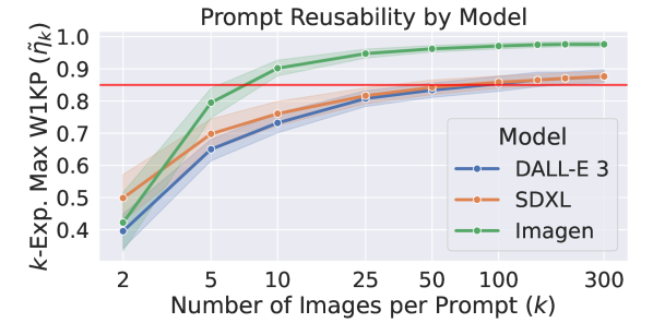
Figure 5: $k$-expected maximum ($\tilde{\eta}_{k}$) for $k=2$ to $300$. Shaded regions denote 95% confidence intervals and the red line $\beta_{\text{high}}$.

As visualized in Figure 4 and plotted in Figure 5, our diffusion models vary in reusability. DALL-E 3 on average does not generate highly similar images ($\tilde{\eta}_{k}\geq\beta_{\text{high}})$ until $k\to 200$, with our visualization (top two rows in Figure 4, one prompt each) displaying much green- and magenta-shifting until the last column. On the other hand, Imagen tends to produce duplicate images for $k\to 50$. At 50 images, the two overlaid images are nearly indistinguishable from the true-color image; see the third column. Figure 5 corroborates these visual results, with the red line ($\beta_{\text{high}}$) intersecting Imagen’s green line between 5–10 and DALL-E 3’s blue line at 50–100. It also suggests that SDXL resembles DALL-E 3 in prompt reusability; see the overlap between the two. We conclude that diffusion models differ in prompt reusability, possibly due to different decoder architectures. For example, DALL-E 3 and SDXL share the same U-Net architecture, whereas Imagen’s is sparsified Saharia et al. (2022).

4.2 Exploratory Factor Analysis

Our next two analyses relate various linguistic features of prompts such as syntactic complexity to perceptual variability. First, to understand the salient structure of these linguistic features, we conduct a factor analysis over DiffusionDB.

Setup. Our analysis emulates previous work in interpreting linguistic features for speech Fraser et al. (2016). We extracted 56 features for each of the 1,000 random prompts:

• Syntactic complexity: 24 scalar features related to syntax comprehension, such as clauses per T-unit and mean T-unit length, extracted using L2SCA Lu (2010). We also added Yngve depth, a measure of embeddedness Yngve (1960). Our motivation was that sentences with more qualifiers and nominals may be more visually precise.

• Keywords: 20 boolean features indicating the presence of the top-20 keywords. We had noticed that most prompts contained trailing keyword qualifiers after a noun phrase, e.g., “cat beside road, 4k” (see Appendix C for more); thus, we extracted the top 20 as features.

• Word order: 3 boolean features denoting the presence of the PTB Marcinkiewicz (1994) part-of-speech patterns “NN VB,” “NN VB RB,” and “JJ NN” in the prompt. Our purpose was to assess the effects of adjectives and verbs on nouns.

• Psycholinguistics: 4 features in mean concreteness judgements Brysbaert et al. (2014), richness (Honore’s statistic and whether a word was in a 100k-word dictionary), and word frequency Brysbaert and New (2009).

• Semantic relations: 3 scalars for the mean number of hyponyms, hypernyms, and word senses, from WordNet Miller (1995) enhanced with word sense clustering Snow et al. (2007). Intuitively, words with many synonyms (e.g., “saw”) or hyponyms (e.g., “animal”) may have more visual representations.

• Embedding norm: 2 scalars for the mean square GloVe norm Pennington et al. (2014) and CLIP embedding norm Radford et al. (2021). Word embedding norms were found to encode information gain Oyama et al. (2023), which may affect perceptual variability through specificity.

We generated 20 images per prompt for SDXL, Imagen, and DALL-E 3 and used Stanford CoreNLP Manning et al. (2014) as our parser (additional details in Appendix D.1).

#	Name	Fac. 1	Fac. 2	Fac. 3	Fac. 4	$\rho$	$\mu$
Factor 1: Style Keyword Presence; Mean $|\rho|=0.12$
1	Keyword: cgsociety	0.80				0.09	0.05
2	Keyword: 8k	0.75		-0.10		0.12	0.17
3	Keyword: detailed	0.75				0.14	0.05
4	Keyword: artgerm	0.66				0.15	0.06
5	Keyword: cinematic	0.59				0.11	0.04
6	Keyword: digital art	0.43				0.10	0.04
Factor 2: Syntactic Complexity; Mean $|\rho|=0.09$
7	Clauses per T-unit (T)		1.08	-0.13	-0.13	0.07	0.69
8	Clauses per sentence		0.92		-0.13	0.05	0.69
9	Number of T-units		0.63	-0.37	0.20	0.07	0.92
10	Verb phrases/T	-0.11	0.47			0.05	0.50
11	Complex nominals/T	-0.12	0.46	0.46	0.12	0.19	2.16
Factor 3: Linguistic Unit Length; Mean $|\rho|=0.19$
12	Mean T-unit length		0.49	0.60	0.17	0.18	16.7
13	Mean clause length		0.45	0.53	0.19	0.18	15.9
14	Mean sentence length			0.51	0.45	0.27	21.4
15	Coordinate phrases/T	0.15	0.20	0.27		0.13	0.33
Factor 4: Semantic Richness; Mean $|\rho|=0.17$
16	Number of words		0.12	0.11	0.75	0.30	24.6
17	CLIP embedding norm			0.17	-0.61	-0.31	151
18	ADJ NOUN				0.55	0.21	0.82
19	Percentage of keywords	0.20	0.11		0.55	0.20	48.8
20	Mean concreteness				0.47	0.25	2.30
21	Mean # of word senses	-0.11			0.43	-0.18	2.58
22	Honore’s statistic				-0.38	-0.09	7.36
23	Not in dictionary				0.29	0.09	0.91
24	Keyword: elegant				0.21	0.04	0.04
25	Keyword: fantasy				0.15	0.05	0.04

Table 2: Linguistic features grouped by interpreted factors, with high loadings ($\geq$0.3) in bold and low loadings ($<$0.1) removed. All Spearman’s $\rho$ are statistically significant ($p<0.05$); insignificant features omitted.

Results. We present our results in Table 2. Following standard practice Fraser et al. (2016), we use an oblique promax rotation to enable interfactor correlation. Four factors capture sufficient variance according to Kaiser’s criterion Kaiser (1958). For each feature, we report its correlation (Spearman’s $\rho$) with the per-prompt perceptual similarity ($\tilde{\eta}_{\text{mean}}$) and compute the mean feature score $\mu$.

As is conventional, we manually explain the four factors (F1–F4). For F1, “8k,” “detailed,” “cinematic,” and “digital art” describe the art style, “cgsociety” pertains to computer graphics, and “artgerm” is an artist with a specific style; hence, we call it “style keyword presence.” F2’s features are classic measures of syntactic complexity Lu (2010) and thus labeled as such. In F3, mean length of clauses, sentences, and T-units quantify various lengths, so we name it “linguistic unit length.” Lastly, F4 primarily depicts semantic richness, with concreteness, CLIP embedding norm (related to information gain), number of word senses, and ADJ NOUN roughly characterizing visual (non)ambiguity and Honore’s statistic, the number of words, and “not in dictionary” portraying lexical richness.

Our feature correlations with W1KP agree with intuition. Having higher concreteness (e.g., house vs. dignity) and fewer word senses (saw vs. tomato) increases similarity (rows 20, 21), likely since abstract and polysemous words have more visual interpretations. Complex nominals (row 11), adjectival modifiers (row 18), and keywords (F1) limit variability through qualification. Semantic richness has the strongest correlated features, with half having $|\rho|>0.2$. CLIP norm is the most predictive of variability ($\rho=-0.31$), possibly because text embeddings from vision-language models are used to initialize image generation (Sec. 2.1). Larger norms may yield more chaotic decoding trajectories in the iterative solver, increasing variability. Factor-wise, linguistic unit length has the highest mean $|\rho|$ of $0.19$, where sentence length is the third most predictive feature ($\rho=0.27$). Longer prompts presumably provide more visual information. We conclude that many features in the linguistic space are predictive of variability in the visual space, especially CLIP norm, length, and concreteness.

4.3 Confirmatory Lexical Analysis

The last section studies how prompts relate to variability in the DiffusionDB corpus. While it benefits from realism, some experimental control is lost. Thus, to supplement the previous study, this section uses single-word synthetic prompts, sampled and adjusted for word frequency in a clean-room manner. We examine the effects of concreteness, CLIP norm, and polysemy—three of the strongest features from Sec. 4.2.

Setup. For our prompts, we sampled 500 words from the 10k most common words in the Google Trillion Word Corpus Brants and Franz (2006). We noted each word’s concreteness rating ($x_{\text{conc}})$, number of word senses ($x_{\text{sens}}$), CLIP embedding norm ($x_{\text{clip}}$), and frequency rank ($x_{\text{freq}}$) as our explanatory variables, mirroring the setup of Section 4.2. Words without concreteness ratings were resampled. We then generated 20 images for each prompt with SDXL, Imagen, and DALL-E 3 and measured perceptual variability using $\tilde{\eta}_{\text{mean}}$. For our analysis, we fit a linear mixed model with $x_{\text{conc}}$, $x_{\text{sens}}$, $x_{\text{clip}}$, and $x_{\text{freq}}$ as the fixed effects, an intercept for each diffusion model as the random effect, and $\tilde{\eta}_{\text{mean}}$ as the response variable. Our purpose is to test whether concreteness, polysemy, CLIP norm, and word frequency independently influence perceptual variability for each model.

Results. Our linear mixed model reveals statistically significant relationships ($p<0.01$) between $\tilde{\eta}_{\text{mean}}$ and all the predictors, whose coefficients are $2.4\times 10^{-3}$, $4.7\times 10^{-4}$, $-7.8\times 10^{-5}$, and $-7.2\times 10^{-2}$ for $x_{\text{sens}}$, $x_{\text{clip}}$, $x_{\text{freq}}$, and $x_{\text{conc}}$, respectively. In other words, polysemy, CLIP norm, word frequency, and concreteness are significant independent factors for perceptual variability, where polysemy and CLIP norm are positively correlated, while frequency and concreteness negatively so. In Figure 6, our feature-wise plots further illustrate each individual fixed effect. The correlation scores are consistent in direction across the diffusion models, with similar signs in Spearman’s $\rho$ for each feature. They also differ by an additive shift, affirming our random-intercepts mixed model.

Figure 7 presents prompts of varying concreteness and senses. “Cowboy,” a concrete prompt, is less variable than “concept,” an abstract one, since a cowboy is tangible. “Tomato,” a monosemous word, has less variability than “saw,” a polysemous word, because it has a narrow visual representation. In summary, our exploratory findings on concreteness, CLIP norm, and polysemy from Section 4.2 hold in the clean-room single-word prompt setting.

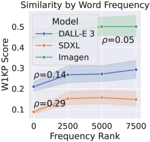
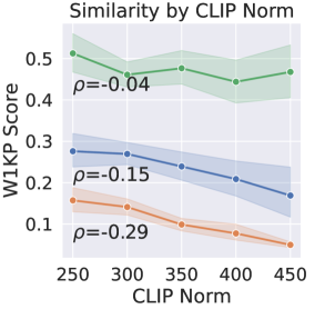
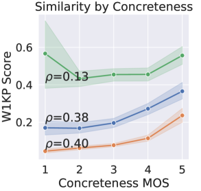
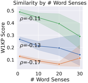
Figure 6: A plot of $\tilde{\eta}_{\text{mean}}$ against frequency, CLIP norm, concreteness, and word senses for single-word prompts. Shaded regions are 95% confidence intervals.

Figure 7: Four single-word Imagen prompts with varying concreteness (“cowboy” vs. “concept”) and number of word senses (“tomato” vs. “saw”).

5 Related Work and Future Directions

A related line of work examines boosting image variability in diffusion models Zameshina et al. (2023); Sadat et al. (2024); Gu et al. (2024). Complementary to their work, our paper analyzes the precise linguistic features contributing to variability. One future direction could be to incorporate these features into the optimization of variability.

Previous work has analyzed diffusion models using using a mixture of computational linguistics and vision techniques. Tang et al. (2023) conducted an attribution analysis over Stable Diffusion and discovered entanglement, to which Rassin et al. (2024) proposed to fix using attention alignment. Separately, Toker et al. (2024) studied the layer-intermediate representations of diffusion, showing that rare concepts require more computation. A further extension could be to study linguistic features responsible for increased computation, as our paper also relates word rarity to variability.

Finally, research has previously scrutinized the (lack of) variability in older architectures such as VAEs Razavi et al. (2019) and generative adversarial networks, e.g., mode collapse. In this paper, we extend this analysis to modern diffusion models while taking a visuolinguistic perspective.

6 Conclusions

In conclusion, we examined the connection between visual variability and prompt language for black-box diffusion models. We proposed a framework for quantifying and calibrating visual variability, applying it to study prompt reusability and linguistic feature salience. After validating it quantitatively, we found that length, embedding norm, and concreteness influence variability the most.

Limitations

One limitation of our work is that while we analyzed the inference-time behavior of various diffusion models, we did not trace the training-time cause of perceptual variability due to the scope of our study. Doing so would require the training of multiple diffusion models while varying the training sets, which is beyond our budget.

Another limitation is that we have not meticulously characterized the precise distribution of perceptual variability relative to various levels of linguistic features, with our analyses constrained to averages due to the moderate sample size. For instance, does Imagen yield a higher maximum variability for certain levels of concreteness, even if on average it is lower? Are there subgroups within each feature that better explain variances in perceptual variability? Such questions require a larger sample size to answer.

To limit the scope of the paper, we also consciously restricted our examination to random seeds and dispensed with comprehensively assessing other factors possibly influencing perceptual variability, such as classifier-free guidance Ho and Salimans (2021). We briefly vary the guidance scale in Appendix D.2 to confirm that SDXL is always more diverse than Imagen regardless of guidance; nevertheless, a full study with additional factors other than linguistic features and random seeds could yield further insights.

Finally, it should be noted that our work intentionally disregards the relationship between quality and variability, although the two can be conflated. For example, does increased variability reduce image quality? Is Imagen a better option than, say, SDXL due to its higher quality, even if it generates less diverse imagery? Thus, text-to-image models should not be chosen based on the findings of our study alone. Rather, our work supplements image quality metrics in model selection.

Appendix A Detailed Experimental Settings

A.1 Computational Environment

Our primary software toolkits included HuggingFace Diffusers 0.25.0, Transformers 4.40.1, PyTorch 2.1.2, DreamSim 0.1.3, and CUDA 12.2. We ran all experiments on a machine with four Nvidia A6000 GPUs and an AMD Epyc Milan CPU.

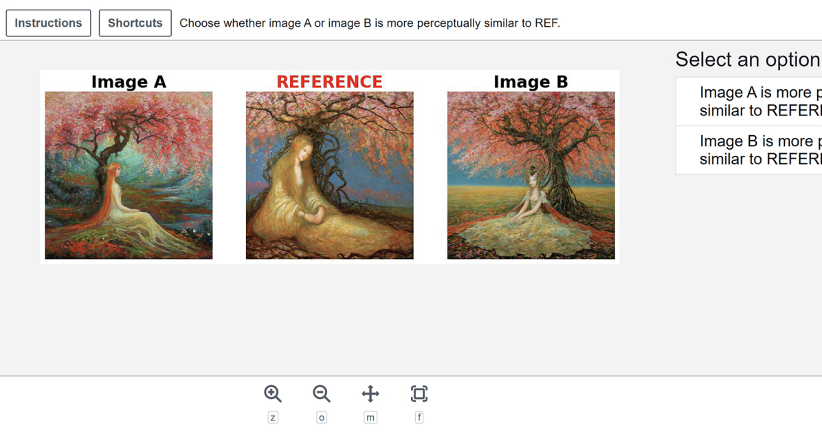
Figure 8: Interface for collecting 2AFC judgements.

A.2 Diffusion Model Details

SDXL. We downloaded stabilityai/stable- diffusion-xl-base-1.0 from HuggingFace zoo. We used the default guidance scale of 7.5 and 30 inference steps without the additional refiner module. Each 1024x1024 SDXL image took 4–5 seconds to generate per card, resulting in a throughput of roughly 50–60 images per minute.

Imagen. We selected the imagegeneration@006 model, the latest version as of April 2024, and generated four square images per call while varying the random seed. This matched our SDXL throughput of 50–60 images per minute. Each image was 1536x1536 in resolution.

DALL-E 3. For DALL-E 3, we used the default parameters of “hd” resolution (1024x1024) and “vivid” style. To mitigate prompt editing, we followed the official documentation and prepended “I NEED to test how the tool works with extremely simple prompts. DO NOT add any detail, just use it AS-IS: ” to the prompt. The generation speed of DALL-E 3 was considerably slower than Imagen and SDXL at approximately 10 images per minute.

A.3 Annotation Apparatuses

W1KP quality. We present the annotation user interface for collecting 2AFC judgements in Figure 8. For our attention checks, we showed each worker at least one triplet with either image A or B exactly matching the reference. If the correct answer was not chosen, we rejected all their labels and blocked them. This resulted in a pass rate of around 90%. For higher quality, we required our workers to be “Masters” for participation eligibility.

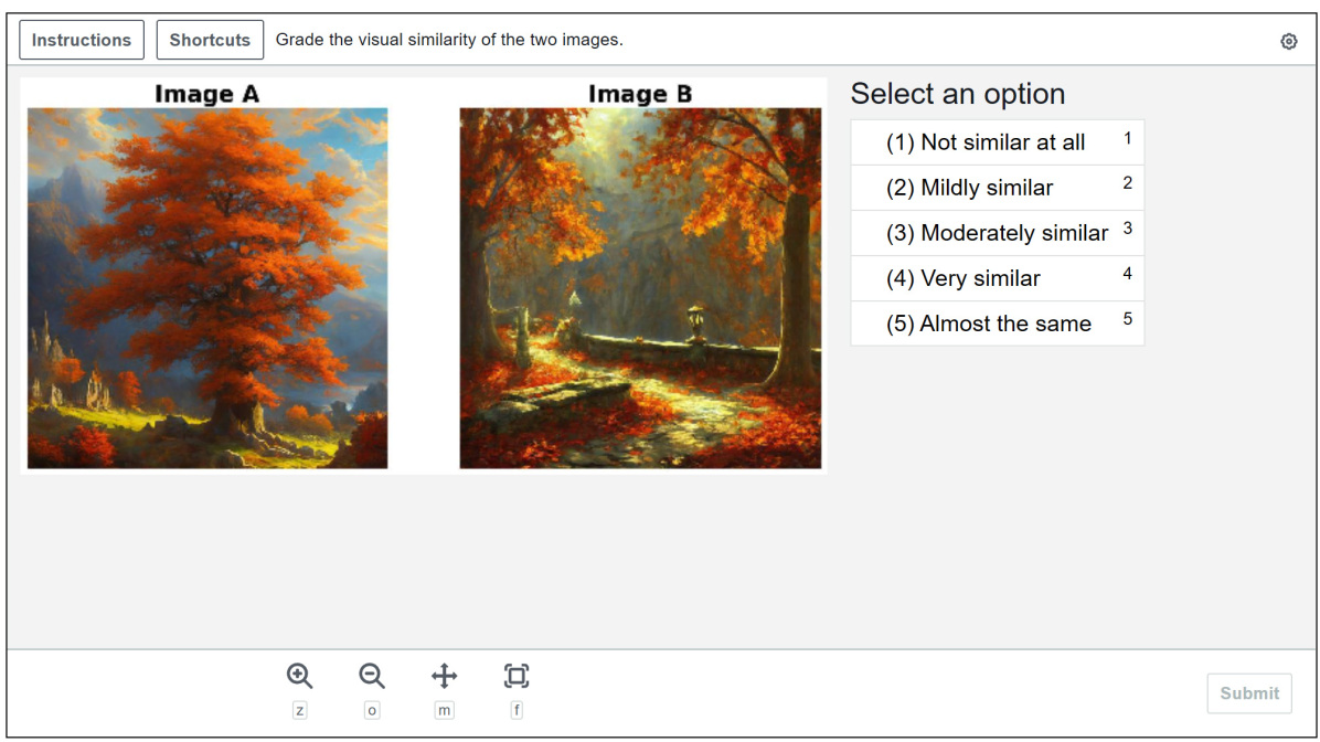
Figure 9: Interface for collecting graded judgements.

W1KP metric interpretation. We present our annotation interface for gathering graded similarity judgements in Figure 9. For the attention checks, we showed each annotator at least one pair of images that were the exact same. If they did not choose “almost the same,” we discarded all their judgements, resulting in an acceptance rate of 95%.

Appendix B Detailed Proofs

Proposition 2.1. If $X$ is a continuous random variable, $F(X)$ is standard uniform $U[0,1]$.

Proof.

Let $X$ be a continuous r.v. If $X$ is $U[0,1]$, then its CDF $\mathbb{P}(X\leq x)=x$. Since $\mathbb{P}(F(X)\leq x)=\mathbb{P}(X\leq F^{-1}(x))=F(F^{-1}(x))=x$, then $F(X)$ is $U[0,1]$, completing our proof. ∎

Proposition 2.2. If $d$ is the squared Euclidean distance and $h$ the pairwise mean kernel, $U_{d,h}$ is proportional to the trace of the covariance matrix of $f(I_{1}),\dots,f(I_{n})$, i.e., the total variance.

Proof.

Consider the pairwise sum squared Euclidean distance $\sum_{i\neq j}||f(I_{i})-f(I_{j})||^{2}_{2}$, which expands into

$$\sum_{i\neq j}f(I_{i})^{\intercal}f(I_{i})-2f(I_{i})^{\intercal}f(I_{j})+f(I_{j})^{\intercal}f(I_{j}).$$ (4)

The first and third self-product terms expands as

$$(n-1)\sum_{i=1}^{n}f(I_{i})^{\intercal}f(I_{i})$$ (5)

and

$$(n-1)\sum_{j=1}^{n}f(I_{j})^{\intercal}f(I_{j}),$$ (6)

and the middle term

$$\sum_{i,j}f(I_{i})^{\intercal}f(I_{j})-\sum_{i=1}^{n}f(I_{i})^{\intercal}f(I_{i}).$$ (7)

After algebraic manipulation, we arrive at

$$(n-1)\left(\frac{1}{n}\sum_{i=1}^{n}f(I_{i})^{\intercal}f(I_{i})-\frac{1}{n^{2}}\sum_{i,j}f(I_{i})^{\intercal}f(I_{j})\right).$$ (8)

We are ready to relate this quantity to the trace of the covariance matrix, given by

$$\text{tr}(\Lambda)=\frac{1}{n}\sum_{i=1}^{n}||f(I_{i})-\frac{1}{n}\sum_{j=1}^{n}f(I_{j})||_{2}^{2},$$ (9)

which simplifies as

$$\frac{1}{n}\left(\sum_{i=1}^{n}f(I_{i})^{\intercal}f(I_{i})-\frac{1}{n}\sum_{i,j}f(I_{i})^{\intercal}f(I_{j})\right).$$ (10)

Multiplying by $(n-1)$, we arrive at the sum of the pairwise squared Euclidean distance. Dividing by $n(n-1)$ yields the mean pairwise squared distance, and our proof is finished. ∎

Appendix C DiffusionDB Statistics

We now characterize the prompts and keywords in DiffusionDB. To extract trailing keywords, we split prompts into a main part and its keywords part by applying these steps:

1. Tokenize the prompt by commas, e.g., “cat walking, 4k” becomes “cat walking” and “4k.”

2. If any “token” after the first is shorter than four words, everything after that token is considered a keyword.

3. The first “token” is always the main prompt.

A preliminary analysis showed that this was more than 95% accurate in identifying keywords. We present ten examples below:

1. “ashtray in the messy desk of the detective, smoke and dark, digital art”

2. “onion very sad crying big tears cartoon, 3d render”

3. “the lost city of Atlantis, 4K, hyper detailed”

4. “a galleon ship by Darek Zabrocki”

5. “hill overlooking a viking city, fantasy, forested, large trees, top down perspective, […]”

6. “photo of an awesome sunny day environment concept art on a cliff, architecture by daniel libeskind with village, residential area, mixed development, highrise made up staircases, […]”

7. “giant oversized battle hedgehog with army pilot uniform and hedgehog babies ,in deep forest hungle , full body , Cinematic focus, Polaroid photo, vintage , neutral dull colors, soft lights, […]”

8. “pizza the hut, akira, gorillaz, poster, high quality”

9. “tengu spotted in atlanta”

10. “underground cinema, realistic architecture, colorfull lights, octane render, 4k, 8k”

Appendix D Visuolinguistic Analysis Details

D.1 Linguistic Feature Extraction

For word sense clustering, we used the “WN 2.1 -19370 synsets” resource from https://ai.stanford.edu/~rion/swn/, previously published in Snow et al. (2007). Unless otherwise stated, all our CLIP models were initialized from the openai/clip-vit-large-patch14-336 checkpoint from HuggingFace, released by OpenAI. Our GloVe embeddings were the 300-dimensional embeddings trained on 840B tokens of web text.

D.2 Effects of Classifier-Free Guidance

We briefly confirmed that increasing classifier-free guidance did not worsen the perceptual variability of SDXL below that of Imagen. Imagen and DALL-E 3 do not expose classifier-free guidance as an input parameter, hence limiting us to SDXL. We increased the classifier-free guidance from 5.0 to 30, much higher than the normal range of 5.0–7.5, and regenerated the images in Section 4.1. We arrived at a mean W1KP score of 0.53 for SDXL, which was below Imagen’s score of 0.62, e.g., SDXL still had greater variability.

Appendix E Dimensionality-Reducing Visualization

   

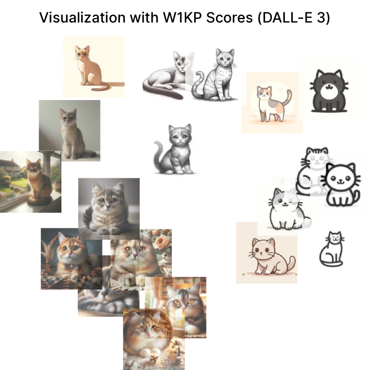
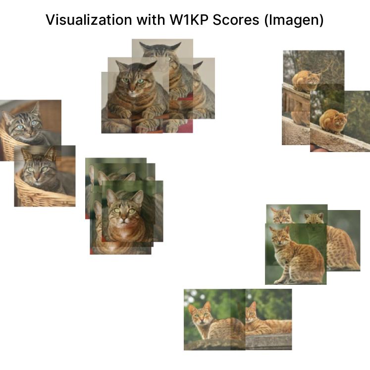
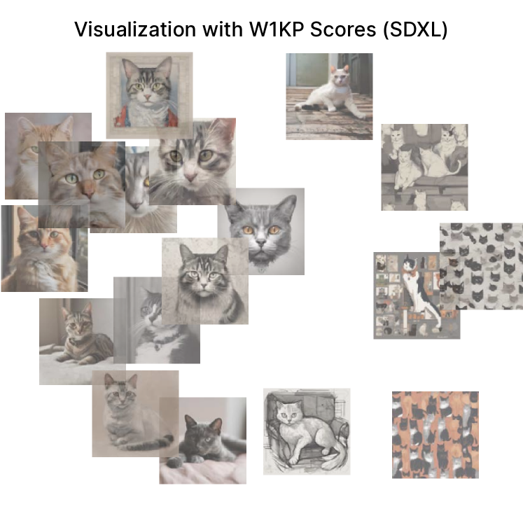
Figure 10: Twenty generated images for the prompt “cat,” clustered using multidimensional scaling on DreamSim${}_{\ell_{2}}$. Imagen produces six distinct clusters.

   

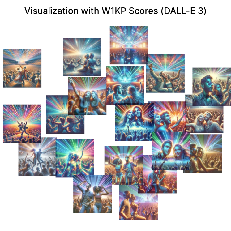
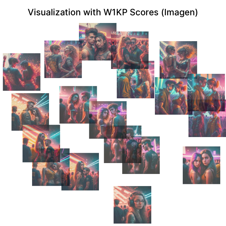
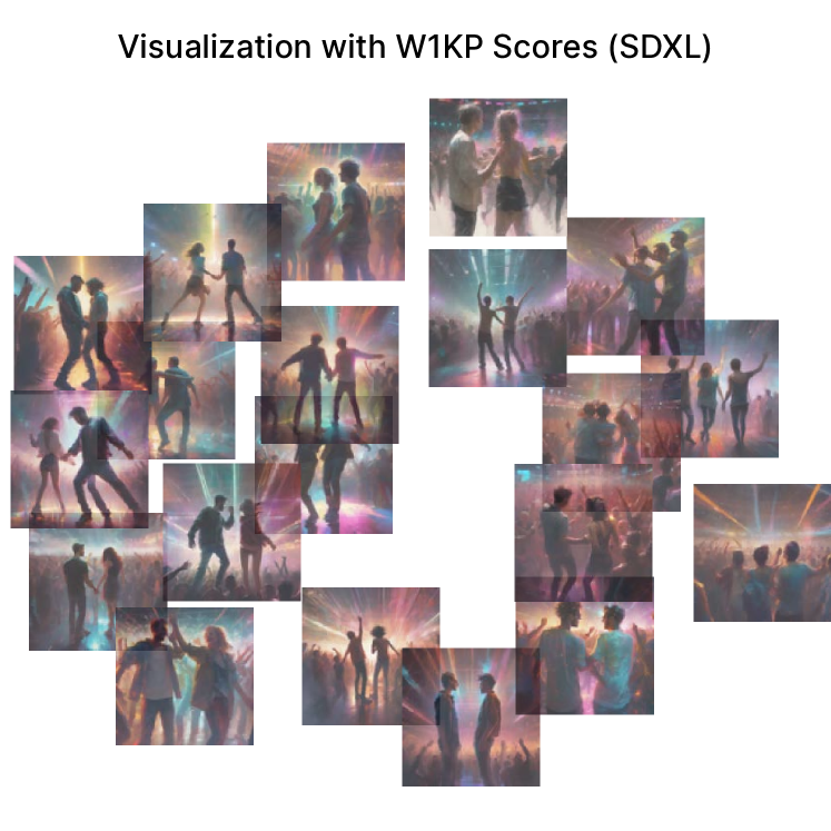
Figure 11: Generated images for a longer prompt.

References

- Acuna et al. (2015) Daniel E. Acuna, Max Berniker, Hugo L. Fernandes, and Konrad P. Kording. 2015. Using psychophysics to ask if the brain samples or maximizes. Journal of vision.
- Betker et al. (2023) James Betker, Gabriel Goh, Li Jing, Tim Brooks, Jianfeng Wang, Linjie Li, Long Ouyang, Juntang Zhuang, Joyce Lee, Yufei Guo, et al. 2023. Improving image generation with better captions. OpenAI Blog.
- Brants and Franz (2006) Thorsten Brants and Alex Franz. 2006. Web 1T 5-gram version 1. Linguistic Data Consortium.
- Brysbaert and New (2009) Marc Brysbaert and Boris New. 2009. Moving beyond kučera and francis: A critical evaluation of current word frequency norms and the introduction of a new and improved word frequency measure for american english. Behavior research methods.
- Brysbaert et al. (2014) Marc Brysbaert, Amy Beth Warriner, and Victor Kuperman. 2014. Concreteness ratings for 40 thousand generally known English word lemmas. Behavior research methods.
- Ding et al. (2020) Keyan Ding, Kede Ma, Shiqi Wang, and Eero P. Simoncelli. 2020. Image quality assessment: Unifying structure and texture similarity. IEEE transactions on pattern analysis and machine intelligence.
- Dosovitskiy et al. (2021) Alexey Dosovitskiy, Lucas Beyer, Alexander Kolesnikov, Dirk Weissenborn, Xiaohua Zhai, Thomas Unterthiner, et al. 2021. An image is worth 16x16 words: Transformers for image recognition at scale. In ICLR.
- Fraser et al. (2016) Kathleen C. Fraser, Jed A. Meltzer, and Frank Rudzicz. 2016. Linguistic features identify Alzheimer’s disease in narrative speech. Journal of Alzheimer’s disease.
- Fu et al. (2024) Stephanie Fu, Netanel Tamir, Shobhita Sundaram, Lucy Chai, Richard Zhang, Tali Dekel, and Phillip Isola. 2024. DreamSim: Learning new dimensions of human visual similarity using synthetic data. NeurIPS.
- Ghildyal and Liu (2022) Abhijay Ghildyal and Feng Liu. 2022. Shift-tolerant perceptual similarity metric. In ECCV.
- Gu et al. (2024) Jiatao Gu, Ying Shen, Shuangfei Zhai, Yizhe Zhang, Navdeep Jaitly, and Joshua M. Susskind. 2024. Kaleido diffusion: Improving conditional diffusion models with autoregressive latent modeling. arXiv:2405.21048.
- Hauser and Schwarz (2016) David J. Hauser and Norbert Schwarz. 2016. Attentive turkers: MTurk participants perform better on online attention checks than do subject pool participants. Behavior research methods.
- Ho and Salimans (2021) Jonathan Ho and Tim Salimans. 2021. Classifier-free diffusion guidance. In NeurIPS 2021 Workshop on Deep Generative Models and Downstream Applications.
- Hoeffding (1948) Wassily Hoeffding. 1948. A class of statistics with asymptotically normal distribution. The Annals of Mathematical Statistics.
- Kaiser (1958) Henry F. Kaiser. 1958. The varimax criterion for analytic rotation in factor analysis. Psychometrika.
- Li et al. (2022) Hongwei Bran Li, Chinmay Prabhakar, Suprosanna Shit, Johannes Paetzold, Tamaz Amiranashvili, Jianguo Zhang, Daniel Rueckert, et al. 2022. A domain-specific perceptual metric via contrastive self-supervised representation: Applications on natural and medical images. arXiv:2212.01577.
- Li (2012) Hongzhe Li. 2012. U-statistics in genetic association studies. Human genetics.
- Lu (2010) Xiaofei Lu. 2010. Automatic analysis of syntactic complexity in second language writing. International journal of corpus linguistics.
- Manning et al. (2014) Christopher D. Manning, Mihai Surdeanu, John Bauer, Jenny Rose Finkel, Steven Bethard, and David McClosky. 2014. The Stanford CoreNLP natural language processing toolkit. In ACL: System Demonstrations.
- Marcinkiewicz (1994) Mary Ann Marcinkiewicz. 1994. Building a large annotated corpus of English: The Penn treebank. Using Large Corpora.
- Miller (1995) George A. Miller. 1995. WordNet: a lexical database for English. Communications of the ACM.
- Oyama et al. (2023) Momose Oyama, Sho Yokoi, and Hidetoshi Shimodaira. 2023. Norm of word embedding encodes information gain. In EMNLP.
- Pennington et al. (2014) Jeffrey Pennington, Richard Socher, and Christopher D. Manning. 2014. GloVe: Global vectors for word representation. In Empirical Methods in Natural Language Processing.
- Pizzi et al. (2022) Ed Pizzi, Sreya Dutta Roy, Sugosh Nagavara Ravindra, Priya Goyal, and Matthijs Douze. 2022. A self-supervised descriptor for image copy detection. In CVPR.
- Podell et al. (2024) Dustin Podell, Zion English, Kyle Lacey, Andreas Blattmann, Tim Dockhorn, Jonas Müller, Joe Penna, and Robin Rombach. 2024. SDXL: Improving latent diffusion models for high-resolution image synthesis. In ICLR.
- Radford et al. (2021) Alec Radford, Jong Wook Kim, Chris Hallacy, Aditya Ramesh, Gabriel Goh, Sandhini Agarwal, Girish Sastry, Amanda Askell, Pamela Mishkin, Jack Clark, Gretchen Krueger, and Ilya Sutskever. 2021. Learning transferable visual models from natural language supervision. In ICML.
- Raffel et al. (2020) Colin Raffel, Noam Shazeer, Adam Roberts, Katherine Lee, Sharan Narang, Michael Matena, Yanqi Zhou, Wei Li, and Peter J. Liu. 2020. Exploring the limits of transfer learning with a unified text-to-text transformer. The Journal of Machine Learning Research.
- Rassin et al. (2024) Royi Rassin, Eran Hirsch, Daniel Glickman, Shauli Ravfogel, Yoav Goldberg, and Gal Chechik. 2024. Linguistic binding in diffusion models: Enhancing attribute correspondence through attention map alignment. NeurIPS.
- Razavi et al. (2019) Ali Razavi, Aaron Van den Oord, and Oriol Vinyals. 2019. Generating diverse high-fidelity images with VQ-VAE-2. NeurIPS.
- Rombach et al. (2022) Robin Rombach, Andreas Blattmann, Dominik Lorenz, Patrick Esser, and Björn Ommer. 2022. High-resolution image synthesis with latent diffusion models. In CVPR.
- Ronneberger et al. (2015) Olaf Ronneberger, Philipp Fischer, and Thomas Brox. 2015. U-Net: Convolutional networks for biomedical image segmentation. In International Conference on Medical Image Computing and Computer-Assisted Intervention.
- Sadat et al. (2024) Seyedmorteza Sadat, Jakob Buhmann, Derek Bradley, Otmar Hilliges, and Romann M. Weber. 2024. CADS: Unleashing the diversity of diffusion models through condition-annealed sampling. In ICLR.
- Saharia et al. (2022) Chitwan Saharia, William Chan, Saurabh Saxena, Lala Li, Jay Whang, Emily Denton, et al. 2022. Photorealistic text-to-image diffusion models with deep language understanding. arXiv:2205.11487.
- Schuhmann et al. (2022) Christoph Schuhmann, Romain Beaumont, Cade W. Gordon, Ross Wightman, Theo Coombes, et al. 2022. LAION-5B: An open large-scale dataset for training next generation image-text models.
- Simonyan and Zisserman (2015) Karen Simonyan and Andrew Zisserman. 2015. Very deep convolutional networks for large-scale image recognition. In ICLR.
- Snow et al. (2007) Rion Snow, Sushant Prakash, Dan Jurafsky, and Andrew Y. Ng. 2007. Learning to merge word senses. In EMNLP-IJCNLP.
- Song et al. (2021) Yang Song, Jascha Sohl-Dickstein, Diederik P. Kingma, Abhishek Kumar, Stefano Ermon, and Ben Poole. 2021. Score-based generative modeling through stochastic differential equations. In ICLR.
- Tang et al. (2023) Raphael Tang, Linqing Liu, Akshat Pandey, Zhiying Jiang, Gefei Yang, Karun Kumar, Pontus Stenetorp, Jimmy Lin, and Ferhan Türe. 2023. What the DAAM: Interpreting stable diffusion using cross attention. In ACL.
- Toker et al. (2024) Michael Toker, Hadas Orgad, Mor Ventura, Dana Arad, and Yonatan Belinkov. 2024. Diffusion lens: Interpreting text encoders in text-to-image pipelines. In ACL.
- Wang et al. (2004) Zhou Wang, Alan C. Bovik, Hamid R Sheikh, and Eero P. Simoncelli. 2004. Image quality assessment: from error visibility to structural similarity. IEEE transactions on image processing.
- Wang et al. (2023) Zijie J. Wang, Evan Montoya, David Munechika, Haoyang Yang, Benjamin Hoover, and Duen Horng Chau. 2023. DiffusionDB: A large-scale prompt gallery dataset for text-to-image generative models. In ACL.
- Yngve (1960) Victor H. Yngve. 1960. A model and an hypothesis for language structure. Proceedings of the American philosophical society.
- Zameshina et al. (2023) Mariia Zameshina, Olivier Teytaud, and Laurent Najman. 2023. Diverse diffusion: Enhancing image diversity in text-to-image generation. arXiv:2310.12583.
- Zhang et al. (2018) Richard Zhang, Phillip Isola, Alexei A. Efros, Eli Shechtman, and Oliver Wang. 2018. The unreasonable effectiveness of deep features as a perceptual metric. In CVPR.