Nyström Kernel Stein Discrepancy

Florian Kalinke1,  Zoltán Szabó2,  Bharath K. Sriperumbudur3
1Karlsruhe Institute of Technology, Karlsruhe, Germany
2London School of Economics, London, UK
3The Pennsylvania State University, University Park, PA 16802, USA
florian.kalinke@kit.edu      z.szabo@lse.ac.uk      bks18@psu.edu
Abstract

Kernel methods underpin many of the most successful approaches in data science and statistics, and they allow representing probability measures as elements of a reproducing kernel Hilbert space without loss of information. Recently, the kernel Stein discrepancy (KSD), which combines Stein’s method with kernel techniques, gained considerable attention. Through the Stein operator, KSD allows the construction of powerful goodness-of-fit tests where it is sufficient to know the target distribution up to a multiplicative constant. However, the typical U- and V-statistic-based KSD estimators suffer from a quadratic runtime complexity, which hinders their application in large-scale settings. In this work, we propose a Nyström-based KSD acceleration—with runtime $\mathcal{O}\!\left(mn+m^{3}\right)$ for $n$ samples and $m\ll n$ Nyström points—, show its $\sqrt{n}$-consistency under the null with a classical sub-Gaussian assumption, and demonstrate its applicability for goodness-of-fit testing on a suite of benchmarks.

1 Introduction

The kernel mean embedding, which involves mapping probabilities into a reproducing kernel Hilbert spaces (RKHS; Aronszajn 1950) has found far-reaching applications in the last $20$ years. For example, it allows to measure the discrepancy between probability distributions through maximum mean discrepancy (MMD; Smola et al. 2007, Gretton et al. 2012), defined as the distance between the corresponding mean embeddings, which underpins powerful two-sample tests. MMD is also known as energy distance [Székely and Rizzo, 2004, 2005, Baringhaus and Franz, 2004] in the statistics literature; see Sejdinovic et al. [2013] for the equivalence. We refer to [Muandet et al., 2017] for a recent overview of kernel mean embeddings.

In addition to two-sample tests, testing for goodness-of-fit (GoF; Ingster and Suslina 2003, Lehmann and Romano 2021) is also of central importance in data science and statistics, which involves testing $H_{0}:\mathbb{Q}=\mathbb{P}$ vs. $H_{1}:\mathbb{Q}\neq\mathbb{P}$ based on samples from an unknown sampling distribution $\mathbb{Q}$ and a (fixed known) target distribution $\mathbb{P}$. Classical GoF tests, e.g., the Kolmogorov-Smirnov test [Kolmogorov, 1933, Smirnov, 1948], or the test for normality by Baringhaus and Henze [1988], usually require explicit knowledge of the target distribution. However, in practical applications, the target distribution is frequently only known up to a normalizing constant. Examples include validating the output of Markov Chain Monte Carlo (MCMC) samplers [Welling and Teh, 2011, Bardenet et al., 2014, Korattikara et al., 2014], or assessing deep generative models [Koller and Friedman, 2009, Salakhutdinov, 2015]. In all these examples, one desires a powerful test, even though the normalization constant might be difficult to obtain.

A recent approach to tackle GoF testing involves applying a Stein operator [Stein, 1972, Chen, 2021, Anastasiou et al., 2023] to functions in an RKHS and using them as test functions to measure the discrepancy between distributions, referred to as kernel Stein discrepancies (KSD; Chwialkowski et al. 2016, Liu et al. 2016). An empirical estimator of KSD can be used as a test statistic to address the GoF problem. In particular, the Langevin Stein operator [Gorham and Mackey, 2015, Chwialkowski et al., 2016, Liu et al., 2016, Oates et al., 2017, Gorham and Mackey, 2017] in combination with the kernel mean embedding gives rise to a KSD on the Euclidean space $\mathbb{R}^{d}$, which we consider in this work. As a test statistic, KSD has many desirable properties. In particular, KSD requires only knowledge of the derivative of the score function of the target distribution — implying that KSD is agnostic to the normalization of the target and therefore does not require solving, either analytically or numerically, complex normalization integrals in Bayesian settings. This property has led to its widespread use, e.g., for assessing and improving sample quality [Gorham and Mackey, 2015, Chen et al., 2018, 2019, Futami et al., 2019, Gorham et al., 2020], validating MCMC methods [Coullon et al., 2023], comparing deep generative models [Lim et al., 2019], detecting out-of-distribution inputs [Nalisnick et al., 2019], assessing Bayesian seismic inversion [Izzatullah et al., 2020], modeling counterfactuals [Martinez-Taboada and Kennedy, 2023], and explaining predictions [Sarvmaili et al., 2024]. GoF testing with KSDs has been explored on Euclidean data [Liu et al., 2016, Chwialkowski et al., 2016], discrete data [Yang et al., 2018], point processes [Yang et al., 2019], time-to-event data [Fernandez et al., 2020], graph data [Xu and Reinert, 2021], sequential models [Baum et al., 2023], and functional data [Wynne et al., 2024]. The KSD statistic has also been extended to the conditional case [Jitkrittum et al., 2020].

Estimators for Langevin Stein operator-based KSD exist. But, the classical U-statistic- [Liu et al., 2016] and V-statistic-based [Chwialkowski et al., 2016] estimators have a runtime complexity that scales quadratically with the number of samples of the sampling distribution, which limits their deployment to large-scale settings. To address this bottleneck, Chwialkowski et al. [2016] introduced a linear-time statistic that suffers from low statistical power compared to its quadratic-time counterpart. Jitkrittum et al. [2017] proposed the finite set Stein discrepancy (FSSD), a linear-time approach that replaces the RKHS-norm by the $L_{2}$-norm approximated by sampling; the sampling can either be random (FSSD-rand) or optimized w.r.t. a power proxy (FSSD-opt). Another approach [Huggins and Mackey, 2018] is employing the random Fourier feature (RFF; Rahimi and Recht 2007) method to accelerate the KSD estimation. However, it is known [Chwialkowski et al., 2015, Proposition 1] that the resulting statistic fails to distinguish a large class of measures. Huggins and Mackey [2018] generalize the idea of replacing the RKHS-norm by going from $L_{2}$-norms to $L_{p}$ ones, to obtain feature Stein discrepancies. They present an efficient approximation, random feature Stein discrepancies (RFSD), which is a near-linear time estimator. However, successful deployment of the method depends on a good choice of parameters, which, while the authors provide guidelines, can be challenging to select and tune in practice.

Our work alleviates these severe bottlenecks. We employ the Nyström method [Williams and Seeger, 2001] to accelerate KSD estimation and show the $\sqrt{n}$-consistency of our proposed estimator under the null. The main technical challenge is that the Stein kernel (induced by the Langevin Stein operator and the original kernel) is typically unbounded while existing statistical Nyström analysis [Rudi et al., 2015, Chatalic et al., 2022, Sterge and Sriperumbudur, 2022, Kalinke and Szabó, 2023] usually considers bounded kernels. To tackle unbounded kernels, we select a classical sub-Gaussian assumption, which we impose on the feature map associated to the kernel, and show that existing methods of analysis can successfully be extended to handle this novel case. In this sense, our work, besides Della Vecchia et al. [2021], which requires a similar sub-Gaussian condition for analyzing empirical risk minimization on random subspaces, is a first step in analyzing the consistency of the unbounded case in the Nyström setting.

Our main contributions can be summarized as follows.

  1. 1.

    We introduce a Nyström-based acceleration of kernel Stein discrepancy. The proposed estimator runs in $\mathcal{O}\left(mn+m^{3}\right)$ time, with $n$ samples and $m\ll n$ Nyström points.

  2. 2.

    We prove the $\sqrt{n}$-consistency under the null of our estimator in a classical sub-Gaussian setting, which extends (in a non-trivial fashion) existing results for Nyström-based methods [Rudi et al., 2015, Chatalic et al., 2022, Sterge and Sriperumbudur, 2022, Kalinke and Szabó, 2023] focusing on bounded kernels.

  3. 3.

    We perform an extensive suite of experiments to demonstrate the applicability of the proposed method. Our proposed approach achieves competitive results throughout all experiments.

The paper is structured as follows. We introduce the notations used throughout the article (Section 2) followed by recalling the classical quadratic-time KSD estimators (Section 3). In Section 4.1, we detail our proposed Nyström-based estimator, alongside with its adaptation to a modified wild bootstrap goodness-of-fit test (Section 4.2), and our theoretical guarantees (Section 4.3). Experiments demonstrating the efficiency of our Nyström-KSD estimator are provided in Section 5. Proofs are deferred to the appendices.

2 Notations

In this section, we introduce our notations. Let $[N]:=\{1,\ldots,N\}$ for a positive integer $N$. For $a_{1},a_{2}\geq 0$, $a_{1}\lesssim a_{2}$ (resp. $a_{1}\gtrsim a_{2}$) means that $a_{1}\leq ca_{2}$ (resp. $a_{1}\geq c^{\prime}a_{2}$) for an absolute constant $c>0$ (resp. $c^{\prime}>0$), and we write $a_{1}\asymp a_{2}$ iff. $a_{1}\lesssim a_{2}$ and $a_{1}\gtrsim a_{2}$. We write $\mathds{1}_{(\cdot)}$ for the indicator function and $\left\{\left\{\cdot\right\}\right\}$ for a multiset. The $n$-dimensional vector of ones is denoted by $\bm{1}_{n}=\left(1,\ldots,1\right)^{\mkern-1.5mu\mathsf{T}}\in\mathbb{R}^{n}$ , that of $n$ zeros by $\bm{0}_{n}=\left(0,\ldots,0\right)^{\mkern-1.5mu\mathsf{T}}\in\mathbb{R}^{n}$. The identity matrix is $\mathbf{I}_{n}\in\mathbb{R}^{n\times n}$. For a matrix $\mathbf{A}\in\mathbb{R}^{d_{1}\times d_{2}}$, $\mathbf{A}^{-}\in\mathbb{R}^{d_{2}\times d_{1}}$ denotes its (Moore-Penrose) pseudo-inverse, and $\mathbf{A}^{\mkern-1.5mu\mathsf{T}}\in\mathbb{R}^{d_{2}\times d_{1}}$ stands for the transpose of $\mathbf{A}$. We write $\mathbf{A}^{-1}\in\mathbb{R}^{d\times d}$ for the inverse of a non-singular matrix $\mathbf{A}\in\mathbb{R}^{d\times d}$. For a differentiable function $f:\mathbb{R}^{d}\rightarrow\mathbb{R}$ , let $\nabla_{\mathbf{x}}f(\mathbf{x})=\left(\frac{\partial f(\mathbf{x})}{\partial x_{i}}\right)_{i=1}^{d}\in\mathbb{R}^{d}$.

Let $\left(\mathcal{X},\tau_{\mathcal{X}}\right)$ be a topological space and $\mathcal{B}\left(\tau_{\mathcal{X}}\right)$ the corresponding Borel $\sigma$-algebra. Probability measures in this article are meant w.r.t. the measurable space $\left(\mathcal{X},\mathcal{B}\left(\tau_{\mathcal{X}}\right)\right)$ and are written as $\mathcal{M}_{1}^{+}\left(\mathcal{X}\right)$; for instance, the set of Borel probability measures on $\mathbb{R}^{d}$ is $\mathcal{M}_{1}^{+}\left(\mathbb{R}^{d}\right)$. The $n$-fold product measure of $\mathbb{P}\in\mathcal{M}_{1}^{+}\left(\mathcal{X}\right)$ is denoted by $\mathbb{P}^{n}\in\mathcal{M}_{1}^{+}\left(\mathcal{X}^{n}\right)$. For a sequence of real-valued random variables $X_{n}$ and a sequence of positive $r_{n}$-s, $X_{n}=\mathcal{O}_{\mathbb{P}}(r_{n})$ means that $\frac{X_{n}}{r_{n}}$ is bounded in probability. The unit ball in a Hilbert space $\mathcal{H}$ is denoted by $B(\mathcal{H})=\left\{f\in\mathcal{H}\mid\left\|f\right\|_{\mathcal{H}}\leq 1\right\}$. The reproducing kernel Hilbert space with $k:\mathbb{R}^{d}\times\mathbb{R}^{d}\rightarrow\mathbb{R}$ as the reproducing kernel is denoted by $\mathcal{H}_{k}$. Throughout the paper, $k$ is assumed to be measurable and $\mathcal{H}_{k}$ to be separable; for instance, a continuous kernel $k:\mathbb{R}^{d}\times\mathbb{R}^{d}\to\mathbb{R}$ implies the latter property [Steinwart and Christmann, 2008, Lemma 4.33]. The canonical feature map $\phi_{k}:\mathbb{R}^{d}\to\mathcal{H}_{k}$ is defined as $\mathbf{x}\mapsto k(\cdot,\mathbf{x})$; with this feature map $k(\mathbf{x},\mathbf{y})=\left\langle{k(\cdot,\mathbf{x}),k(\cdot,\mathbf{y})}\right\rangle_{\mathcal{H}_{k}}=\left\langle{\phi_{k}(\mathbf{x}),\phi_{k}(\mathbf{y})}\right\rangle_{\mathcal{H}_{k}}$ for all $\mathbf{x},\mathbf{y}\in\mathbb{R}^{d}$. The Gram matrix associated with the observations $\left(\mathbf{x}_{i}\right)_{i=1}^{n}\in\left(\mathbb{R}^{d}\right)^{n}$ and kernel $k$ is $\mathbf{K}_{k,n,n}=\left[k(\mathbf{x}_{i},\mathbf{x}_{j})\right]_{i,j=1}^{n}\in\mathbb{R}^{n\times n}$. Given a closed linear subspace $U\subseteq\mathcal{H}_{k}$, the (orthogonal) projection of $h\in\mathcal{H}_{k}$ on $U$ is denoted by $P_{U}h\in U$; $u=P_{U}h$ is the unique vector such that $h-u\perp U$. For any $u\in U$, $\left\|{h-P_{U}h}\right\|_{\mathcal{H}_{k}}\leq\left\|{h-u}\right\|_{\mathcal{H}_{k}}$, that is, $P_{U}h$ is the closest element in $U$ to $h$. A linear operator $A:\mathcal{H}_{k}\to\mathcal{H}_{k}$ is called bounded if $\left\|{A}\right\|_{\mathrm{op}}:=\sup_{\left\|{h}\right\|_{\mathcal{H}_{k}}=1}\left\|{Ah}\right\|_{\mathcal{H}_{k}}<\infty$; the set of $\mathcal{H}_{k}\rightarrow\mathcal{H}_{k}$ bounded linear operators is denoted by $\mathcal{L}(\mathcal{H}_{k})$. An $A\in\mathcal{L}(\mathcal{H}_{k})$ is called positive (shortly $A\geq 0$) if it is self-adjoint ($A^{*}=A$, where $A^{*}\in\mathcal{L}(\mathcal{H}_{k})$ is defined by $\langle Af,g\rangle_{\mathcal{H}_{k}}=\langle f,A^{*}g\rangle_{\mathcal{H}_{k}}$ for all $f,g\in\mathcal{H}_{k}$), and $\langle Ah,h\rangle_{\mathcal{H}_{k}}\geq 0$ for all $h\in\mathcal{H}_{k}$. If $A\geq 0$, then there exists a unique $B\geq 0$ such that $B^{2}=A$; we write $B=A^{\frac{1}{2}}$ and call $B$ the square root of $A$. An $A\in\mathcal{L}(\mathcal{H}_{k})$ is called trace-class if $\sum_{i\in I}\langle(A^{*}A)^{\frac{1}{2}}e_{i},e_{i}\rangle_{\mathcal{H}_{k}}<\infty$ for some countable orthonormal basis (ONB) $(e_{i})_{i\in I}$ of $\mathcal{H}_{k}$, and in this case $\operatorname{tr}(A):=\sum_{i\in I}\langle Ae_{i},e_{i}\rangle_{\mathcal{H}_{k}}<\infty$.111The trace-class property and the value of $\operatorname{tr}(A)$ is independent of the specific ONB chosen. The separability of $\mathcal{H}_{k}$ implies the existence of a countable ONB in it. For a self-adjoint trace-class operator $A$ with eigenvalues $(\lambda_{i})_{i\in I}$, $\operatorname{tr}(A)=\sum_{i\in I}\lambda_{i}$. An operator $A\in\mathcal{L}(\mathcal{H}_{k})$ is called compact if $\overline{\{Ah\,|\,h\in B(\mathcal{H}_{k})\}}$ is compact, where $\overline{\cdot}$ denotes the closure. A trace class operator is compact, and a compact positive operator $A$ has largest eigenvalue $\left\|{A}\right\|_{\mathrm{op}}$. For any $A\in\mathcal{L}(\mathcal{H}_{k})$, it holds that $\left\|{A^{*}A}\right\|_{\mathrm{op}}=\left\|{A}\right\|_{\mathrm{op}}^{2}$ (which is called the $C^{*}$ property).

The mean embedding of a probability measure $\mathbb{P}\in\mathcal{M}_{1}^{+}(\mathbb{R}^{d})$ into the RKHS associated to kernel $k:\mathbb{R}^{d}\times\mathbb{R}^{d}\rightarrow\mathbb{R}$ is $\mu_{k}(\mathbb{P})=\int_{\mathbb{R}^{d}}\phi_{k}(\mathbf{x})\mathrm{d}\mathbb{P}(\mathbf{x})\in\mathcal{H}_{k}$, where the integral is meant in Bochner’s sense [Diestel and Uhl, 1977, Chapter II.2]. The mean element $\mu_{k}(\mathbb{P})$ exists iff. $\int_{\mathbb{R}^{d}}\left\|{\phi_{k}(\mathbf{x})}\right\|_{\mathcal{H}_{k}}\mathrm{d}\mathbb{P}(\mathbf{x})<\infty$ [Diestel and Uhl, 1977, p. 45; Theorem 2]; this condition is satisfied for instance when $\phi_{k}$ is bounded, in other words $\sup_{\mathbf{x}\in\mathbb{R}^{d}}\left\|{\phi_{k}(\mathbf{x})}\right\|_{\mathcal{H}_{k}}<\infty$.

Let $f,g\in\mathcal{H}_{k}$. Their tensor product is written as $f\otimes g\in\mathcal{H}_{k}\otimes\mathcal{H}_{k}$, where $\mathcal{H}_{k}\otimes\mathcal{H}_{k}$ is the tensor product Hilbert space; further, $f\otimes g:\mathcal{H}_{k}\to\mathcal{H}_{k}$ defines a rank-one operator by $h\mapsto f\left\langle{g,h}\right\rangle_{\mathcal{H}_{k}}$. It is known that $\mathcal{H}_{k}\otimes\mathcal{H}_{k}$ is also an RKHS [Berlinet and Thomas-Agnan, 2004, Theorem 13]. Given a probability measure $\mathbb{P}\in\mathcal{M}_{1}^{+}\left(\mathbb{R}^{d}\right)$ and a kernel $k:\mathbb{R}^{d}\times\mathbb{R}^{d}\rightarrow\mathbb{R}$, the uncentered covariance operator

$\displaystyle C_{\mathbb{P},k}=\int_{\mathbb{R}^{d}}\phi_{k}(\mathbf{x})\otimes\phi_{k}(\mathbf{x})\mathrm{d}\mathbb{P}(\mathbf{x})\in\mathcal{H}_{k}\otimes\mathcal{H}_{k}$ (1)

exists if $\int_{\mathcal{X}}\left\|{\phi_{k}(\mathbf{x})}\right\|_{\mathcal{H}_{k}}^{2}\mathrm{d}\mathbb{P}(\mathbf{x})<\infty$; $C_{\mathbb{P},k}$ is a positive trace-class operator. We define $C_{\mathbb{P},k,\lambda}=C_{\mathbb{P},k}+\lambda I$, where $I$ denotes the identity operator and $\lambda>0$. The effective dimension of $\mathbb{P}\in\mathcal{M}_{1}^{+}\left(\mathbb{R}^{d}\right)$ is defined as $\mathcal{N}_{\mathbb{P},k}(\lambda):=\operatorname{tr}\left(C_{\mathbb{P},k}C_{\mathbb{P},k,\lambda}^{-1}\right)\leq\frac{\operatorname{tr}\left(C_{\mathbb{P},k}\right)}{\lambda}$.222This inequality is implied by $\operatorname{tr}\left(C_{\mathbb{P},k}C_{\mathbb{P},k,\lambda}^{-1}\right)=\sum_{i\in I}\frac{\lambda_{i}}{\lambda_{i}+\lambda}\leq\frac{1}{\lambda}\sum_{i\in I}\lambda_{i}=\frac{\operatorname{tr}\left(C_{\mathbb{P},k}\right)}{\lambda}$, where $(\lambda_{i})_{i\in I}$ denote the eigenvalues of $C_{\mathbb{P},k}$. With $p\geq 1$ and a real-valued random variable $X:\left(\Omega,\mathcal{A},\mathbb{P}\right)\rightarrow\left(\mathbb{R},\mathcal{B}(\tau_{\mathbb{R}})\right)$, where $\mathcal{B}(\tau_{\mathbb{R}})$ denotes the Borel $\sigma$-field on $\mathbb{R}$, let $\left\|X\right\|_{L_{p}(\mathbb{P})}=\left[\int_{\Omega}|X(\omega)|^{p}\mathrm{d}\mathbb{P}(\omega)\right]^{\frac{1}{p}}$. For $p\in\{1,2\}$, let $\psi_{p}(u)=e^{u^{p}}-1$ and $\left\|{X}\right\|_{\psi_{p}}:=\inf\left\{C>0\mid\mathbb{E}_{X\sim\mathbb{P}}\psi_{p}\left(\frac{|X|}{C}\right)\leq 1\right\}$. A real-valued random variable $X\sim\mathbb{P}\in\mathcal{M}_{1}^{+}(\mathbb{R})$ is called sub-exponential if $\left\|{X}\right\|_{\psi_{1}}<\infty$ and sub-Gaussian if $\left\|{X}\right\|_{\psi_{2}}<\infty$. In the following, we specialize Definition 2 by Koltchinskii and Lounici [2017] stated for Banach spaces to (reproducing kernel) Hilbert spaces by using the Riesz representation theorem. A centered random variable $X\sim\mathbb{Q}\in\mathcal{M}_{1}^{+}\left(\mathcal{H}_{k}\right)$ taking values in an RKHS $\mathcal{H}_{k}$ is called sub-Gaussian iff. there exists a universal constant $C>0$ such that

$\displaystyle\left\|{\left\langle{X,u}\right\rangle_{\mathcal{H}_{k}}}\right\|_{\psi_{2}}\leq C\left\|{\left\langle{X,u}\right\rangle_{\mathcal{H}_{k}}}\right\|_{L_{2}(\mathbb{Q})}<\infty$ (2)

holds for all $u\in\mathcal{H}_{k}$.

3 Problem formulation

We now introduce our quantity of interest, the kernel Stein discrepancy. Let $\mathcal{H}_{k}^{d}:=\times_{i=1}^{d}\mathcal{H}_{k}$ be the product RKHS with inner product defined by $\left\langle{\mathbf{f},\mathbf{g}}\right\rangle_{\mathcal{H}_{k}^{d}}=\sum_{i=1}^{d}\left\langle{f_{i},g_{i}}\right\rangle_{\mathcal{H}_{k}}$ for $\mathbf{f}=\left(f_{i}\right)_{i=1}^{d},\mathbf{g}=\left(g_{i}\right)_{i=1}^{d}\in\mathcal{H}_{k}^{d}$. Let $\mathbb{P},\mathbb{Q}\in\mathcal{M}_{1}^{+}\left(\mathbb{R}^{d}\right)$ be fixed; we refer to $\mathbb{P}$ as the target distribution and to $\mathbb{Q}$ as the sampling distribution. Assume that $\mathbb{P}$ is absolutely continuous w.r.t. the Lebesgue measure $\lambda_{d}$ on $\mathbb{R}^{d}$; let the corresponding Radon-Nikodym derivative—in other words, the probability density function (pdf) of $\mathbb{P}$—be $p=\dfrac{\mathrm{d}\mathbb{P}}{\mathrm{d}\lambda_{d}}$. We assume that $p$ is continuously differentiable with support $\mathbb{R}^{d}$, $p(\mathbf{x})>0$ for all $\mathbf{x}\in\mathbb{R}^{d}$, and $\lim_{\left\|{\mathbf{x}}\right\|\to\infty}f(\mathbf{x})p(\mathbf{x})=0$ for all $f\in\mathcal{H}_{k}$. The last property holds for instance if $p$ is bounded and $\lim_{\left\|{\mathbf{x}}\right\|\to\infty}f(\mathbf{x})=0$ for all $f\in\mathcal{H}_{k}$. The Stein operator is defined as $\left(T_{p}\mathbf{f}\right)(\mathbf{x})=\langle\nabla_{\mathbf{x}}[\log p(\mathbf{x})],\mathbf{f}(\mathbf{x})\rangle+\langle\nabla_{\mathbf{x}}\mathbf{f}(\mathbf{x}),\mathbf{1}_{d}\rangle$ $\left(\mathbf{f}\in\mathcal{H}_{k}^{d},\,\mathbf{x}\in\mathbb{R}^{d}\right)$. With this notation at hand, for all $\mathbf{f}\in\mathcal{H}_{k}^{d}$ and $\mathbf{x}\in\mathbb{R}^{d}$ one has

$\displaystyle\left(T_{p}\mathbf{f}\right)(\mathbf{x})=\left\langle{\mathbf{f},\bm{\xi}_{p}(\mathbf{x})}\right\rangle_{\mathcal{H}_{k}^{d}},$ $\displaystyle\bm{\xi}_{p}(\mathbf{x})=\left[\nabla_{\mathbf{x}}\left(\log p(\mathbf{x})\right)\phi_{k}(\mathbf{x})+\nabla_{\mathbf{x}}\phi_{k}(\mathbf{x})\right]\in\mathcal{H}_{k}^{d},$ (3)

with the kernel

$\displaystyle h_{p}(\mathbf{x},\mathbf{y})$ $\displaystyle=\left\langle{\bm{\xi}_{p}(\mathbf{x}),\bm{\xi}_{p}(\mathbf{y})}\right\rangle_{\mathcal{H}_{k}^{d}}=\langle h_{p}(\cdot,\mathbf{x}),h_{p}(\cdot,\mathbf{y})\rangle_{\mathcal{H}_{h_{p}}},\quad\mathbf{x},\mathbf{y}\in\mathbb{R}^{d};$ (4)

notice that $\bm{\xi}_{p}(\mathbf{x})$ and $h_{p}(\cdot,\mathbf{x})$ map to different feature spaces ($\mathcal{H}_{k}^{d}$ and $\mathcal{H}_{h_{p}}$, respectively) but yield the same kernel $h_{p}$. The kernel Stein discrepancy (KSD) [Chwialkowski et al., 2016, Liu et al., 2016] then is defined as

$\displaystyle S_{p}(\mathbb{Q})$ $\displaystyle=\sup_{\mathbf{f}\in B\left(\mathcal{H}_{k}^{d}\right)}\left\langle{\mathbf{f},\mathbb{E}_{X\sim\mathbb{Q}}\bm{\xi}_{p}(X)}\right\rangle_{\mathcal{H}_{k}^{d}}=\left\|{\mathbb{E}_{X\sim\mathbb{Q}}\bm{\xi}_{p}(X)}\right\|_{\mathcal{H}_{k}^{d}}=\left\|{\mathbb{E}_{X\sim\mathbb{Q}}h_{p}\left(\cdot,{X}\right)}\right\|_{\mathcal{H}_{h_{p}}},$ (5)

where the last equality follows from (4). By the construction of KSD,

$\displaystyle S_{p}(\mathbb{P})$ $\displaystyle=\left\|{\mathbb{E}_{X\sim\mathbb{P}}h_{p}\left(\cdot,{X}\right)}\right\|_{\mathcal{H}_{h_{p}}}=0,$ (6)

that is, the expected value of the Stein feature map under the target distribution $\mathbb{P}$ is zero.

Given a sample $\hat{\mathbb{Q}}_{n}=\{\mathbf{x}_{i}\}_{i=1}^{n}\sim\mathbb{Q}^{n}$, the popular V-statistic-based estimator [Chwialkowski et al., 2016, Section 2.2] is constructed by replacing $\mathbb{Q}$ with the empirical measure $\hat{\mathbb{Q}}_{n}$; it takes the form

$\displaystyle S^{2}_{p}\left(\hat{\mathbb{Q}}_{n}\right)=\frac{1}{n^{2}}\sum_{i,j=1}^{n}h_{p}(\mathbf{x}_{i},\mathbf{x}_{j}),$ (7)

and can be computed in $\mathcal{O}\!\left(n^{2}\right)$ time. The corresponding U-statistic-based estimator [Liu et al., 2016, (14)] has a similar expression but omits the diagonal terms, that is, $S^{2}_{p,u}\left(\hat{\mathbb{Q}}_{n}\right)=\frac{1}{n(n-1)}\sum_{1\leq i\neq j\leq n}^{n}h_{p}(\mathbf{x}_{i},\mathbf{x}_{j})$; it also has a runtime costs of $\mathcal{O}\!\left(n^{2}\right)$. For large-scale applications, the quadratic runtime is a significant bottleneck; this is the shortcoming we tackle in the following.

4 Proposed Nyström-KSD

To enable the efficient estimation of (5), we propose a Nyström technique-based estimator in Section 4.1 and an accelerated wild bootstrap test in Section 4.2. In Section 4.3, our consistency results are collected.

4.1 The Nyström-KSD estimator

We consider a subsample $\tilde{\mathbb{Q}}_{m}=\left\{\left\{\tilde{\mathbf{x}}_{1},\ldots,\tilde{\mathbf{x}}_{m}\right\}\right\}$ of size $m$ (sampled with replacement), the so-called Nyström sample, of the original sample $\hat{\mathbb{Q}}_{n}=\left\{\mathbf{x}_{1},\ldots,\mathbf{x}_{n}\right\}$; the tilde indicates a relabeling. The Nyström sample spans $\mathcal{H}_{p,m}=\mathrm{span}\left\{\bm{\xi}_{p}(\tilde{\mathbf{x}}_{i})\mid i\in[m]\right\}\subset\mathcal{H}_{k}^{d}$, with feature map $\bm{\xi}_{p}$ and associated kernel $h_{p}$ defined in (4).

One idea is to restrict the space over which one takes the supremum in (5), that is, one could consider

$\displaystyle S_{p}(\mathbb{Q})$ =(5)sup𝐟B(kd)𝐟,𝔼X𝝃p(X)kd(i)sup𝐟B(p,m)𝐟,𝔼X𝝃p(X)kdsuperscriptitalic-(5italic-)absentsubscriptsupremum𝐟𝐵superscriptsubscript𝑘𝑑subscript𝐟subscript𝔼similar-to𝑋subscript𝝃𝑝𝑋superscriptsubscript𝑘𝑑superscript𝑖subscriptsupremum𝐟𝐵subscript𝑝𝑚subscript𝐟subscript𝔼similar-to𝑋subscript𝝃𝑝𝑋superscriptsubscript𝑘𝑑\displaystyle\stackrel{{\scriptstyle\eqref{eq:stein-discrepancy}}}{{=}}\sup_{\mathbf{f}\in B\left(\mathcal{H}_{k}^{d}\right)}\left\langle{\mathbf{f},\mathbb{E}_{X\sim\mathbb{Q}}\bm{\xi}_{p}(X)}\right\rangle_{\mathcal{H}_{k}^{d}}\stackrel{{\scriptstyle(i)}}{{\approx}}\sup_{\mathbf{f}\in B\left(\mathcal{H}_{p,m}\right)}\left\langle{\mathbf{f},\mathbb{E}_{X\sim\mathbb{Q}}\bm{\xi}_{p}(X)}\right\rangle_{\mathcal{H}_{k}^{d}} (8)
$\displaystyle\stackrel{{\scriptstyle(ii)}}{{\approx}}\sup_{\mathbf{f}\in B\left(\mathcal{H}_{p,m}\right)}\left\langle{\mathbf{f},\mathbb{E}_{X\sim\hat{\mathbb{Q}}_{n}}\bm{\xi}_{p}(X)}\right\rangle_{\mathcal{H}_{k}^{d}}\stackrel{{\scriptstyle(iii)}}{{=}}\sqrt{\bm{\beta}_{p}^{\mkern-1.5mu\mathsf{T}}\mathbf{K}_{h_{p},m,m}^{-1}\bm{\beta}_{p}},$ (9)

with $\bm{\beta}_{p}=\frac{1}{n}\mathbf{K}_{h_{p},m,n}\bm{1}_{n}$. The details are as follows. In approximation $(i)$, we restrict the supremum to $\mathcal{H}_{p,m}\subset\mathcal{H}_{k}^{d}$, in step $(ii)$ the empirical measure $\hat{\mathbb{Q}}_{n}$ is used instead of $\mathbb{Q}$, and $(iii)$ is detailed in Appendix C. However, one can see that the intuitive estimator (9) has limited applicability, as the inverse of $\mathbf{K}_{h_{p},m,m}$ does not necessarily exist (for instance, by the non-strictly positive definiteness of $k$ or the sampling with replacement); hence, we take an alternative route which computationally leads to a similar expression and also allows statistical analysis.

The best approximation of $S_{p}(\mathbb{Q})$ in RKHS-norm-sense, when using $m$ Nyström samples, could be obtained by considering the orthogonal projection of $\mathbb{E}_{X\sim\mathbb{Q}}h_{p}\left(\cdot,{X}\right)$ onto $\mathcal{H}_{h_{p},m}:=\mathrm{span}\left\{h_{p}\left(\cdot,{\tilde{\mathbf{x}}_{i}}\right)\mid i\in[m]\right\}\subset\mathcal{H}_{h_{p}}$. As $\mathbb{Q}$ is unknown in practice and only available via samples $\hat{\mathbb{Q}}_{n}\sim\mathbb{Q}^{n}$, we consider the orthogonal projection of $\mathbb{E}_{X\sim\hat{\mathbb{Q}}_{n}}h_{p}\left(\cdot,{X}\right)$ onto $\mathcal{H}_{h_{p},m}$ instead. In other words, we aim to find the weights $\bm{\alpha}=(\alpha_{i})_{i=1}^{m}\in\mathbb{R}^{m}$ that correspond to the minimum norm solution of the cost function

$\displaystyle\min_{\bm{\alpha}\in\mathbb{R}^{m}}\Bigg{\|}\underbrace{\frac{1}{n}\sum_{i=1}^{n}h_{p}\left(\cdot,{\mathbf{x}_{i}}\right)}_{=\mathbb{E}_{X\sim\hat{\mathbb{Q}}_{n}}h_{p}\left(\cdot,{X}\right)}-\sum_{i=1}^{m}\alpha_{i}h_{p}\left(\cdot,{\tilde{\mathbf{x}}_{i}}\right)\Bigg{\|}_{\mathcal{H}_{h_{p}}},$ (10)

which gives rise to the squared KSD estimator333$\tilde{S}_{p}^{2}\left(\hat{\mathbb{Q}}_{n}\right)$ indicates dependence on $\hat{\mathbb{Q}}_{n}$.

$\displaystyle\tilde{S}_{p}^{2}\left(\hat{\mathbb{Q}}_{n}\right):=\left\|{\sum_{i=1}^{m}\alpha_{i}h_{p}\left(\cdot,{\tilde{\mathbf{x}}_{i}}\right)}\right\|_{\mathcal{H}_{h_{p}},m}^{2}(=\left\|{P_{\mathcal{H}_{h_{p},m}}\mathbb{E}_{X\sim\hat{\mathbb{Q}}_{n}}h_{p}\left(\cdot,{X}\right))}\right\|_{\mathcal{H}_{h_{p},m}}^{2}).$ (11)
Lemma 1 (Nyström-KSD Estimator).

The squared KSD estimator (11) takes the form

$\displaystyle\tilde{S}_{p}^{2}\left(\hat{\mathbb{Q}}_{n}\right)$ $\displaystyle=\bm{\beta}_{p}^{\mkern-1.5mu\mathsf{T}}\mathbf{K}_{h_{p},m,m}^{-}\bm{\beta}_{p},$ (12)

where we define $\bm{\beta}_{p}=\frac{1}{n}\mathbf{K}_{h_{p},m,n}\bm{1}_{n}\in\mathbb{R}^{m}$, $\mathbf{K}_{h_{p},m,m}=\left[h_{p}\left(\tilde{\mathbf{x}}_{i},\tilde{\mathbf{x}}_{j}\right)\right]_{i,j=1}^{m}\in\mathbb{R}^{m\times m}$, and $\mathbf{K}_{h_{p},m,n}=\left[h_{p}\left(\tilde{\mathbf{x}}_{i},{\mathbf{x}}_{j}\right)\right]_{i,j=1}^{m,n}\in\mathbb{R}^{m\times n}$.

Remark 1.
  1. (a)

    Runtime complexity. The computation of (12) consists of calculating $\bm{\beta}_{p}$, pseudo-inverting $\bm{K}_{h_{p},m,m}$, and obtaining the quadratic form $\bm{\beta}_{p}^{\mkern-1.5mu\mathsf{T}}\mathbf{K}_{h_{p},m,m}^{-}\bm{\beta}_{p}$. The calculation of $\bm{\beta}_{p}$ requires $\mathcal{O}(mn)$ operations, due to the multiplication of an $m\times n$ matrix with a vector of length $n$. Inverting the $m\times m$ matrix $\bm{K}_{h_{p},m,m}$ costs $\mathcal{O}(m^{3})$,444Although faster algorithms for matrix inversion exist, e.g., Strassen’s algorithm, we consider the runtime that one typically encounters in practice. dominating the cost of $\mathcal{O}(m^{2})$ needed for the computation of $\bm{K}_{h_{p},m,m}$. The quadratic form $\bm{\beta}_{p}^{\mkern-1.5mu\mathsf{T}}\mathbf{K}_{h_{p},m,m}^{-}\bm{\beta}_{p}$ has a computational cost of $\mathcal{O}\left(m^{2}\right)$. Hence, (12) can be computed in $\mathcal{O}\left(mn+m^{3}\right)$, which means that for $m=o\left(n^{2/3}\right)$, our proposed Nyström-KSD estimator guarantees an asymptotic speedup.

  2. (b)

    Comparison of (9) and (12). The two presented Nyström approaches result in comparable estimators — the inverse becomes a pseudo-inverse — but the projection perspective lends itself to a principled analysis that we detail in Section 4.3.

  3. (c)

    Comparison of (7) and (12). The Nyström estimator (12) recovers the V-statistic-based estimator (7) when no subsampling is performed and provided that $\mathbf{K}_{h_{p},n,n}$ is invertible.

4.2 Nyström bootstrap testing

In this section, we discuss how one can use (12) for accelerated goodness-of-fit testing. We recall that the goal of goodness-of-fit testing is to test $H_{0}:\mathbb{Q}=\mathbb{P}$ versus $H_{1}:\mathbb{Q}\neq\mathbb{P}$, given samples $\hat{\mathbb{Q}}_{n}=\left\{\mathbf{x}_{1},\ldots,\mathbf{x}_{n}\right\}$ and target distribution $\mathbb{P}$. Recall that KSD relies on score functions ($\nabla_{\mathbf{x}}[\log p(\mathbf{x})]$); hence knowing $\mathbb{P}$ up to a multiplicative constant is enough. To use the Nyström-based estimator (12) for goodness-of-fit testing, we propose to obtain its null distribution by a Nyström-based bootstrap procedure. Our method builds on the existing test for the V-statistic-based KSD, detailed in Chwialkowski et al. [2016, Section 2.2], which we quote in the following. Define the bootstrapped statistic by

$\displaystyle B_{n}=\frac{1}{n^{2}}\sum_{i,j=1}^{n}w_{i}w_{j}h_{p}\left(\mathbf{x}_{i},\mathbf{x}_{j}\right),$ (13)

with $w_{i}\in\{-1,1\}$ an auxiliary Markov chain defined by

$\displaystyle w_{i}=\mathds{1}_{(U_{i}>0.5)}w_{i-1}-\mathds{1}_{(U_{i}\leq 0.5)}w_{i-1},$ where $\displaystyle U_{i}\stackrel{{\scriptstyle\text{i.i.d.}}}{{\sim}}\operatorname{Unif}(0,1),$ (14)

that is, $w_{i}$ changes sign with probability $0.5$. The test procedure is as follows.

  1. 1.

    Calculate the test statistic (7).

  2. 2.

    Obtain $D$ wild bootstrap samples $\{B_{n,i}\}_{i=1}^{D}$ with (13) and estimate the $1-\alpha$ empirical quantile of these samples.

  3. 3.

    Reject the null hypothesis if the test statistic (7) exceeds the quantile.

(13) requires $\mathcal{O}\left(n^{2}\right)$ computations, which yields a total cost of $\mathcal{O}\left(Dn^{2}\right)$ for obtaining $D$ bootstrap samples, rendering large-scale goodness-of-fit tests unpractical.

We propose the Nyström-based bootstrap

$\displaystyle B_{n}^{\text{Nys}}=\frac{1}{n^{2}}\mathbf{w}^{\mkern-1.5mu\mathsf{T}}\mathbf{K}_{h_{p},n,m}\mathbf{K}_{h_{p},m,m}^{-}\mathbf{K}_{h_{p},m,n}\mathbf{w},$ (15)

with $\mathbf{w}=\left(w_{i}\right)_{i=1}^{n}\in\mathbb{R}^{n}$ collecting the $w_{i}$-s ($i\in[n]$) defined in (14); $\mathbf{K}_{h_{p},n,m}$ $(=\mathbf{K}_{h_{p},m,n}^{\mkern-1.5mu\mathsf{T}})$ and $\mathbf{K}_{h_{p},m,m}$ are defined as in Lemma 1. The approximation is based on the fact [Williams and Seeger, 2001] that $\mathbf{K}_{h_{p},n,m}\mathbf{K}_{h_{p},m,m}^{-}\mathbf{K}_{h_{p},m,n}$ is a low-rank approximation of $\mathbf{K}_{h_{p},n,n}$, that is, $\mathbf{K}_{h_{p},n,m}\mathbf{K}_{h_{p},m,m}^{-}\mathbf{K}_{h_{p},m,n}\approx\mathbf{K}_{h_{p},n,n}$. Hence, our proposed procedure (15) approximates (13) but reduces the cost from $\mathcal{O}\left(n^{2}\right)$ to $\mathcal{O}\left(nm+m^{3}\right)$ if one computes from left to right (also refer to Remark 1); in the case of $m=o\left(n^{2/3}\right)$ this guarantees an asymptotic speedup. We obtain a total cost of $\mathcal{O}\left(D\left(nm+m^{3}\right)\right)$ for obtaining the wild bootstrap samples. This acceleration allows KSD-based goodness-of-fit tests to be applied on large data sets.

4.3 Guarantees

This section is dedicated to the statistical behavior of the proposed Nyström-KSD estimator (12).

The existing analysis of Nyström estimators [Rudi et al., 2015, Chatalic et al., 2022, Sterge and Sriperumbudur, 2022, Kalinke and Szabó, 2023] considers bounded kernels only. Indeed, if $\sup_{\mathbf{x}\in\mathbb{R}^{d}}\left\|{h_{p}\left(\cdot,{\mathbf{x}}\right)}\right\|_{\mathcal{H}_{h_{p}}}<\infty$, the consistency of (12) is implied by Chatalic et al. [2022, Theorem 4.1], which we include here for convenience of comparison.

Theorem 1.

Assume the setting of Lemma 1, $C_{\mathbb{Q},h_{p}}\neq 0$, $m\geq 4$ Nyström samples, and bounded Stein feature map ($\sup_{\mathbf{x}\in\mathbb{R}^{d}}\left\|{h_{p}\left(\cdot,{\mathbf{x}}\right)}\right\|_{\mathcal{H}_{h_{p}}}=:K<\infty$). Then, for any $\delta\in(0,1)$ it holds with probability at least $1-\delta$ that

$\displaystyle\left|S_{p}(\mathbb{Q})-\tilde{S}_{p}\left(\hat{\mathbb{Q}}_{n}\right)\right|\leq\frac{c_{1}}{\sqrt{n}}+\frac{c_{2}}{m}+\frac{c_{3}\sqrt{\log(m/\delta)}}{m}\sqrt{\mathcal{N}_{\mathbb{Q},h_{p}}\left(\frac{12K^{2}\log(m/\delta)}{m}\right)},$ (16)

when $m\geq\max\left(67,12K^{2}\left\|{C_{\mathbb{Q},h_{p}}}\right\|_{\mathrm{op}}^{-1}\right)\log(m/\delta)$, where $c_{1}$, $c_{2}$, and $c_{3}$ are positive constants.

However, in practice, the feature map of KSD is typically unbounded and Theorem 1 is not applicable, as it is illustrated in the following example with the frequently-used Gaussian kernel.

Example 1 (KSD yields unbounded kernel).

Consider univariate data ($d=1$), unnormalized target density $p(x)=e^{-x^{2}/2}$, and the Gaussian kernel $k(x,y)=e^{-\gamma(x-y)^{2}}$. Notice that, by using (4), we have

$\displaystyle\left\|{\xi_{p}(x)}\right\|_{\mathcal{H}_{k}^{d}}^{2}=h_{p}(x,x)=x^{2}+\mathrm{const}\stackrel{{\scriptstyle x\to\infty}}{{\to}}\infty.$ (17)
Remark 2.

In fact, a more general result holds: If one considers a bounded continuously differentiable translation-invariant kernel $k$, the induced Stein kernel is only bounded provided that the target density $p(\mathbf{x})$ has tails that are no thinner than $e^{-\sum_{i=1}^{d}|x_{i}|}$ [Hagrass et al., 2024, Remark 2], which clearly rules out Gaussian targets.

For analyzing the setting of unbounded feature maps, we make the following assumption.

Assumption 1.

Assume that the Stein feature map $h_{p}\left(\cdot,{X}\right)$ and the sampling distribution $\mathbb{Q}\in\mathcal{M}_{1}^{+}\left(\mathbb{R}^{d}\right)$ are (i) sub-Gaussian in the sense of (2), that is, the condition $\left\|{\left\langle{h_{p}\left(\cdot,{X}\right),u}\right\rangle_{\mathcal{H}_{h_{p}}}}\right\|_{\psi_{2}}\lesssim\left\|{\left\langle{h_{p}\left(\cdot,{X}\right),u}\right\rangle_{\mathcal{H}_{h_{p}}}}\right\|_{L_{2}(\mathbb{Q})}<\infty$ holds for all $u\in\mathcal{H}_{h_{p}}$, and (ii) it holds that $0<\left\|{\left\|{h_{p}\left(\cdot,{X}\right)}\right\|_{\mathcal{H}_{h_{p}}}}\right\|_{\psi_{2}}\lesssim\left\|{\left\|{h_{p}\left(\cdot,{X}\right)}\right\|_{\mathcal{H}_{h_{p}}}}\right\|_{L_{2}(\mathbb{Q})}<\infty$.

We elaborate further on Assumption 1 in Remark 3(c), after we state our following main result.

Theorem 2.

Let Assumption 1 hold, $C_{\mathbb{Q},h_{p}}\neq 0$, assume the setting of Lemma 1, $m\geq 4$ Nyström samples, and $\mathbb{P}=\mathbb{Q}$. Then, for any $\delta\in(0,1)$ it holds with probability at least $1-\delta$ that

$\displaystyle\left|S_{p}(\mathbb{Q})-\tilde{S}_{p}\left(\hat{\mathbb{Q}}_{n}\right)\right|\lesssim\frac{\sqrt{\operatorname{tr}\left(C_{\mathbb{Q},h_{p}}\right)}\log(6/\delta)}{n}+\sqrt{\frac{\operatorname{tr}\left(C_{\mathbb{Q},h_{p}}\right)\log(6/\delta)}{n}}+$ (18)
$\displaystyle\quad+\frac{\sqrt{\operatorname{tr}\left(C_{\mathbb{Q},h_{p}}\right)\log(12n/\delta)\log(12/\delta)}}{m}\sqrt{\mathcal{N}_{\mathbb{Q},h_{p}}\left(\frac{c\operatorname{tr}\left(C_{\mathbb{Q},h_{p}}\right)}{m}\right)}$ (19)

when $m\gtrsim\max\left\{\left\|{C_{\mathbb{Q},h_{p}}}\right\|_{\mathrm{op}}^{-1}\operatorname{tr}\left(C_{\mathbb{Q},h_{p}}\right),\log(3/\delta)\right\}$, where $c>0$ is a constant.

To interpret the consistency guarantee of Theorem 2, we consider the three terms on the r.h.s. w.r.t. the magnitude of $m$. The first two terms converge with $\mathcal{O}\left(n^{-1/2}\right)$, independent of the choice of $m$. By using the universal upper bound $\mathcal{N}_{\mathbb{Q},h_{p}}\left(\frac{c\operatorname{tr}\left(C_{\mathbb{Q},h_{p}}\right)}{m}\right)\lesssim m$ on the effective dimension, the last term reveals that an overall rate of $\mathcal{O}\left(n^{-1/2}\right)$ can only be achieved with further assumptions regarding the rate of decay of the effective dimension if one also requires $m=o\left(n^{2/3}\right)$ — as is necessary for a speed-up, see Remark 1(a). Indeed, the rate of decay of the effective dimension can be linked to the rate of decay of the eigenvalues of the covariance operator [Della Vecchia et al., 2021, Proposition 4, 5], which is known to frequently decay exponentially, or, at least, polynomially. In this sense, the last term acts as a balance, which takes the characteristics of the data and of the kernel into account.

The next corollary shows that an overall rate of $\mathcal{O}\left(n^{-1/2}\right)$ can be achieved, depending on the properties of the covariance operator.

Corollary 1.

In the setting of Theorem 2, assume that the spectrum of the covariance operator $C_{\mathbb{Q},h_{p}}$ decays either (i) polynomially, implying that $\mathcal{N}_{\mathbb{Q},h_{p}}(\lambda)\lesssim\lambda^{-\gamma}$ for some $\gamma\in(0,1]$, or (ii) exponentially, implying that, $\mathcal{N}_{\mathbb{Q},h_{p}}(\lambda)\lesssim\log(1+\frac{c_{1}}{\lambda})$ for some $c_{1}>0$. Then it holds that

$\displaystyle\left|S_{p}(\mathbb{Q})-\tilde{S}_{p}\left(\hat{\mathbb{Q}}_{n}\right)\right|=\mathcal{O}_{\mathbb{Q}}\!\left(\frac{1}{\sqrt{n}}\right),$ (20)

assuming that the number of Nyström points satisfies (i) $m\gtrsim n^{\frac{1}{2-\gamma}}\log^{\frac{1}{2-\gamma}}(12n/\delta)\log^{\frac{1}{2-\gamma}}(12/\delta)$ in the first case, or (ii) $m\gtrsim\sqrt{n}\left(\log\left(1+\frac{c_{1}n}{c\operatorname{tr}\left(C_{\mathbb{Q},h_{p}}\right)}\right)\log(12n/\delta)\log(12/\delta)\right)^{1/2}$ in the second case.

Remark 3.
  1. (a)

    Runtime benefit. Recall that — see Remark 1(a) —, our proposed Nyström estimator (12) requires $m=o\left(n^{2/3}\right)$ Nyström samples to achieve a speed-up. Hence, in the case of polynomial decay, an asymptotic speed-up with a statistical accuracy that matches the quadratic time estimator (7) is guaranteed for $\gamma<1/2$; in the case of exponential decay, large enough $n$ always suffices.

  2. (b)

    Comparison of Theorem 1 and Theorem 2. The key takeaway of Theorem 2 is that the boundedness requirement on the kernel can be relaxed to a sub-Gaussian assumption for KSD estimation.

  3. (c)

    Sub-Gaussian assumption. Key to the proof of Theorem 2 is having an adequate notion of non-boundedness of the feature map. One approach—common for controlling unbounded real-valued random variables— is to impose a sub-Gaussian assumption. In Hilbert spaces, various definitions of sub-Gaussian behavior have been investigated [Talagrand, 1987, Fukuda, 1990, Antonini, 1997]; see Giorgobiani et al. [2020] for a recent survey. Classically, these require centered random variables. We note that with (6) the mean-zero requirement is satisfied for $\mathbb{P}=\mathbb{Q}$. Among the definitions of sub-Gaussianity, we carefully selected (i) Koltchinskii and Lounici [2017, Def. 2], and (ii) Assumption 1(ii).555The former condition is also referred to as sub-Gaussian in Fukuda’s sense [Giorgobiani et al., 2020, Def. 1]. Specifically, (ii) is needed for our key Lemma B.3 which roughly states that sub-Gaussian vectors whitened by $C_{\mathbb{Q},h_{p},\lambda}^{-1/2}$ inherit the sub-Gaussian property, which opens the door for proving Theorem 2.

5 Experiments

We verify the viability of our proposed method, abbreviated as N-KSD in this section, by comparing its runtime and its power to existing methods: the quadratic time KSD [Liu et al., 2016, Chwialkowski et al., 2016], the linear-time goodness-of-fit test finite set Stein discrepancy (FSSD; Jitkrittum et al. 2017), and the near-linear-time goodness-of-fit test using random feature Stein discrepancy (L1 IMQ, L2 SechExp; Huggins and Mackey 2018).666All the code replicating our experiments is available at https://github.com/FlopsKa/nystroem-ksd. For FSSD, we consider randomized test locations (FSSD-rand) and optimized test locations (FSSD-opt); the optimality is meant w.r.t. a power proxy detailed in the cited work [Jitkrittum et al., 2017]. For all competitors, we use the settings and implementations provided by the respective authors. We do not compare against RFF KSD, as Huggins and Mackey [2018] show that RFSDs, to which we compare against, achieve a better performance on the same set of experiments. We use the well-known Gaussian kernel $k(\mathbf{x},\mathbf{y})=\exp\left(-\gamma\left\|{\mathbf{x}-\mathbf{y}}\right\|_{\mathbb{R}^{d}}^{2}\right)$ ($\gamma>0$) with the median heuristic [Garreau et al., 2018], and the IMQ kernel $k(\mathbf{x},\mathbf{y})=\left(c^{2}+\left\|{\mathbf{x}-\mathbf{y}}\right\|_{\mathbb{R}^{d}}^{2}\right)^{\beta}$ [Gorham and Mackey, 2017], with the choices of $\beta<0$ and $c>0$ detailed in the respective experiment description. To approximate the null distribution of N-KSD, we perform a bootstrap with (15), setting $D=500$. To allow an easy comparison, our experiments replicate goodness-of-fit testing experiments from Chwialkowski et al. [2016], Jitkrittum et al. [2017] and Huggins and Mackey [2018]. We ran all experiments on a PC with Ubuntu 20.04, 124GB RAM, and 32 cores with 2GHz each.

Runtime. We set $m=\sqrt{n}$ for N-KSD. As per recommendation, we fix the number of test locations $J=10$ for L1 IMQ, L2 SechExp, and both FSSD methods. The runtime, see Figure 1(a) for the average over 10 repetitions (the error bars indicate the estimated $95\%$ quantile), behaves as predicted by the complexity analysis. The proposed approach runs orders of magnitudes faster than the quadratic time KSD estimator (7), and, for small samples sizes ($n\leq 500$), N-KSD is the fastest among all tested methods. From $n=2000$, all (near-)linear-time approaches are faster (excluding FSSD-opt, which has a relatively large fixed cost). Still, N-KSD achieves competitive runtime results even for $n=5000$.

Laplace vs. standard normal. We fix the target distribution $\mathbb{P}=\mathcal{N}\left(\bm{0}_{d},\mathbf{I}_{d}\right)$ and obtain $n=1000$ samples from the alternative $\mathbb{Q}=\operatorname{Lap}\left(0,\frac{1}{\sqrt{2}}\right)^{d}$, a product of $d$ Laplace distributions. We test $H_{0}:\mathbb{Q}=\mathbb{P}$ vs. $H_{1}:\mathbb{Q}\neq\mathbb{P}$ with a level of $\alpha=0.05$. We set the kernel parameters $c$ and $\beta$ for KSD IMQ and N-KSD IMQ as per the recommendation for L1 IMQ in the corresponding experiment by Huggins and Mackey [2018]. Figure 1(b) reports the power (obtained over $500$ draws of the data) of the different approaches. KSD Gauss and its approximation N-KSD Gauss perform similarly but their power diminishes from $d=3$. KSD IMQ achieves full power for all tested dimensions and performs best overall. N-KSD IMQ ($m=4\sqrt{n}$) achieves comparable results, with a small decline from $D=15$. Our proposed method outperforms all existing KSD accelerations.

Student-t vs. standard normal. The setup is similar to that of the previous experiment, but we consider samples from $\mathbb{Q}$ a multivariate student-t distribution with $5$ degrees of freedom, set $n=2000$, and repeat the experiment 250 times to estimate the power. We show the results in Figure 1(c). All approaches employing the Gaussian kernel quickly loose in power; all techniques utilizing the IMQ kernel, including N-KSD IMQ, achieve comparably high power throughout.

Refer to caption
Figure 1: Comparison of goodness-of-fit tests w.r.t. their runtime and their power.

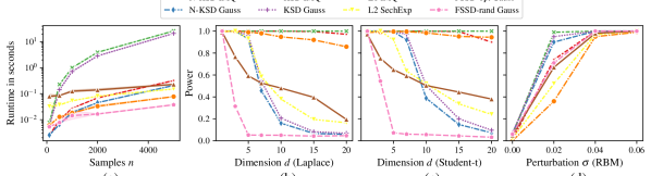
Restricted Boltzmann machine (RBM). Similar to Liu and Wang [2016], Jitkrittum et al. [2017], we consider the case where the target $\mathbb{P}$ is the non-normalized density of an RBM; the samples $\hat{\mathbb{Q}}_{n}$ are obtained from the same RBM perturbed by independent Gaussian noise with variance $\sigma^{2}$. For $\sigma^{2}=0$, $H_{0}:\mathbb{Q}=\mathbb{P}$ holds, and for $\sigma^{2}>0$, implying that the alternative $H_{1}:\mathbb{Q}\neq\mathbb{P}$ holds, the goal is to detect that the $n=1000$ samples come from a forged RBM. For the IMQ kernel (L1 IMQ, N-KSD IMQ, KSD IMQ), we set $c=1$ and $\beta=-1/2$. We show the results in Figure 1(d), using $100$ repetitions to obtain the power. KSD with the IMQ and with the Gaussian kernel performs best. Our proposed Nyström-based method ($m=4\sqrt{n}$) nearly matches its performance with both kernels while requiring only a fraction of the runtime. All other approaches achieve less power for $\sigma\in\{0.02,0.04\}$.

These experiments demonstrate the efficiency of the proposed Nyström-KSD method.

Acknowledgements

This work was supported by the pilot program Core-Informatics of the Helmholtz Association (HGF). BKS is partially supported by the National Science Foundation (NSF) CAREER award DMS-1945396.

References

  • Anastasiou et al. [2023] Andreas Anastasiou, Alessandro Barp, François-Xavier Briol, Bruno Ebner, Robert E Gaunt, Fatemeh Ghaderinezhad, Jackson Gorham, Arthur Gretton, Christophe Ley, Qiang Liu, et al. Stein’s method meets computational statistics: A review of some recent developments. Statistical Science, 38(1):120–139, 2023.
  • Antonini [1997] Rita Giuliano Antonini. Subgaussian random variables in Hilbert spaces. Rendiconti del Seminario Matematico della Università di Padova, 98:89–99, 1997.
  • Aronszajn [1950] Nachman Aronszajn. Theory of reproducing kernels. Transactions of the American Mathematical Society, 68:337–404, 1950.
  • Bardenet et al. [2014] Rémi Bardenet, Arnaud Doucet, and Christopher C. Holmes. Towards scaling up Markov chain Monte Carlo: an adaptive subsampling approach. In International Conference on Machine Learning (ICML), pages 405–413, 2014.
  • Baringhaus and Franz [2004] Ludwig Baringhaus and Carsten Franz. On a new multivariate two-sample test. Journal of Multivariate Analysis, 88:190–206, 2004.
  • Baringhaus and Henze [1988] Ludwig Baringhaus and Norbert Henze. A consistent test for multivariate normality based on the empirical characteristic function. Metrika. International Journal for Theoretical and Applied Statistics, 35(6):339–348, 1988.
  • Baum et al. [2023] Jerome Baum, Heishiro Kanagawa, and Arthur Gretton. A kernel Stein test of goodness of fit for sequential models. In International Conference on Machine Learning (ICML), pages 1936–1953, 2023.
  • Berlinet and Thomas-Agnan [2004] Alain Berlinet and Christine Thomas-Agnan. Reproducing Kernel Hilbert Spaces in Probability and Statistics. Kluwer, 2004.
  • Canonne [2021] Clément Canonne. Tail bounds for maximum of sub-Gaussian random variables. Mathematics Stack Exchange, 2021. https://math.stackexchange.com/q/4002713 (version: 2023-12-21).
  • Chatalic et al. [2022] Antoine Chatalic, Nicolas Schreuder, Alessandro Rudi, and Lorenzo Rosasco. Nyström kernel mean embeddings. In International Conference on Machine Learning (ICML), pages 3006–3024, 2022.
  • Chen [2021] Louis H. Y. Chen. Stein’s method of normal approximation: Some recollections and reflections. The Annals of Statistics, 49(4):1850–1863, 2021.
  • Chen et al. [2018] Wilson Ye Chen, Lester Mackey, Jackson Gorham, Francois-Xavier Briol, and Chris J. Oates. Stein points. In International Conference on Machine Learning (ICML), pages 844–853, 2018.
  • Chen et al. [2019] Wilson Ye Chen, Alessandro Barp, Francois-Xavier Briol, Jackson Gorham, Mark Girolami, Lester Mackey, and Chris Oates. Stein point Markov chain Monte Carlo. In International Conference on Machine Learning (ICML), pages 1011–1021, 2019.
  • Chwialkowski et al. [2015] Kacper Chwialkowski, Aaditya Ramdas, Dino Sejdinovic, and Arthur Gretton. Fast two-sample testing with analytic representations of probability measures. In Advances in Neural Information Processing Systems (NeurIPS), pages 1972–1980, 2015.
  • Chwialkowski et al. [2016] Kacper Chwialkowski, Heiko Strathmann, and Arthur Gretton. A kernel test of goodness of fit. In International Conference on Machine Learning (ICML), pages 2606–2615, 2016.
  • Coullon et al. [2023] Jeremie Coullon, Leah F. South, and Christopher Nemeth. Efficient and generalizable tuning strategies for stochastic gradient MCMC. Statistics and Computing, 33(3):66, 2023.
  • Della Vecchia et al. [2021] Andrea Della Vecchia, Jaouad Mourtada, Ernesto De Vito, and Lorenzo Rosasco. Regularized ERM on random subspaces. In International Conference on Artificial Intelligence and Statistics (AISTATS), pages 4006–4014, 2021.
  • Diestel and Uhl [1977] Joseph Diestel and John Jerry Uhl. Vector Measures. American Mathematical Society, 1977.
  • Fernandez et al. [2020] Tamara Fernandez, Nicolas Rivera, Wenkai Xu, and Arthur Gretton. Kernelized Stein discrepancy tests of goodness-of-fit for time-to-event data. In International Conference on Machine Learning (ICML), pages 3112–3122, 2020.
  • Fukuda [1990] Ryoji Fukuda. Exponential integrability of sub-Gaussian vectors. Probability Theory and Related Fields, 85(4):505–521, 1990.
  • Futami et al. [2019] Futoshi Futami, Zhenghang Cui, Issei Sato, and Masashi Sugiyama. Bayesian posterior approximation via greedy particle optimization. In AAAI Conference on Artificial Intelligence, pages 3606–3613, 2019.
  • Garreau et al. [2018] Damien Garreau, Wittawat Jitkrittum, and Motonobu Kanagawa. Large sample analysis of the median heuristic. Technical report, 2018. https://arxiv.org/abs/1707.07269.
  • Giorgobiani et al. [2020] George Giorgobiani, Vakhtang Kvaratskhelia, and Vaja Tarieladze. Notes on sub-Gaussian random elements. In Applications of Mathematics and Informatics in Natural Sciences and Engineering (AMINSE), pages 197–203, 2020.
  • Gorham and Mackey [2015] Jackson Gorham and Lester Mackey. Measuring sample quality with Stein’s method. In Advances in Neural Information Processing Systems (NeurIPS), pages 226–234, 2015.
  • Gorham and Mackey [2017] Jackson Gorham and Lester Mackey. Measuring sample quality with kernels. In International Conference on Machine Learning (ICML), pages 1292–1301, 2017.
  • Gorham et al. [2020] Jackson Gorham, Anant Raj, and Lester Mackey. Stochastic Stein discrepancies. In Advances in Neural Information Processing Systems (NeurIPS), pages 17931–17942, 2020.
  • Gretton et al. [2012] Arthur Gretton, Karsten Borgwardt, Malte Rasch, Bernhard Schölkopf, and Alexander Smola. A kernel two-sample test. Journal of Machine Learning Research, 13(25):723–773, 2012.
  • Hagrass et al. [2024] Omar Hagrass, Bharath Sriperumbudur, and Krishnakumar Balasubramanian. Minimax optimal goodness-of-fit testing with kernel Stein discrepancy. Technical report, 2024. https://arxiv.org/abs/2404.08278.
  • Huggins and Mackey [2018] Jonathan H. Huggins and Lester Mackey. Random feature Stein discrepancies. In Advances in Neural Information Processing Systems (NeurIPS), pages 1899–1909, 2018.
  • Ingster and Suslina [2003] Yuri I. Ingster and Irina A. Suslina. Nonparametric goodness-of-fit testing under Gaussian models. Springer, 2003.
  • Izzatullah et al. [2020] Muhammad Izzatullah, Ricardo Baptista, Lester Mackey, Youssef Marzouk, and Daniel Peter. Bayesian seismic inversion: Measuring Langevin MCMC sample quality with kernels. In SEG International Exposition and Annual Meeting, 2020.
  • Jitkrittum et al. [2017] Wittawat Jitkrittum, Wenkai Xu, Zoltán Szabó, Kenji Fukumizu, and Arthur Gretton. A linear-time kernel goodness-of-fit test. In Advances in Neural Information Processing Systems (NeurIPS), pages 262–271, 2017.
  • Jitkrittum et al. [2020] Wittawat Jitkrittum, Heishiro Kanagawa, and Bernhard Schölkopf. Testing goodness of fit of conditional density models with kernels. In Conference on Uncertainty in Artificial Intelligence (UAI), pages 221–230, 2020.
  • Kalinke and Szabó [2023] Florian Kalinke and Zoltán Szabó. Nyström M-Hilbert-Schmidt independence criterion. In Conference on Uncertainty in Artificial Intelligence (UAI), pages 1005–1015, 2023.
  • Koller and Friedman [2009] Daphne Koller and Nir Friedman. Probabilistic graphical models. MIT Press, 2009.
  • Kolmogorov [1933] Andrey N. Kolmogorov. Sulla determinazione empirica delle leggi di probabilita. Giornale dell’Istituto Italiano degli Attuari, 4(1), 1933.
  • Koltchinskii and Lounici [2017] Vladimir Koltchinskii and Karim Lounici. Concentration inequalities and moment bounds for sample covariance operators. Bernoulli, 23(1):110–133, 2017.
  • Korattikara et al. [2014] Anoop Korattikara, Yutian Chen, and Max Welling. Austerity in MCMC land: Cutting the Metropolis-Hastings budget. In International Conference on Machine Learning (ICML), pages 181–189, 2014.
  • Lehmann and Romano [2021] Erich L. Lehmann and Joseph P. Romano. Testing statistical hypotheses. Springer, 2021.
  • Lim et al. [2019] Jen Ning Lim, Makoto Yamada, Bernhard Schölkopf, and Wittawat Jitkrittum. Kernel Stein tests for multiple model comparison. In Advances in Neural Information Processing Systems (NeurIPS), pages 2243–2253, 2019.
  • Liu and Wang [2016] Qiang Liu and Dilin Wang. Stein variational gradient descent: A general purpose Bayesian inference algorithm. In Advances in Neural Information Processing Systems (NeurIPS), pages 2378–2386, 2016.
  • Liu et al. [2016] Qiang Liu, Jason Lee, and Michael Jordan. A kernelized Stein discrepancy for goodness-of-fit tests. In International Conference on Machine Learning (ICML), pages 276–284, 2016.
  • Martinez-Taboada and Kennedy [2023] Diego Martinez-Taboada and Edward H Kennedy. Counterfactual density estimation using kernel Stein discrepancies. Technical report, 2023. https://arxiv.org/abs/2309.16129.
  • Muandet et al. [2017] Krikamol Muandet, Kenji Fukumizu, Bharath Sriperumbudur, Bernhard Schölkopf, et al. Kernel mean embedding of distributions: A review and beyond. Foundations and Trends in Machine Learning, 10(1-2):1–141, 2017.
  • Nalisnick et al. [2019] Eric T. Nalisnick, Akihiro Matsukawa, Yee Whye Teh, and Balaji Lakshminarayanan. Detecting out-of-distribution inputs to deep generative models using a test for typicality. Technical report, 2019. http://arxiv.org/abs/1906.02994.
  • Oates et al. [2017] Chris J. Oates, Mark Girolami, and Nicolas Chopin. Control functionals for Monte Carlo integration. Journal of the Royal Statistical Society: Series B, 79(3):695–718, 2017.
  • Rahimi and Recht [2007] Ali Rahimi and Benjamin Recht. Random features for large-scale kernel machines. In Advances in Neural Information Processing Systems (NeurIPS), pages 1177–1184, 2007.
  • Rudi et al. [2015] Alessandro Rudi, Raffaello Camoriano, and Lorenzo Rosasco. Less is more: Nyström computational regularization. In Advances in Neural Information Processing Systems (NeurIPS), pages 1657–1665, 2015.
  • Salakhutdinov [2015] Ruslan Salakhutdinov. Learning deep generative models. Annual Review of Statistics and Its Application, 2:361–385, 2015.
  • Sarvmaili et al. [2024] Mahtab Sarvmaili, Hassan Sajjad, and Ga Wu. Data-centric prediction explanation via kernelized Stein discrepancy. Technical report, 2024. https://arxiv.org/abs/2403.15576.
  • Sejdinovic et al. [2013] Dino Sejdinovic, Bharath Sriperumbudur, Arthur Gretton, and Kenji Fukumizu. Equivalence of distance-based and RKHS-based statistics in hypothesis testing. Annals of Statistics, 41:2263–2291, 2013.
  • Smirnov [1948] Nikolai V. Smirnov. Table for estimating the goodness of fit of empirical distributions. Annals of Mathematical Statistics, 19:279–281, 1948.
  • Smola et al. [2007] Alexander Smola, Arthur Gretton, Le Song, and Bernhard Schölkopf. A Hilbert space embedding for distributions. In Algorithmic Learning Theory (ALT), pages 13–31, 2007.
  • Sriperumbudur and Sterge [2022] Bharath K. Sriperumbudur and Nicholas Sterge. Approximate kernel PCA: computational versus statistical trade-off. The Annals of Statistics, 50(5):2713–2736, 2022.
  • Stein [1972] Charles Stein. A bound for the error in the normal approximation to the distribution of a sum of dependent random variables. In Berkeley Symposium on Mathematical Statistics and Probability, pages 583–602, 1972.
  • Steinwart and Christmann [2008] Ingo Steinwart and Andreas Christmann. Support Vector Machines. Springer, 2008.
  • Sterge and Sriperumbudur [2022] Nicholas Sterge and Bharath K. Sriperumbudur. Statistical optimality and computational efficiency of Nyström kernel PCA. Journal of Machine Learning Research, 23(337):1–32, 2022.
  • Székely and Rizzo [2004] Gábor Székely and Maria Rizzo. Testing for equal distributions in high dimension. InterStat, 5:1249–1272, 2004.
  • Székely and Rizzo [2005] Gábor Székely and Maria Rizzo. A new test for multivariate normality. Journal of Multivariate Analysis, 93:58–80, 2005.
  • Talagrand [1987] Michel Talagrand. Regularity of Gaussian processes. Acta Mathematica, 159(1-2):99–149, 1987.
  • van der Vaart and Wellner [1996] Aad van der Vaart and Jon Wellner. Weak Convergence and Empirical Processes: With Applications to Statistics. Springer, 1996.
  • Vershynin [2018] Roman Vershynin. High-Dimensional Probability. Cambridge University Press, 2018.
  • Welling and Teh [2011] Max Welling and Yee Whye Teh. Bayesian learning via stochastic gradient Langevin dynamics. In International Conference on Machine Learning (ICML), pages 681–688, 2011.
  • Williams and Seeger [2001] Christopher Williams and Matthias Seeger. Using the Nyström method to speed up kernel machines. In Advances in Neural Information Processing Systems (NeurIPS), pages 682–688, 2001.
  • Wynne et al. [2024] George Wynne, Mikołaj Kasprzak, and Andrew B Duncan. A spectral representation of kernel Stein discrepancy with application to goodness-of-fit tests for measures on infinite dimensional Hilbert spaces. Bernoulli, 2024. (to appear).
  • Xu and Reinert [2021] Wenkai Xu and Gesine Reinert. A Stein goodness-of-test for exponential random graph models. In International Conference on Artificial Intelligence and Statistics (AISTATS), pages 415–423, 2021.
  • Yang et al. [2018] Jiasen Yang, Qiang Liu, Vinayak Rao, and Jennifer Neville. Goodness-of-fit testing for discrete distributions via Stein discrepancy. In International Conference on Machine Learning (ICML), pages 5561–5570, 2018.
  • Yang et al. [2019] Jiasen Yang, Vinayak A. Rao, and Jennifer Neville. A Stein-Papangelou goodness-of-fit test for point processes. In International Conference on Artificial Intelligence and Statistics (AISTATS), pages 226–235, 2019.
  • Yurinsky [1995] Vadim Yurinsky. Sums and Gaussian vectors. Springer, 1995.

Appendix A Proofs

This section is dedicated to the proofs of our results in the main text. Lemma 1 is proved in Section A.1. We prove our main result (Theorem 2) in Section A.2; Corollary 1 is shown in Section A.3.

A.1 Proof of Lemma 1

By (5), KSD is the norm of the mean embedding of $\mathbb{Q}$ under $h_{p}\left(\cdot,{\cdot}\right)$, that is,

$\displaystyle S_{p}(\mathbb{Q})=\left\|{\int_{\mathbb{R}^{d}}h_{p}\left(\cdot,{\mathbf{x}}\right)\mathrm{d}\mathbb{Q}(\mathbf{x})}\right\|_{\mathcal{H}_{h_{p}}}=\left\|{\mu_{h_{p}}(\mathbb{Q})}\right\|_{\mathcal{H}_{h_{p}}}.$ (A.1)

Hence, with Chatalic et al. [2022, (5)], the optimization problem (10) has the solution $\bm{\alpha}=(\alpha_{i})_{i=1}^{m}=\frac{1}{n}\mathbf{K}_{h_{p},m,m}^{-}\mathbf{K}_{h_{p},m,n}\bm{1}_{n}\in\mathbb{R}^{m}$. Now, using (A.1), we have

$\displaystyle\left\|{\sum_{i=1}^{m}\alpha_{i}h_{p}\left(\cdot,{\tilde{\mathbf{x}}_{i}}\right)}\right\|_{\mathcal{H}_{h_{p},m}}^{2}\stackrel{{\scriptstyle(a)}}{{=}}\left\langle\sum_{i=1}^{m}\alpha_{i}h_{p}\left(\cdot,{\tilde{\mathbf{x}}_{i}}\right),\sum_{i=1}^{m}\alpha_{i}h_{p}\left(\cdot,{\tilde{\mathbf{x}}_{i}}\right)\right\rangle_{\mathcal{H}_{h_{p},m}}$
$\displaystyle\stackrel{{\scriptstyle(b)}}{{=}}\sum_{i=1}^{m}\sum_{j=1}^{m}\alpha_{i}\alpha_{j}\left\langle h_{p}\left(\cdot,{\tilde{\mathbf{x}}_{i}}\right),h_{p}\left(\cdot,{\tilde{\mathbf{x}}_{j}}\right)\right\rangle_{\mathcal{H}_{h_{p},m}}\stackrel{{\scriptstyle(c)}}{{=}}\sum_{i=1}^{m}\sum_{j=1}^{m}\alpha_{i}\alpha_{j}h_{p}\left(\tilde{\mathbf{x}}_{i},\tilde{\mathbf{x}}_{j}\right)\stackrel{{\scriptstyle(d)}}{{=}}\bm{\alpha}^{\mkern-1.5mu\mathsf{T}}\mathbf{K}_{h_{p},m,m}\bm{\alpha}$
$\displaystyle\stackrel{{\scriptstyle(e)}}{{=}}\frac{1}{n^{2}}\bm{1}_{n}^{\mkern-1.5mu\mathsf{T}}\mathbf{K}_{h_{p},n,m}\underbrace{\mathbf{K}_{h_{p},m,m}^{-}\mathbf{K}_{h_{p},m,m}\mathbf{K}_{h_{p},m,m}^{-}}_{=\mathbf{K}_{h_{p},m,m}^{-}}\mathbf{K}_{h_{p},m,n}\bm{1}_{n}=\bm{\beta}_{p}^{\mkern-1.5mu\mathsf{T}}\mathbf{K}_{h_{p},m,m}^{-}\bm{\beta}_{p}.$

In (a) we used that $\left\|\cdot\right\|_{\mathcal{H}_{h_{p},m}}$ is inner product induced, (b) follows from the linearity of the inner product, (c) is implied by the reproducing property, (d) is by the definition the Gram matrix, in (e) we made use of the explicit form of $\bm{\alpha}$, the symmetry of Gram matrices, the property $\mathbf{K}_{h_{p},m,n}^{\mkern-1.5mu\mathsf{T}}=\mathbf{K}_{h_{p},n,m}$, and that the Moore-Penrose inverse satisfies $\mathbf{A}^{-}\mathbf{A}\mathbf{A}^{-}=\mathbf{A}^{-}$ for any matrix $\mathbf{A}$.

A.2 Proof of Theorem 2

Contrasting the existing related work [Rudi et al., 2015, Chatalic et al., 2022, Sterge and Sriperumbudur, 2022, Kalinke and Szabó, 2023], we do not impose a boundedness assumption on the feature map. This relaxation leads to new technical difficulties that we resolve in the following. Still, we start our analysis from a known decomposition Chatalic et al. [2022, Lemma 4.1].

To simplify notation, let $\mu_{h_{p}}:=\mu_{h_{p}}(\mathbb{Q})$, $\hat{\mu}_{h_{p}}:=\mu_{h_{p}}\left(\hat{\mathbb{Q}}_{n}\right)$, and $\hat{\mu}_{h_{p}}^{\text{Nys}}:=P_{\mathcal{H}_{h_{p},m}}\mu_{h_{p}}\left(\hat{\mathbb{Q}}_{n}\right)$. First, we decompose the error as follows.

$\displaystyle\left|S_{p}(\mathbb{Q})-\tilde{S}_{p}\left(\hat{\mathbb{Q}}_{n}\right)\right|\stackrel{{\scriptstyle(a)}}{{=}}\left|\left\|{\mu_{h_{p}}}\right\|_{\mathcal{H}_{h_{p}}}-\left\|{\hat{\mu}_{h_{p}}^{\text{Nys}}}\right\|_{\mathcal{H}_{h_{p}}}\right|\stackrel{{\scriptstyle(b)}}{{\leq}}\left\|{\mu_{h_{p}}-\hat{\mu}_{h_{p}}^{\text{Nys}}}\right\|_{\mathcal{H}_{h_{p}}}$ (A.2)
$\displaystyle\stackrel{{\scriptstyle(c)}}{{\leq}}\left\|{\mu_{h_{p}}-\hat{\mu}_{h_{p}}}\right\|_{\mathcal{H}_{h_{p}}}+\left\|{\hat{\mu}_{h_{p}}-\hat{\mu}_{h_{p}}^{\text{Nys}}}\right\|_{\mathcal{H}_{h_{p}}}$ (A.3)
$\displaystyle\stackrel{{\scriptstyle(d)}}{{=}}\left\|{\mu_{h_{p}}-\hat{\mu}_{h_{p}}}\right\|_{\mathcal{H}_{h_{p}}}+\left\|{\left(I-P_{\mathcal{H}_{h_{p},m}}\right)\left(\hat{\mu}_{h_{p}}-\frac{1}{m}\sum_{i=1}^{m}h_{p}\left(\cdot,{\tilde{\mathbf{x}}_{i}}\right)\right)}\right\|_{\mathcal{H}_{h_{p}}}$ (A.4)
$\displaystyle\stackrel{{\scriptstyle(e)}}{{\leq}}\underbrace{\left\|{\mu_{h_{p}}-\hat{\mu}_{h_{p}}}\right\|_{\mathcal{H}_{h_{p}}}}_{=:t_{1}}+\underbrace{\left\|{\left(I-P_{\mathcal{H}_{h_{p},m}}\right)C_{\mathbb{Q},h_{p},\lambda}^{1/2}}\right\|_{\mathrm{op}}}_{=:t_{2}}\underbrace{\left\|{C_{\mathbb{Q},h_{p},\lambda}^{-1/2}\left(\hat{\mu}_{h_{p}}-\frac{1}{m}\sum_{i=1}^{m}h_{p}\left(\cdot,{\tilde{\mathbf{x}}_{i}}\right)\right)}\right\|_{\mathcal{H}_{h_{p}}}}_{=:t_{3}}.$ (A.5)

(a) is implied by (A.1) and (11); (b) follows from the reverse triangle inequality; $\pm\hat{\mu}_{h_{p}}$ and the triangle inequality yield (c); in (d), we use the distributive property and introduce $\frac{1}{m}\sum_{i=1}^{m}h_{p}\left(\cdot,{\tilde{\mathbf{x}}_{i}}\right)\in\mathcal{H}_{h_{p},m}$ whose projection onto the orthogonal complement of $\mathcal{H}_{h_{p},m}$ is zero; in (e) $I=C_{\mathbb{Q},h_{p},\lambda}^{1/2}C_{\mathbb{Q},h_{p},\lambda}^{-1/2}$ was introduced and we used the definition of the operator norm.

We next obtain individual probabilistic bounds for the three terms $t_{1}$, $t_{2}$, and $t_{3}$, which we subsequently combine by union bound. We will then conclude the proof by showing that all assumptions that we imposed along the way are satisfied.

  • Term $t_{1}$. The first term measures the deviation of an empirical mean $\hat{\mu}_{h_{p}}$ to its population counterpart $\mu_{h_{p}}$. To bound this deviation $\left\|{\hat{\mu}_{h_{p}}-\mu_{h_{p}}}\right\|_{\mathcal{H}_{h_{p}}}=\Big{\|}\frac{1}{n}\sum_{i=1}^{n}[h_{p}\left(\cdot,{\mathbf{x}_{i}}\right)-\underbrace{\mathbb{E}_{X\sim\mathbb{Q}}h_{p}\left(\cdot,{X}\right)}_{=0}]\Big{\|}_{\mathcal{H}_{h_{p}}}$, we will use the Bernstein inequality (Theorem D.4) with the $\eta_{i}:=h_{p}\left(\cdot,{\mathbf{x}_{i}}\right)\in\mathcal{H}_{h_{p}}$ $(i\in[n])$ centered random variables, by gaining control on the moments of $Y:=\left\|h_{p}(\cdot,X)\right\|_{\mathcal{H}_{h_{p}}}$. This is what we elaborate next.

    By Assumption 1(ii), $Y$ is sub-Gaussian; hence it is also sub-exponential (Lemma D.2(3)), and therefore (Lemma B.2) it satisfies the Bernstein condition

    $\displaystyle\mathbb{E}|Y|^{p}$ $\displaystyle\leq\frac{1}{2}p!\sigma^{2}B^{p-2}<\infty,\quad\text{with}$ $\displaystyle\sigma$ $\displaystyle=\sqrt{2}\left\|{Y}\right\|_{\psi_{1}},$ $\displaystyle B$ $\displaystyle=\left\|{Y}\right\|_{\psi_{1}},$ (A.6)

    for any $p\geq 2$. Notice that

    $\displaystyle B$ $\displaystyle=\left\|{Y}\right\|_{\psi_{1}}\stackrel{{\scriptstyle(a)}}{{\lesssim}}\left\|{Y}\right\|_{\psi_{2}}\stackrel{{\scriptstyle(b)}}{{\lesssim}}\left\|{Y}\right\|_{L_{2}(\mathbb{Q})}\stackrel{{\scriptstyle(c)}}{{=}}\left(\mathbb{E}_{X\sim\mathbb{Q}}\left\|h_{p}(\cdot,X)\right\|_{\mathcal{H}_{h_{p}}}^{2}\right)^{1/2}$ (A.7)
    $\displaystyle\stackrel{{\scriptstyle(d)}}{{=}}\left[\mathbb{E}_{X\sim\mathbb{Q}}\operatorname{tr}\left(h_{p}\left(\cdot,{X}\right)\otimes h_{p}\left(\cdot,{X}\right)\right)\right]^{1/2}\stackrel{{\scriptstyle(e)}}{{=}}\sqrt{\operatorname{tr}\left(C_{\mathbb{Q},h_{p}}\right)},$ (A.8)

    (a) follows from Lemma D.2(3), (b) is implied by Assumption 1(ii), (c) comes from the definition of $Y$, in (d) we used Lemma D.1. Steinwart and Christmann [2008, (A.32)] allows commuting $\operatorname{tr}$ and integration, which, with (1), yields (e). As $\sigma\asymp B$, we also got that $\sigma\lesssim\sqrt{\operatorname{tr}\left(C_{\mathbb{Q},h_{p}}\right)}$.

    Having obtained a bound on the moments, we can apply Bernstein’s inequality for separable Hilbert spaces (Yurinsky 1995; recalled in Theorem D.4) to the centered $\eta_{i}=h_{p}\left(\cdot,{\mathbf{x}_{i}}\right)\in\mathcal{H}_{h_{p}}$-s ($i\in[n]$), and obtain that for any $\delta\in(0,1)$ it holds with probability at least $1-\delta/3$ that

    $\displaystyle\left\|{\mu_{h_{p}}-\hat{\mu}_{h_{p}}}\right\|_{\mathcal{H}_{h_{p}}}=\left\|{\frac{1}{n}\sum_{i=1}^{n}\eta_{i}}\right\|_{\mathcal{H}_{h_{p}}}\lesssim\frac{\sqrt{\operatorname{tr}\left(C_{\mathbb{Q},h_{p}}\right)}\log(6/\delta)}{n}+\sqrt{\frac{\operatorname{tr}\left(C_{\mathbb{Q},h_{p}}\right)\log(6/\delta)}{n}}.$ (A.10)
  • Term $t_{2}$. Assume that $0<\lambda\leq\left\|{C_{\mathbb{Q},h_{p}}}\right\|_{\mathrm{op}}$. Then, we can handle the second term with Lemma B.1 and obtain that for any $\delta\in(0,1)$ it holds with probability at least $1-\delta/3$ that

    $\displaystyle\left\|{\left(I-P_{\mathcal{H}_{h_{p},m}}\right)C_{\mathbb{Q},h_{p},\lambda}^{1/2}}\right\|_{\mathrm{op}}\lesssim\sqrt{\lambda}$ (A.11)

    provided that $m\gtrsim\max\left\{\frac{\operatorname{tr}\left(C_{\mathbb{Q},h_{p}}\right)}{\lambda},\log(3/\delta)\right\}$.

  • Term $t_{3}$. The third term depends on the sample $(\mathbf{x}_{i})_{i=1}^{n}\stackrel{{\scriptstyle\text{i.i.d.}}}{{\sim}}\mathbb{Q}$ and on the Nyström selection $(i_{j})_{j=1}^{m}\stackrel{{\scriptstyle\text{i.i.d.}}}{{\sim}}\text{Unif}([n])=:\Lambda$; with this notation $\tilde{\mathbf{x}}_{j}=\mathbf{x}_{i_{j}}$ ($j\in[m]$). Our goal is to take both sources of randomness into account.

    Fixed $\mathbf{x}_{i}$-s, randomness in $i_{j}$-s: Let the sample $(\mathbf{x}_{i})_{i=1}^{n}$ be fixed. As the $(\mathbf{x}_{i_{j}})_{j=1}^{m}$-s are i.i.d.,

    $\displaystyle t_{3}$ $\displaystyle=\Bigg{\|}C_{\mathbb{Q},h_{p},\lambda}^{-1/2}\left(\hat{\mu}_{h_{p}}-\frac{1}{m}\sum_{i=1}^{m}h_{p}\left(\cdot,{\tilde{\mathbf{x}}_{i}}\right)\right)\Bigg{\|}_{\mathcal{H}_{h_{p}}}$ $\displaystyle=\Bigg{\|}\frac{1}{m}\sum_{i=1}^{m}\underbrace{\left[C_{\mathbb{Q},h_{p},\lambda}^{-1/2}\left(h_{p}\left(\cdot,{\tilde{\mathbf{x}}_{i}}\right)-\hat{\mu}_{h_{p}}\right)\right]}_{:=Y_{i}}\Bigg{\|}_{\mathcal{H}_{h_{p}}}$ (A.12)

    measures the concentration of the sum $\frac{1}{m}\sum_{i=1}^{m}Y_{i}$ around its expectation, which is zero as $\mathbb{E}_{J}\left[h_{p}(\cdot,\mathbf{x}_{J})\right]=\hat{\mu}_{h_{p}}$ with $J\sim\Lambda$. Notice that

    $\displaystyle\max_{i\in[m]}\left\|{Y_{i}}\right\|_{\mathcal{H}_{h_{p}}}$ $\displaystyle=\max_{i\in[m]}\left\|{C_{\mathbb{Q},h_{p},\lambda}^{-1/2}\left(h_{p}\left(\cdot,{\tilde{\mathbf{x}}_{i}}\right)-\hat{\mu}_{h_{p}}\right)}\right\|_{\mathcal{H}_{h_{p}}}$ (A.13)
    $\displaystyle\leq\max_{i\in[m]}\left[\left\|{C_{\mathbb{Q},h_{p},\lambda}^{-1/2}h_{p}(\cdot,\tilde{\mathbf{x}}_{i})}\right\|_{\mathcal{H}_{h_{p}}}+\frac{1}{n}\sum_{j=1}^{n}\left\|{C_{\mathbb{Q},h_{p},\lambda}^{-1/2}h_{p}(\cdot,\mathbf{x}_{j})}\right\|_{\mathcal{H}_{h_{p}}}\right]$ (A.14)
    $\displaystyle\leq 2\max_{i\in[n]}\left\|{C_{\mathbb{Q},h_{p},\lambda}^{-1/2}h_{p}\left(\cdot,{\mathbf{x}_{i}}\right)}\right\|_{\mathcal{H}_{h_{p}}}=:K=K(\mathbf{x}_{1},\ldots,\mathbf{x}_{n}),$ (A.15)

    where we used the triangle inequality and homogeneity of the norm. An application of Theorem D.5 yields that, conditioned on the sample $(\mathbf{x}_{i})_{i=1}^{n}$, it holds that

    $\displaystyle\Lambda^{m}\!\left((i_{j})_{j=1}^{m}\,:\,t_{3}\leq K\frac{\sqrt{2\log(12/\delta)}}{\sqrt{m}}\enspace\Bigg{|}\,\left(\mathbf{x}_{i}\right)_{i=1}^{n}\right)\geq 1-\frac{\delta}{6}.$ (A.16)

    Randomness in $\mathbf{x}_{i}$-s: Let $Z_{i}:=\left\|{C_{\mathbb{Q},h_{p},\lambda}^{-1/2}h_{p}\left(\cdot,{\mathbf{x}_{i}}\right)}\right\|_{\mathcal{H}_{h_{p}}}$ ($i\in[n]$) with $(\mathbf{x}_{i})_{i=1}^{n}\stackrel{{\scriptstyle\text{i.i.d.}}}{{\sim}}\mathbb{Q}$. By Assumption 1(ii) and Lemma B.3, the $Z_{i}$-s are sub-Gaussian random variable provided that $0<\lambda\leq\left\|{C_{\mathbb{Q},h_{p}}}\right\|_{\mathrm{op}}$. Hence, by Lemma B.6, with probability at least $1-\delta/6$, it holds that

    $\displaystyle K=2\max_{i\in[n]}|Z_{i}|\lesssim\sqrt{\left\|{Z_{1}}\right\|_{\psi_{2}}^{2}\log(12n/\delta)}.$ (A.17)

    We now bound $\left\|{Z_{1}}\right\|_{\psi_{2}}^{2}$:

    $\displaystyle\left\|{Z_{1}}\right\|_{\psi_{2}}^{2}\stackrel{{\scriptstyle(a)}}{{=}}\left\|{\left\|{C_{\mathbb{Q},h_{p},\lambda}^{-1/2}h_{p}\left(\cdot,{\mathbf{x}_{1}}\right)}\right\|_{\mathcal{H}_{h_{p}}}}\right\|_{\psi_{2}}^{2}\stackrel{{\scriptstyle(b)}}{{\lesssim}}\left\|{\left\|{C_{\mathbb{Q},h_{p},\lambda}^{-1/2}h_{p}\left(\cdot,{\mathbf{x}_{1}}\right)}\right\|_{\mathcal{H}_{h_{p}}}}\right\|_{L_{2}(\mathbb{Q})}^{2}\stackrel{{\scriptstyle(c)}}{{=}}\operatorname{tr}\left(C_{\mathbb{Q},h_{p},\lambda}^{-1}C_{\mathbb{Q},h_{p}}\right).$ (A.18)

    (a) follows from the definition of $Z_{1}$. (b) is implied by Assumption 1(ii) and Lemma B.3. (c) comes from Lemma B.4 with $A:=C_{\mathbb{Q},h_{p},\lambda}^{-1}$. We have shown that

    $\displaystyle\mathbb{Q}^{n}\!\left(\left(\mathbf{x}_{i}\right)_{i=1}^{n}\,:\,K\lesssim\sqrt{\operatorname{tr}\left(C_{\mathbb{Q},h_{p},\lambda}^{-1}C_{\mathbb{Q},h_{p}}\right)\log(12n/\delta)}\right)\geq 1-\frac{\delta}{6}.$ (A.19)

    Combination: We now combine the intermediate results. Let

    $\displaystyle A$ $\displaystyle=\left\{\left(\left(\mathbf{x}_{i}\right)_{i=1}^{n},\left(i_{j}\right)_{j=1}^{m}\right)\;:\;t_{3}\lesssim\frac{\sqrt{\operatorname{tr}\left(C_{\mathbb{Q},h_{p},\lambda}^{-1}C_{\mathbb{Q},h_{p}}\right)\log(12n/\delta)\log(12/\delta)}}{\sqrt{m}}\right\},$ (A.20)
    $\displaystyle B$ $\displaystyle=\left\{\left(\mathbf{x}_{i}\right)_{i=1}^{n}\,:\,K\lesssim\sqrt{\operatorname{tr}\left(C_{\mathbb{Q},h_{p},\lambda}^{-1}C_{\mathbb{Q},h_{p}}\right)\log(12n/\delta)}\right\},$ (A.21)
    $\displaystyle C$ $\displaystyle=\left\{\left(\left(\mathbf{x}_{i}\right)_{i=1}^{n},\left(i_{j}\right)_{j=1}^{m}\right)\;:\;t_{3}\leq K\frac{\sqrt{2\log(12/\delta)}}{\sqrt{m}}\right\}\subseteq A.$ (A.22)

    Then, with $\mathbb{Q}^{n}\otimes\Lambda^{m}$ denoting the product measure of $\mathbb{Q}^{n}$ and $\Lambda^{m}$, we obtain

    $\displaystyle\left(\mathbb{Q}^{n}\otimes\Lambda^{m}\right)\!\left(A\right)=\mathbb{E}_{\mathbb{Q}^{n}}\!\left[\Lambda^{m}\left(A\mid\left(\mathbf{x}_{i}\right)_{i=1}^{n}\right)\right]=\int_{\left(\mathbb{R}^{d}\right)^{n}}\Lambda^{m}\!\left(A\mid\left(\mathbf{x}_{i}\right)_{i=1}^{n}\right)\mathrm{d}\mathbb{Q}^{n}(\mathbf{x}_{1},\ldots,\mathbf{x}_{n})$ (A.23)
    $\displaystyle\geq\int_{B}\Lambda^{m}\!\left(A\mid\left(\mathbf{x}_{i}\right)_{i=1}^{n}\right)\mathrm{d}\mathbb{Q}^{n}(\mathbf{x}_{1},\ldots,\mathbf{x}_{n})\geq\int_{B}\Lambda^{m}\!\left(C\mid\left(\mathbf{x}_{i}\right)_{i=1}^{n}\right)\mathrm{d}\mathbb{Q}^{n}(\mathbf{x}_{1},\ldots,\mathbf{x}_{n})$ (A.24)
    $\displaystyle\stackrel{{\scriptstyle(a)}}{{\geq}}\left(1-\frac{\delta}{6}\right)\mathbb{Q}^{n}(B)\stackrel{{\scriptstyle(b)}}{{\geq}}(1-\delta/6)^{2}=1-\delta/3+\delta^{2}/6^{2}>1-\delta/3.$ (A.25)

    (a) is implied by the uniform lower bound established in (A.16). (b) was shown in (A.19).

Combination of $t_{1}$, $t_{2}$, and $t_{3}$.

To conclude, we use decomposition (A.5), and union bound (A.10), (A.11), and (A.25). Further, we observe that $\operatorname{tr}\left(C_{\mathbb{Q},h_{p},\lambda}^{-1}C_{\mathbb{Q},h_{p}}\right)=\mathcal{N}_{\mathbb{Q},h_{p}}(\lambda)$, and obtain that with probability at least $1-\delta$ it holds that

$\displaystyle\left|S_{p}(\mathbb{Q})-\tilde{S}_{p}\left(\hat{\mathbb{Q}}_{n}\right)\right|$ $\displaystyle\lesssim\frac{\sqrt{\operatorname{tr}\left(C_{\mathbb{Q},h_{p}}\right)}\log(6/\delta)}{n}+\sqrt{\frac{\operatorname{tr}\left(C_{\mathbb{Q},h_{p}}\right)\log(6/\delta)}{n}}+$ (A.26)
$\displaystyle\quad+\sqrt{\frac{\lambda\mathcal{N}_{\mathbb{Q},h_{p}}(\lambda)\log(12n/\delta)\log(12/\delta)}{m}}$ (A.27)

provided that $m\gtrsim\max\left\{\frac{\operatorname{tr}\left(C_{\mathbb{Q},h_{p}}\right)}{\lambda},\log(3/\delta)\right\}$ and $0<\lambda\leq\left\|{C_{\mathbb{Q},h_{p}}}\right\|_{\mathrm{op}}$ both hold. Now, specializing $\lambda=\frac{c\operatorname{tr}\left(C_{\mathbb{Q},h_{p}}\right)}{m}$ for some absolute constant $c>0$, all constraints are satisfied for $m\gtrsim\max\left\{\log(3/\delta),\operatorname{tr}\left(C_{\mathbb{Q},h_{p}}\right)\left\|{C_{\mathbb{Q},h_{p}}}\right\|_{\mathrm{op}}^{-1}\right\}$. Using our choice of $\lambda$, after rearranging, we get the stated claim.

A.3 Proof of Corollary 1

The proof is split into two parts. The first one considers the polynomial decay assumption, the second one is about the exponential decay assumption.

  • Polynomial decay. The $\sqrt{n}$-consistency of the first two addends in Theorem 2 was established in the discussion following the statement. Hence, we limit our considerations to the last addend. Assume that $\mathcal{N}_{\mathbb{Q},h_{p}}(\lambda)\lesssim\lambda^{-\gamma}$ for $\gamma\in(0,1]$. Observing that the trace expression is constant, the last addend in Theorem 2 yields that

    $\displaystyle\sqrt{\frac{\log(12/\delta)\log(12n/\delta)\mathcal{N}_{\mathbb{Q},h_{p}}\left(\frac{c\operatorname{tr}\left(C_{\mathbb{Q},h_{p}}\right)}{m}\right)}{m^{2}}}\stackrel{{\scriptstyle(a)}}{{\lesssim}}\sqrt{\frac{\log(12/\delta)\log(12n/\delta)}{m^{2-\gamma}}}\stackrel{{\scriptstyle(b)}}{{=}}\mathcal{O}\left(\frac{1}{\sqrt{n}}\right),$ (A.29)

    with (a) implied by the polynomial decay assumption and (b) follows from our choice of $m\gtrsim n^{\frac{1}{2-\gamma}}\log^{\frac{1}{2-\gamma}}(12n/\delta)\log^{\frac{1}{2-\gamma}}(12/\delta)$. This derivation confirms the first stated result.

  • Exponential decay. Assume it holds that $\mathcal{N}_{\mathbb{Q},h_{p}}(\lambda)\lesssim\log(1+c_{1}/\lambda)$. Observe that as per the discussion following Theorem 2, the first two addends are $\mathcal{O}\left(n^{-1/2}\right)$. For the last addend, again noticing that the trace is constant, we have

    $\displaystyle\sqrt{\frac{\log(12/\delta)\log(12n/\delta)\mathcal{N}_{\mathbb{Q},h_{p}}\!\left(\frac{c\operatorname{tr}\left(C_{\mathbb{Q},h_{p}}\right)}{m}\right)}{m^{2}}}\stackrel{{\scriptstyle(a)}}{{\lesssim}}\sqrt{\frac{\log(12/\delta)\log(12n/\delta)\log\left(1+\frac{c_{1}m}{c\operatorname{tr}\left(C_{\mathbb{Q},h_{p}}\right)}\right)}{m^{2}}}$ (A.30)
    $\displaystyle\stackrel{{\scriptstyle(b)}}{{\lesssim}}\sqrt{\frac{\log(12/\delta)\log(12n/\delta)\log\left(1+\frac{c_{1}n}{c\operatorname{tr}\left(C_{\mathbb{Q},h_{p}}\right)}\right)}{m^{2}}}\stackrel{{\scriptstyle(c)}}{{=}}\mathcal{O}\left(\frac{1}{\sqrt{n}}\right),$ (A.31)

    where (a) uses the exponential decay assumption. (b) uses that $n\geq m$ and that the logarithm is a monotonically increasing function. (c) follows from our choice of

    $\displaystyle m\gtrsim\sqrt{n}\sqrt{\log\left(1+\frac{c_{1}n}{c\operatorname{tr}\left(C_{\mathbb{Q},h_{p}}\right)}\right)\log(12n/\delta)\log(12/\delta)},$ (A.32)

    finishing the proof of the corollary.

Appendix B Auxiliary results

This section collects our auxiliary results. Lemma B.1 builds on Rudi et al. [2015, Lemma 6], which assumes bounded feature maps, and on Della Vecchia et al. [2021, Lemma 5], which is stated in the context of leverage scores. Lemma B.2 states that a sub-exponential random variable satisfies Bernstein’s conditions, and Lemma B.3 shows that a “whitened” sub-Gaussian vector remains sub-Gaussian. Lemma B.4 expresses the $L_{2}$-norm of the RKHS-norm as trace. In Lemma B.5, we show how tensor products interplay with linearly transformed vectors. Lemma B.6 is about the maximum of real-valued sub-Gaussian random variables; it is a slightly altered restatement of Canonne [2021].

Lemma B.1.

Let Assumption 1 hold, and assume $0<\lambda\leq\left\|{C_{\mathbb{Q},h_{p}}}\right\|_{\mathrm{op}}$. Then, for any $\delta\in(0,1)$, it holds with probability at least $1-\delta$ that

$\displaystyle\left\|{\left(I-P_{\mathcal{H}_{h_{p},m}}\right)C_{\mathbb{Q},h_{p},\lambda}^{1/2}}\right\|_{\mathrm{op}}^{2}\lesssim\lambda$ (B.33)

provided that $m\gtrsim\max\left\{\frac{\operatorname{tr}\left(C_{\mathbb{Q},h_{p}}\right)}{\lambda},\log(1/\delta)\right\}$.

Proof.

Let the covariance of the Nyström samples be $\tilde{C}_{\hat{\mathbb{Q}}_{n},h_{p},m}=\frac{1}{m}\sum_{i=1}^{m}h_{p}\left(\cdot,{\tilde{\mathbf{x}}_{i}}\right)\otimes h_{p}\left(\cdot,{\tilde{\mathbf{x}}_{i}}\right)$, and $\beta(\lambda)=\lambda_{\text{max}}\left(C_{\mathbb{Q},h_{p},\lambda}^{-1/2}\left(C_{\mathbb{Q},h_{p}}-\tilde{C}_{\hat{\mathbb{Q}}_{n},h_{p},m}\right)C_{\mathbb{Q},h_{p},\lambda}^{-1/2}\right)$. The application of Rudi et al. [2015, Proposition 3 and Proposition 7] (recalled in Theorem D.6) yields the non-probabilistic inequality

$\displaystyle\left\|{\left(I-P_{\mathcal{H}_{h_{p},m}}\right)C_{\mathbb{Q},h_{p},\lambda}^{1/2}}\right\|_{\mathrm{op}}^{2}\leq\frac{\lambda}{1-\beta(\lambda)},$ (B.34)

when $\beta(\lambda)<1$. $\beta(\lambda)$ measures the deviation—in the sense of $\lambda_{\text{max}}(\cdot)$—of an empirical covariance to the population one. We will establish that our setting satisfies the conditions of Koltchinskii and Lounici [2017, Theorem 9] (recalled in Theorem D.3), with which we will show that the stronger requirement

$\displaystyle\beta(\lambda)\stackrel{{\scriptstyle(a)}}{{\leq}}\left\|{C_{\mathbb{Q},h_{p},\lambda}^{-1/2}\left(C_{\mathbb{Q},h_{p}}-\tilde{C}_{\hat{\mathbb{Q}}_{n},h_{p},m}\right)C_{\mathbb{Q},h_{p},\lambda}^{-1/2}}\right\|_{\mathrm{op}}$ (B.35)
$\displaystyle\stackrel{{\scriptstyle(b)}}{{=}}\left\|{C_{\mathbb{Q},h_{p},\lambda}^{-1/2}C_{\mathbb{Q},h_{p}}C_{\mathbb{Q},h_{p},\lambda}^{-1/2}-C_{\mathbb{Q},h_{p},\lambda}^{-1/2}\tilde{C}_{\hat{\mathbb{Q}}_{n},h_{p},m}C_{\mathbb{Q},h_{p},\lambda}^{-1/2}}\right\|_{\mathrm{op}}$ (B.36)
$\displaystyle\stackrel{{\scriptstyle(c)}}{{=}}\left\|{\frac{1}{m}\sum_{i=1}^{m}C_{\mathbb{Q},h_{p},\lambda}^{-1/2}h_{p}\left(\cdot,{\tilde{\mathbf{x}}_{i}}\right)\otimes h_{p}\left(\cdot,{\tilde{\mathbf{x}}_{i}}\right)C_{\mathbb{Q},h_{p},\lambda}^{-1/2}-C_{\mathbb{Q},h_{p},\lambda}^{-1/2}C_{\mathbb{Q},h_{p}}C_{\mathbb{Q},h_{p},\lambda}^{-1/2}}\right\|_{\mathrm{op}}<1\hskip 28.45274pt$ (B.37)

is satisfied for $m$ large enough. In (a), we used that the spectral radius is bounded by the operator norm. (b) is the distributive property, and (c) uses linearity.

In the following we prove (B.37). Let the Nyström selection be $\left(i_{j}\right)_{j=1}^{m}\stackrel{{\scriptstyle\text{i.i.d.}}}{{\sim}}\text{Unif}([n])$; with this notation $\tilde{\mathbf{x}}_{j}=\mathbf{x}_{i_{j}}$ ($j\in[m])$. First, we condition on a fixed choice of $\left(i_{j}\right)_{j=1}^{m}$-s. Let us define the $Y=C_{\mathbb{Q},h_{p},\lambda}^{-1/2}h_{p}\left(\cdot,{X}\right)\in\mathcal{H}_{h_{p}}$ random variable with $X\sim\mathbb{Q}$, and consider the samples $y_{i_{j}}:=C_{\mathbb{Q},h_{p},\lambda}^{-1/2}h_{p}\left(\cdot,{\mathbf{x}_{i_{j}}}\right)\in\mathcal{H}_{h_{p}}$. $Y$ has covariance

$\displaystyle\mathbb{E}_{X\sim\mathbb{Q}}\left[Y\otimes Y\right]\stackrel{{\scriptstyle(a)}}{{=}}\mathbb{E}_{X\sim\mathbb{Q}}\left[C_{\mathbb{Q},h_{p},\lambda}^{-1/2}h_{p}\left(\cdot,{X}\right)\otimes h_{p}\left(\cdot,{X}\right)C_{\mathbb{Q},h_{p},\lambda}^{-1/2}\right]\stackrel{{\scriptstyle(b)}}{{=}}C_{\mathbb{Q},h_{p},\lambda}^{-1/2}C_{\mathbb{Q},h_{p}}C_{\mathbb{Q},h_{p},\lambda}^{-1/2},$ (B.38)

where (a) is implied by Lemma B.5 and (b) follows from Steinwart and Christmann [2008, (A.32)] by swapping the expectation with bounded linear operators. Similarly, we observe that the empirical covariance is $\frac{1}{m}\sum_{j=1}^{m}y_{i_{j}}\otimes y_{i_{j}}=C_{\mathbb{Q},h_{p},\lambda}^{-1/2}\tilde{C}_{\hat{\mathbb{Q}}_{n},h_{p},m}C_{\mathbb{Q},h_{p},\lambda}^{-1/2}$. In other words, this setup brings us into the setting of Theorem D.3, and it remains to show that $Y$ is sub-Gaussian in the sense of (2). Notice that $Y$ satisfies both conditions:

  • Mean-zero: By $\mathbb{P}=\mathbb{Q}$ and (6), $\mathbb{E}Y=C_{\mathbb{Q},h_{p},\lambda}^{-1/2}\mathbb{E}h_{p}\left(\cdot,{X}\right)=0$.

  • (2) holds: Our goal now is to show that $\left\|{\left\langle{Y,u}\right\rangle_{\mathcal{H}_{h_{p}}}}\right\|_{\psi_{2}}\lesssim\left\|{\left\langle{Y,u}\right\rangle_{\mathcal{H}_{h_{p}}}}\right\|_{L_{2}(\mathbb{Q})}<\infty$ holds for all $u\in\mathcal{H}_{h_{p}}$. Let $u\in\mathcal{H}_{h_{p}}$ be arbitrary, and $v=C_{\mathbb{Q},h_{p},\lambda}^{-1/2}u\in\mathcal{H}_{h_{p}}$; $v$ is well-defined due to the invertibility of $C_{\mathbb{Q},h_{p},\lambda}$. Using this notation, we have

    $\displaystyle\left\|{\left\langle{Y,u}\right\rangle_{\mathcal{H}_{h_{p}}}}\right\|_{\psi_{2}}\stackrel{{\scriptstyle(a)}}{{=}}\left\|{\left\langle{C_{\mathbb{Q},h_{p},\lambda}^{-1/2}h_{p}\left(\cdot,{X}\right),u}\right\rangle_{\mathcal{H}_{h_{p}}}}\right\|_{\psi_{2}}\stackrel{{\scriptstyle(b)}}{{=}}\left\|{\left\langle{h_{p}\left(\cdot,{X}\right),C_{\mathbb{Q},h_{p},\lambda}^{-1/2}u}\right\rangle_{\mathcal{H}_{h_{p}}}}\right\|_{\psi_{2}}$ (B.39)
    $\displaystyle\stackrel{{\scriptstyle(c)}}{{=}}\left\|{\left\langle{h_{p}\left(\cdot,{X}\right),v}\right\rangle_{\mathcal{H}_{h_{p}}}}\right\|_{\psi_{2}}\stackrel{{\scriptstyle(d)}}{{\lesssim}}\left\|{\left\langle{h_{p}\left(\cdot,{X}\right),v}\right\rangle_{\mathcal{H}_{h_{p}}}}\right\|_{L_{2}(\mathbb{Q})}\stackrel{{\scriptstyle(e)}}{{=}}\left\|{\left\langle{h_{p}\left(\cdot,{X}\right),C_{\mathbb{Q},h_{p},\lambda}^{-1/2}u}\right\rangle_{\mathcal{H}_{h_{p}}}}\right\|_{L_{2}(\mathbb{Q})}$ (B.40)
    $\displaystyle\stackrel{{\scriptstyle(f)}}{{=}}\left\|{\left\langle{C_{\mathbb{Q},h_{p},\lambda}^{-1/2}h_{p}\left(\cdot,{X}\right),u}\right\rangle_{\mathcal{H}_{h_{p}}}}\right\|_{L_{2}(\mathbb{Q})}\stackrel{{\scriptstyle(g)}}{{=}}\left\|{\left\langle{Y,u}\right\rangle_{\mathcal{H}_{h_{p}}}}\right\|_{L_{2}(\mathbb{Q})}\stackrel{{\scriptstyle(h)}}{{<}}\infty.$ (B.41)

    In (a), we use the definition of $Y$. (b) follows from the self-adjointness of $C_{\mathbb{Q},h_{p},\lambda}^{-1/2}$. (c) uses the definition of $v$. (d) is implied by Assumption 1(i) holding for all $v\in\mathcal{H}_{h_{p}}$. In (e) we again used the definition of $v$. (f) is implied by the self-adjointness of $C_{\mathbb{Q},h_{p},\lambda}^{-1/2}$. (g) is based on the definition of $Y$. (h) holds as $\left\|{\left\langle{h_{p}\left(\cdot,{X}\right),v}\right\rangle_{\mathcal{H}_{h_{p}}}}\right\|_{L_{2}(\mathbb{Q})}<\infty$ by Assumption 1(i) and the expressions in-between were equalities. This establishes the sub-Gaussianity of $Y$.

Now, we can invoke Koltchinskii and Lounici [2017, Theorem 9] (recalled in Theorem D.3), and, by using (B.37), we obtain that with probability at least $1-\delta$ it holds that

$\displaystyle\beta(\lambda)\lesssim\left\|{C_{\mathbb{Q},h_{p},\lambda}^{-1/2}C_{\mathbb{Q},h_{p}}C_{\mathbb{Q},h_{p},\lambda}^{-1/2}}\right\|_{\mathrm{op}}\max\left\{\sqrt{\frac{r\left(C_{\mathbb{Q},h_{p},\lambda}^{-1/2}C_{\mathbb{Q},h_{p}}C_{\mathbb{Q},h_{p},\lambda}^{-1/2}\right)}{m}},\sqrt{\frac{\log(1/\delta)}{m}}\right\}$ (B.42)
$\displaystyle=\max\Bigg{\{}\underbrace{\left\|{C_{\mathbb{Q},h_{p},\lambda}^{-1/2}C_{\mathbb{Q},h_{p}}C_{\mathbb{Q},h_{p},\lambda}^{-1/2}}\right\|_{\mathrm{op}}^{1/2}}_{<1}\sqrt{\frac{\operatorname{tr}\left(C_{\mathbb{Q},h_{p},\lambda}^{-1}C_{\mathbb{Q},h_{p}}\right)}{m}},$ (B.43)
$\displaystyle\qquad\qquad\underbrace{\left\|{C_{\mathbb{Q},h_{p},\lambda}^{-1/2}C_{\mathbb{Q},h_{p}}C_{\mathbb{Q},h_{p},\lambda}^{-1/2}}\right\|_{\mathrm{op}}}_{<1}\sqrt{\frac{\log(1/\delta)}{m}}\Bigg{\}}$ (B.44)

provided that $m\geq\max\left\{r\left(C_{\mathbb{Q},h_{p},\lambda}^{-1/2}C_{\mathbb{Q},h_{p}}C_{\mathbb{Q},h_{p},\lambda}^{-1/2}\right),\log(1/\delta)\right\}$, where $r(A):=\frac{\operatorname{tr}(A)}{\left\|{A}\right\|_{\mathrm{op}}}$.

We next simplify the requirements on $m$. By using that $0<\lambda\leq\left\|{C_{\mathbb{Q},h_{p}}}\right\|_{\mathrm{op}}=:\lambda_{1}$, we have that $\left\|{C_{\mathbb{Q},h_{p},\lambda}^{-1/2}C_{\mathbb{Q},h_{p}}C_{\mathbb{Q},h_{p},\lambda}^{-1/2}}\right\|_{\mathrm{op}}=\frac{\lambda_{1}}{\lambda_{1}+\lambda}\geq\frac{1}{2}$. Now also observing that

$\displaystyle\operatorname{tr}\left(C_{\mathbb{Q},h_{p}\lambda}^{-1}C_{\mathbb{Q},h_{p}}\right)\leq\frac{1}{\lambda}\operatorname{tr}\left(C_{\mathbb{Q},h_{p}}\right)$ (B.45)

and by upper bounding the nominator and lower bounding the denominator in $r$:

$\displaystyle r\left(C_{\mathbb{Q},h_{p},\lambda}^{-1/2}C_{\mathbb{Q},h_{p}}C_{\mathbb{Q},h_{p},\lambda}^{-1/2}\right)=\frac{\operatorname{tr}\left(C_{\mathbb{Q},h_{p},\lambda}^{-1/2}C_{\mathbb{Q},h_{p}}C_{\mathbb{Q},h_{p},\lambda}^{-1/2}\right)}{\left\|{C_{\mathbb{Q},h_{p},\lambda}^{-1/2}C_{\mathbb{Q},h_{p}}C_{\mathbb{Q},h_{p},\lambda}^{-1/2}}\right\|_{\mathrm{op}}}\leq\frac{\frac{\operatorname{tr}\left(C_{\mathbb{Q},{h_{p}}}\right)}{\lambda}}{\frac{1}{2}},$ (B.46)

we can take $m\geq\max\left\{\frac{2}{\lambda}\operatorname{tr}\left(C_{\mathbb{Q},h_{p}}\right),\log(1/\delta)\right\}$. To sum up, we got by (B.44) and (B.45) that, conditioned on the Nyström selection, with probability of at least $1-\delta$ it holds that

$\displaystyle\left\|{C_{\mathbb{Q},h_{p},\lambda}^{-1/2}\left(C_{\mathbb{Q},h_{p}}-\tilde{C}_{\mathbb{Q},h_{p},m}\right)C_{\mathbb{Q},h_{p},\lambda}^{-1/2}}\right\|_{\mathrm{op}}^{2}\lesssim\max\left\{\frac{\operatorname{tr}\left(C_{\mathbb{Q},h_{p}}\right)}{\lambda m},\frac{\log(1/\delta)}{m}\right\}.$ (B.47)

We remove the conditioning by taking the expectation over all Nyström selections. For $m\gtrsim\max\left\{\frac{\operatorname{tr}\left(C_{\mathbb{Q},h_{p}}\right)}{\lambda},\log(1/\delta)\right\}$, we have that $\beta(\lambda)<1$, which, together with (B.34), implies the stated result. ∎

Lemma B.2 (Sub-exponential satisfies Bernstein conditions).

Let $Y$ be a real-valued random variable which is sub-exponential, i.e. $\left\|{Y}\right\|_{\psi_{1}}<\infty$. Let $\sigma:=\sqrt{2}\left\|{Y}\right\|_{\psi_{1}}$, $B:=\left\|{Y}\right\|_{\psi_{1}}>0$. Then the Bernstein condition

$\displaystyle\mathbb{E}|Y|^{p}\leq\frac{1}{2}p!\sigma^{2}B^{p-2}<\infty$ (B.48)

holds for any $p\geq 2$.

Proof.

For any $p\geq 2$, we have

$\displaystyle\mathbb{E}|Y|^{p}=p!B^{p}\mathbb{E}\frac{|Y|^{p}}{B^{p}p!}\stackrel{{\scriptstyle(a)}}{{<}}p!B^{p}\underbrace{\left[\mathbb{E}\exp\left(\frac{|Y|}{B}\right)-1\right]}_{\stackrel{{\scriptstyle(b)}}{{\leq}}1}=\frac{1}{2}p!B^{p-2}\left(\sqrt{2}B\right)^{2},$ (B.49)

where in (a) we use that $\frac{x^{n}}{n!}<e^{x}-1$ holds for all $n,x>0$, (b) follows from the definition of the sub-exponential Orlicz norm. ∎

The next lemma shows that the “whitened” random variable $C_{\mathbb{Q},h_{p},\lambda}^{-1/2}h_{p}\left(\cdot,{X}\right)$ inherits Assumption 1(ii) from $h_{p}\left(\cdot,{X}\right)$.

Lemma B.3.

Let Assumption 1(ii) hold. Let $X\sim\mathbb{Q}$, $C_{\mathbb{Q},h_{p}}$ be the covariance operator, $C_{\mathbb{Q},h_{p},\lambda}=C_{\mathbb{Q},h_{p}}+\lambda I$, and $0<\lambda\leq\left\|{C_{\mathbb{Q},h_{p}}}\right\|_{\mathrm{op}}$. Then, there exists an absolute constant $c>0$ such that

$\displaystyle\left\|{\left\|{C_{\mathbb{Q},h_{p},\lambda}^{-1/2}h_{p}\left(\cdot,{X}\right)}\right\|_{\mathcal{H}_{h_{p}}}}\right\|_{\psi_{2}}\stackrel{{\scriptstyle(\dagger)}}{{\leq}}c\left\|{\left\|{C_{\mathbb{Q},h_{p},\lambda}^{-1/2}h_{p}\left(\cdot,{X}\right)}\right\|_{\mathcal{H}_{h_{p}}}}\right\|_{L_{2}(\mathbb{Q})}\stackrel{{\scriptstyle(\ddagger)}}{{<}}\infty.$ (B.50)
Proof.

We will refer to the ’$\leq$’ in the statement by $(\dagger)$, and to the ’$<$’ by $(\ddagger)$. First, we observe that by the imposed Assumption 1(ii), there exists a constant $c_{1}>0$ such that

$\displaystyle\left\|{\left\|{h_{p}\left(\cdot,{X}\right)}\right\|_{\mathcal{H}_{h_{p}}}}\right\|_{\psi_{2}}\leq c_{1}\left\|{\left\|{h_{p}\left(\cdot,{X}\right)}\right\|_{\mathcal{H}_{h_{p}}}}\right\|_{L_{2}(\mathbb{Q})}<\infty.$ (B.51)

which, by the definition of the $\left\|{\cdot}\right\|_{\psi_{2}}$-norm, implies that

$\displaystyle\mathbb{E}_{X\sim\mathbb{Q}}\exp\left(\frac{\left\|{h_{p}\left(\cdot,{X}\right)}\right\|_{\mathcal{H}_{h_{p}}}^{2}}{c_{1}^{2}\left\|{\left\|{h_{p}\left(\cdot,{X}\right)}\right\|_{\mathcal{H}_{h_{p}}}}\right\|_{L_{2}(\mathbb{Q})}^{2}}\right)\leq 2.$ (B.52)

Our goal for $(\dagger)$ is to prove that there exists $c>0$ such that

$\displaystyle\mathbb{E}_{X\sim\mathbb{Q}}\exp\left(f(X;c)\right)$ $\displaystyle\leq 2,\quad\text{with}$ $\displaystyle f(X;c)$ $\displaystyle:=\frac{\left\|{C_{\mathbb{Q},h_{p},\lambda}^{-1/2}h_{p}\left(\cdot,{X}\right)}\right\|_{\mathcal{H}_{h_{p}}}^{2}}{c^{2}\left\|{\left\|{C_{\mathbb{Q},h_{p},\lambda}^{-1/2}h_{p}\left(\cdot,{X}\right)}\right\|_{\mathcal{H}_{h_{p}}}}\right\|_{L_{2}(\mathbb{Q})}^{2}},$

and we will show $(\ddagger)$ along the way. We bound the terms in the numerator and the denominator of $f(X;c)$ separately, and choose $c>0$ at the end.

  • Upper bound on $\left\|{C_{\mathbb{Q},h_{p},\lambda}^{-1/2}h_{p}\left(\cdot,{X}\right)}\right\|_{\mathcal{H}_{h_{p}}}^{2}$, and $\left\|{\left\|{C_{\mathbb{Q},h_{p},\lambda}^{-1/2}h_{p}\left(\cdot,{X}\right)}\right\|_{\mathcal{H}_{h_{p}}}}\right\|_{L_{2}(\mathbb{Q})}<\infty$:

    $\displaystyle\left\|{C_{\mathbb{Q},h_{p},\lambda}^{-1/2}h_{p}\left(\cdot,{X}\right)}\right\|_{\mathcal{H}_{h_{p}}}^{2}$ $\displaystyle\stackrel{{\scriptstyle(a)}}{{\leq}}\left\|{C_{\mathbb{Q},h_{p},\lambda}^{-1/2}}\right\|_{\mathrm{op}}^{2}\left\|{h_{p}\left(\cdot,{X}\right)}\right\|_{\mathcal{H}_{h_{p}}}^{2}\stackrel{{\scriptstyle(b)}}{{=}}\left\|{C_{\mathbb{Q},h_{p},\lambda}^{-1}}\right\|_{\mathrm{op}}\left\|{h_{p}\left(\cdot,{X}\right)}\right\|_{\mathcal{H}_{h_{p}}}^{2}.$ (B.53)

    (a) is implied by $\left\|{C_{\mathbb{Q},h_{p},\lambda}^{-1/2}h_{p}\left(\cdot,{X}\right)}\right\|_{\mathcal{H}_{h_{p}}}\leq\left\|{C_{\mathbb{Q},h_{p},\lambda}^{-1/2}}\right\|_{\mathrm{op}}\left\|{h_{p}\left(\cdot,{X}\right)}\right\|_{\mathcal{H}_{h_{p}}}$ following from the definition of the operator norm, (b) comes from $\left\|{C_{\mathbb{Q},h_{p},\lambda}^{-1/2}}\right\|_{\mathrm{op}}^{2}=\left\|{C_{\mathbb{Q},h_{p},\lambda}^{-1}}\right\|_{\mathrm{op}}$ holding by the $C^{*}$ property and the self-adjointness of $C_{\mathbb{Q},h_{p},\lambda}^{-1/2}$. Specifically, we got that

    $\displaystyle\left\|{\left\|{C_{\mathbb{Q},h_{p},\lambda}^{-1/2}h_{p}\left(\cdot,{X}\right)}\right\|_{\mathcal{H}_{h_{p}}}}\right\|_{L_{2}(\mathbb{Q})}$ $\displaystyle\stackrel{{\scriptstyle(a)}}{{\leq}}\left\|{\sqrt{\left\|{C_{\mathbb{Q},h_{p},\lambda}^{-1}}\right\|_{\mathrm{op}}}\left\|{h_{p}\left(\cdot,{X}\right)}\right\|_{\mathcal{H}_{h_{p}}}}\right\|_{L_{2}(\mathbb{Q})}$
    $\displaystyle\stackrel{{\scriptstyle(b)}}{{=}}\sqrt{\left\|{C_{\mathbb{Q},h_{p},\lambda}^{-1}}\right\|_{\mathrm{op}}}\left\|{\left\|{h_{p}\left(\cdot,{X}\right)}\right\|_{\mathcal{H}_{h_{p}}}}\right\|_{L_{2}(\mathbb{Q})}\stackrel{{\scriptstyle(c)}}{{<}}{\infty},$

    where (a) holds by (B.53) and the monotonicity of the integration, (b) is implied by the homogeneity of norms. (c), i.e., $(\ddagger)$, holds since $\left\|{\left\|{h_{p}\left(\cdot,{X}\right)}\right\|_{\mathcal{H}_{h_{p}}}}\right\|_{L_{2}(\mathbb{Q})}<\infty$ by our assumption recalled in (B.51).

  • Lower bound on $\left\|{\left\|{C_{\mathbb{Q},h_{p},\lambda}^{-1/2}h_{p}\left(\cdot,{X}\right)}\right\|_{\mathcal{H}_{h_{p}}}}\right\|_{L_{2}(\mathbb{Q})}^{2}$:

    $\displaystyle\left\|{\left\|{C_{\mathbb{Q},h_{p},\lambda}^{-1/2}h_{p}\left(\cdot,{X}\right)}\right\|_{\mathcal{H}_{h_{p}}}}\right\|_{L_{2}(\mathbb{Q})}^{2}$ $\displaystyle\stackrel{{\scriptstyle(a)}}{{=}}\operatorname{tr}\left(C_{\mathbb{Q},h_{p},\lambda}^{-1}C_{\mathbb{Q},h_{p}}\right)\stackrel{{\scriptstyle(b)}}{{=}}\sum_{i\in I}\frac{\lambda_{i}}{\lambda_{i}+\lambda}\stackrel{{\scriptstyle(c)}}{{\geq}}\sum_{i\in I}\frac{\lambda_{i}}{2\left\|{C_{\mathbb{Q},h_{p}}}\right\|_{\mathrm{op}}}$ (B.54)
    $\displaystyle\stackrel{{\scriptstyle(d)}}{{=}}\frac{\operatorname{tr}(C_{\mathbb{Q},h_{p}})}{2\left\|{C_{\mathbb{Q},h_{p}}}\right\|_{\mathrm{op}}}.$ (B.55)

    (a) is stated in Lemma B.4. (b) holds by the eigenvalue-based form of the $\operatorname{tr}$, where $\left(\lambda_{i}\right)_{i\in I}$ are the eigenvalues of $C_{\mathbb{Q},h_{p}}$. $(c)$ is implied by $\lambda_{i}\leq\left\|{C_{\mathbb{Q},h_{p}}}\right\|_{\mathrm{op}}$ holding for all $\left(\lambda_{i}\right)_{i\in I}$ by the compact positive property of $C_{\mathbb{Q},h_{p}}$ and the assumption $0<\lambda\leq\left\|{C_{\mathbb{Q},h_{p}}}\right\|_{\mathrm{op}}$. $(d)$ follows again from the eigenvalue-based form of the $\operatorname{tr}$.

    One can now rewrite $\operatorname{tr}(C_{\mathbb{Q},h_{p}})$ in the resulting expression (B.55) as

    $\displaystyle\operatorname{tr}(C_{\mathbb{Q},h_{p}})$ $\displaystyle\stackrel{{\scriptstyle(a)}}{{=}}\operatorname{tr}\left[\int_{\mathbb{R}^{d}}h_{p}\left(\cdot,{\mathbf{x}}\right)\otimes h_{p}\left(\cdot,{\mathbf{x}}\right)\mathrm{d}\mathbb{Q}(\mathbf{x})\right]\stackrel{{\scriptstyle(b)}}{{=}}\int_{\mathbb{R}^{d}}\operatorname{tr}\left[h_{p}\left(\cdot,{\mathbf{x}}\right)\otimes h_{p}\left(\cdot,{\mathbf{x}}\right)\right]\mathrm{d}\mathbb{Q}(\mathbf{x})$
    $\displaystyle\stackrel{{\scriptstyle(c)}}{{=}}\int_{\mathbb{R}^{d}}\left\|{h_{p}\left(\cdot,{\mathbf{x}}\right)}\right\|_{\mathcal{H}_{h_{p}}}^{2}\mathrm{d}\mathbb{Q}(\mathbf{x})\stackrel{{\scriptstyle(d)}}{{=}}\left\|{\left\|{h_{p}\left(\cdot,{X}\right))}\right\|_{\mathcal{H}_{h_{p}}}}\right\|_{L_{2}(\mathbb{Q})}^{2}.$

    In (a) we used the definition of $C_{\mathbb{Q},h_{p}}$, in (b) we flipped the integration and the $\operatorname{tr}$ [Steinwart and Christmann, 2008, (A.32)]. (c) follows from Lemma D.1 by choosing $f:=h_{p}\left(\cdot,{\mathbf{x}}\right)$, in (d) we used the definition of $\left\|{\cdot}\right\|_{L_{2}(\mathbb{Q})}$.

    Combining this form with (B.55), we got the lower bound

    $\displaystyle\left\|{\left\|{C_{\mathbb{Q},h_{p},\lambda}^{-1/2}h_{p}\left(\cdot,{X}\right)}\right\|_{\mathcal{H}_{h_{p}}}}\right\|_{L_{2}(\mathbb{Q})}^{2}$ $\displaystyle\geq\frac{\left\|{\left\|{h_{p}\left(\cdot,{X}\right)}\right\|_{\mathcal{H}_{h_{p}}}}\right\|_{L_{2}(\mathbb{Q})}^{2}}{2\left\|{C_{\mathbb{Q},h_{p}}}\right\|_{\mathrm{op}}}.$ (B.56)

Taking into account the upper bound (B.53) and the lower bound (B.56), we arrived at

$\displaystyle f(X;c)$ $\displaystyle\leq\frac{2\left\|{C_{\mathbb{Q},h_{p}}}\right\|_{\mathrm{op}}\left\|{C_{\mathbb{Q},h_{p},\lambda}^{-1}}\right\|_{\mathrm{op}}\left\|{h_{p}\left(\cdot,{X}\right)}\right\|_{\mathcal{H}_{h_{p}}}^{2}}{c^{2}\left\|{\left\|{h_{p}\left(\cdot,{X}\right)}\right\|_{\mathcal{H}_{k}^{d}}}\right\|_{L_{2}(\mathbb{Q})}^{2}},$

which by the monotonicity of the exponential function, means that

$\displaystyle\mathbb{E}_{X\sim\mathbb{Q}}\exp\left(f(X;c)\right)$ $\displaystyle\leq\mathbb{E}_{X\sim\mathbb{Q}}\exp\left(\underbrace{\frac{2\left\|{C_{\mathbb{Q},h_{p}}}\right\|_{\mathrm{op}}\left\|{C_{\mathbb{Q},h_{p},\lambda}^{-1}}\right\|_{\mathrm{op}}}{c^{2}}}_{=\frac{1}{c_{1}^{2}}}\frac{\left\|{h_{p}\left(\cdot,{X}\right)}\right\|_{\mathcal{H}_{h_{p}}}^{2}}{\left\|{\left\|{h_{p}\left(\cdot,{X}\right)}\right\|_{\mathcal{H}_{h_{p}}}}\right\|_{L_{2}(\mathbb{Q})}^{2}}\right)\stackrel{{\scriptstyle(a)}}{{\leq}}2.$

In $(a)$, we set $c^{2}=2\left\|{C_{\mathbb{Q},h_{p}}}\right\|_{\mathrm{op}}\left\|{C_{\mathbb{Q},h_{p},\lambda}^{-1}}\right\|_{\mathrm{op}}c_{1}^{2}$ and used (B.52). ∎

Lemma B.4.

Let $X\sim\mathbb{Q}$, $C_{\mathbb{Q},h_{p}}=\int_{\mathbb{R}^{d}}h_{p}\left(\cdot,{\mathbf{x}}\right)\otimes h_{p}\left(\cdot,{\mathbf{x}}\right)\mathrm{d}\mathbb{Q}(\mathbf{x})$, and $A\in\mathcal{L}(\mathcal{H}_{k})$ a positive operator. Then $\left\|{\left\|{A^{1/2}h_{p}\left(\cdot,{X}\right)}\right\|_{\mathcal{H}_{h_{p}}}}\right\|_{L_{2}(\mathbb{Q})}^{2}=\operatorname{tr}\left(AC_{\mathbb{Q},h_{p}}\right)$.

Proof.

We have the chain of equalities

$\displaystyle\left\|{\left\|{A^{1/2}h_{p}\left(\cdot,{X}\right)}\right\|_{\mathcal{H}_{h_{p}}}}\right\|_{L_{2}(\mathbb{Q})}^{2}\stackrel{{\scriptstyle(a)}}{{=}}\int_{\mathbb{R}^{d}}\left\|{A^{1/2}h_{p}\left(\cdot,{\mathbf{x}}\right)}\right\|_{\mathcal{H}_{k}^{d}}^{2}\mathrm{d}\mathbb{Q}(\mathbf{x})$ (B.57)
$\displaystyle\stackrel{{\scriptstyle(b)}}{{=}}\int_{\mathbb{R}^{d}}\operatorname{tr}\left[\left(A^{1/2}h_{p}\left(\cdot,{\mathbf{x}}\right)\right)\otimes\left(A^{1/2}h_{p}\left(\cdot,{\mathbf{x}}\right)\right)\right]\mathrm{d}\mathbb{Q}(\mathbf{x})$ (B.58)
$\displaystyle\stackrel{{\scriptstyle(c)}}{{=}}\operatorname{tr}\left[\int_{\mathbb{R}^{d}}\left(A^{1/2}h_{p}\left(\cdot,{\mathbf{x}}\right)\right)\otimes\left(A^{1/2}h_{p}\left(\cdot,{\mathbf{x}}\right)\right)\mathrm{d}\mathbb{Q}(\mathbf{x})\right]$ (B.59)
$\displaystyle\stackrel{{\scriptstyle(d)}}{{=}}\operatorname{tr}\left[\int_{\mathbb{R}^{d}}A^{1/2}\left(h_{p}\left(\cdot,{\mathbf{x}}\right)\otimes h_{p}\left(\cdot,{\mathbf{x}}\right)\right)A^{1/2}\mathrm{d}\mathbb{Q}(\mathbf{x})\right]$ (B.60)
$\displaystyle\stackrel{{\scriptstyle(e)}}{{=}}\operatorname{tr}\left[A^{1/2}\left(\int_{\mathbb{R}^{d}}h_{p}\left(\cdot,{\mathbf{x}}\right)\otimes h_{p}\left(\cdot,{\mathbf{x}}\right)\mathrm{d}\mathbb{Q}(\mathbf{x})\right)A^{1/2}\right]\stackrel{{\scriptstyle(f)}}{{=}}\operatorname{tr}\left(A^{1/2}C_{\mathbb{Q},h_{p}}A^{1/2}\right)$ (B.61)
$\displaystyle\stackrel{{\scriptstyle(g)}}{{=}}\operatorname{tr}\left(AC_{\mathbb{Q},h_{p}}\right).$ (B.62)

The details are as follows. In (a) we used the definition of $\left\|{\cdot}\right\|_{L_{2}(\mathbb{Q})}$, (b) follows from Lemma D.1 by choosing $f:=A^{1/2}h_{p}\left(\cdot,{\mathbf{x}}\right)$, in (c) the integration was swapped with the $\operatorname{tr}$ [Steinwart and Christmann, 2008, (A.32)]. (d) holds by Lemma B.5 with choosing $a:=b:=h_{p}\left(\cdot,{\mathbf{x}}\right)$, $C:=D:=A^{1/2}$ and using the self-adjointness of $A$ and hence that of $A^{1/2}$. In (e) the integration was flipped with $A^{1/2}$ [Steinwart and Christmann, 2008, (A.32)]. (f) holds by the definition of $C_{\mathbb{Q},h_{p}}$. The cyclic invariance property of the trace implies (g), which concludes the derivation. ∎

The following lemma is a natural generalization of the property $(\mathbf{Ca})(\mathbf{Db})^{\mkern-1.5mu\mathsf{T}}=\mathbf{C}\left(\mathbf{ab}^{\mkern-1.5mu\mathsf{T}}\right)\mathbf{D}^{\mkern-1.5mu\mathsf{T}}$, where $\mathbf{C},\mathbf{D}\in\mathbb{R}^{d\times d}$ and $\mathbf{a},\mathbf{b}\in\mathbb{R}^{d}$.

Lemma B.5 (Tensor product of linearly transformed vectors).

Let $\mathcal{H}$ be a Hilbert space and $C,D\in\mathcal{L}(\mathcal{H})$. Then for any $a,b\in\mathcal{H}$, $(Ca)\otimes(Db)=C(a\otimes b)D^{*}$. Specifically, when $D$ is self-adjoint, it holds that $(Ca)\otimes(Db)=C(a\otimes b)D$.

Proof.

Let $h\in\mathcal{H}$ be arbitrary and fixed. Then,

$\displaystyle[(Ca)\otimes(Db)](h)$ $\displaystyle\stackrel{{\scriptstyle(a)}}{{=}}Ca\langle Db,h\rangle_{\mathcal{H}},$
$\displaystyle[C(a\otimes b)D^{*}](h)$ $\displaystyle=C(a\otimes b)(D^{*}h)\stackrel{{\scriptstyle(b)}}{{=}}Ca\langle b,D^{*}h\rangle_{\mathcal{H}}\stackrel{{\scriptstyle(c)}}{{=}}Ca\langle Db,h\rangle_{\mathcal{H}}.$

In (a) and (b), we used the definition of $\otimes$, (c) follows from the definition of the adjoint and by the property $(D^{*})^{*}=D$. The shown equality of $[(Ca)\otimes(Db)](h)=[C(a\otimes b)D^{*}](h)$ for any $h\in\mathcal{H}$ proves the claimed statement. ∎

Lemma B.6 (Maximum of sub-Gaussian random variables).

Let $\left(X_{i}\right)_{i=1}^{n}\stackrel{{\scriptstyle\text{i.i.d.}}}{{\sim}}\mathbb{P}$ be real-valued sub-Gaussian random variables. Then $\mathbb{P}\left(\max_{i\in[n]}|X_{i}|\lesssim\sqrt{\left\|{X_{1}}\right\|_{\psi_{2}}^{2}\log(2n/\delta)}\right)\geq 1-\delta$ holds for any $\delta\in(0,1)$.

Proof.

Let $c>0$ be an absolute constant. As $X_{1}$ is sub-Gaussian, by Vershynin [2018, Proposition 2.5.2], there exists $K_{1}\leq c\left\|{X_{1}}\right\|_{\psi_{2}}$ such that $\mathbb{P}(|X_{1}|\geq t)\leq 2e^{-\frac{t^{2}}{K_{1}^{2}}}$ for all $t\geq 0$. Let $u=\sqrt{K_{1}^{2}(\log(2n)+t)}$

$\displaystyle\mathbb{P}\left(\max_{i\in[n]}|X_{i}|\geq u\right)\stackrel{{\scriptstyle(a)}}{{\leq}}\sum_{i=1}^{n}\mathbb{P}\left(|X_{i}|\geq u\right)\stackrel{{\scriptstyle(b)}}{{\leq}}2ne^{-\frac{u^{2}}{K_{1}^{2}}}\stackrel{{\scriptstyle(c)}}{{=}}e^{-t},$ (B.63)

where (a) uses that the probability of a maximum exceeding a value is less than the sum of the probability of its arguments exceeding the value, (b) uses the mentioned property of sub-Gaussian random variables, and (c) is our definition of $u$. Solving for $\delta:=e^{-t}$ gives $t=\log(1/\delta)$, and considering the complement yields $\mathbb{P}\left(\max_{i\in[n]}|X_{i}|\leq\sqrt{K_{1}^{2}\log(2n/\delta)}\right)\geq 1-\delta$. Using that $K_{1}\leq c\left\|{X_{1}}\right\|_{\psi_{2}}$ concludes the proof. ∎

Appendix C Derivation of (9)

We detail the derivation of (9).$(iii)$ in the following. Indeed, for $\mathbf{f}\in\mathcal{H}_{k}^{d}$ and $\bm{\alpha}\in\mathbb{R}^{d}$, we obtain

$\displaystyle\sup_{\left\|{\mathbf{f}}\right\|_{\mathcal{H}_{p,m}}\leq 1}\left\langle{\mathbf{f},\mathbb{E}_{X\sim\hat{\mathbb{Q}}_{n}}\bm{\xi}_{p}(X)}\right\rangle_{\mathcal{H}_{k}^{d}}\stackrel{{\scriptstyle(i)}}{{=}}\sup_{\left\|{\mathbf{f}}\right\|_{\mathcal{H}_{p,m}}^{2}\leq 1}\frac{1}{n}\sum_{i=1}^{n}\left\langle{\mathbf{f},\bm{\xi}_{p}(\mathbf{x}_{i})}\right\rangle_{\mathcal{H}_{k}^{d}}$
$\displaystyle\stackrel{{\scriptstyle(ii)}}{{=}}\sup_{\bm{\alpha}^{\mkern-1.5mu\mathsf{T}}\mathbf{K}_{h_{p},m}\bm{\alpha}\leq 1}\frac{1}{n}\sum_{i=1}^{n}\left\langle{\sum_{j=1}^{m}\alpha_{i}\bm{\xi}_{p}(\tilde{\mathbf{x}}_{j}),\bm{\xi}_{p}(\mathbf{x}_{i})}\right\rangle_{\mathcal{H}_{k}^{d}}$
$\displaystyle\stackrel{{\scriptstyle(iii)}}{{=}}\sup_{\bm{\alpha}^{\mkern-1.5mu\mathsf{T}}\mathbf{K}_{h_{p},m}\bm{\alpha}\leq 1}\sum_{j=1}^{m}\alpha_{i}\underbrace{\frac{1}{n}\sum_{i=1}^{n}h_{p}(\tilde{\mathbf{x}}_{j},\mathbf{x}_{i})}_{=:\beta_{p,j}}\stackrel{{\scriptstyle(iv)}}{{=}}\sup_{\bm{\alpha}^{\mkern-1.5mu\mathsf{T}}\mathbf{K}_{h_{p},m}\bm{\alpha}\leq 1}\bm{\alpha}^{\mkern-1.5mu\mathsf{T}}\bm{\beta}_{p}\stackrel{{\scriptstyle(v)}}{{=}}\sup_{\left\|{\bm{\gamma}}\right\|_{2}^{2}\leq 1}\bm{\gamma}^{\mkern-1.5mu\mathsf{T}}\mathbf{K}_{h_{p},m,m}^{-1/2}\bm{\beta}_{p}$
$\displaystyle\stackrel{{\scriptstyle(vi)}}{{=}}\sqrt{\bm{\beta}_{p}^{\mkern-1.5mu\mathsf{T}}\mathbf{K}_{h_{p},m,m}^{-1}\bm{\beta}_{p}},$

where $(i)$ follows from the definition of the sample distribution $\hat{\mathbb{Q}}_{n}$ and linearity of the inner product, $(ii)$ uses that $\mathbf{f}\in\mathcal{H}_{p,m}$, and $(iii)$ follows from the linearity of the inner product and the definition of $h_{p}$. By defining $\bm{\beta}_{p}=(\beta_{p,j})_{j=1}^{m}=\frac{1}{n}\mathbf{K}_{h_{p},m,n}\bm{1}_{n}$, we obtain $(iv)$; in $(v)$, we introduce $\bm{\gamma}=\mathbf{K}_{h_{p},m,m}^{1/2}\bm{\alpha}$, and $(vi)$ is implied by the Cauchy-Schwarz inequality.

Appendix D External statements

This section collects the external statements that we use. Lemma D.1 gives equivalent norms for $f\otimes f$. We collect properties of Orlicz norms in Lemma D.2. Theorem D.3 is about the concentration of the empirical covariance, and Theorem D.4 recalls the Bernstein’s inequality for separable Hilbert spaces. Theorem D.5 is a concentration result for bounded random variables in a separable Hilbert space. Theorem D.6 recalls the combination of Rudi et al. [2015, Proposition 3 and Proposition 7].

Lemma D.1 (Lemma B.8; Sriperumbudur and Sterge 2022).

Define $B=f\otimes f$, where $f\in\mathcal{H}$ and $\mathcal{H}$ is a separable Hilbert space. Then $\left\|{B}\right\|_{\mathrm{op}}=\left\|{B}\right\|_{\mathcal{H}\otimes\mathcal{H}}=\operatorname{tr}B=\left\|{f}\right\|_{\mathcal{H}}^{2}$.

We refer to the following sources for the items in Lemma D.2. Item 1 is Vershynin [2018, Lemma 2.6.8], Item 2 is Vershynin [2018, Exercise 2.7.10], Item 3 recalls van der Vaart and Wellner [1996, p. 95], and Item 4 is Vershynin [2018, Lemma 2.7.6].

Lemma D.2 (Collection of Orlicz properties).

Let $X$ be a real-valued random variable.

  1. 1.

    If $X$ is sub-Gaussian, then $X-\mathbb{E}X$ is also sub-Gaussian, and

    $\displaystyle\left\|{X-\mathbb{E}X}\right\|_{\psi_{2}}\leq\left\|{X}\right\|_{\psi_{2}}+\left\|{\mathbb{E}X}\right\|_{\psi_{2}}\lesssim\left\|{X}\right\|_{\psi_{2}}.$ (D.64)
  2. 2.

    If $X$ is sub-exponential, then $X-\mathbb{E}X$ is also sub-exponential, and satisfies

    $\displaystyle\left\|{X-\mathbb{E}X}\right\|_{\psi_{1}}\leq\left\|{X}\right\|_{\psi_{1}}+\left\|{\mathbb{E}X}\right\|_{\psi_{1}}\lesssim\left\|{X}\right\|_{\psi_{1}}.$ (D.65)
  3. 3.

    If $X$ is sub-Gaussian, it is sub-exponential. Specifically, it holds that $\left\|{X}\right\|_{\psi_{1}}\leq\sqrt{\log 2}\left\|{X}\right\|_{\psi_{2}}$.

  4. 4.

    $X$ is sub-Gaussian if and only if $X^{2}$ is sub-exponential. Moreover,

    $\displaystyle\left\|{X^{2}}\right\|_{\psi_{1}}=\left\|{X}\right\|_{\psi_{2}}^{2}.$ (D.66)
Theorem D.3 (Theorem 9; Koltchinskii and Lounici 2017).

Let $X,X_{1},\ldots,X_{n}$ be i.i.d. square integrable centered random vectors in a Hilbert space $\mathcal{H}$ with covariance operator $C$. Let the empirical covariance operator be $\hat{C}_{n}=\frac{1}{n}\sum_{i=1}^{n}X_{i}\otimes X_{i}$. If $X$ is sub-Gaussian, then there exists a constant $c>0$ such that, for all $\delta\in(0,1)$, with probability at least $1-\delta$,

$\displaystyle\left\|{\hat{C}_{n}-C}\right\|_{\mathrm{op}}\leq c\left\|{C}\right\|_{\mathrm{op}}\max\left(\sqrt{\frac{r(C)}{n}},\;\sqrt{\frac{\log(1/\delta)}{n}}\right),$ (D.67)

provided that $n\geq\max\{r(C),\log(1/\delta)\}$, where $r(C):=\frac{\operatorname{tr}(C)}{\left\|{C}\right\|_{\mathrm{op}}}$.

The following theorem by Yurinsky [1995] is quoted from Sriperumbudur and Sterge [2022].

Theorem D.4 (Bernstein bound for separable Hilbert spaces; Theorem 3.3.4; Yurinsky 1995).

Let $\left(\Omega,\mathcal{A},\mathbb{P}\right)$ be a probability space, $\mathcal{H}$ a separable Hilbert space, $B>0$, $\sigma>0$, and $\eta_{1},\ldots,\eta_{n}:\Omega\to\mathcal{H}$ centered i.i.d. random variables that satisfy

$\displaystyle\mathbb{E}\left\|{\eta_{1}}\right\|_{\mathcal{H}}^{p}\leq\frac{1}{2}p!\sigma^{2}B^{p-2}$

for all $p\geq 2$. Then, for any $\delta\in(0,1)$ it holds with probability at least $1-\delta$ that

$\displaystyle\left\|{\frac{1}{n}\sum_{i=1}^{n}\eta_{i}}\right\|_{\mathcal{H}}\leq\frac{2B\log(2/\delta)}{n}+\sqrt{\frac{2\sigma^{2}\log(2/\delta)}{n}}.$
Theorem D.5 (Concentration in separable Hilbert spaces; Lemma E.1; Chatalic et al. 2022).

Let $X_{1},\dots,X_{n}$ be i.i.d. random variables with zero mean in a separable Hilbert space $\left(\mathcal{H},\left\|{\cdot}\right\|_{\mathcal{H}}\right)$ such that $\max_{i\in[n]}\left\|{X_{i}}\right\|_{\mathcal{H}}\leq b$ almost surely, for some $b>0$. Then for any $\delta\in(0,1)$, it holds with probability at least $1-\delta$ that

$\displaystyle\left\|{\frac{1}{n}\sum_{i=1}^{n}X_{i}}\right\|_{\mathcal{H}}\leq b\frac{\sqrt{2\log(2/\delta)}}{\sqrt{n}}.$

The following combination of Rudi et al. [2015, Proposition 3 and Proposition 7] is standard. In the following, we adapt it to our notation and give a short proof to ensure self-containedness.

Theorem D.6 (Proposition 3, Proposition 7; Rudi et al. 2015).

Let $C_{\mathbb{Q},h_{p}}=\int_{\mathbb{R}^{d}}h_{p}\left(\cdot,{\mathbf{x}}\right)\otimes h_{p}\left(\cdot,{\mathbf{x}}\right)\mathrm{d}\mathbb{Q}(\mathbf{x})$, $C_{\mathbb{Q},h_{p},\lambda}=C_{\mathbb{Q},h_{p}}+\lambda I$ ($\lambda>0$), $\tilde{C}_{\hat{\mathbb{Q}}_{n},h_{p},m}=\frac{1}{m}\sum_{i=1}^{m}h_{p}\left(\cdot,{\tilde{\mathbf{x}}_{i}}\right)\otimes h_{p}\left(\cdot,{\tilde{\mathbf{x}}_{i}}\right)$. For $\lambda>0$, let $\beta(\lambda)=\lambda_{\text{max}}\left(C_{\mathbb{Q},h_{p},\lambda}^{-1/2}\left(C_{\mathbb{Q},h_{p}}-\tilde{C}_{\hat{\mathbb{Q}}_{n},h_{p},m}\right)C_{\mathbb{Q},h_{p},\lambda}^{-1/2}\right)$, $\left(\tilde{\mathbf{x}}_{i}\right)_{i=1}^{m}$ are the Nyström points, as defined in Section 4.1, $\mathcal{H}_{h_{p},m}:=\mathrm{span}\left\{h_{p}\left(\cdot,{\tilde{\mathbf{x}}_{i}}\right)\mid i\in[m]\right\}$, and $P_{\mathcal{H}_{h_{p},m}}$ denotes the orthogonal projection onto $\mathcal{H}_{h_{p},m}$. Then, it holds that

$\displaystyle\left\|{\left(I-P_{\mathcal{H}_{h_{p},m}}\right)C_{\mathbb{Q},h_{p},\lambda}^{1/2}}\right\|_{\mathrm{op}}^{2}\leq\frac{\lambda}{1-\beta(\lambda)},$ (D.68)

when $\beta(\lambda)<1$.

Proof.

Define the sampling operator $Z_{m}:\mathcal{H}_{h_{p}}\to\mathbb{R}^{m}$ by $f\mapsto\frac{1}{\sqrt{m}}\left(f(\tilde{\mathbf{x}}_{i})\right)_{i=1}^{m}$. Its adjoint $Z^{*}_{m}:\mathbb{R}^{m}\to\mathcal{H}_{h_{p}}$ (see Sterge and Sriperumbudur [2022, Lemma A.7(i)] is given by $\bm{\alpha}=\left(\alpha_{i}\right)_{i=1}^{m}\mapsto\frac{1}{\sqrt{m}}\sum_{i=1}^{m}\alpha_{i}h_{p}\left(\cdot,{\tilde{\mathbf{x}}_{i}}\right)$. Recall that $\mathcal{H}_{h_{p},m}=\mathrm{span}\left\{h_{p}\left(\cdot,{\tilde{\mathbf{x}}_{i}}\right)\mid i\in[m]\right\}$ and notice that $\operatorname{range}P_{\mathcal{H}_{h_{p}}}=\overline{\operatorname{range}Z^{*}_{m}}$. We obtain

$\displaystyle\left\|{\left(I-P_{h_{p},m}\right)C_{\mathbb{Q},h_{p},\lambda}^{1/2}}\right\|_{\mathrm{op}}^{2}\stackrel{{\scriptstyle(a)}}{{\leq}}\lambda\left\|{\left(Z^{*}_{m}Z_{m}+\lambda I\right)^{-1/2}C_{\mathbb{Q},h_{p},\lambda}^{1/2}}\right\|_{\mathrm{op}}^{2}\stackrel{{\scriptstyle(b)}}{{=}}\lambda\left\|{\tilde{C}_{\hat{Q}_{n},h_{p},\lambda}^{-1/2}C_{\mathbb{Q},h_{p},\lambda}^{1/2}}\right\|_{\mathrm{op}}^{2}$ (D.69)

where (a) follows from Rudi et al. [2015, Proposition 3] with $X:=C_{\mathbb{Q},h_{p},\lambda}^{1/2}$ therein. (b) is by Sterge and Sriperumbudur [2022, Lemma A.7(iv)].

Applying the second inequality in the statement of Rudi et al. [2015, Proposition 7] to (D.69) (we specialize $A:=\tilde{C}_{\hat{\mathbb{Q}}_{n},h_{p}}$ and $B:=C_{\mathbb{Q},h_{p}}$ therein), we obtain

$\displaystyle\lambda\left\|{\tilde{C}_{\hat{Q}_{n},h_{p},\lambda}^{-1/2}C_{\mathbb{Q},h_{p},\lambda}^{1/2}}\right\|_{\mathrm{op}}^{2}\leq\frac{\lambda}{1-\beta(\lambda)},$ (D.70)

when $\beta(\lambda)<1$. The combination of (D.69) and (D.70) yields the stated claim. ∎