A Parameterized Nonlinear Magnetic
Equivalent Circuit for Design and Fast Analysis
of Radial Flux Magnetic Gears

Abstract

Magnetic gears offer advantages over mechanical gears, including contactless power transfer, but require robust analysis tools for optimization and commercialization. This study proposes a rapid and accurate 2D nonlinear magnetic equivalent circuit (MEC) model for radial flux magnetic gears (RFMG). The model, featuring a parameterized gear geometry and adjustable flux tube distribution, accommodates nonlinear effects like magnetic saturation while maintaining quick simulation times. Comparison with a nonlinear finite element analysis (FEA) model demonstrates the MEC’s accuracy in torque and flux density predictions across diverse designs. Additionally, a parametric optimization study of 140,000 designs confirms the MEC’s high accuracy, achieving close agreement with FEA torque predictions, with simulations running up to 100 times faster. Finally, the MEC shows good agreement with 2D FEA for a prototype RFMG.

I Introduction

Magnetic gears (MGs) are a power transmission technology that leverages magnetic fields to convert mechanical energy between high-speed, low-torque rotation and low-speed, high-torque rotation. Unlike conventional mechanical gear systems, MGs operate without physical contact, providing inherent overload protection and reducing maintenance challenges. This contactless operation enables effective isolation between input and output shafts, potentially resulting in more reliable performance and less noise [1]. With proposed applications ranging from wind[2, 3, 4] and wave energy harvesting[5] to traction applications[6, 7], such as electric vehicles[8, 9, 10], and aircraft propulsion[11, 12, 13], MGs offer promising solutions for robust and efficient energy transmission. NASA’s exploration of magnetic gearing for electric aviation propulsion underscores its technological potential [14, 15, 16, 17].

As the most common topology, radial flux MGs (RFMGs) have demonstrated the greatest experimental torque densities reported thus far[18, 19, 20]. This topology, as depicted in Fig. 1 consists of three concentric rotors: two permanent magnet (PM) rotors and the magnetically permeable modulators between them. The modulator count ($Q_{2}$) relates to the number of inner and outer PM pole pairs, ($P_{1}$) and ($P_{3}$), by:

$$Q_{2}=P_{1}+P_{3}$$ (1)

The maximum gear ratio ($G$) is achieved by fixing Rotor 3, resulting in

$$G|_{\omega_{3}=0}=\frac{\omega_{1}}{\omega_{2}}=\frac{Q_{2}}{P_{1}}$$ (2)

where $\omega_{1},\omega_{2},$ and $\omega_{3}$ are the speeds of Rotors 1, 2, and 3, respectively.

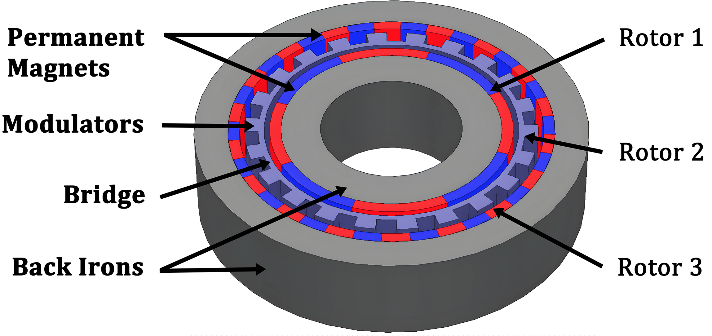
Figure 1: Coaxial radial flux magnetic gear with surface-mounted PMs

Despite advancements, RFMGs face challenges in competing with mechanical counterparts in terms of size, weight, and cost [21]. To fully achieve the potential of MGs, accurate and effective analysis tools are required. Finite element analysis (FEA) is the tool that is most often used, due to its accuracy, accessibility, and robustness in capturing complex nonlinear effects. However, FEA has high computational costs, especially in intricate designs, which can increase the simulation run times [22]. In contrast, analytical models and winding function theory (WFT) offer faster computations but may lack design flexibility and accuracy, particularly in representing complex flux paths and nonlinearities [23, 24]. However, high-resolution magnetic equivalent circuit (MEC) models, which are sometimes referred to as reluctance networks, strike a balance between accuracy and computational efficiency, making them suitable for optimization studies[25, 22].

Previously, [25, 26] introduced a parametrized high-resolution MEC for simplistic RFMGs that accurately tracked design trends. However, it did not account for nonlinearity and became less accurate when ferromagnetic components became thin and saturated[26]. Additionally, it is critical to account for nonlinearity when evaluating RFMGs with bridges between modulators. The bridge is often used to provide structural support and simplify manufacturing for the modulators, which need support against strong magnetic forces due to their position between two sets of PMs. The bridge provides some of this support and simplifies manufacturing but provides a flux leakage path, reducing the slip torque[27, 28, 3]. A relatively thin bridge can also reduce the PM eddy current loss and slightly improve the efficiency relative to designs with no bridge or a thicker bridge[29, 27]. However, the bridge may experience significant saturation that requires a nonlinear model for accurate representation. As an example, Fig. 2 illustrates a 2D design with bridges experiencing saturation. For this design, linear and nonlinear FEA predict slip torques of 1.2 kNm and 6.7 kNm, respectively, which is an 82% discrepancy. The significant disparity between the two results underscores the importance of modeling the nonlinearity. While some previous papers have proposed nonlinear MECs for MGs [30, 31, 32], these papers have failed to demonstrate that their meshes and convergence criteria work consistently across a wide range of designs. Therefore, this paper presents a highly parameterized MEC model and a convergence criterion and evaluates their effectiveness across a wide range of designs.

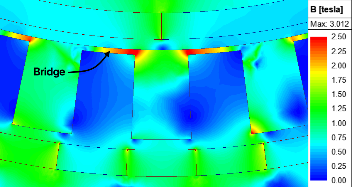
Figure 2: Flux density (B) based on nonlinear FEA in a sample RFMG with bridges

II Implementation

II-A Meshing and the Node Cell

By discretizing (meshing) the MG into radial and angular (tangential) layers, the systematic, parameterized 2D MEC implemented in [25] and [26] is utilized. Fig. 3 shows an example of a source-free MEC, which consists of 3 radial layers, and 12 tangential layers. The boundaries of these layers are denoted by the dotted lines. The overlap of each radial layer with each angular layer defines an arc-shaped region called a 2D node cell. As depicted in Fig. 3 each 2D node cell has four reluctances, two oriented radially and two oriented tangentially. These reluctances represent flux tubes that connect each boundary of the node cell to the center of the node cell, allowing positive or negative flux to flow from the center of the node cell to each of its boundaries.

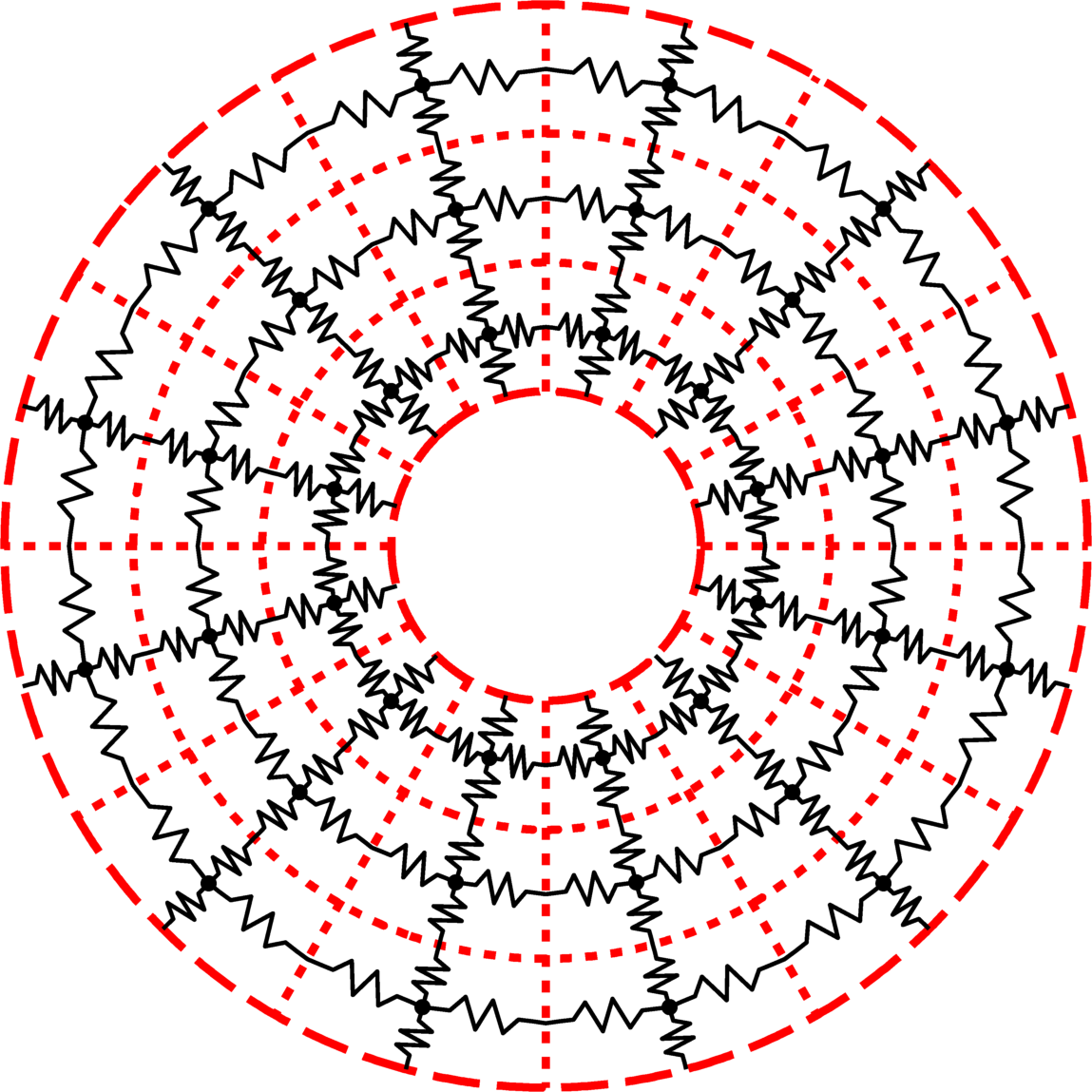
Figure 3: Radial and angular layers and mesh node cells in a simple MEC example

If a flux tube contains a PM magnetized in the direction of the flux tube, an MMF source is placed in series with the reluctance. (In this paper, MMF sources only appear in the flux tubes oriented radially within the PMs since only radially magnetized PMs are considered.) These flux tubes are represented using the equivalent circuit configuration depicted in Fig. 4, in which $\mathcal{R}_{rad}$ denotes the reluctance of the radial flux tube with the permeability of ${\mu}_{PM}$, $\mathcal{F}_{inj}$ signifies the equivalent magnetomotive force (MMF) injected by the PM, $\mathcal{F}_{PM}$ represents the MMF drop across the flux tube, and ${\Phi}_{PM}$ indicates the magnetic flux in the flux tube.

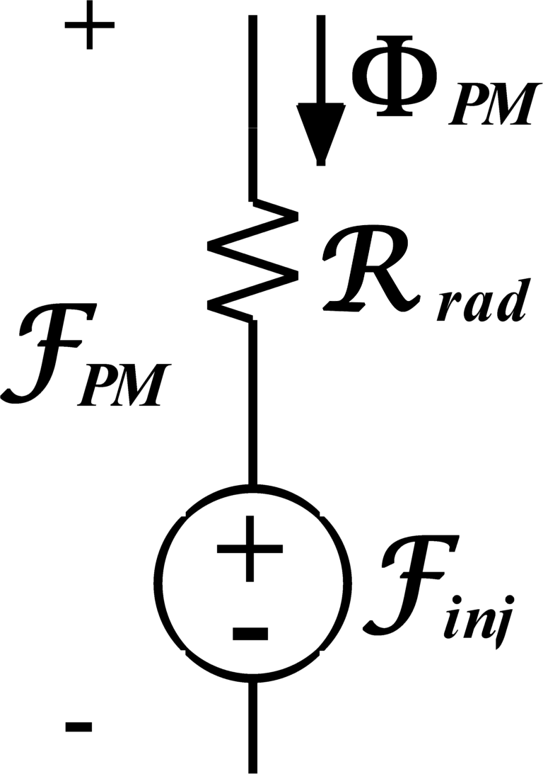
Figure 4: Equivalent circuit representation of a radially oriented permanent magnet flux tube

In this study, as in [25], the MEC mesh is distributed throughout the geometry as illustrated in Fig. 5, depicting a very coarse mesh overlaid on the unrolled representation of an RFMG with $P_{1}=1$, $P_{3}=2$, and $Q_{2}=3$. This mesh distribution divides the geometry into an equal number of angular layers. It partitions the RFMG into eight distinct radial regions, the inner back iron, inner PMs, inner air gap, bridge, modulators, outer air gap, outer PMs, and the outer back iron. The meshing also extends to the air inside the inner back iron and outside the outer back iron. Each of these ten radial regions consists of several radial layers. The user determines the number of radial layers in each region and the number of angular layers based on the tradeoff between analysis speed and accuracy.

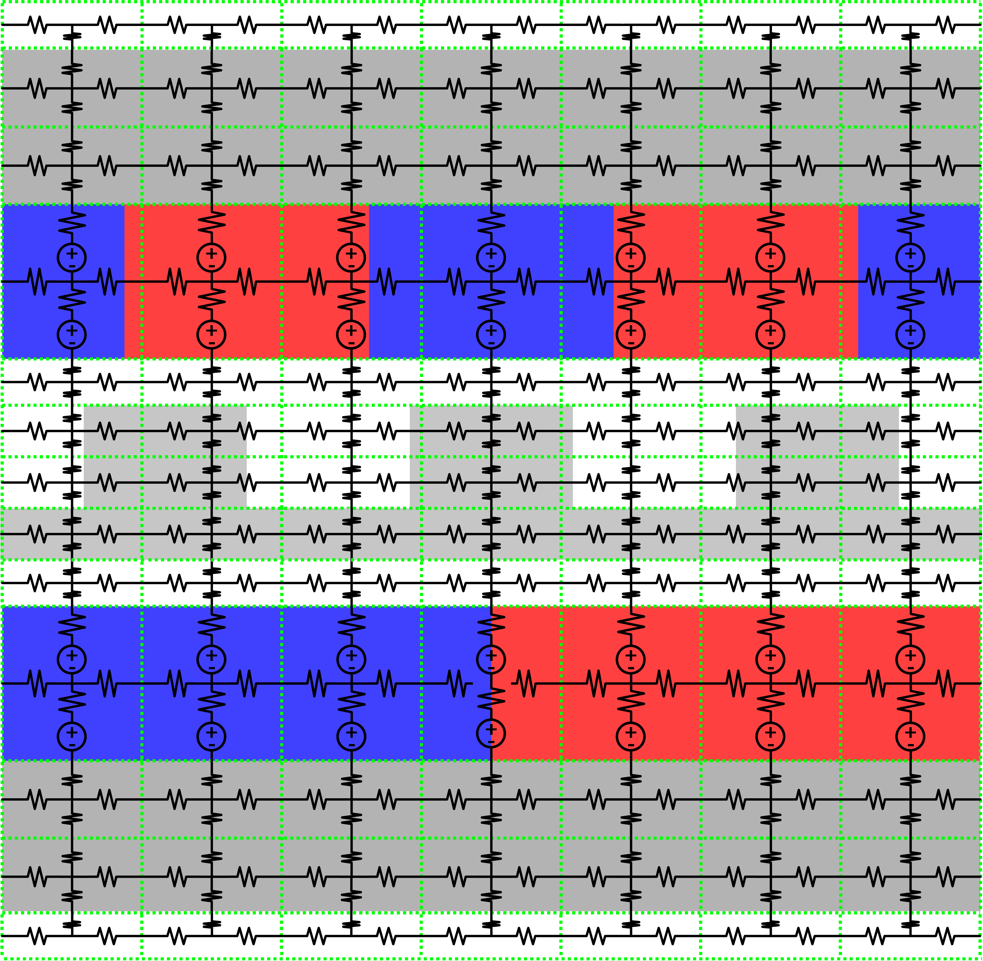
Figure 5: MEC overlaid on an example unrolled RFMG

II-B The System of Nonlinear Equations

The MEC model is developed based on mesh-flux analysis, derived from Ampere’s circuital law, where the circulating magnetic fluxes in each mesh loop represent an independent unknown variable. Mesh-flux analysis is utilized like Kirchhoff’s voltage law is employed in the mesh-current analysis of electrical circuits. As an example, Fig. 6 depicts a mesh loop of the MEC, featuring node cells in the PMs. Loops outside the PMs are modeled similarly, except they lack the MMF sources. Applying Ampere’s law to the mesh loop in Fig. 6, results in a mesh-flux equation of the form

$$\sum_{i=1}^{4}{\mathcal{R}}_{i}(\Phi)({\Phi}_{x}-{\Phi}_{i})=f_{inj,4}-f_{inj,2}$$ (3)

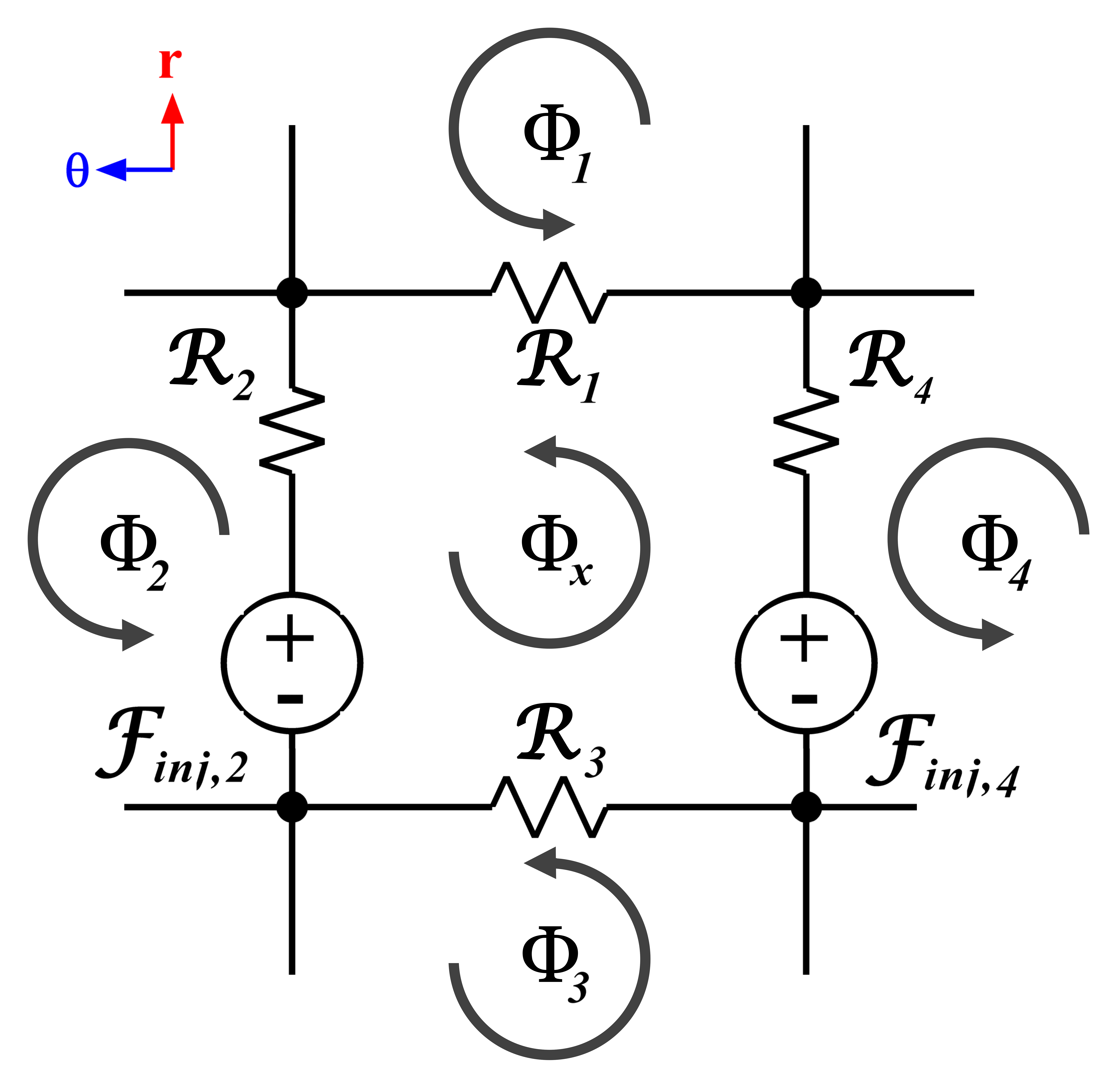
Figure 6: 2D mesh loop schematic

where the left-hand term represents the sum of the reluctances within the mesh multiplied by their respective fluxes. This term characterizes the MMF drop attributed to the reluctances in the loop and equals the sum of the injected MMF sources in that loop. In mesh-flux analysis, reluctances are utilized instead of permeances for ease of calculation. The reluctance of each flux tube is computed similarly to [25], except that, to represent saturation in ferromagnetic materials, the permeability depends on the flux density within the node cell.

The system of nonlinear equations describing the 2D MEC model is achieved by representing every mesh loop in the MEC by a mesh flux equation of the same basic form shown in (3). If the MEC consists of $N_{AL}$ number of angular layers and $N_{RL}$ number of radial layers, the number of mesh loops $N$ equals $N_{AL}\times(N_{RL}-1)$. This MEC model can be expressed in the matrix form as

$$[\mathcal{R}(\Phi)]_{N\times N}[\Phi]_{N\times 1}=[f]_{N\times 1}$$ (4)

where $\mathcal{R}$ is the reluctance matrix, $\Phi$ is the column vector of unknown mesh fluxes, and $f$ is the column vector of the algebraic sum of the MMFs injected by PMs in each loop.

In the reluctance matrix, $\mathcal{R}$, the $i^{th}$ row corresponds to the $i^{th}$ mesh loop in the MEC and contains the reluctance coefficients for that loop’s flux equation, such as those shown on the left side of (3). The $j^{th}$ column in $\mathcal{R}$ corresponds to the $j^{th}$ loop flux in the MEC. Entry $\mathcal{R}_{(i,j)}$ in $\mathcal{R}$ contains the reluctance coefficient which describes the impact of the $j^{th}$ loop’s flux on the net MMF drop around the $i^{th}$ loop. Each diagonal entry $\mathcal{R}_{(i,i)}$ in $\mathcal{R}$ contains the positive sum of all reluctances surrounding the $i^{th}$ loop. The reluctance coefficient of $\Phi_{x}$ in (3) illustrates a diagonal entry within the matrix representation of the system of equations, indicating the impact of the corresponding loop’s flux on the net MMF drop around the loop. Each off-diagonal entry $\mathcal{R}_{(i,j)}$ (where $i\neq j$) in $\mathcal{R}$ contains the negative value of the reluctance through which both the $i^{th}$ and $j^{th}$ loop fluxes pass. If those loops are not adjacent, the corresponding entry in $\mathcal{R}$ is zero. The reluctance coefficients $\mathcal{R}_{1}$, $\mathcal{R}_{2}$, $\mathcal{R}_{3}$, and $\mathcal{R}_{4}$ in (3) exemplify off-diagonal entries in the matrix form of the system of equations. Since all the reluctances in the MEC are bidirectional, the matrix $\mathcal{R}$ is always symmetric. Also, each loop in the MEC has four adjacent loops, except for the innermost and outermost loops, which lack adjacent loops on their radial inside and outside, respectively. As a result, all the rows in $\mathcal{R}$ have five non-zero entries: one for each adjacent loop, as well as the diagonal entry in that row, except for the rows corresponding to the innermost and outermost loops, which have four non-zero entries. If the model exhibits symmetry, the analysis can be simplified by solving only the subset of equations corresponding to the mesh loops within a symmetrical fraction of the model.

Mesh-flux analysis was chosen over the node-MMF analysis used in [25, 26] due to a convergence issue encountered when solving the system of nonlinear equations with the Newton-Raphson method. Mesh-flux analysis directly outputs flux, from which flux density can easily be calculated to update permeability. On the other hand, node-MMF analysis calculates MMF; then, the reluctances, which depend on flux density, must be used to determine magnetic flux. However, this requires the use of reluctances from the previous iteration and can prevent convergence in many cases.

II-C Nonlinear Analysis with Newton-Raphson Method

The 2D MEC model is analyzed by solving the following system of nonlinear equations, which can be rewritten from (4) as

$$\mathcal{R}(\Phi)\times{\Phi}-f=0$$ (5)

This nonlinear equation is solved iteratively using the Newton-Raphson method, as it generally offers relatively fast convergence[33]. Substituting the calculated $\Phi$ for the $k^{th}$ iteration back into the left-hand side of (5) and updating the reluctances in $\mathcal{R}$ yields the residual matrix, $r(\Phi)$, as in

$$\mathcal{R}(\Phi_{k})\times{\Phi_{k}}-f=r(\Phi_{k})$$ (6)

where the goal of the Newton-Raphson method is to find $\Phi_{k}$ such that the residual becomes a column vector of zeros.

To apply the Newton-Raphson method to (6), the following equation is iteratively used to solve for $\Phi$, the root of the equation:

$$\Phi_{k+1}={\Phi}_{k}-\frac{r{(\Phi_{k})}}{r^{\prime}(\Phi_{k})}$$ (7)

Here, $r^{\prime}(\Phi)$ is the Jacobian of $r(\Phi)$, which contains the partial derivatives of this multivariate function with respect to the mesh fluxes. The Jacobian matrix elements are calculated similarly to the reluctance matrix, $\mathcal{R}(\Phi)$, but using differential permeability instead of apparent permeability [34]. Therefore, (7) can be rewritten as

$$\Phi_{k+1}=\Phi_{k}-\frac{\mathcal{R}_{App}(\Phi_{k})\times{\Phi_{k}}-f}{\mathcal{R}_{Diff}(\Phi_{k})}$$ (8)

where $\mathcal{R}_{App}(\Phi_{k})$ and $\mathcal{R}_{Diff}(\Phi_{k})$ represent the reluctance matrix calculated using the apparent and differential permeabilities, respectively.

As a close initial guess for the mesh fluxes improves the robustness and convergence speed for the solver [33], (4) is solved linearly using constant permeabilities to provide the initial guess to begin the Newton-Raphson method. After each iteration, the calculated mesh fluxes are used to compute flux density within each flux tube, which is then utilized to calculate the torque using Maxwell’s stress tensor [25]. The flux densities are also used to update the apparent and differential permeabilities of each ferromagnetic node cell based on the B-H curve. The new permeabilities are used to recalculate $\mathcal{R}_{App}$ and $\mathcal{R}_{Diff}$ for the next iteration of (8). Moreover, matrix factorization is utilized instead of direct inversion in (8) to enhance computational efficiency, numerical stability, and memory usage [35].

III Evaluation

The performance of the MEC model is evaluated by studying the convergence criteria and comparing the torque and flux density predictions with the results from nonlinear FEA models developed in ANSYS Maxwell. First, three diverse magnetic gear base designs, presented in Table I and Fig. 7, were used for initial analyses. Additionally, an extensive parametric design optimization study investigated the MEC’s capability to analyze and optimize a broad spectrum of design variations in comparison with FEA. These designs, along with the base designs, have the same geometries as those presented in [26] except that they have bridges. (As shown in Fig. 2, these bridges saturate heavily and require nonlinear analysis for accurate torque predictions.) The designs use M250 electrical steel for the ferromagnetic components and NdFeB N42 for the PMs. Lastly, the effectiveness of the nonlinear analysis tool in practical applications was validated by developing a MEC model for the prototype from [27].

TABLE I: Magnetic gear base designs specifications

Parameter	Description	Base	Base	Base	Units
		Design 1	Design 2	Design 3
$P_{1}$	Rotor 1 pole pairs	11	4	6
$P_{3}$	Rotor 3 pole pairs	45	34	98
$r_{o}$	Active outer radius	150	175	200	mm
$T_{BI1}$	Rotor 1 back iron thickness	20	35	40	mm
$T_{PM1}$	Rotor 1 PM thickness	9	5	13	mm
$T_{AG1}$	Inner air gap thickness	.5	2	1	mm
$T_{Mods}$	Rotor 2 thickness	11	17	14	mm
$T_{Brg}$	Bridge thickness	.5	1	1.5	mm
$T_{AG2}$	Outer air gap thickness	.5	2	1	mm
$T_{PM3}$	Rotor 3 PM thickness	7	5	7	mm
$T_{BI3}$	Rotor 3 back iron thickness	20	30	25	mm

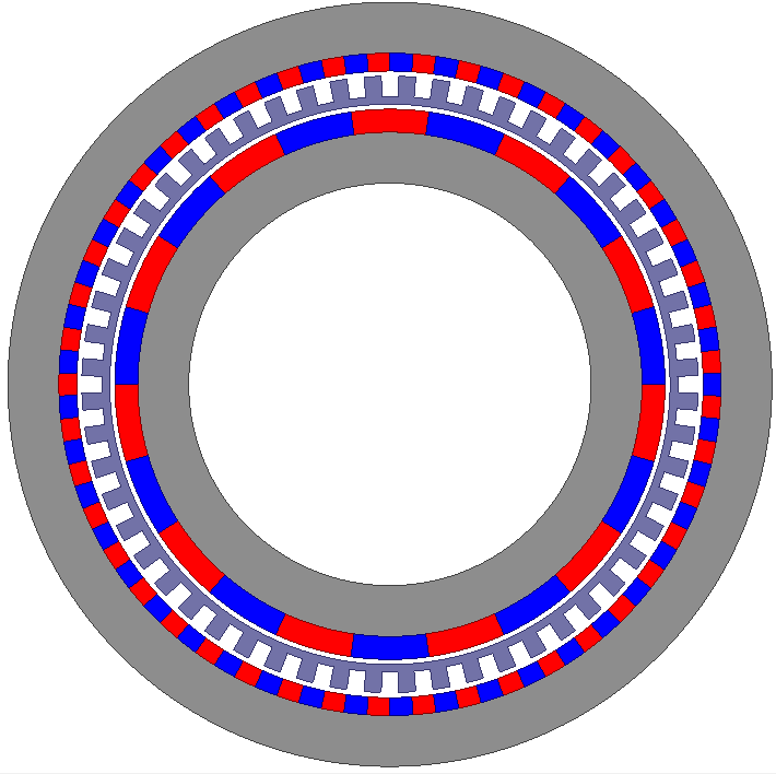
(a)

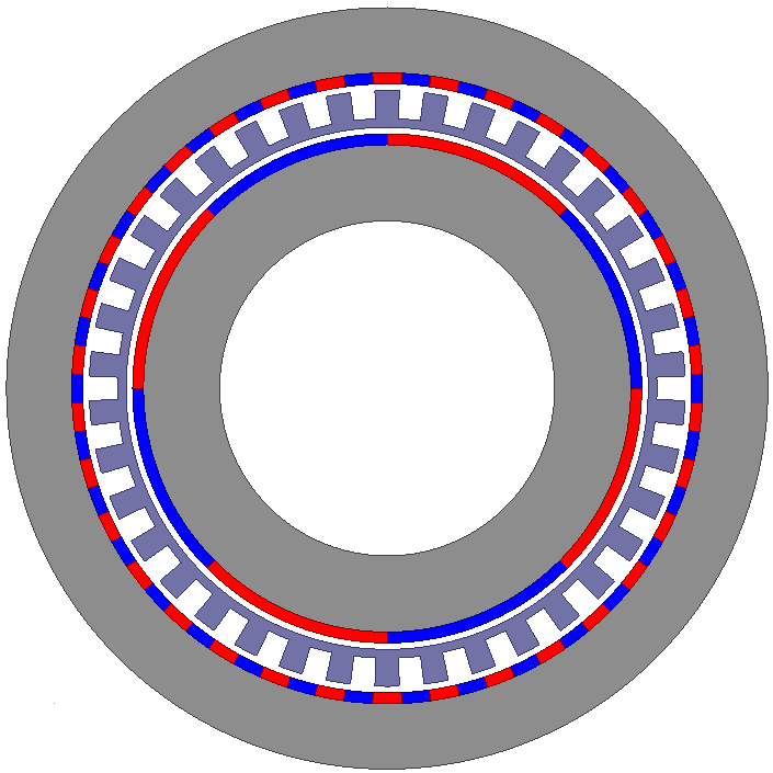
(b)

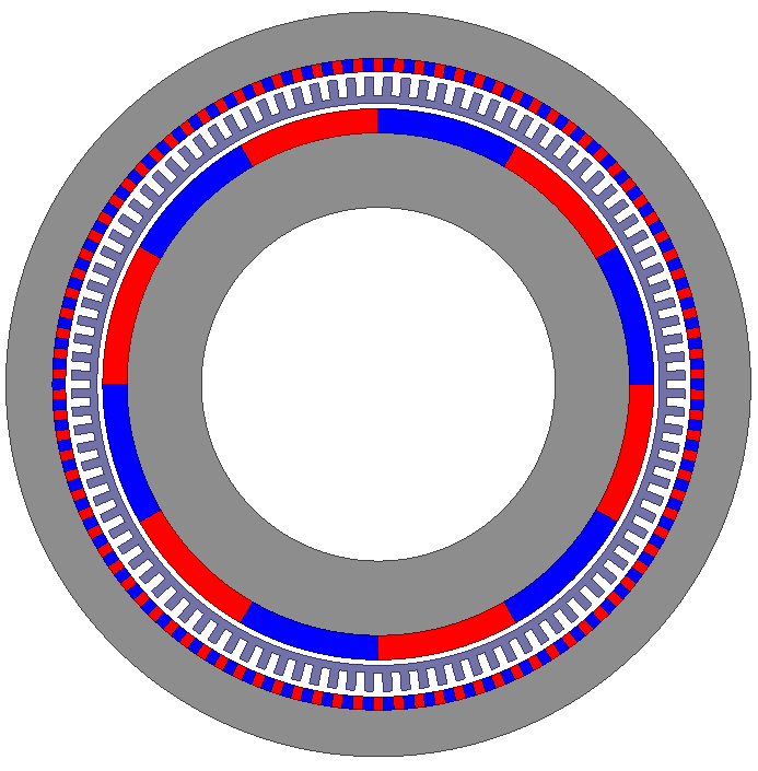
(c)

Figure 7: Cross-sectional views of base designs (a) 1, (b) 2, and (c) 3. (Airgaps and bridges are enlarged for clarity.)

III-A Convergence Criteria

For the optimization of MGs, the torque is a critical performance indicator. Therefore, for this study, an analysis is considered converged when the predicted torque changes less than 0.1% between consecutive iterations. This threshold could be adjusted to trade off precision and speed. Fig. 8(a) depicts the predicted torque after each iteration for three base designs each normalized by the torque after 10 iterations. For all three base designs, the predicted torque quickly converges. Moreover, during convergence, the elements in $r(\Phi)$ should approach zero, which makes the RMS of the residual (depicted in Fig 8(b)) an alternative indicator of the overall solution error. In addition to the torque convergence constraint, we also imposed a constraint that the RMS of the residual must decrease between the final two iterations for the analysis to be considered converged. Fig. 8(c) illustrates the total simulation time after each iteration for each of the base designs. The red circles indicate the iteration in which the torque convergence criteria were achieved. Each base design used the fine mesh discretization parameters from [26] to determine the number of radial and angular layers.

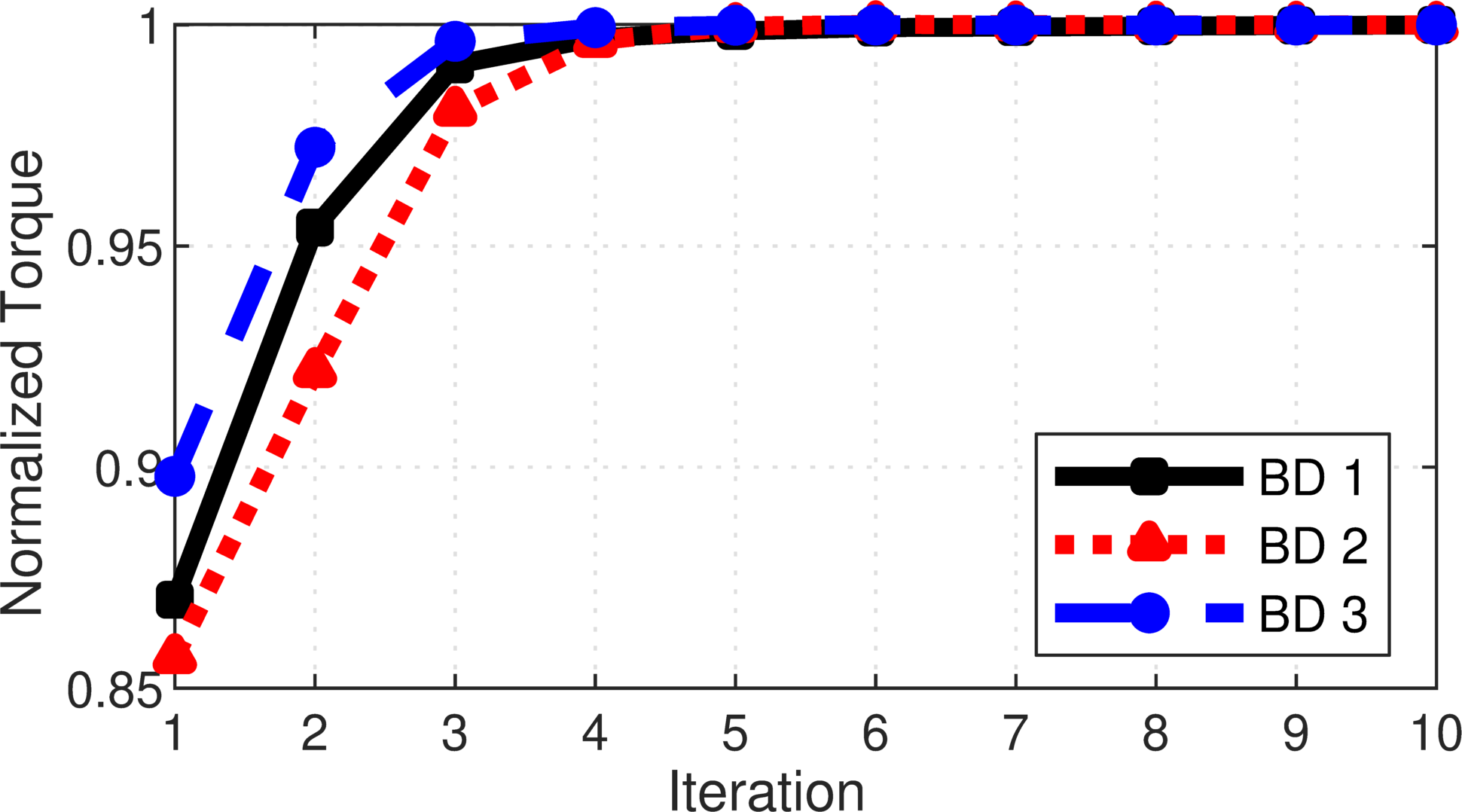
(a)

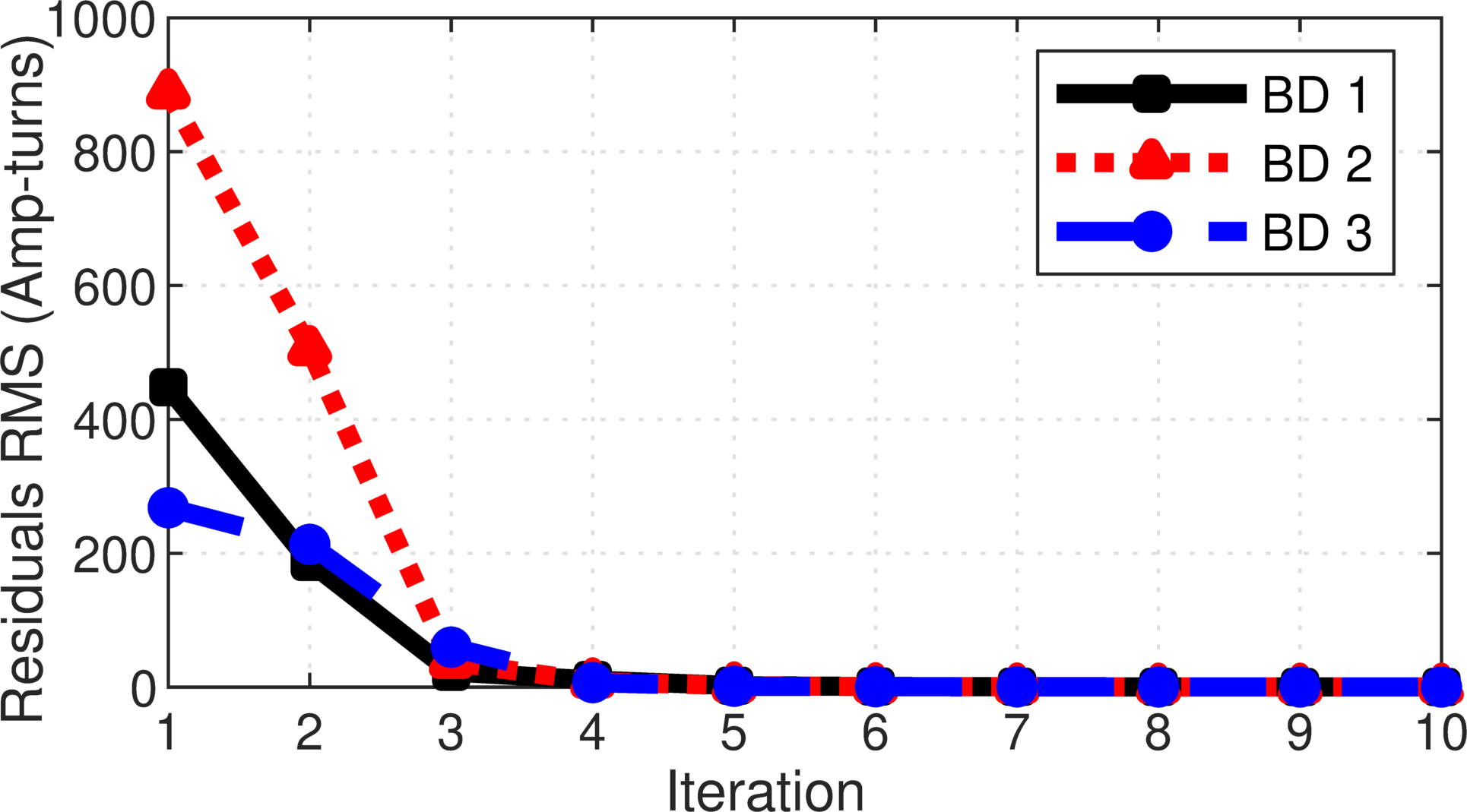
(b)

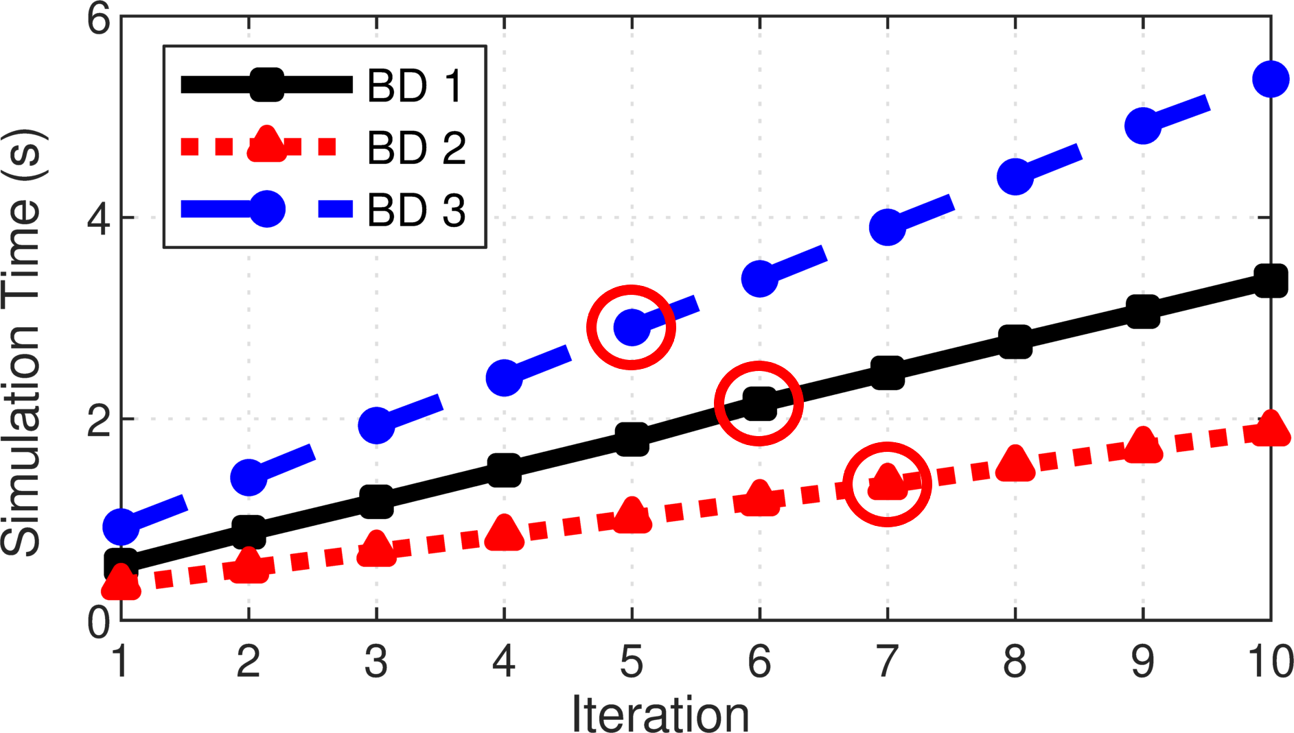
(c)

Figure 8: For each of the base designs, (a) normalized torque, (b) RMS of the residual, and (c) total simulation time for different numbers of iterations

III-B Flux Density Comparisons

The radial flux density distributions shown in Fig. 9 were calculated by the nonlinear FEA and MEC models along circular paths in the middle of the outer air gaps of the three base designs. The results indicate that the MEC produces highly accurate flux density distributions for these three designs.

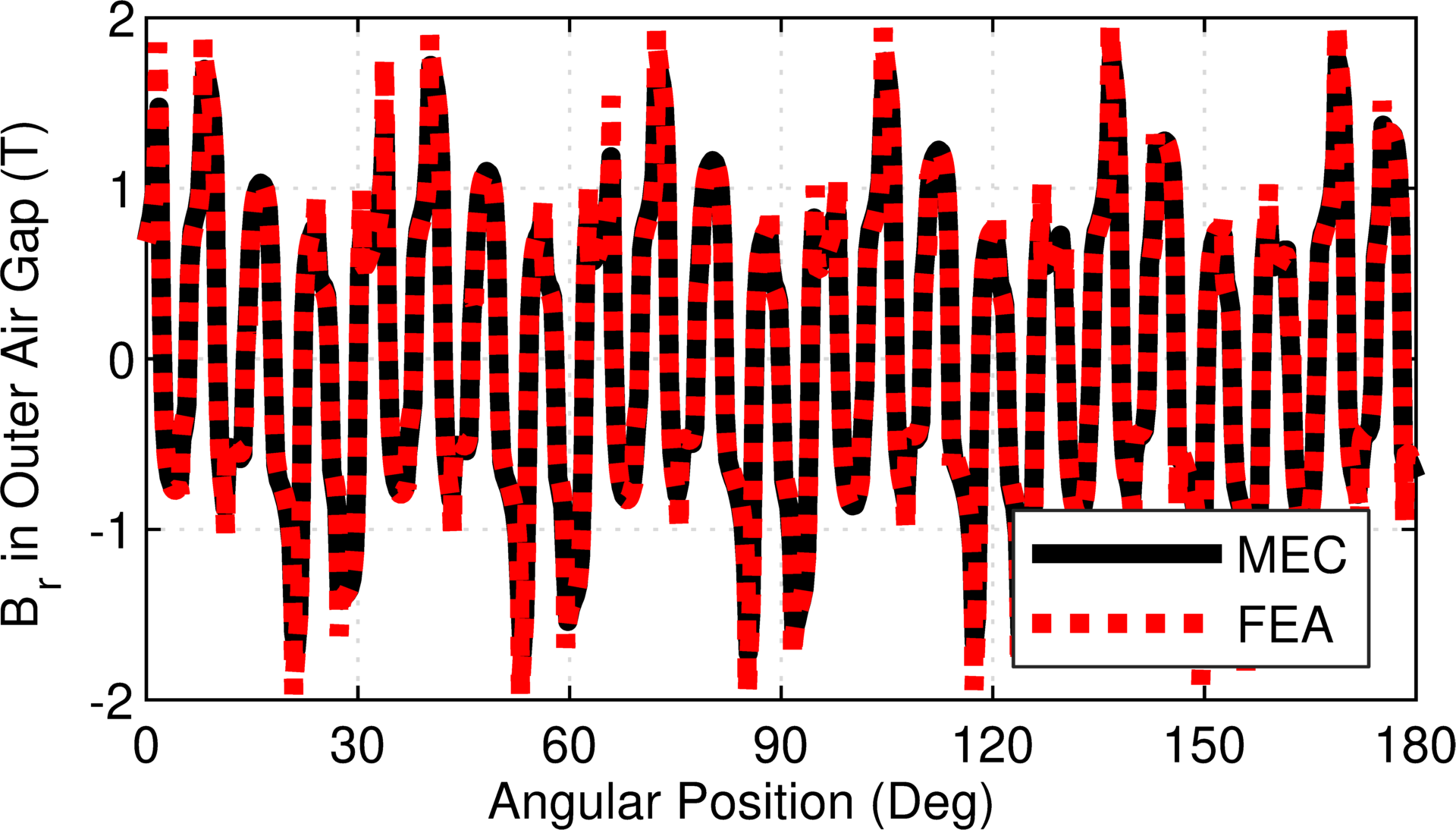
(a)

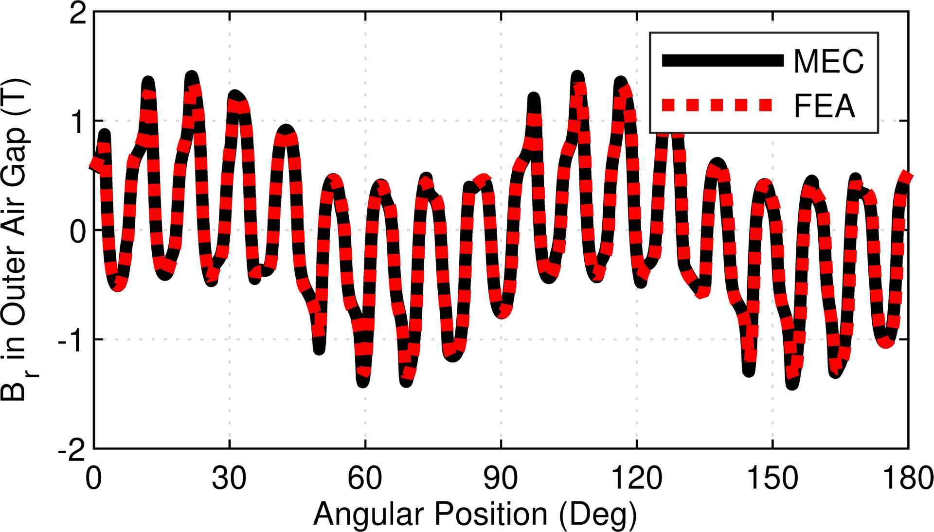
(b)

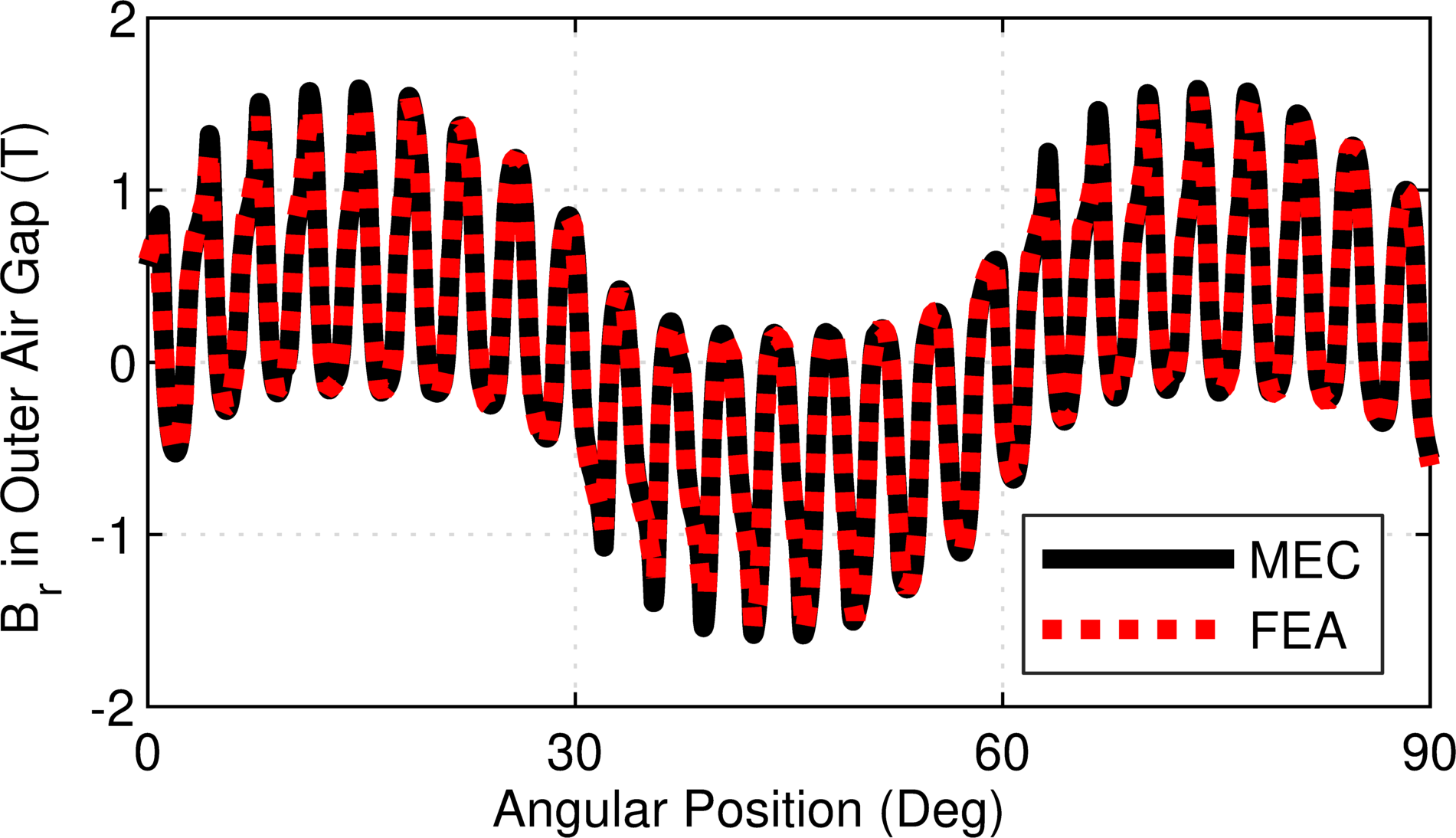
(c)

Figure 9: Radial flux density along a circular path in the middle of the outer air gap of base designs (a) 1, (b) 2, and (c) 3.

III-C Optimization Study

As demonstrated in [26], insufficient radial and angular layer counts can result in fast models with inaccurate slip torque predictions. Similarly, it is important to assess whether the convergence criteria are effective over a wide range of designs. Therefore, a parametric optimization study of RFMGs with bridges was conducted to evaluate the nonlinear MEC as a rapid design tool. To do so, several critical gear parameters were swept over the ranges of values specified in Table II, and each of the resulting 140,000 designs was analyzed using the 2D nonlinear MEC model as well as a 2D nonlinear FEA model developed in ANSYS Maxwell, a commercial FEA software. The MEC analysis was done using two different meshing resolutions, specified as the “coarse mesh” and “fine mesh” settings defined in [26]. Additionally, both coarse and fine mesh settings use two radial layers in the air regions inside the inner back iron and outside the outer back iron, where flux densities are expected to be relatively small. The bridge, being relatively thin, is also divided into only two radial layers.

TABLE II: Parameter sweep ranges for optimization study

Parameter	Description	Ranges	Units
		of Values
$G_{r}$	Integer part of gear ratio	5,9,17
$P_{1}$	Inner pole pairs
	For $G_{r}$ = 5	4,5,6,…18
	For $G_{r}$ = 9	3,4,5,…13
	For $G_{r}$ = 17	3,4,5,…8
$r_{O}$	Active outer radius	150, 175, 200	mm
$k_{BI1}$	Rotor 1 back iron thickness coefficient	0.4, 0.5, 0.6
$T_{PM1}$	Rotor 1 PM thickness	3,5,7,…13	mm
$T_{AG}$	Common air gap thickness	1.5	mm
$T_{Mods}$	Rotor 2 thickness	11, 14, 17	mm
$T_{Brg}$	Bridge thickness	0.5, 1 ,1.5	mm
$k_{PM}$	Rotor 3 PM thickness ratio	0.5, 0.75, 1
$T_{BI3}$	Rotor 3 back iron thickness	20, 25, 30	mm

As in [26], to reflect the significant interactions between the various dimensions, some were coupled through derived coefficients included in Table II. The coefficient $k_{PM}$ relates the radial thickness of the Rotor 3 PMs, $T_{PM3}$, to that of the Rotor 1 PMs, $T_{PM1}$, as expressed by

$$T_{PM3}=k_{PM}\times T_{PM1}$$ (9)

This approach is used because Rotor 3 has a higher PM pole count than Rotor 1, which results in increased flux leakage. Thus, the Rotor 3 PMs should not be thicker than the Rotor 1 PMs. Additionally, the coefficient, $k_{BI1}$, couples the radial thickness of the Rotor 1 back iron to the Rotor 1 pole arc to prevent excessive saturation, according to

$$T_{BI1}=k_{BI1}\left(\frac{\pi r_{BI1}}{P_{1}}\right)$$ (10)

where $r_{BI1}$ is the outer radius of the Rotor 1 back iron, as in [26]. Furthermore, $G_{r}$ represents the integer part of the gear ratio and relates the pole pair counts according to

$$P_{3}=\left\{\begin{aligned} &(G_{\text{int}}-1)P_{1}+1,&&G_{\text{int}}P_{1}\text{ odd}\\ &(G_{\text{int}}-1)P_{1}+2,&&G_{\text{int}}P_{1}\text{ even}\end{aligned}\right.$$ (11)

This avoids integer gear ratios and designs lacking symmetry, which are prone to large torque ripples[2] and unbalanced magnetic forces on the rotors[36], respectively.

The graphs in Figs. 10-13 and the statistics in Table III compare the optimization study results obtained from the fine and coarse-meshed MEC with those from the FEA.

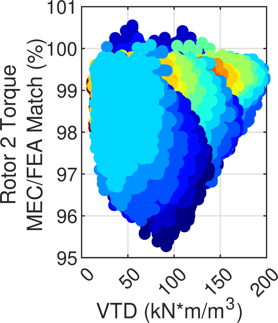
(a)

(b)

Figure 10: MEC agreement with FEA over the full parametric sweep range with the (a) fine mesh and the (b) coarse mesh.

Figure 11: Legend for design trend plots in Figs. 12 and 13

(a)

(b)

Figure 12: Impact of Rotor 1 pole pair count on the maximum achievable (a) VTD and (b) PM VTD.

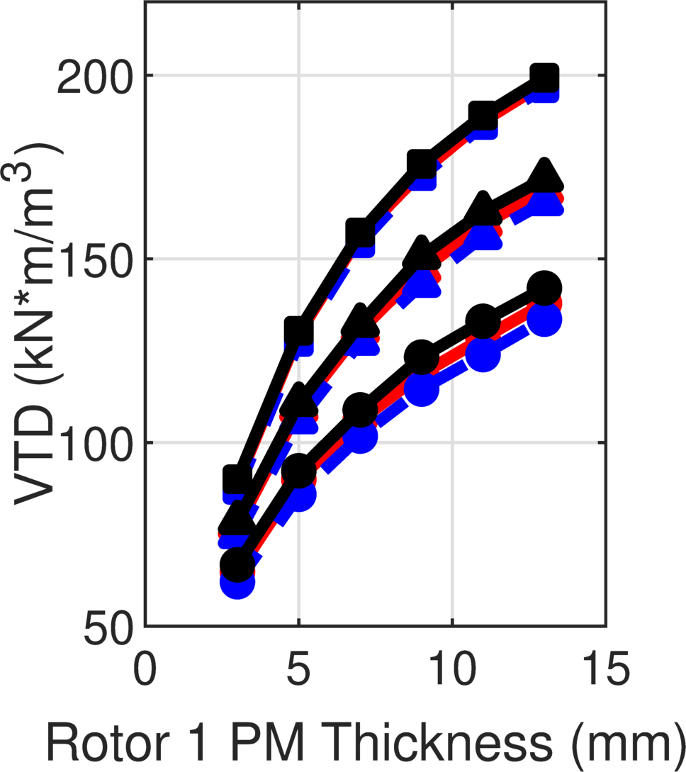
(a)

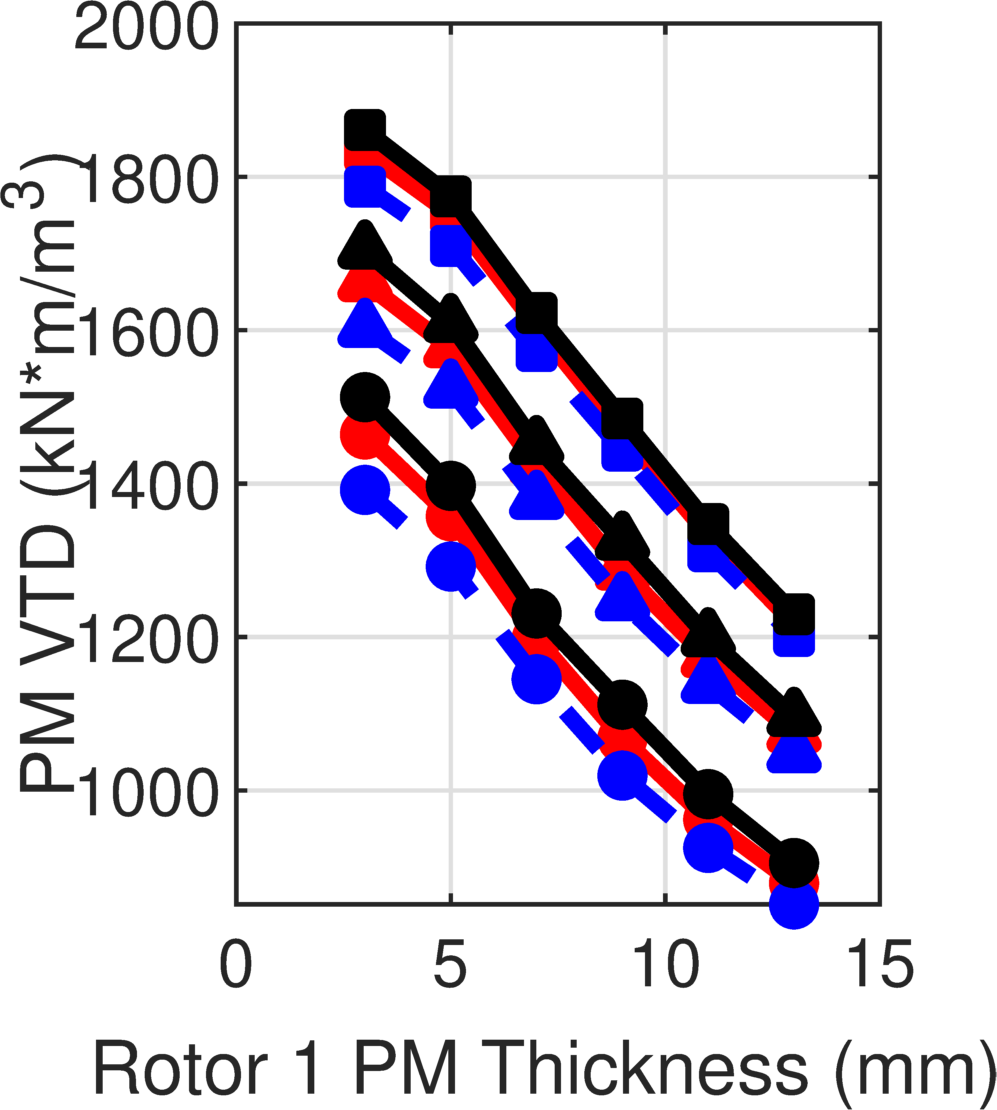
(b)

Figure 13: Impact of Rotor 1 PM thickness on the maximum achievable (a) VTD and (b) PM VTD.

TABLE III: Summary of optimization study results

Metric	Fine Mesh	Coarse Mesh	FEA
	MEC	MEC
Minimum Discrepancy	-4.7%	-9.45%	N/A
Maximum Discrepancy	0.55%	-0.29%	N/A
Average Discrepancy	1.54%	4.33%	N/A
Average Absolute Discrepancy	1.54%	4.33%	N/A
Total Simulation Time (sec)	387,500	60,822	6,003,857
Average Simulation Time (sec)	2.77	0.43	42.89

Fig. 10 demonstrates the accuracy of the MEC models across the entire parametric sweep, indicating their fair accuracy over a wide range of volumetric torque densities (VTDs). Overall, the torque predictions from both fine and coarse mesh MEC models closely correspond to those from FEA models, with discrepancies less than 5% and 10%, respectively. Notably, the MEC models exhibit closer agreement with the FEA for designs with higher VTDs, indicating that the accuracy is best for the designs most likely to be of interest. Specifically, for the designs with the top 10% of VTDs, the maximum absolute discrepancies are 2% and 4.5% for fine and coarse mesh MEC models, respectively. Figs. 12 and 13 indicate the MEC model’s accurate tracking of key performance trends, particularly in VTD and PM VTD (defined as slip torque divided by PM material volume) relative to the Rotor 1 pole pair count and PM thickness. Table III presents a statistical analysis demonstrating the accuracy and speed of the coarse and fine mesh MEC models compared to the FEA model across the entire parametric design space outlined in Table II. On average, the fine and coarse mesh MEC models are about 15 and 100 times as fast as the FEA, respectively.

III-D Prototype Comparison

The nonlinear MEC is also utilized to analyze the magnetic gear portion of the prototype presented in [27] (Fig. 14). To leverage the systematic, parameterized nonlinear MEC model described previously, the prototype is first discretized with the fine mesh setting. The MEC model employs an approximate representation of the RFMG prototype, as depicted in on the right side of Fig. 14, to be consistent with the MEC model used for the optimization study. The rectangular magnets are approximated as arc-shaped. Moreover, each node cell in Rotor 2 is assumed to be wholly one single material, depending on the material constituting the majority of that node cell. This yields the rough modulator surfaces in the approximate design shown in Fig. 14. The small nubs for positioning the PMs are also ignored.

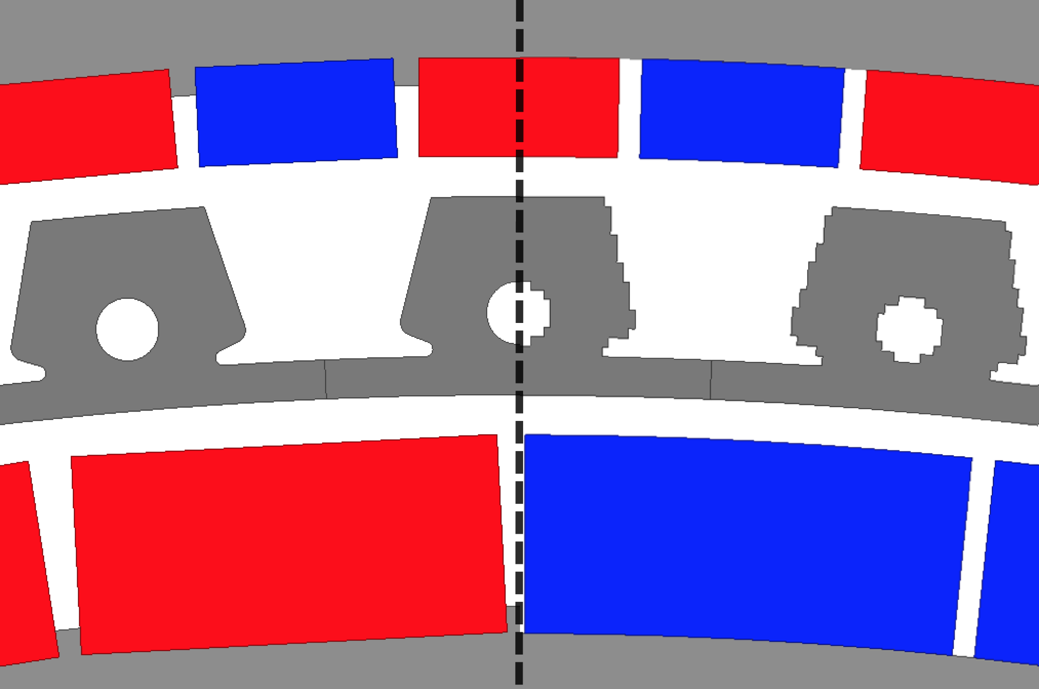
Figure 14: Left: Close-up view of the magnetic gear section in the experimental prototype in [27]. Right: Corresponding approximation used by the MEC model.

Analyzing the approximate design with the MEC yields a Rotor 3 torque of 5.00 kNm, whereas 2D FEA predicts 4.82 kNm based on the original design on the left side of Fig. 14. The discrepancy between 2D FEA and MEC is only 3.7% which shows the close agreement between the two methods. However, the measured torque of 3.87 kNm is significantly lower than the torque predicted by either 2D model. This much larger discrepancy with the experimental measurement results from 3D end effects [27, 37]. Thus, using 3D FEA results in a torque prediction of 3.91 kNm, showing only a 1.0% error compared to the measured torque, which is much smaller than the error from 2D FEA. Therefore, it can be concluded that the 2D nonlinear MEC is about as effective as the 2D FEA, which is commonly used for initial analysis and optimization [38, 39]. Nonetheless, a 3D model is required to accurately predict the torque of RFMGs, making the development of a 3D nonlinear MEC an opportunity for valuable future work.

IV Conclusion

This study presents a fast and robust 2D nonlinear MEC model for radial flux magnetic gears. First, the systematic implementation and analysis of the MEC model are presented. Then, the model is shown to quickly and accurately predict torque and air gap flux densities for a wide range of designs. The modeling begins with discretizing the RFMG into mesh loops, with the meshing resolution of user choice. The system of equations is built by applying mesh-flux analysis on each mesh loop and constructing the reluctance matrix of the RFMG. The resulting system of equations is nonlinear since the reluctance matrix is a function of mesh fluxes. To solve the nonlinear system, Newton-Raphson, an iterative method, is shown to be a fast and reliable approach. The combination of requiring the RMS of the residual to decrease between the last two iterations and requiring the torque variation between the last two iterations to be less than 0.1% proves to be an effective convergence criterion. For three diverse base designs with bridges, the nonlinear MEC agrees very well with FEA on the air gap flux densities. A parametric optimization study with 140,000 designs shows that the nonlinear MEC consistently agrees with FEA on torque predictions and accurately tracks design trends. The results demonstrate that the presented model is able to achieve 15 to 100 times faster analysis while maintaining an average discrepancy of 1.54% and 4.53% relative to the FEA model’s torque predictions for the fine and coarse meshed MECs, respectively. Further assessment and verification are done by comparing the torque prediction to the measured torque of a prototype. The torque prediction using 2D MEC model was first compared to 2D FEA for the prototype and was shown to agree within 3.7%, despite minor approximations to make the geometry conform to the MEC’s grid of node cells. However, there was a 29.2% discrepancy between the MEC and the experimental results, largely resulting from 3D end effects. Thus, the 2D nonlinear MEC presented in this paper, like 2D FEA, may be well suited for initial optimization, but developing a 3D nonlinear MEC that is consistently accurate for diverse RFMG designs would be valuable future work for predicting the torque of prototypes.

Danial Kazemikia earned his B.Sc. degree in electrical engineering from K. N. Toosi University, Tehran, Iran in 2019. He is currently a Ph.D. student in electrical engineering at the University of Texas at Dallas. His research interests are computational electromagnetics, design optimization, and physics-informed neural networks focusing on the design and control of electric machines and magnetic gears.

Matthew C. Gardner earned his B.S. in electrical engineering from Baylor University, Waco, Texas in 2014. He earned his Ph.D. in electrical engineering from Texas A&M University, College Station, Texas in 2019. In August 2020, he joined the University of Texas at Dallas, where he is an assistant professor. His research interests include optimal design and control of electric machines and magnetic gears.

References

- [1] G. Tao et al., “Experimental comparison of acoustic characteristics for a high-efficiency magnetic gearbox and a mechanical planetary gearbox for industrial hvac applications,” IEEE Trans. Energy Convers., vol. 39, no. 1, pp. 182–190, 2024.
- [2] N. W. Frank and H. A. Toliyat, “Gearing ratios of a magnetic gear for wind turbines,” in IEEE Int. Electr. Mach. Drives Conf., 2009, pp. 1224–1230.
- [3] K. Li et al., “Designing and experimentally testing a magnetic gearbox for a wind turbine demonstrator,” IEEE Trans. Ind. Appl., vol. 55, pp. 3522–3533, July 2019.
- [4] A. B. Kjaer, S. Korsgaard, S. S. Nielsen, L. Demsa, and P. O. Rasmussen, “Design, fabrication, test, and benchmark of a magnetically geared permanent magnet generator for wind power generation,” IEEE Trans. Energy Convers., vol. 35, pp. 24–32, Mar. 2020.
- [5] K. K. Uppalapati, J. Z. Bird, D. Jia, J. Garner, and A. Zhou, “Performance of a magnetic gear using ferrite magnets for low speed ocean power generation,” IEEE Energy Convers. Congr. Expo. (ECCE), pp. 3348–3355, 2012.
- [6] P. O. Rasmussen, T. V. Frandsen, K. K. Jensen, and K. Jessen, “Experimental evaluation of a motor-integrated permanent-magnet gear,” IEEE Trans. Ind. Appl., vol. 49, no. 2, pp. 850–859, 2013.
- [7] T. V. Frandsen, P. O. Rasmussen, and K. K. Jensen, “Improved motor integrated permanent magnet gear for traction applications,” in IEEE Energy Convers. Congr. Expo. (ECCE), 2012, pp. 3332–3339.
- [8] T. V. Frandsen et al., “Motor integrated permanent magnet gear in a battery electrical vehicle,” IEEE Trans. Ind. Appl., vol. 51, no. 2, pp. 1516–1525, 2015.
- [9] P. Chmelicek, S. D. Calverley, R. S. Dragan, and K. Atallah, “Dual rotor magnetically geared power split device for hybrid electric vehicles,” IEEE Trans. Ind. Appl., vol. 55, no. 2, pp. 1484–1494, 2019.
- [10] P. O. Rasmussen, H. H. Mortensen, T. N. Matzen, T. M. Jahns, and H. A. Toliyat, “Motor integrated permanent magnet gear with a wide torque-speed range,” in IEEE Energy Convers. Congr. Expo. (ECCE), 2009, pp. 1510–1518.
- [11] T. F. Tallerico, Z. A. Cameron, J. J. Scheidler, and H. Hasseeb, “Outer stator magnetically-geared motors for electrified urban air mobility vehicles,” in AIAA/IEEE Electr. Aircr. Technol. Symp. (EATS), 2020, pp. 1–25.
- [12] R. S. Dragan, R. E. Clark, E. K. Hussain, K. Atallah, and M. Odavic, “Magnetically geared pseudo direct drive for safety critical applications,” IEEE Trans. Ind. Appl., vol. 55, no. 2, pp. 1239–1249, 2019.
- [13] G. Puchhammer, “Magnetic gearing versus conventional gearing in actuators for aerospace applications,” in Aero. Mech. Symp., 2014, pp. 175–181.
- [14] V. M. Asnani, J. J. Scheidler, and T. F. Tallerico, “Magnetic gearing research at nasa,” in AHS Int. Annu. Forum, 2018, pp. 1–14.
- [15] J. J. Scheidler, V. M. Asnani, and T. F. Tallerico, “Nasa’s magnetic gearing research for electrified aircraft propulsion,” in AIAA/IEEE Electr. Aircr. Technol. Symp. (EATS), 2018, pp. 1–12.
- [16] J. J. Scheidler, Z. A. Cameron, and T. F. Tallerico, “Dynamic testing of a high-specific-torque concentric magnetic gear,” in Vertical Flight Soc. Annu. Forum, 2019, pp. 1–8.
- [17] T. F. Tallerico, Z. A. Cameron, J. J. Scheidler, and H. Hasseeb, “Outer stator magnetically-geared motors for electrified urban air mobility vehicles,” in AIAA/IEEE Electr. Aircr. Technol. Symp. (EATS), 2020, pp. 1–25.
- [18] B. Praslicka, M. C. Gardner, M. Johnson, and H. A. Toliyat, “Review and analysis of coaxial magnetic gear pole pair count selection effects,” IEEE J. Emerg. Sel. Top. Power Electron., vol. 10, no. 2, pp. 1813–1822, 2022.
- [19] B. Praslicka et al., “Design and analysis of an axial flux coaxial magnetic gear with balanced axial forces for precision aerospace actuation application,” in IEEE Energy Convers. Congr. Expo. (ECCE), 2022, pp. 1–8.
- [20] H. Y. Wong, H. Baninajar, B. W. Dechant, P. Southwick, and J. Z. Bird, “Experimentally testing a halbach rotor coaxial magnetic gear with 279 nm/l torque density,” IEEE Trans. Energy Convers., vol. 38, no. 1, pp. 507–518, 2023.
- [21] E. Gouda, S. Mezani, L. Baghli, and A. Rezzoug, “Comparative study between mechanical and magnetic planetary gears,” IEEE Trans. Magn., vol. 47, no. 2, pp. 439–450, 2011.
- [22] X. Ran, J. Shang, M. Zhao, and Z. Yi, “Improved configuration proposal for axial reluctance resolver using 3-d magnetic equivalent circuit model and winding function approach,” IEEE Trans. Transp. Electrif., vol. 9, no. 1, pp. 311–321, 2023.
- [23] G. Vidanalage, B. D. Silva, A. Lombardi, J. Tjong, and N. C. Kar, “Magnetic field-based induction machine modeling incorporating space and time harmonic effects,” IEEE Access, vol. 12, pp. 41 579–41 589, 2024.
- [24] P. Wu and Y. Sun, “A hybrid model for calculating on-load performance of delta-type ipm machines accounting for rotor and stator saturation,” IEEE Trans. Ind. Electron., pp. 1–11, 2024.
- [25] M. Johnson, M. C. Gardner, and H. A. Toliyat, “A parameterized linear magnetic equivalent circuit for analysis and design of radial flux magnetic gears—part i: Implementation,” IEEE Trans. Energy Convers., vol. 33, pp. 784–791, June 2018.
- [26] ——, “A parameterized linear magnetic equivalent circuit for analysis and design of radial flux magnetic gears–part ii: Evaluation,” IEEE Trans. Energy Convers., vol. 33, pp. 792–800, June 2018.
- [27] M. Johnson et al., “Design, construction, and analysis of a large-scale inner stator radial flux magnetically geared generator for wave energy conversion,” IEEE Trans. Ind. Appl., vol. 54, no. 4, pp. 3305–3314, 2018.
- [28] H. Baninajar et al., “Designing a halbach rotor magnetic gear for a marine hydrokinetic generator,” IEEE Trans. Ind. Appl., vol. 58, no. 5, pp. 6069–6080, 2022.
- [29] S. A. Khan, G. Duan, and M. C. Gardner, “Comparison of modulator retention shapes for radial flux coaxial magnetic gears,” in IEEE Energy Convers. Congr. Expo. (ECCE), 2022, pp. 1–7.
- [30] H. Diab, Y. Amara, and G. Barakat, “A 3d nonlinear magnetic equivalent circuit model for an axial field flux focusing magnetic gear: Comparison of fixed-point and newton–raphson methods,” Mathematics and Computers in Simulation, 2023.
- [31] M. Fukuoka, K. Nakamura, and O. Ichinokura, “Dynamic analysis of planetary-type magnetic gear based on reluctance network analysis,” IEEE Trans. Magn., vol. 47, no. 10, pp. 2414–2417, 2011.
- [32] R. Benlamine, T. Hamiti, F. Vangraefschepe, F. Dubas, and D. Lhotellier, “Modeling of a coaxial magnetic gear equipped with surface mounted pms using nonlinear adaptive magnetic equivalent circuits,” in IEEE Int. Conf. Elect. Mach., 2016, pp. 1888–1894.
- [33] S. C. Chapra and R. P. Canale, Numerical Methods for Engineers., 7th ed. McGraw Hill, 2015.
- [34] B. Boomiraja and R. Kanagaraj, “Convergence behaviour of newton-raphson method in node- and loop-based non-linear magnetic equivalent circuit analysis,” in IEEE Int. Conf. Power Electron. Smart Grid Renew. Energy (PESGRE), 2020, pp. 1–6.
- [35] T. A. Davis, “Algorithm 930: Factorize: An object-oriented linear system solver for matlab,” ACM Trans. Math. Softw, vol. 39, no. 4, pp. 1–18, Jul. 2013.
- [36] G. Jungmayr, J. Loeffler, B. Winter, F. Jeske, and W. Amrhein, “Magnetic gear: Radial force, cogging torque, skewing and optimization,” in IEEE Energy Convers. Congr. Expo. (ECCE), 2015, pp. 898–905.
- [37] S. Gerber and R-J.Wang, “Analysis of the end-effects in magnetic gears and magnetically geared machines,” in Int. Conf. Electr. Mach. (ICEM), 2014, pp. 396–402.
- [38] S.-H. Lee, S.-Y. Im, J.-Y. Ryu, and M.-S. Lim, “Optimum design process of coaxial magnetic gear using 3d performance prediction method considering axial flux leakage,” IEEE Trans. Ind. Appl., vol. 60, no. 2, pp. 3075–3085, 2024.
- [39] R. Safarpour and S. Pakdelian, “Topology optimization of the reluctance coaxial magnetic gear,” IEEE Trans. Magn., vol. 58, no. 8, pp. 1–7, 2022.