Deep learning of optical spectra of semiconductors and insulators
Abstract
Despite its potential, optical spectrum prediction for crystalline materials has been largely overlooked in machine learning for materials science. Here we present a proof of concept by creating a ab initio database of 9,915 dielectric tensors of semiconductors and insulators calculated in the independent particle approximation, and subsequently training graph attention neural networks to predict the dielectric function and refractive index. Our study shows that accurate prediction of optical spectra is possible using only the crystal structure and a database of about materials.
Introduction.— In recent years, modern machine learning (ML) techniques have been successfully applied to many problems in materials science, ranging from the prediction of various macroscopic properties such as the formation energy [1, 2, 3, 4, 5], the band gap [6, 7, 8, 9, 10, 11, 12, 13, 14], the static dielectric constant [15, 16], the critical temperature of superconductors [17, 18, 19], and many others too numerous to mention here, to the prediction of novel, possibly stable materials [20, 21, 22, 23, 24, 25]. Despite the highlighted rapid progress of ML in materials science, the prediction of optical spectra for crystalline materials remains surprisingly unexplored, while offering the possibility of finding novel or tailored materials for photovoltaic systems [26], photocatalytic water splitting applications [27, 28, 29, 30, 31], epsilon-near-zero materials [32, 33, 34], optical sensors, light-emitting devices and other optical applications. The notable absence of machine-learned optical spectra in the literature is further emphasized by a look at the “Roadmap on Machine learning in electronic structure” [35], where optical spectra, i.e. the dielectric function or the refractive index , are hardly mentioned, and where the section on deep learning (DL) spectroscopy refers mainly to vibrational spectra, which are dominated by nuclear motions, that are comparatively easy to calculate.
The main reason for the low ML effort in optical properties is the unavailability of datasets and the difficulty to generate sufficiently large and robust datasets from experiments or theory, which is a necessary prerequisite for any ML method. To our knowledge, the largest database of calculated optical spectra to date consists of the absorption spectra of 1,116 compounds as part of the Materials Project [36]. For molecular compounds, optical and X-ray spectra are more widely available [37] and have led to encouraging first results regarding the application of ML [38, 39, 40, 41]. However, crystals are a very different subset of the material space and require very different modeling from the perspective of theoretical physics and ML, respectively.
In order to gain insight into whether it is possible to predict frequency-dependent optical spectra of crystalline solids with state-of-the-art DL models, we use ab initio calculations to create a database of the frequency-dependent dielectric tensors for 9,915 crystalline semiconductors and insulators, from which all other linear optical properties can be calculated.
In this letter, we focus on gapped materials, because of the additional complications that arise when calculating the optical spectra of metals: Mainly, metals require extremely dense k-point sampling to accurately resolve intraband and interband transitions around the Fermi energy, requiring either significantly more computational resources or the use of specialized codes [42].
Leveraging our database, we convert all crystal structures to graphs and then train a graph attention neural network built from off-the-shelf parts found in literature on a subset of it and evaluate its performance on a different test subset. The trained network, together with the graph generation algorithm, allows for the evaluation of optical spectra directly from atomic positions in a fraction of the time of expensive ab initio calculations, while still capturing the key physical features and delivering satisfying quantitative accuracy.
Database.— To create the ab initio database necessary for the application of ML techniques, we perform high-throughput calculations of the dielectric function for 9,915 compounds. The structures are taken from the Alexandria database [24] of theoretically stable crystals, filtered by the following criteria: only main-group elements from the first five rows of the periodic table, less than 13 atoms in the unit cell, distance from the convex hull less than 50 meV per atom, indirect band gap greater than 500 meV. The structures are then reduced to their primitive standard structure according to the algorithm used in Refs. [43, 44]. Density functional theory (DFT) calculations were performed with the plane-wave code Quantum ESPRESSO [45, 46] using PBE [47] as exchange-correlation functional and optimized norm-conserving Vanderbilt pseudopotentials from the SG15 library (version 1.2) [48]. Note that our band gaps may differ slightly from those in the Alexandria database, since the Alexandria database was created with the VASP code [49, 50], using different pseudopotentials. Of the 10,189 compounds in the Alexandria database which fulfill the criteria listed above, 274 were identified to be metals when using Quantum ESPRESSO and SG15 pseudopotentials and were therefore excluded.
First, the DFT calculations were converged using the protocol described previously in Refs. [43, 44]. Then the k-point grid was shifted off symmetry and the -component of the dielectric tensor was calculated in the independent particle approximation (IPA) on an energy grid consisting of equally spaced points in the energy range 0 – 20 eV as implemented in Yambo [51, 52]. At this stage, all spectra were calculated with a broadening parameter meV [52]. In the next step, the density of the shifted k-point grid density was iteratively increased until the similarity between the component of was sufficiently high. To quantify the similarity between frequency-dependent properties, we use the similarity coefficient [53], which is defined as follows
| (1) |
where , are the frequency-dependent properties to be compared. For the convergence with respect to , we used a threshold of 0.9 (cf. Ref. [53], where a threshold of 0.75 is used). Using the converged value, final IPA calculations are performed with two broadening values, meV and meV, to investigate the effect of different broadening values on the performance of the ML models. Additionally, if required by the (lack of) symmetry, the and components of the dielectric tensor are also computed for both values of .
Before using the database for ML, we removed a few outliers with indirect gaps (defined as the difference between the valence band minimum and the conductance band maximum, regardless of their position in k-space) above 10 eV, mainly noble gases. Materials with an indirect gap below 500 meV are also removed, as these may be metals where a band crossing may have been missed. After filtering, the final database used for the subsequent ML consists of 9,748 different materials.
Network Architecture and Training.— With the database now available, we, in the framework of DL, attempt to predict the spectra of new materials simply from trends contained in the data set, in a fraction of the time that an ab initio calculation would take. For this purpose, we apply a Graph Neural Network (GNN) [54], which belong to the class of DL algorithms, as they consist of multiple stacked neural network layers. We convert the crystal structures into multi-graphs [8] by creating a node for each atom in the unit cell and creating an edge between nodes if the distance between corresponding atoms is less than 5 Å, taking into account periodic boundary conditions. As initial node embeddings, we use a one-hot encoding of the atom’s group and row in the periodic table. As edge embeddings we use the Gaussian expanded bond distance, i.e., we evaluate for distances between 0 Å and 5 Å using a step size of Å a Gaussian distribution with standard deviation Å and mean , where is the distance between the corresponding atoms. and can be considered as hyperparameters that we did not optimize in this letter. Following the results of Ref. [55], which found only a small improvement in the density of states (DOS) prediction error by using more advanced representations, we simply represent the frequency-dependent optical spectra we are interested in as a -dimensional vector.
The network’s architecture is as follows: First, the node embeddings are passed through a fully connected neural network to learn the embedding and expand the parameter space. Then, the graph attention operator from Ref. [56] is applied in one to three message passing layers to obtain a high-dimensional node embedding, where the number of message-passing layers used is a hyperparameter. These embeddings are then pooled according to the following operation inspired by the graph attention operator:
| (2) |
where is the final learned representation of the graph, is the learned representation of the -th node of the graph, is a learned matrix, is a learned bias vector and the multiplication with is carried out elementwise. The vector is then finally passed through a multilayer perceptron mapping to the -dimensional output vector. We use rectified linear units () as the activation function in all cases.
As noted in Ref. [25], using a simple train-test split on a dataset can result in compounds with the same chemical composition but (sometimes only slightly) different crystal structures being present in both the training and test sets, leading to improved error measures, but not to improved generalization for chemical formulas not present in either set. Therefore, we index all unique compositions in the dataset and randomly select 80% of the compositions for training and 10% each for validation and testing. For example, if the composition Al2O3 were among those selected for training, all polymorphs of Al2O3 would be included in the training set and thus excluded from the test set. Detailed information on the loss function, training process and hyperparameter optimization can be found in the Supplemental Material (SM).
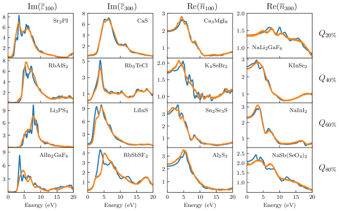
Results.— In this letter, we focus on learning the average of the dielectric function over the diagonal elements of the dielectric tensor, i.e. and the resulting averaged refractive index defined as . For a total of four final models and for both broadening values, meV and meV, we evaluate and as described. In Fig. 1, we show a comparison between the ab initio spectra and the output of the trained models for the 20th, 40th, 60th, and 80th quantile of the test set, as measured by the similarity coefficient . In the SM, we show the same comparisons for a larger, randomly selected subset of the test set. Overall, an extraordinary qualitative and a very good quantitative agreement is found. First of all, the DL model shows no aphysical artifacts such as discontinuities, significant noise or extreme values, even though continuity or smoothness etc. of the predicted spectra were neither enforced nor promoted during DL by, e.g., additional regularizations. A final transposed convolution layer, which would remove such artifacts if they appeared, did not improve the results and does not seem necessary for learning spectral properties.
In general, the structure and scale of the optical spectra obtained through DL are very similar to those from ab initio calculations, especially for compounds with rather simple spectra consisting of only a few strong peaks. In most cases where the intensity of a peak is not predicted well, the position of the peak is still approximately correct. As expected, the model trained on the data calculated with meV broadening shows significantly less structure than the model trained on the data calculated with a meV broadening. Generally, the output of the models shows less structure than the ab initio spectra. This is especially noteworthy for the case of meV broadening, where the spectra of various materials still appear to have significant k-point ripples due to insufficient k-point sampling in the ab initio calculation, which are often difficult to distinguish from actual transitions (see, e.g., Ref. [57] regarding artifacts due to insufficient k-point sampling). Since k-point ripples are essentially an aphysical and hard-to-predict artifact, we interpret this observation as a highly welcome consequence of the fact that the mapping from the “crystal structure to the contribution of k-point ripples” is much harder to learn than the physical mapping from the “crystal structure to the dielectric function”. We note in passing that the challenges of the model in describing highly structured signals can also be observed in the literature on DOS learning [58]. Remarkably, our model is also able to predict the height of the refractive index curve, i.e. the mean refractive index over the frequency range, see Fig. 1.
| MSE | 0.90 (0.30) | 0.44 (0.11) | 0.03 (0.01) | 0.02 (0.01) |
|---|---|---|---|---|
| MAE | 0.38 (0.33) | 0.26 (0.20) | 0.10 (0.09) | 0.08 (0.07) |
| MAPE | - | - | 7.8% (6.7%) | 5.8% (5.0%) |
| 0.78 (0.81) | 0.86 (0.88) | 0.93 (0.94) | 0.94 (0.95) |
We show several quantitative error measures, i.e., the mean square error (MSE), the mean absolute error (MAE), the mean average percentage error (MAPE), and evaluated on the test set for the four models trained in Tab. 1. A recent publication by Carriço et al. [59] predicting the static refractive index, i.e. , using a similar architecture on a different ab initio database, obtained a MAPE on the test set of about 4.5 – 6%, similar to our results.
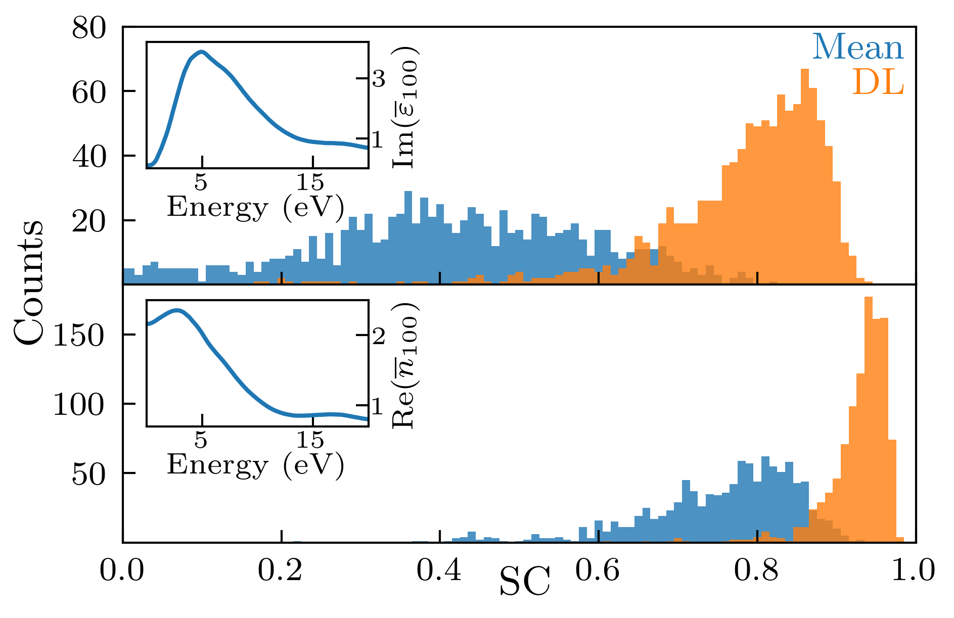
Finally, to gain some insight into the difficulty of the task, we evaluate the obtained by taking the frequency-resolved mean of the training set as a prediction for the and the test sets. This leads to a significantly worse mean (median) similarity coefficient of 0.31 (0.39) and 0.76 (0.78), respectively. Fig. 2 shows the distribution of similarity coefficients between this baseline and the DL model. A dramatically better prediction of the model compared to the mean is evident.
Conclusions.— The results presented in this letter show that DL models commonly used in materials science are able to learn the spectral properties of semiconductors and insulators without significant adaptations to the model architecture and without the need for a much larger database, as might be feared when learning a high-dimensional vectorial quantity instead of a scalar. Significant features are well reproduced. In the case of the refractive index, our frequency-dependent model prediction achieves a quantitative accuracy similar to one recently obtained for the (scalar) static refractive index [59]. As is often the case with machine learning, it is instructive to examine the outliers: the GNN performs especially poorly in predicting the properties of solid fluorine, likely because no other compound contained neutral F atoms. Similarly, planar BN presented challenges.
The most obvious way to improve the current DL model is to increase the size of the dataset used for training, both by including additional elements such as the transition metals or lanthanides (taking into account the challenges of treating them with ab initio methods) to allow the network to generalize to more compounds, and by including more compounds containing the elements already included to improve performance. Another promising direction is that instead of using separate models to learn the real and imaginary parts of or , one could design a model that learns both at the same time, since both parts are connected by the Kramers-Kronig relations. Following the principles of physics-informed neural networks, one could incorporate the Kramers-Kronig relations into the loss functions [58, 60].
One aspect that should be mentioned is the limitation of the underlying ab initio data, which we knowingly accept for this proof-of-concept paper. We neglect local field effects by using the IPA instead of the random phase approximation (RPA) and completely miss excitonic effects, which can be accounted for by the computationally much more demanding Bethe-Salpeter equation (BSE) [61]. Furthermore, the use of Kohn-Sham DFT eigenvalues leads to a general underestimation of band gaps and thus of the absorption edge which can be corrected by a more expensive G0W0 calculation [61]. Efficient protocols for high-throughput G0W0 calculations in plane-wave-based codes have recently been published by Bonacci et al. [62] and by us [43]. An obvious next step is to test whether a similar model architecture can also be trained and applied to data obtained from higher levels of theory, such as the RPA or GW-BSE, or to high-throughput experimental data [63] of sufficient quality. We see no particular reason why this should not be the case.
In summary, we present an ab initio database of frequency-dependent optical spectra of crystalline semiconductors and insulators and demonstrate the applicability of current DL techniques to high-dimensional vectorial material properties such as the dielectric function and the refractive index.
The databases, models and scripts used in production of this letter will be made available at publication (see SM).
Acknowledgements.
We thank the staff of the Compute Center of the Technische Universität Ilmenau and especially Mr. Henning Schwanbeck for providing an excellent research environment. This work is supported by the Deutsche Forschungsgemeinschaft DFG (Project 537033066). Malte Grunert and Max Großmann contributed equally to this letter.References
- Meredig et al. [2014] B. Meredig, A. Agrawal, S. Kirklin, J. E. Saal, J. W. Doak, A. Thompson, K. Zhang, A. Choudhary, and C. Wolverton, Phys. Rev. B 89, 094104 (2014).
- Faber et al. [2015] F. Faber, A. Lindmaa, O. A. von Lilienfeld, and R. Armiento, Int. J. Quantum Chem. 115, 1094–1101 (2015).
- Faber et al. [2016] F. A. Faber, A. Lindmaa, O. A. von Lilienfeld, and R. Armiento, Phys. Rev. Lett. 117, 135502 (2016).
- Ward et al. [2017] L. Ward, R. Liu, A. Krishna, V. I. Hegde, A. Agrawal, A. Choudhary, and C. Wolverton, Phys. Rev. B 96, 024104 (2017).
- Bartel et al. [2020] C. J. Bartel, A. Trewartha, Q. Wang, A. Dunn, A. Jain, and G. Ceder, Npj Comput. Mater. 6, 97 (2020).
- Pilania et al. [2016] G. Pilania, A. Mannodi-Kanakkithodi, B. P. Uberuaga, R. Ramprasad, J. E. Gubernatis, and T. Lookman, Sci. Rep. 6, 6 (2016).
- Lee et al. [2016] J. Lee, A. Seko, K. Shitara, K. Nakayama, and I. Tanaka, Phys. Rev. B 93, 115104 (2016).
- Xie and Grossman [2018] T. Xie and J. C. Grossman, Phys. Rev. Lett. 120, 145301 (2018).
- Rajan et al. [2018] A. C. Rajan, A. Mishra, S. Satsangi, R. Vaish, H. Mizuseki, K.-R. Lee, and A. K. Singh, Chem. Mater. 30, 4031–4038 (2018).
- Zhuo et al. [2018] Y. Zhuo, A. Mansouri Tehrani, and J. Brgoch, J. Phys. Chem. Lett. 9, 1668–1673 (2018).
- Chen et al. [2019] C. Chen, W. Ye, Y. Zuo, C. Zheng, and S. P. Ong, Chem. Mater. 31, 3564–3572 (2019).
- Choudhary and DeCost [2021] K. Choudhary and B. DeCost, Npj Comput. Mater. 7, 185 (2021).
- Omee et al. [2022] S. S. Omee, S.-Y. Louis, N. Fu, L. Wei, S. Dey, R. Dong, Q. Li, and J. Hu, Patterns 3, 100491 (2022).
- Wang et al. [2022] T. Wang, K. Zhang, J. Thé, and H. Yu, Comput. Mater. Sci. 201, 110899 (2022).
- Morita et al. [2020] K. Morita, D. W. Davies, K. T. Butler, and A. Walsh, J. Chem. Phys. 153, 10.1063/5.0013136 (2020).
- Takahashi et al. [2020] A. Takahashi, Y. Kumagai, J. Miyamoto, Y. Mochizuki, and F. Oba, Phys. Rev. Mater. 4, 103801 (2020).
- Stanev et al. [2018] V. Stanev, C. Oses, A. G. Kusne, E. Rodriguez, J. Paglione, S. Curtarolo, and I. Takeuchi, Npj Comput. Mater. 4, 29 (2018).
- Cerqueira et al. [2023] T. F. T. Cerqueira, A. Sanna, and M. A. L. Marques, Adv. Mater. 36, 2307085 (2023).
- Sanna et al. [2024] A. Sanna, T. F. T. Cerqueira, Y.-W. Fang, I. Errea, A. Ludwig, and M. A. L. Marques, Npj Comput. Mater. 10, 44 (2024).
- Pickard and Needs [2011] C. J. Pickard and R. J. Needs, J. Phys.: Condens. Matter 23, 053201 (2011).
- Schmidt et al. [2017] J. Schmidt, J. Shi, P. Borlido, L. Chen, S. Botti, and M. A. L. Marques, Chem. Mater. 29, 5090–5103 (2017).
- Wang et al. [2021] H.-C. Wang, S. Botti, and M. A. L. Marques, Npj Comput. Mater. 7, 12 (2021).
- Schmidt et al. [2021] J. Schmidt, L. Pettersson, C. Verdozzi, S. Botti, and M. A. L. Marques, Sci. Adv. 7, eabi7948 (2021).
- Schmidt et al. [2023] J. Schmidt, N. Hoffmann, H. Wang, P. Borlido, P. J. M. A. Carriço, T. F. T. Cerqueira, S. Botti, and M. A. L. Marques, Adv. Mater. 35, 2210788 (2023).
- Merchant et al. [2023] A. Merchant, S. Batzner, S. S. Schoenholz, M. Aykol, G. Cheon, and E. D. Cubuk, Nature 624, 80–85 (2023).
- Hernández-Callejo et al. [2019] L. Hernández-Callejo, S. Gallardo-Saavedra, and V. Alonso-Gómez, Sol. Energy 188, 426–440 (2019).
- Pan [2016] H. Pan, Renew. Sustain. Energy Rev. 57, 584–601 (2016).
- Takanabe [2017] K. Takanabe, ACS Catal. 7, 8006–8022 (2017).
- Li et al. [2019] Y. Li, C. Gao, R. Long, and Y. Xiong, Mater. Today Chem. 11, 197–216 (2019).
- Mai et al. [2022] H. Mai, T. C. Le, D. Chen, D. A. Winkler, and R. A. Caruso, Chem. Rev. 122, 13478–13515 (2022).
- Hannappel et al. [2024] T. Hannappel, S. Shekarabi, W. Jaegermann, E. Runge, J. P. Hofmann, R. van de Krol, M. M. May, A. Paszuk, F. Hess, A. Bergmann, A. Bund, C. Cierpka, C. Dreßler, F. Dionigi, D. Friedrich, M. Favaro, S. Krischok, M. Kurniawan, K. Lüdge, Y. Lei, B. Roldán Cuenya, P. Schaaf, R. Schmidt‐Grund, W. G. Schmidt, P. Strasser, E. Unger, M. F. Vasquez Montoya, D. Wang, and H. Zhang, Sol. RRL , 2301047 (2024).
- Javani and Stockman [2016] M. H. Javani and M. I. Stockman, Phys. Rev. Lett. 117, 107404 (2016).
- Alam et al. [2016] M. Z. Alam, I. De Leon, and R. W. Boyd, Science 352, 795–797 (2016).
- Niu et al. [2018] X. Niu, X. Hu, S. Chu, and Q. Gong, Adv. Opt. Mater. 6, 1701292 (2018).
- Kulik et al. [2022] H. J. Kulik, T. Hammerschmidt, J. Schmidt, S. Botti, M. A. L. Marques, M. Boley, M. Scheffler, M. Todorović, P. Rinke, C. Oses, A. Smolyanyuk, S. Curtarolo, A. Tkatchenko, A. P. Bartók, S. Manzhos, M. Ihara, T. Carrington, J. Behler, O. Isayev, M. Veit, A. Grisafi, J. Nigam, M. Ceriotti, K. T. Schütt, J. Westermayr, M. Gastegger, R. J. Maurer, B. Kalita, K. Burke, R. Nagai, R. Akashi, O. Sugino, J. Hermann, F. Noé, S. Pilati, C. Draxl, M. Kuban, S. Rigamonti, M. Scheidgen, M. Esters, D. Hicks, C. Toher, P. V. Balachandran, I. Tamblyn, S. Whitelam, C. Bellinger, and L. M. Ghiringhelli, Electron. Struct. 4, 023004 (2022).
- Yang et al. [2022] R. X. Yang, M. K. Horton, J. Munro, and K. A. Persson, arXiv:2209.02918 (2022).
- Lupo Pasini et al. [2023] M. Lupo Pasini, K. Mehta, P. Yoo, and S. Irle, Sci. Data 10, 10 (2023).
- Ghosh et al. [2019] K. Ghosh, A. Stuke, M. Todorović, P. B. Jørgensen, M. N. Schmidt, A. Vehtari, and P. Rinke, Adv. Sci 6, 1801367 (2019).
- Carbone et al. [2020] M. R. Carbone, M. Topsakal, D. Lu, and S. Yoo, Phys. Rev. Lett. 124, 156401 (2020).
- McNaughton et al. [2023] A. D. McNaughton, R. P. Joshi, C. R. Knutson, A. Fnu, K. J. Luebke, J. P. Malerich, P. B. Madrid, and N. Kumar, J. Chem. Inf. Model. 63, 1462–1471 (2023).
- Zou et al. [2023] Z. Zou, Y. Zhang, L. Liang, M. Wei, J. Leng, J. Jiang, Y. Luo, and W. Hu, Nat. Comput. Sci. 3, 957–964 (2023).
- Prandini et al. [2019] G. Prandini, M. Galante, N. Marzari, and P. Umari, Comput. Phys. Commun. 240, 106–119 (2019).
- Großmann et al. [2024] M. Großmann, M. Grunert, and E. Runge, Npj Comput. Mater. , in press (2024).
- Grunert et al. [2024] M. Grunert, M. Großmann, and E. Runge, Phys. Rev. B , to be published (2024).
- Giannozzi et al. [2009] P. Giannozzi, S. Baroni, N. Bonini, M. Calandra, R. Car, C. Cavazzoni, D. Ceresoli, G. L. Chiarotti, M. Cococcioni, I. Dabo, A. D. Corso, S. de Gironcoli, S. Fabris, G. Fratesi, R. Gebauer, U. Gerstmann, C. Gougoussis, A. Kokalj, M. Lazzeri, L. Martin-Samos, N. Marzari, F. Mauri, R. Mazzarello, S. Paolini, A. Pasquarello, L. Paulatto, C. Sbraccia, S. Scandolo, G. Sclauzero, A. P. Seitsonen, A. Smogunov, P. Umari, and R. M. Wentzcovitch, J. Phys.: Condens. Matter 21, 395502 (2009).
- Giannozzi et al. [2017] P. Giannozzi, O. Andreussi, T. Brumme, O. Bunau, M. B. Nardelli, M. Calandra, R. Car, C. Cavazzoni, D. Ceresoli, M. Cococcioni, N. Colonna, I. Carnimeo, A. D. Corso, S. de Gironcoli, P. Delugas, R. A. DiStasio, A. Ferretti, A. Floris, G. Fratesi, G. Fugallo, R. Gebauer, U. Gerstmann, F. Giustino, T. Gorni, J. Jia, M. Kawamura, H.-Y. Ko, A. Kokalj, E. Küçükbenli, M. Lazzeri, M. Marsili, N. Marzari, F. Mauri, N. L. Nguyen, H.-V. Nguyen, A. O. de-la Roza, L. Paulatto, S. Poncé, D. Rocca, R. Sabatini, B. Santra, M. Schlipf, A. P. Seitsonen, A. Smogunov, I. Timrov, T. Thonhauser, P. Umari, N. Vast, X. Wu, and S. Baroni, J. Phys.: Condens. Matter 29, 465901 (2017).
- Perdew et al. [1996] J. P. Perdew, K. Burke, and M. Ernzerhof, Phys. Rev. Lett. 77, 3865 (1996).
- Hamann [2013] D. R. Hamann, Phys. Rev. B 88, 085117 (2013).
- Kresse and Furthmüller [1996] G. Kresse and J. Furthmüller, Phys. Rev. B 54, 11169 (1996).
- Kresse and Joubert [1999] G. Kresse and D. Joubert, Phys. Rev. B 59, 1758 (1999).
- Marini et al. [2009] A. Marini, C. Hogan, M. Grüning, and D. Varsano, Comput. Phys. Commun. 180, 1392–1403 (2009).
- Sangalli et al. [2019] D. Sangalli, A. Ferretti, H. Miranda, C. Attaccalite, I. Marri, E. Cannuccia, P. Melo, M. Marsili, F. Paleari, A. Marrazzo, G. Prandini, P. Bonfà, M. O. Atambo, F. Affinito, M. Palummo, A. Molina-Sánchez, C. Hogan, M. Grüning, D. Varsano, and A. Marini, J. Phys.: Condens. Matter 31, 325902 (2019).
- Biswas and Singh [2023] T. Biswas and A. K. Singh, Npj Comput. Mater. 9, 22 (2023).
- Gilmer et al. [2017] J. Gilmer, S. S. Schoenholz, P. F. Riley, O. Vinyals, and G. E. Dahl, in Proceedings of the 34th International Conference on Machine Learning, Proceedings of Machine Learning Research, Vol. 70, edited by D. Precup and Y. W. Teh (PMLR, 2017) pp. 1263–1272.
- Ben Mahmoud et al. [2020] C. Ben Mahmoud, A. Anelli, G. Csányi, and M. Ceriotti, Phys. Rev. B 102, 235130 (2020).
- Brody et al. [2021] S. Brody, U. Alon, and E. Yahav, arXiv:2105.14491 (2021).
- Albrecht et al. [1999] S. Albrecht, L. Reining, G. Onida, V. Olevano, and R. Del Sole, Phys. Rev. Lett. 83, 3971 (1999).
- Fung et al. [2022] V. Fung, P. Ganesh, and B. G. Sumpter, Chem. Mater. 34, 4848–4855 (2022).
- Carriço et al. [2024] P. J. M. A. Carriço, M. Ferreira, T. F. T. Cerqueira, F. Nogueira, and P. Borlido, Phys. Rev. Mater. 8, 015201 (2024).
- Karniadakis et al. [2021] G. E. Karniadakis, I. G. Kevrekidis, L. Lu, P. Perdikaris, S. Wang, and L. Yang, Nat. Rev. Phys. 3, 422–440 (2021).
- Onida et al. [2002] G. Onida, L. Reining, and A. Rubio, Rev. Mod. Phys. 74, 601–659 (2002).
- Bonacci et al. [2023] M. Bonacci, J. Qiao, N. Spallanzani, A. Marrazzo, G. Pizzi, E. Molinari, D. Varsano, A. Ferretti, and D. Prezzi, Npj Comput. Mater. 9, 74 (2023).
- Stein et al. [2019] H. S. Stein, E. Soedarmadji, P. F. Newhouse, D. Guevarra, and J. M. Gregoire, Sci. Data 6, 9 (2019).