1.0pt
Non-stationary Gaussian random fields on hypersurfaces: Sampling and strong error analysis
Abstract.
A flexible model for non-stationary Gaussian random fields on hypersurfaces is introduced. The class of random fields on curves and surfaces is characterized by a power spectral density of a second order elliptic differential operator. Sampling is done by a Galerkin–Chebyshev approximation based on the surface finite element method and Chebyshev polynomials. Strong error bounds are shown with convergence rates depending on the smoothness of the approximated random field.
Key words and phrases:
Gaussian random fields, non-stationary random fields, stochastic partial differential equations, surface finite element method, Chebyshev approximation, Gaussian processes.1991 Mathematics Subject Classification:
60G60, 60H35, 60H15,65C30, 60G15, 58J05, 41A10, 65N30,65M601. Introduction
Random fields are powerful tools for modeling spatially dependent data. They have found uses in a wide range of applications, for instance in geostatistics, cosmological data analysis, climate modeling, and biomedical imaging (Marinucci and Peccati, 2011; Farag, 2014). One challenge in the modeling of spatial data is non-stationary behavior, i.e., different behaviors in different parts of the domain. Another challenge is that the domain may be a non-Euclidean space, for instance, a surface such as the sphere or on the cortical surface of the brain. In this paper, we present a surface finite element-based method to sample a flexible class of non-stationary random fields on curves and surfaces and show its strong convergence. The method, building on the foundational work for stationary fields introduced in Lang and Pereira (2023), is an extension of the stochastic partial differential equation (SPDE) approach pioneered by Whittle (1963) and popularized by Lindgren et al. (2011). The idea behind our method is to color white noise by applying a function of an elliptic differential operator . Formally, we study Gaussian random fields on curves and surfaces of the form
| (1) |
where is a function, called the power spectral density, is an elliptic differential operator and denotes white noise. By letting the coefficients of the differential operator vary over the domain, we can obtain local, non-stationary behaviors. If is well-defined over , one may formally view as the solution to the stochastic partial differential equation
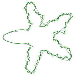
For instance, consider the three examples depicted in Figure 1. To generate random field samples, there are two components of that we can vary: the diffusion matrix and the potential. In Figure 1(a), we use a diffusion matrix to give the field preferred directions, more specifically it elongates field in the northwest-southeast direction. The potential is large over the continents and small over the oceans, effectively “turning off” the random field over land. In Figure 1(b), the potential is small in the front of the brain and large elsewhere, so that the field is only large in the front of the brain. Finally, Figure 1(c) shows the method used to generate a non-stationary random field in the one-dimensional case. To illustrate the value of the field at a point, we move it in the normal direction for a distance proportional to the value of the field. In all three cases, we see that the field behaves locally varying over the domain. With the suggested model, we can achieve preferred directions, local activation, and local deactivation.
The computational method we use to solve Equation 1, i.e., sample the random fields, is based on the surface finite element method (SFEM), a computational method pioneered by Dziuk (1988); Dziuk and Elliott (2013) and that has been used in the context of the generation of random fields in for instance Bonito et al. (2024); Jansson et al. (2022); Lang and Pereira (2023). Our main mathematical contribution is a strong convergence result. Using a functional calculus approach to the finite element discretization error, we obtain a strong rate of convergence of order , where for surfaces and for curves, and is a dimension-dependent logarithmic factor.
The SPDE approach to random fields and their approximation have been studied previously for both surfaces and Euclidean geometries, examples include Bonito et al. (2024); Borovitskiy et al. (2020); Bolin et al. (2020); Cox and Kirchner (2020); Jansson et al. (2022); Lang and Pereira (2023); Lindgren et al. (2011, 2022). However, to the best of our knowledge, we are the first to present a strong error analysis for the non-stationary case on hypersurfaces. Moreover, we achieve this without requiring an explicit approximation of the eigenfunctions of the elliptic operator, and contrary to for instance Borovitskiy et al. (2020), computing the eigenfunctions. In fact, the computation of eigenfunctions, with theoretical guarantees, is a notoriously difficult problem, see e.g., Boffi (2010). Our method circumvents this issue by introducing a Chebyshev approximation.
Our main contribution is a powerful, efficient, and flexible tool for the modeling and sampling of non-stationary random fields on curves and surfaces with proven accuracy. In particular, using tools from complex analysis and operator theory, we derive strong error bounds for approximations of arbitrary sufficiently smooth transformations of elliptic operators, where we do not require assumptions on the approximability of individual eigenfunctions.
The paper is structured as follows: In Section 2, we introduce the relevant deterministic framework. We provide the necessary background on geometry and functional analysis in Section 2.1. This is followed by a description of the main computational tool, surface finite elements in Section 2.2. Finally, Section 2.3 provides the relevant error estimates in the deterministic setting. In Section 3, we collect all material in the stochastic setting. We introduce first the class of considered random fields in Section 3.1 and their Galerkin–Chebyshev approximation in Section 3.2. The proof of its strong convergence is split into the SFEM error in Section 3.3 and the Chebyshev approximation error Section 3.4. For numerical confirmation of our theoretical results, we refer to our earlier work Lang and Pereira (2023) and the results presented in Bonito et al. (2024). The source code used to generate the figures is available at this address: https://github.com/mike-pereira/SFEMsim.
2. Deterministic theory: geometry, functional analysis and finite elements
Before we are able to approximate random fields on hypersurfaces, we need to introduce and partially extend the existing literature on surface finite element approximations due to so far unconsidered error bounds required in our stochastic setting. We introduce the functional analytic setting in Section 2.1, discuss surface finite element methods in Section 2.2 and show error bounds in the deterministic setting in Section 2.3.
2.1. Geometric and functional analytic setting
Let be a -dimensional () compact oriented smooth hypersurface () without boundary, i.e., for any , there exists an open set containing and a function such that on and
The tangent space of at is the -dimensional subspace of given by (where denotes the usual gradient of functions of and denotes the orthogonal complement in with respect to the standard Euclidean inner product.). Since is oriented, there exists a smooth map assigning to each point a unit vector perpendicular to the tangent space . Our hypersurface is a Riemannian manifold equipped with the metric that is the pullback of the Euclidean metric on . For instance, if , this results in the standard round metric.
Let be the gradient operator acting on differentiable functions of , and let denote the Laplace–Beltrami operator on . We denote by the surface measure on , and by the Hilbert space of -measurable square integrable complex-valued functions, equipped with the inner product defined by
The Sobolev spaces with smoothness index are then defined via Bessel potentials by
with corresponding norm . For , is defined as the space of distributions generated by
| (2) |
where is the smallest integer such that . In this case, the corresponding norm is given by . We set . The reader is referred to Herrmann et al. (2018), Strichartz (1983), Triebel (1985), and references therein for more details on Sobolev spaces defined using Bessel potentials.
In this work, we consider elliptic differential operators associated to bilinear forms given by
| (3) |
where for any the diffusion matrix is a real-valued, symmetric matrix such that for any , and if . In particular, since , is simply a matrix admitting as an eigenvector with some eigenvalue , and such that the eigenvalues , associated with its other eigenvectors are positive. Without loss of generality, we may assume that , meaning that , that the eigenvalues , are uniformly lower-bounded and upper-bounded on by positive constants, and that for any . Finally, we assume that is a real-valued function that satisfies for some .
Throughout this paper, let be coercive and continuous, i.e., there exist positive constants and such that for all ,
| (4) | |||
| (5) |
Following Yagi (2010, Equation (1.33)), gives rise to an associated elliptic differential operator defined weakly by
The spectral properties of this operator are detailed in the next proposition, which is proven in Appendix A.
Proposition 2.1.
Let be the coercivity constant defined in Equation 4. There exists a set of eigenpairs of consisting of a sequence of increasing real-valued eigenvalues with as , and forms an orthonormal basis of where each is real-valued.
Since the operator differs from the Laplace–Beltrami operator only by a zeroth-order potential term and a diffusion function in the second order term, switching between the two operators corresponds to a change of metric on . Therefore, the eigenvalue problem for is equivalent to that for the Laplace–Beltrami operator on equipped with a possibly rough metric if the coefficients of are not smooth. The results in Bandara et al. (2021) imply growth rates on the eigenvalues in accordance with Weyl’s law, and more specifically that there exist such that for any
| (6) |
As a last step in this subsection, we introduce nonlinear functions of which allow later in Section 3 for the definition of a variety of Gaussian random fields. For that, we call a function an -power spectral density if
-
1)
is extendable to a holomorphic function on .
-
2)
There exist constants and such that for all ,
(7)
Applying a power spectral density to results in a linear operator whose action on functions is defined by
| (8) |
where are the eigenpairs of defined in Proposition 2.1. A typical example is the function for and , which can be used to obtain Whittle–Matérn random fields (Lang and Pereira, 2023).
The goal of the remainder of this section is to study the approximation of functions of the form , where . Formally, if is well-defined on the spectrum of , then this is the solution to the partial differential equation .
2.2. SFEM–Galerkin approximation
The idea behind the surface finite element method, as introduced by Dziuk (1988), is to work on a polyhedral approximation of the surface that is in some sense close to the true surface . More precisely, fix and let be a piecewise polygonal surface consisting of non-degenerate simplices (for , triangles and for , line segments) with vertices on , and such that is the size of the largest simplex defined as the in-ball radius. The set of simplices making up the discretized surface is denoted by , thus meaning that
and we assume that for any two simplices in , it holds that their intersection is either empty, or a common edge or vertex.
Following (Dziuk and Elliott, 2013, Section 1.4.1), we assume that the triangulation is quasi-uniform, shape-regular, and that the number of simplices sharing the same vertex can be upper-bounded by a constant independent of . In turn, these two assumption imply that where denotes the number of vertices of .
The discrete surface is close to the true surface in the sense that is contained in a small neighborhood around defined as follows. First, note that can be seen as the boundary of some bounded open set with exterior normal . Then, following Dziuk and Elliott (2013, Section 2.3), we consider that there exists some (small) such that is contained in a so-called tubular neighborhood of defined by
where denotes the oriented distance function given by
We denote by the surface measure on , and by the Hilbert space of -measurable square integrable functions, equipped with the inner product defined by
Following (Bonito et al., 2020, Section 1.2.1), we denote by the area element given by , such that for all ,
| (9) |
where we next introduce the lift and its inverse denoted by and , respectively.
A key element of SFEM is that we can move between and using the so-called lift operator. To construct the lift operator, we note that for , and that for any , there exists a unique such that
where denotes the normal at to . In particular, this implies that any point can be uniquely described by the pair , and this procedure defines an isomorphism given by
Therefore, any function may be lifted to by . Likewise, the inverse lift of any function is given by . The procedure is illustrated in Figure 2 in the one-dimensional setting. Note that the points on the discretized surface are lifted along the normal to the surface .
The mapping is used to define the gradient of functions on (Dziuk and Elliott, 2013). More specifically, for a differentiable , the gradient is given by
| (10) |
where is the normal of and is the continuous extension of defined by . With this definition, the Laplace–Beltrami operator on can be defined by , and Sobolev spaces on are defined in complete analogy to those on .
The analogue of the bilinear form on is given by
| (11) |
where . As in Dziuk and Elliott (2013), we assume that there exists small enough, such that is coercive (and continuous) whenever . Unless stated otherwise, we now assume that this last condition on is fulfilled.
To conclude this subsection, we introduce the (linear) finite element space on . The finite element space is defined as the complex span of the standard real-valued nodal basis , where for any , is a polynomial of at most degree one taking the value at the -th vertex of and at all the other vertices, i.e.,
By construction, is a vector space of dimension . Its counterpart on is the lifted finite element space given by
On , we can, as on , associate to the bilinear form in Equation 11 a linear operator which maps any to the unique satisfying, for any , the equality
Similarly, if the bilinear form introduced in Equation 3 is restricted to , we can associate it to a linear operator that maps any to the unique that satisfies, for any , the equality
Since the bilinear forms and are coercive, positive definite, Hermitian and have real coefficients, these two operators are diagonalizable in the sense that they each give rise to a set of eigenpairs (Hall, 2013). On the one hand, there exists a sequence and an -orthonormal basis of such that
and similarly there exists a sequence and an -orthonormal basis of such that
In particular, using the same approach as in Proposition 2.1, we can assume that the eigenfunctions and are all real-valued. The eigenvalues of the operators , and are linked to one another through the following lemma, due to Bonito et al. (2018, Lemma 3.1), Bonito et al. (2024, Lemma 4.1) and Strang and Fix (2008, Theorem 6.1).
In the following, is shorthand for that there is a constant such that .
Lemma 2.2 (Eigenvalue error bounds).
Let , and denote the eigenvalues of the operators , and , respectively. Then,
| (12) |
and
| (13) |
Finally, we remark that the eigenvalues of can be linked to the eigenvalues of some classical finite element matrices. Let and be the so-called mass matrix and stiffness matrix, respectively, and defined from the nodal basis by
| (14) |
As defined, is a symmetric positive definite matrix and is a symmetric positive semi-definite matrix. Let then be an invertible matrix satisfying . Then, by Lang and Pereira (2023, Corollary 3.2), the eigenvalues are also the eigenvalues of the matrix defined by
| (15) |
Besides, if denotes the vector-valued function given by , then the mapping , defined by
is an isomorphism whose inverse maps the eigenfunctions to (orthonormal) eigenvectors of . This means in particular that can also be written as
| (16) |
where .
2.3. Deterministic error analysis
Based on the introduced framework, we are now in place to quantify the error between functions of the operators , and . Let be the -projection onto and let the -projection onto . We note that the operators , , and define norms that are equivalent to the standard Sobolev norms, i.e.,
| (19) |
for all , and all and .
With that at hand we are ready to state our main result in this section.
Proposition 2.3.
Let be an -power spectral density. Then, there is a constant such that for all
To prove this proposition we rely on a representation of functions of operators based on Cauchy–Stieltjes integrals, which are constructed as follows. Since the sesquilinear form defined by is continuous and coercive, the associated operators and are sectorial with some (common) angle (Yagi, 2010, Theorem 2.1). Therefore, the spectra of and are contained in the complement of the set , as illustrated in Figure 3(a), and the following inequalities are satisfied for any (cf. Yagi (2010, Equation (2.2))):
| (20) |
where is a generic constant. Note in particular that by definition, is contained in the resolvent sets of and , and that any power spectral density is bounded, holomorphic and satisfies the inequality for any . Hence, the operators and can be defined as functional calculi of the operators and as (Yagi, 2010, Chapter 16, Section 1.2) by
| (21) |
where is any integral contour surrounding the spectra of and and contained in . In particular, these new definitions of functions of operators are independent of the choice of , and coincide with the spectral definitions previously introduced in Equation 8 (cf. e.g. (Yagi, 2010, Remark 2.7)).
In the remainder, we split the contour into
| (22) |
where is parametrized by for , by for and by for with (see Figure 3(b) for an illustration). We use this contour to prove Proposition 2.3, while relying on the following bounds for the resolvent error along . The proof is included in Appendix A and is an adaption of results from Fujita and Suzuki (1991) and Bonito et al. (2024).
Lemma 2.4.
For any , , and ,
We now provide a proof for Proposition 2.3.
Proof of Proposition 2.3.
Let . For any , set , which yields, using the integral representations of and ,
The definition of and its parametrization allow to decompose the integral as
where we recall that and . Taking norms on both sides of this equality and using the triangle inequality then gives
Let us start by bounding . We apply Equation 7 and Lemma 2.4 with to obtain
To bound , we distinguish between the three cases , and . When , we apply Equation 7 and Lemma 2.4 with to get
For , recall that and assume without loss of generality that . We split with
Using Equation 7 and Lemma 2.4 with we bound by
We proceed in the same manner to bound , but use Lemma 2.4 with ,
For and the same splitting we obtain for with Lemma 2.4 for
Assuming again and , we finally bound
The bound for is obtained in the same way as in the case . Hence, for .
Finally, note that by symmetry, satisfies the same bounds as , which finishes the proof adding up all terms. ∎
A result similar to Proposition 2.3 can be derived to quantify the error between functions of the operators and . To do so, we note that since is continuous and coercive, the associated operator is also sectorial with some angle in . Hence, without loss of generality, the angle can be assumed to be large enough to ensure that Equation 20 also holds for , i.e. that for any ,
| (23) |
and that an integral representation similar to Equation 21 also holds for , namely:
Proposition 2.5.
Let be an -power spectral density with . There exists a constant such that, for any ,
| (24) |
This proposition can be seen as an extension of Bonito et al. (2024, Lemma 4.4) relying on extensions of the estimates proven in Bonito et al. (2024, Lemma A.1). Its proof is similar and therefore postponed to Appendix B.
3. Stochastic theory: random fields on surfaces and convergence of SFEM approximation
In this section, we introduce random fields and white noise on surfaces, thus allowing us to make sense of Equation 1 in Section 1. Further, we give approximation methods based on SFEM and prove strong error bounds.
3.1. Random fields on surfaces
Let be a complete probability space. We are interested in Gaussian random fields on defined as -valued random variables through expansions of the form
| (25) |
where denotes a real-valued orthonormal basis of composed of eigenfunctions of the operator (cf. Proposition 2.1), and is a sequence of real Gaussian random variables such that for any and . As such, can be seen as en element of the Hilbert space of -valued random variables, to which we associate the inner product (and norm ) defined by
Finally, in analogy to Equation 25, we formally define the Gaussian white noise on by the expansion
| (26) |
where is a sequence of independent real standard Gaussian random variables. We observe that even though this expansion does not converge in , it does however converge in for . Moreover, we have that for any , the expansion converges in . Further, defines a complex Gaussian variable with mean , and for any , . As such, the Gaussian white noise (26) can be interpreted as a generalized Gaussian random field over .
Circling back to the class of random fields defined in Section 1, we can now make sense of Equation 1 through Equation 8 and Equation 26, thus yielding the definition
| (27) |
which results in for any such that . Note in particular that all summands in Equation 27 are real-valued functions, and that therefore is real-valued. In Figure 4 we illustrate the influence of the parameter choices on the resulting field on for generalized non-stationary Whittle–Matérn fields on
where . By selecting and with one recovers the classical, stationary Whittle–Matérn fields studied in various settings in for instance Cox and Kirchner (2020); Bolin et al. (2020); Bonito et al. (2024); Lindgren et al. (2011); Jansson et al. (2022); Whittle (1963). In Figures 4(a) and 4(b) we show this case with for a rougher field with and a smoother one with , respectively.
Two non-stationary fields are shown in Figure 4(c) and Figure 4(d), obtained by varying the coefficient functions and and setting . In Figure 4(c), we keep but use
resulting in the observed localized behavior, where the field is essentially turned off in the region with large . More specifically, describes the local correlation length, where a large corresponds to a small correlation length around .
Finally, setting constant again, we show the influence of varying parameters in Figure 4(d). To derive suitable coefficients, we select a smooth function and compute its gradient as well as its skew-gradient given by at each point . We set for fixed , for any . Here, the inner product refers to the Riemannian inner product associated with the standard round metric on . Since and both are in , is a linear mapping from into itself. Further, as is perpendicular to , by selecting and , we obtain a field that is elongated either orthogonally to the level sets of (large , small ) or tangentially to the level sets (small , and large ). To generate Figure 4(d), we selected , i.e., the function returning the second coordinate in Cartesian coordinates, and .
3.2. Approximation of random fields with surface finite elements
Let be an -power spectral density with . Following the approach presented by Lang and Pereira (2023), the field is approximated by an expansion similar to that of Equation 27, but involving only quantities defined on the polyhedral surface . More precisely, we define the SFEM–Galerkin approximation of the field by the relation
| (28) |
where is a sequence of independent standard Gaussian random variables, whose precise definition is clarified later in this section, and are the eigenpairs of introduced in Section 2.2. Then, as proven in Lang and Pereira (2023, Theorem 3.4), can be decomposed in the nodal basis of as
where the weights form a centered Gaussian vector which covariance matrix can be expressed using the matrices and introduced in Equations 14 and 15 as follows:
| (29) |
and, following Equation 16, the function of matrix is defined as
| (30) |
Note that sampling the weights , and therefore the field , using directly the expression of their covariance matrix requires in practice to fully diagonalize (since Equation 29 involves a function of a matrix). Such an operation would result in a prohibitive computational cost (of order operations). To avoid this cost, we use the Chebyshev trick proposed by Lang and Pereira (2023, Section 4), and approximate by the field defined by
| (31) |
where is a Chebyshev polynomial approximation of degree of over an interval containing all the eigenvalues of (which we recall, coincide with the eigenvalues of ). Such an interval can be obtained as follows. On the one hand, one can take . On the other hand, following Lang and Pereira (2023), a candidate for is obtained by applying the Gershgorin circle theorem to .
Since is defined by just replacing the power spectral density by the polynomial , its expansion into the nodal basis,
is such that the weights now form a centered Gaussian vector with covariance matrix given by
| (32) |
Hence, the matrix function in Equation 29 is now replaced by a matrix polynomial . This eliminates the eigendecomposition need associated with matrix functions and therefore speeds up the computations. Indeed, the weights can be sampled through
where are independent standard Gaussian random variables, and the matrix-vector product by can be computed iteratively while just requiring products between and vectors. In the next two subsections, we provide error estimates quantifying the error between our target random field and its successive SFEM and polynomial approximations by and .
3.3. Error analysis of the SFEM discretization
We start with analyzing the error between the random field defined on and its SFEM approximation , as stated in the next theorem.
Theorem 3.1.
Let be an -power spectral density with . Then, there exists , such that for any the strong approximation error of the random field by its discretization satisfies the bound
| (33) |
where if , if , and otherwise.
To prove the strong error estimate, we rely on the deterministic error bounds proven in the previous section, and on several intermediate approximations of defined on the spaces (i.e., on ) and (i.e., on ). These intermediate approximations require in turn to define approximations of the Gaussian white noise on the spaces and .
We first define on (i.e., on ), the projected white noise as
| (34) |
where we recall that denotes an orthonormal basis of eigenfunctions of , and for any , we take . In particular, this last relation implies (by definition of the white noise ) that are independent standard Gaussian random variables.
Remark 3.2.
By injecting the representation (26) of in the definition of , we get that can itself be formally represented by . This explains why we refer to it as a projected white noise.
Based on , we can then introduce a first approximation, on the space , of the field . We denote this approximation by and define it in analogy to Equation 27 as
| (35) |
Now, on the space , we define two white noise approximations and which are based on the projected white noise :
where is the ratio of area measures introduced in Section 2.2. On the one hand, we associate to an approximation of the field on , which we define in analogy to Equation 36 as
On the other hand, by expanding and in the orthonormal basis of eigenfunctions of , we obtain alternative representations of these fields, and we can draw a link between and the SFEM–Galerkin approximation , as stated in the next lemma.
Lemma 3.3.
The noises and can be written as
where and are multivariate normal with mean and respective covariance matrices and . In particular, it holds that the SFEM–Galerkin approximation defined in Equation 28 satisfies
| (36) |
where we take for any , .
Proof.
As , we can expand it in the orthonormal basis to get
where . Then, by definition of , of and since , we further get for any ,
Therefore, by definition of the white noise , we can conclude that for any , is normally distributed with mean , and that
Hence, is indeed multivariate normal (any linear combination of the being Gaussian by definition of ) with mean and covariance matrix .
Similarly, since , we can write again
where , and the same computations as before yield that . Hence, we can conclude this time that for any , is also normally distributed with mean , and that
by orthonormality of . In conclusion, is indeed multivariate normal with mean and covariance matrix . In particular, this means that are independent standard Gaussian variables.
We now circle back to proving Theorem 3.1. Using the intermediate approximations and and the equivalence of the norms on and , we can upper-bound the error between the field and its SFEM–Galerkin approximation by
We derive error estimates for each one of the three terms obtained in the last inequality. We start with the term .
Lemma 3.4.
It holds that
where if and , otherwise.
Proof.
Our aim is to bound the error between and , where we remark in particular that and (cf. Remark 3.2). Let , and let , so that . Further, define the function . Note that, since is an -power spectral density and since decays as
is a -power spectral density. Now, by definition of ,
so that the triangle inequality yields
where we take
For the term , note that by Bonito et al. (2024, Lemma 4.2),
In particular, is in and an application of Proposition 2.3 yields that
where
For , we first write , where . Further, following the definition of in Equation 34, we have where . Note in particular that both and are real-valued (since the eigenbases and are real-valued). Thus,
where we use the orthonormality of the eigenfunctions. Note that
First, by the independence of the sequence and eigenpairs of ,
Similarly, and using the fact that is an eigenpair of ,
and
This implies that by Proposition 2.3,
where
Hence, it holds that
It remains to bound . To this end, recall Equation 12 and Equation 6 which yield that
where we used in the last inequality that . We obtain
with
We conclude that
and in particular,
where we take . We have two cases. On the one hand, if then, since , we also have and therefore , and (given that ). On the other hand, if , then and and therefore . In turn, this means that . Hence, in both cases
and we conclude that
The result follows by inserting the definition of . ∎
For the error between and we get the following estimate, inspired by Bonito et al. (2024, Lemma 4.4).
Lemma 3.5.
It holds that
Proof.
Let . We note that is an -valued random variable. Therefore, we can apply Equation 24 to realizations of , and take the expectation on both sides to get
We then distinguish two cases. First, if , then we note that since . Besides, Bonito et al. (2024, Lemma 4.2) yields that for all , there is a constant such that
| (37) |
Hence, using estimate (37), we conclude that
If now , since , we have . We then note that by the proof of Bonito et al. (2024, Lemma 4.2), for any
Apply now Equation 6 to see that
meaning that for any ,
In particular, taking yields
which concludes the proof. ∎
Finally, for the error between and we get the following estimate.
Lemma 3.6.
It holds that there is a constant such that
Proof.
To prove this statement, we note that, using the same notations as the ones in the proof of Lemma 3.3,
where we applied the orthogonality of the eigenfunctions in the last step. Now, following the definition of and given in the proof of Lemma 3.3,
Besides, for all , it holds that
Therefore,
where Dziuk and Elliott (2013, Lemma 4.1) was applied in the final step. We conclude that
and it remains to show that is bounded by a constant. To this end, we use Lemma 2.2, which implies that there exists some constant such that
Recall then that the mesh size satisfies , where . Without loss of generality, let us further assume that . Now, by the growth assumption on ,
Using Equation 12 and Equation 6, we bound
where denotes the Riemann zeta function. Thus, is bounded by a constant and
which proves the lemma. ∎
Equipped with the estimates derived in Lemmas 3.6, 3.5 and 3.4 we are ready to prove Theorem 3.1.
Proof of Theorem 3.1.
By summing the three estimates derived in Lemmas 3.6, 3.5 and 3.4, we get
Let then be the quantity defined by , which satisfies
If , we have and , and therefore . Similarly, if , it holds and , and therefore . Finally, for , , and , and therefore . In conclusion, we obtain for any , which in turn yields
Having bounded the SFEM error, we are now ready to derive the additional error associated with the Chebyshev approximation which we use to compute SFEM–Galerkin approximations in practice.
3.4. Error analysis of the Chebyshev approximation
To bound the error between and , we can directly apply Lang and Pereira (2023, Theorem 5.8). We obtain the following result.
Theorem 3.7.
Let be the interval on which the Chebyshev polynomial approximation is computed, and let . Then, there exists a constant such that the error between the discretized field and its approximation is upper-bounded by
| (38) |
with . In particular, setting and , the error is bounded by
| (39) |
for some constant proportional to .
Proof.
Let be the ellipse centered at , with foci and , and semi-major axis . In particular, note that and for any , . Hence, since is a power spectral density, by definition is holomorphic and bounded inside . We can then adapt the same proof as in Lang and Pereira (2023, Theorem 5.8) to obtain the stated proposition. ∎
For a fixed mesh size , the approximation error converges to as the order of the polynomial approximation goes to infinity. Choosing as a function of that grows fast enough then allows us to ensure the convergence of the approximation error as goes to infinity (Lang and Pereira, 2023, Section 5.2).
References
- Bandara et al. (2021) L. Bandara, M. Nursultanov, and J. Rowlett, Eigenvalue asymptotics for weighted Laplace equations on rough Riemannian manifolds with boundary, Ann. Sc. Norm. Super. Pisa Cl. Sci. (2021), 1843–1878.
- Boffi (2010) D. Boffi, Finite element approximation of eigenvalue problems, Acta Numer. 19 (2010), 1–120.
- Bolin et al. (2020) D. Bolin, K. Kirchner, and M. Kovács, Numerical solution of fractional elliptic stochastic PDEs with spatial white noise, IMA J. Numer. Anal. 40 (2020), 1051–1073.
- Bonito et al. (2020) A. Bonito, A. Demlow, and R. H. Nochetto, Finite element methods for the Laplace–Beltrami operator, Handbook of Numerical Analysis, vol. 21, pp. 1–103, Elsevier, 2020.
- Bonito et al. (2018) A. Bonito, A. Demlow, and J. Owen, A priori error estimates for finite element approximations to eigenvalues and eigenfunctions of the Laplace–Beltrami operator, SIAM J. Numer. Anal. 56 (2018), 2963–2988.
- Bonito et al. (2024) A. Bonito, D. Guignard, and W. Lei, Numerical approximation of Gaussian random fields on closed surfaces, Comput. Appl. Math. In press (2024).
- Borovitskiy et al. (2020) V. Borovitskiy, A. Terenin, P. Mostowsky, and M. P. Deisenroth, Matérn Gaussian processes on Riemannian manifolds, Advances in Neural Information Processing Systems 33, 2020.
- Cox and Kirchner (2020) S. G. Cox and K. Kirchner, Regularity and convergence analysis in Sobolev and Hölder spaces for generalized whittle–matérn fields, Numer. Math. 146 (2020), 819–873.
- Dziuk (1988) G. Dziuk, Finite elements for the Beltrami operator on arbitrary surfaces, Partial differential equations and calculus of variations, vol. 1357 of Lecture Notes in Math., pp. 142–155, Springer, Berlin, 1988.
- Dziuk and Elliott (2013) G. Dziuk and C. M. Elliott, Finite element methods for surface PDEs, Acta Numer. 22 (2013), 289–396.
- Farag (2014) A. A. Farag, Biomedical Image Analysis: Statistical and Variational Methods, Cambridge University Press, Cambridge, 2014.
- Fujita and Suzuki (1991) H. Fujita and T. Suzuki, Evolution problems, Handbook of Numerical Analysis, pp. 789–928, Elsevier, 1991.
- Hall (2013) B. C. Hall, Quantum Theory for Mathematicians, Springer, New York, 2013.
- Herrmann et al. (2018) L. Herrmann, A. Lang, and C. Schwab, Numerical analysis of lognormal diffusions on the sphere, Stoch PDE: Anal. Comp. 6 (2018), 1–44.
- Jansson et al. (2022) E. Jansson, M. Kovács, and A. Lang, Surface finite element approximation of spherical Whittle–Matérn Gaussian random fields, SIAM J. on Sci. Comput. 44 (2022), A825–A842.
- Lang and Pereira (2023) A. Lang and M. Pereira, Galerkin–Chebyshev approximation of Gaussian random fields on compact Riemannian manifolds, BIT Numer. Math. 63 (2023), 51.
- Lindgren et al. (2022) F. Lindgren, D. Bolin, and H. Rue, The SPDE approach for Gaussian and non-Gaussian fields: 10 years and still running, Spat. Stat. 50 (2022), 100599.
- Lindgren et al. (2011) F. Lindgren, H. Rue, and J. Lindström, An explicit link between Gaussian fields and Gaussian Markov random fields: The stochastic partial differential equation approach, J. R. Stat. Soc. Ser. B Methodol. 73 (2011), 423–498.
- Marinucci and Peccati (2011) D. Marinucci and G. Peccati, Random Fields on the Sphere. Representation, Limit Theorems and Cosmological Applications, vol. 389 of London Mathematical Society Lecture Note Series, Cambridge University Press, Cambridge, 2011.
- Shubin (2001) M. A. Shubin, Pseudodifferential Operators and Spectral Theory, Springer, Berlin, 2001.
- Strang and Fix (2008) G. Strang and G. Fix, An Analysis of the Finite Element Method, Wellesley-Cambridge Press, Wellesley, MA, 2008.
- Strichartz (1983) R. S. Strichartz, Analysis of the Laplacian on the complete Riemannian manifold, J. Funct. Anal. 52 (1983), 48–79.
- Taylor (2011) M. E. Taylor, Partial Differential Equations I. Basic Theory, vol. 115 of Applied Mathematical Sciences, Springer, New York, 2011.
- Triebel (1985) H. Triebel, Spaces of Besov–Hardy–Sobolev type on complete Riemannian manifolds, Ark. Mat. 24 (1985), 299–337.
- Whittle (1963) P. Whittle, Stochastic processes in several dimensions, Bull. Inst. Int. Stat. 40 (1963), 974–994.
- Yagi (2010) A. Yagi, Abstract Parabolic Evolution Equations and Their Applications, Springer Monographs in Mathematics, Springer, Berlin, 2010.
Appendix A Deterministic proofs
A.1. Proof of Proposition 2.1
Proof.
A standard result in the spectral theory of elliptic operators on compact Riemannian manifolds (see e.g. (Shubin, 2001, Section 8)) ensures that there exists a set of eigenpairs of such that with as , and is an orthonormal basis of composed of possibly complex-valued functions.
Hence, let us prove that and that we can build an orthonormal basis of such that each is real-valued and an eigenfunction of with eigenvalue . On the one hand, by definition of , and , we obtain
where for the last two inequalities we used the coercivity of and the definition of the -norm.
On the other hand, let be one of the eigenvalues of , and the associated eigenspace. Following again the results from (Shubin, 2001, Section 8), we get that , and that if is another eigenvalue of , then and are orthogonal. Besides, is in fact generated by the set , where is finite (since ).
Take then . Hence, for any , . But also, by definition of ,
where used the fact that is a real symmetric matrix and is real-valued for the first two equalities. Consequently, we also have , and so, the real-valued functions and (corresponding to real and imaginary parts of ) are also in .
Circling back to the orthonormal basis of , we consider the set of real-valued functions , and the subspace generated by . In particular . By applying the Gram–Schmidt orthogonalization process to , we get an orthonormal basis of which by construction is composed of real-valued functions (since is composed of real-valued functions). Let us show that is in fact a basis of , or equivalently that .
We proceed by contradiction. Assume that . This means in particular that the orthogonal complement of in , denoted by , is not reduced to . Let then . By linearity, we have, for any , , since . Hence, since and is an orthonormal basis of , it must hold that , which contradicts our initial claim. Consequently, , and therefore is an orthonormal basis of .
Finally, by repeating the construction above to each eigenspace associated with distinct eigenvalues, and concatenating the obtained bases, we obtain an orthonormal basis (due to the fact that these eigenspaces are orthogonal to one another and span ). Each element in this basis is an eigenfunction of since it is built from a given eigenspace, and is a real-valued function. This concludes our proof. ∎
A.2. Proof of Lemma 2.4
Proof.
Let us start by proving the following claims: for any , ,
| (40) | |||
| (41) |
We omit the proof of Equation 41 and refer the reader to Fujita and Suzuki (1991, Theorem 5.1), where the proof may be adapted verbatim.
To prove Equation 40, we can largely proceed as in Fujita and Suzuki (1991, Theorem 7.1), substituting the Euclidean elliptic regularity estimates and interpolation bounds with their surface counterparts, see for instance Taylor (2011, Chapter 11), Dziuk and Elliott (2013, Lemma 4.3) and Bonito et al. (2024, Equation (4.8)). We must in essence only adapt Fujita and Suzuki (1991, Lemma 7.1) to also hold for , as their estimate only holds for . In other words, we must show that for any , where , there is a constant such that for all ,
| (42) |
To prove this inequality, note that by coercivity of ,
Let then . Since the only requirement on was that , we can then write
since if . Therefore,
This last inequality implies in particular that and therefore that
Using once again that and that , we deduce that
by the reverse triangle inequality. To conclude, we have proven that the relation (42) holds and equipped with this estimate, we can proceed as in the proof of Fujita and Suzuki (1991, Theorem 7.1) and obtain Equation 40.
Finally, by interpolating between the bounds obtained in Equations 40 and 41, we obtain that, for any ,
Appendix B Error between functions of discrete operators
The aim of this section is to prove Equation 24. To do so, we rely on a geometric consistency estimate, and on extensions of the results of Bonito et al. (2024, Lemma A.1), which we start by stating and proving.
B.1. Geometric consistency estimate
The following geometric consistency estimate quantifies the error between the bilinear forms and . Its proof is a straightforward adaptation of the proof of Dziuk and Elliott (2013, Lemma 4.7) to account for the diffusion matrix .
Lemma B.1.
There is a constant such that for all and ,
| (43) |
Proof.
We first note that, by definition of , for any , and any , defines an inner product on . We denote by the usual Euclidean norm of vectors of and by the norm defined by , .
Let (resp. ) be the orthogonal projection onto the tangent planes of (resp. ), and let be the extended Weingarten map of (cf. Dziuk and Elliott (2013, Definition 2.5)). Recall in particular that for any , meaning in particular that . Finally, we introduce the map defined as
where is the oriented distance function restricted to and introduced in Section 2.2. On the one hand, note that for any ,
which gives, after integrating both sides over and using Equation 9,
| (44) |
Let then be the Hermitian form defined for any by
| (45) | ||||
Note that following Equations 44 and 9, satisfies for any the equality . Therefore, for any , we bound
| (46) | ||||
We now bound these two terms. Recall that Dziuk and Elliott (2013, Lemma 4.1) shows
| (47) |
Hence, since takes positive values,
which in turn gives (using the Cauchy–Schwartz inequality and Equation 47),
| (48) |
To bound the other term, we first introduce for any the notation . Then we have
By Equation 47 and since has bounded eigenvalues over , we obtain
| (49) |
where the constant in the inequality is independent of the location on . We split the first term on the right into
Since by Dziuk and Elliott (2013, Lemma 4.1) and is defined independently of , we conclude that
| (50) |
We notice that , since by definition of , , which implies
Using that by the proof of Dziuk and Elliott (2013, Lemma 4.1), we deduce that . Injecting this inequality into Equation 50, and the resulting inequality into Equation 49, we conclude that
This allows us to write
where maps any to the smallest eigenvalue of associated with an eigenvector in . This last inequality is a consequence of the fact that by construction and using the characterization of eigenvalues through Rayleigh quotients. Since the non-zero eigenvalues of are uniformly bounded above and below by positive constants, we conclude that
Then, using the Cauchy–Schwartz inequality yields
| (51) |
Inserting the derived bounds Equation 48 and Equation 51 into Equation 46, we derive
Note that for any ,
so we obtain
Finally, due to Equation 5,
and the result follows. ∎
B.2. Norm and error estimates of discrete operators
We now prove some estimates for the norm of shifted inverses of the operators and , and for the error between inverses of these two operators. These results can be seen as extensions of the ones stated in Bonito et al. (2024, Lemma A.1).
Lemma B.2.
Let and be arbitrary. Then, for all , for any , and any ,
| (52) | |||
| (53) | |||
| (54) | |||
| (55) |
Proof.
We start with the proof of Equation 52. To this end, let and . For any and , we expand
implying that
Hölder’s inequality yields
| (56) | ||||
Let , then we obtain by Equation 20 that
Hence, adding and subtracting yields
Combining this estimate with Equation 56, we get for any
| (57) |
yielding for any that
| (58) | ||||
where we applied Equation 57 with in the last step. Hence, we retrieve Equation 52.
Next, to prove Equation 53, we first observe that the estimates in Equation 57 and Equation 58 carry over to the case when is used instead of , as the proof in essence is a standard manipulation of a finite eigenexpansion. In particular, we obtain (by taking and )
| (59) |
Now, Equation 59 combined with the equivalence of norms in Equation 19, yields that
which shows Equation 53.
To bound Equation 54, we apply Equation 57 with to obtain
Finally, to prove the bound in Equation 55, we rely on the geometric consistency estimate of Lemma B.1. Let and let . Note that by definition of ,
for all . Likewise, for we obtain
for all , where we used the definition of in the last step. Let us now select a fixed, but arbitrary, . Then, by combining the last two equations,
meaning that an application of Lemma B.1 results in the bound
| (60) |
Further, note that for any , the equivalence of norms (19) gives
| (61) |
where the last equality comes from the definition of . And similarly, for any , we have
| (62) |
Then, applying the triangle inequality to the (last) right-hand side of Equation 61 gives
where we used Equation 62 and Lemma B.1 to derive the second inequality. This means in particular that there exists independent of such that . Recall that for some small enough. Assuming that especially yields , which allows us to conclude that
| (63) |
Now, applying successively Equation 62 and Equation 60 with , we obtain
where the last inequality is derived from applying Equation 63. Therefore, we end up with
where the equivalence of norms (19) together with the definition of are used in the final step. This concludes the proof of Equation 55. ∎
B.3. Proof of Equation 24
Based on the results in the previous subsections, we can now move on to the proof of Equation 24.
Proof.
Let . We introduce the inverse lift operator which maps any to . Let then . Note that by the integral representations of the operators (21)
where we take for any , . Similarly, as in the proof of Proposition 2.3, we use the splitting (22) of and the triangle inequality to deduce that
| (64) | ||||
where we take and . For , let us then introduce the quantity
so that Equation 64 may be rewritten as and in particular, for any .
We now fix and bound the term . First, for any , we rewrite and split
where we take and . Hence, by the triangle inequality,
| (65) |
We first bound . Using successively Equation 23 and the geometric estimates in Bonito et al. (2018, Corollary 2.2) results in
Using then Equation 54, we conclude that, for any ,
| (66) |
Using Equations 67 and 66 with together with Equation 65 gives
which yields in turn (since is an -power spectral density)
since . Finally, since this inequality holds for any , we retrieve the claim (24) using Equation 64.
∎