CERN-TH-2024-064, P3H-24-036, PSI-PR-24-13, SI-HEP-2024-14, TTP24-017, ZU-TH 28/24
Heavy-to-light form factors to three loops

Abstract

We compute three-loop corrections of $\mathcal{O}(\alpha_{s}^{3})$ to form factors with one massive and one massless quark coupling to an external vector, axialvector, scalar, pseudoscalar, or tensor current. We obtain analytic results for the color-planar contributions, for the contributions of light-quark loops, and the contributions with two heavy-quark loops. For the computation of the remaining master integrals we use the “expand and match” approach which leads to semi-analytic results for the form factors. We implement our results in a Mathematica and a Fortran code which allows for fast and precise numerical evaluations in the physically relevant phase space. The form factors are used to compute the hard matching coefficients in Soft-Collinear Effective Theory for all currents. The tensor coefficients at light-like momentum transfer are used to extract the hard function in $\bar{B}\to X_{s}\gamma$ to three loops.

1 Introduction

Form factors are the basic building blocks of scattering amplitudes in quantum field theories. Most prominently, they represent the bulk of virtual corrections to physical observables. The form factors for two massless external particles coupling to an external current have been computed up to four-loop order in QCD and QED for various combinations of particles and currents [1, 2, 3, 4, 5, 6, 7, 8, 9, 10, 11, 12, 13, 14, 15, 16, 17, 18, 19]. The heavy quark form factors, i.e. two fermions with the same mass coupling to a current, were known at the two-loop level for a long time [20, 21, 22, 23, 24, 25, 26, 27, 28, 29, 30, 31, 32] and partial three-loop results became available over the last decade [29, 33, 34, 35, 32, 36, 37]. Recently, the three-loop corrections for the vector, axialvector, scalar, and pseudoscalar currents were completed semi-analytically [38, 39, 40].

The heavy-to-light form factors of a heavy and a light fermion are especially relevant for decays of heavy quarks such as $t\to bW^{*}$, $b\to cW^{*}$, and $b\to uW^{*}$ or the production of a single top quark through the $t$-channel process. Specializing to QED, they also contribute to the muon decay in the Fermi theory, see e.g. Refs. [41, 42]. For some of the applications, neglecting the mass of the light fermion is a good first approximation in which the form factors were known to two-loop order for some time [43, 44, 45, 46]. Only a few years ago the full mass dependence of the heavy-to-light form factor became available at $\mathcal{O}(\alpha_{\text{s}}^{2})$ [50, 51]. Neglecting the light fermion mass, the color-planar corrections at $\mathcal{O}(\alpha_{\text{s}}^{3})$ to the vector, axialvector, scalar, and pseudoscalar form factors were computed recently [52, 53].

In this paper we compute the three-loop corrections to the heavy-to-light form factors in full QCD, still neglecting the mass of the light fermion. We reproduce the analytic results of Ref. [53] in the color-planar limit and extend it to the tensor form factors. Furthermore, we provide analytic results for the contributions of light-fermion loops and the contributions with two heavy-fermion loops for all form factors. For the remaining color factors we present semi-analytic results in terms of expansions around kinematic points following the strategy of Ref. [54] which was already applied to the three-loop corrections to the massive form factors in Refs. [38, 39, 40]. We restrict ourselves to the physically interesting regions relevant for the heavy-fermion decay and the heavy-fermion production in the $t$-channel. Furthermore, we present results for generic external currents. The specification to vertices appearing in the Standard Model or other theories of interest is straightforward. We provide our analytic results in the form of ancillary files accompanying this paper, and the numeric results for the full form factors as Mathematica and Fortran programs which perform an interpolation based on a dense grid [55].

The QCD form factors can be used to compute the hard matching coefficients to Soft-Collinear Effective theory (SCET) [56, 57, 58, 59] at leading power in the SCET expansion. The infrared divergences still present in the QCD form factors are removed during the procedure of infrared subtraction, yielding finite SCET matching coefficients. While their one-loop expressions have been computed in the founding SCET papers (see also Ref. [60]), the two-loop coefficients for the vector and axial vector current were computed in Refs. [43, 44, 45, 46]. In Ref. [61] the results were extended to the scalar and tensor currents. In the present paper the matching coefficients are computed to three-loop order for all currents considered.

An immediate application of the matching coefficients of the tensor current at light-like momentum transfer concerns the inclusive decay $\bar{B}\to X_{s}\gamma$. In a SCET-based approach, the decay rate is formulated in a factorized form as the product of a hard function times a convolution of a jet with a soft function [62, 63, 64]. While the latter two are known to three loops already [65, 66, 67, 68], the hard function has to date only been evaluated to two loops [69, 70, 71]. With the three-loop matching coefficients at hand we close this gap and compute the three-loop QCD correction to the hard function in $\bar{B}\to X_{s}\gamma$.

In the recent study [71], the authors claim the performance of a next-to-next-to-next-to-leading-logarithmic analysis of the photon energy spectrum in $\bar{B}\to X_{s}\gamma$ including three-loop corrections to the renormalization-scale independent part of the hard, jet and soft functions in SCET (i.e. a study to N³LL^′ accuracy). However, for the hard function this piece has only become available with the calculation presented here. In Ref. [71] the missing numerical coefficient at three loops was treated as a nuisance parameter. Our explicit three-loop calculation shows that the exact numerical value of the parameter in question lies more than a factor of two outside the variation region assumed in Ref. [71].

The remainder of this paper is structured as follows: In Section 2 we introduce the form factors and discuss their renormalization, the infrared subtraction, as well as the Ward identities of the currents which relate some of the form factors. Our calculational strategy is described in Section 3. We then present our results and discuss the analytic and numeric results in Section 4 and 5, respectively. The hard function in $\bar{B}\to X_{s}\gamma$ is presented in Section 6. We conclude in Section 7. In the Appendix we present explicit results for the projectors to all form factors. Furthermore, we describe the program FFh2l where our results are implemented and which allows for a fast and precise numerical evaluation.

2 Form factors

2.1 Currents and form factors

The theoretical framework used for our calculation is QCD supplemented with external currents formed by a heavy ($Q$) and a light quark field ($q$). In this paper we consider the vector, axialvector, scalar, pseudoscalar, and tensor currents

$$j_{\mu}^{v} = \bar{\psi}_{Q}\gamma_{\mu}\psi_{q}\,,$$

$$j_{\mu}^{a} = \bar{\psi}_{Q}\gamma_{\mu}\gamma_{5}\psi_{q}\,,$$

$$j^{s} = \bar{\psi}_{Q}\psi_{q}\,,$$

$$j^{p} = \mathrm{i}\bar{\psi}_{Q}\gamma_{5}\psi_{q}\,,$$

$$j_{\mu\nu}^{t} = \mathrm{i}\bar{\psi}_{Q}\sigma_{\mu\nu}\psi_{q}\,,$$ (1)

where $\sigma_{\mu\nu}={\rm i}[\gamma^{\mu},\gamma^{\nu}]/2$ is anti-symmetric in the indices $\mu$ and $\nu$. The wave functions of the heavy and light quark fields are denoted by $\psi_{Q}$ and $\psi_{q}$, respectively. We use the currents from Eq. (1) to construct vertex functions $\Gamma(q_{1},q_{2})$ via

$$\int\frac{\mathrm{d}^{4}y}{(2\pi)^{4}}\,\mathrm{e}^{\mathrm{i}q\cdot y}\langle\psi^{\text{out}}_{Q}(q_{2},s_{2})|j^{x}(y)|\psi^{\text{in}}_{q}(q_{1},s_{1})\rangle=\bar{u}(q_{2},s_{2})\Gamma(q_{1},q_{2})u(q_{1},s_{1})\,,$$ (2)

which are independent of the spin indices $s_{1}$ and $s_{2}$ and which can be decomposed into scalar form factors. We follow the notation introduced in Ref. [39] and define them as

$$\Gamma_{\mu}^{v}(q_{1},q_{2}) = F_{1}^{v}(q^{2})\gamma_{\mu}-\frac{\rm i}{m}F_{2}^{v}(q^{2})\sigma_{\mu\nu}q^{\nu}+\frac{2}{m}F_{3}^{v}(q^{2})q_{\mu}\,,$$

$$\Gamma_{\mu}^{a}(q_{1},q_{2}) = F_{1}^{a}(q^{2})\gamma_{\mu}\gamma_{5}-\frac{{\rm i}}{m}F_{2}^{a}(q^{2})\sigma_{\mu\nu}q^{\nu}\gamma_{5}+\frac{2}{m}F_{3}^{a}(q^{2})q_{\mu}\gamma_{5}\,,$$

$$\Gamma^{s}(q_{1},q_{2}) = F^{s}(q^{2})\,,$$

$$\Gamma^{p}(q_{1},q_{2}) = {\rm i}F^{p}(q^{2}){\gamma_{5}}\,,$$

$$\Gamma_{\mu\nu}^{t}(q_{1},q_{2}) = \mathrm{i}F^{t}_{1}(q^{2})\sigma_{\mu\nu}+\frac{F^{t}_{2}(q^{2})}{m}\left(q_{1,\mu}\gamma_{\nu}-q_{1,\nu}\gamma_{\mu}\right)+\frac{F^{t}_{3}(q^{2})}{m}\left(q_{2,\mu}\gamma_{\nu}-q_{2,\nu}\gamma_{\mu}\right)$$ (3)

$$\mbox{}+\frac{F^{t}_{4}(q^{2})}{m^{2}}\left(q_{1,\mu}q_{2,\nu}-q_{1,\nu}q_{2,\mu}\right)\,.$$

Here, $q_{1}$ is the incoming momentum of the massless quark and $q_{2}$ is the outgoing momentum of the heavy quark. Furthermore, we have $q=q_{1}-q_{2}$, with $q^{2}=s$, $q_{1}^{2}=0$ and $q_{2}^{2}=m^{2}$. In all vertex functions the colour structure is a simple Kronecker delta in the fundamental colour indices of the external quarks and is not written out explicitly.

For the perturbative expansion of the scalar form factors we introduce

$$F = \sum_{i\geq 0}\left(\frac{\alpha_{s}(\mu)}{\pi}\right)^{i}F^{(i)}\,,$$ (4)

where $\alpha_{s}$ depends on the number of active flavours. We will use $\alpha_{s}^{(n_{l})}$ (with $n_{f}=n_{l}+n_{h}$) for the parametrization of the ultraviolet renormalized but still infrared divergent form factors and for the finite matching coefficients where also the infrared divergences have been subtracted. Here, $n_{f}$ is the number of active flavours, i.e., for the $b\to u$ vertex corrections we have $n_{f}=5$ with $n_{h}=1$. The non-zero tree-level contributions are given by

$$F^{v,(0)}_{1}=F^{a,(0)}_{1}=F^{s,(0)}=F^{p,(0)}=F^{t,(0)}_{1}=1\,.\qquad$$ (5)

The form factors of the heavy-light currents do not get contributions from so-called singlet diagrams where the external current couples to a closed quark loop. This allows us to use anti-commuting $\gamma_{5}$ without ambiguity. Since one of the quarks is massless it is always possible to anti-commute $\gamma_{5}$ to one end of the fermion string and obtain simple relations for the axialvector and pseudoscalar form factors to their vector and scalar counterparts. In our case we have

$$F_{1}^{a}=F_{1}^{v}\,,\qquad F_{2}^{a}=F_{2}^{v}\,,\qquad F_{3}^{a}=F_{3}^{v}\,,\qquad F^{s}=F^{p}\,.$$ (6)

We use these relations as internal cross-check for our calculation.

In the work [53] the vector and axialvector form factors have been considered with a slightly different decomposition of the vertex functions. The authors have introduced scalar factors $G_{1}$, $G_{2}$ and $G_{3}$ which are related to ours via

$$F_{1}^{v} =G_{1}+\frac{1}{2}G_{2}~{}, F_{2}^{v} =-\frac{1}{2}G_{2}~{}, F_{3}^{v} =-\frac{1}{4}G_{3}~{}.$$ (7)

2.2 Renormalization

For the three-loop calculation of the form factors we have to perform the standard parameter renormalization of the strong coupling and the quark masses, the wave function renormalization of the massive and massless external quarks, and the renormalization of the external currents. Furthermore, we decouple the contribution from the heavy quark from the running of $\alpha_{s}$. Then the combination with the subtraction terms from the infrared divergences is more convenient. We thus write the ultraviolet renormalized form factors as

$$F^{x}=Z_{x}\left(Z_{2,Q}^{\mathrm{OS}}\right)^{1/2}\left(Z_{2,q}^{\mathrm{OS}}\right)^{1/2}F^{x,\rm bare}\Bigg{|}_{\alpha_{s}^{\rm bare}=Z_{\alpha_{s}}\alpha_{s}^{(n_{f})},\,m^{\rm bare}=Z_{m}^{\rm OS}m^{\rm OS},\,\alpha_{s}^{(n_{f})}=\zeta_{\alpha_{s}}^{-1}\alpha_{s}^{(n_{l})}}\,.$$ (8)

The bare one-loop vertex corrections develop $1/\epsilon^{2}$ terms and at two-loop order we even have quartic poles. Thus the (on-shell) renormalization and decoupling constants are required to order $\epsilon^{4}$ at one-loop order and to order $\epsilon^{2}$ at two loops.

Let us summarize the renormalization constants appearing in Eq. (8), up to which orders they are needed, and which schemes we choose:

• The renormalization of $\alpha_{s}$ is needed to two-loop order and is performed in the $\overline{\rm MS}$ scheme [72, 73, 74].

• The renormalization of the heavy-quark mass $m$ is required to two-loop order. We choose the on-shell scheme [75, 76], in which we need the one-loop result to order $\epsilon^{4}$ and the two-loop result to order $\epsilon^{2}$ [77, 78, 79, 80].

• The on-shell wave function renormalization constant of the heavy quark, $Z_{2,Q}^{\mathrm{OS}}$, is needed to three-loop order and can be found in Refs. [81, 82, 83]. Again, we need the one-loop result to order $\epsilon^{4}$ and the two-loop result to order $\epsilon^{2}$ [84].

• The wave function renormalization constant of the light quark, $Z_{2,q}^{\mathrm{OS}}$, starts at order $\alpha_{s}^{2}$ and is needed up to three-loop order [85]. We need the two-loop result to order $\epsilon^{2}$ [86].

• Since the vector and axialvector current are conserved, their anomalous dimensions vanish and we have $Z_{v}=Z_{a}=1$.

• The anomalous dimension of the scalar and pseudoscalar currents corresponds to the anomalous dimension of the quark mass and we thus have $Z_{s}=Z_{p}=Z_{m}$, which we need to three loops. We choose to renormalize it both in the $\overline{\rm MS}$ as well as in the on-shell scheme. $Z_{m}^{\overline{\rm MS}}$ is available from Refs. [75, 87, 88]. For $Z_{m}^{\rm OS}$, we again need the one-loop result to order $\epsilon^{4}$ and the two-loop result to order $\epsilon^{2}$ [75, 76, 77, 78, 79, 80].

• The tensor current has a non-vanishing anomalous dimension which cannot be deduced from other quantities. We need it to three loops to construct $Z_{t}$ in the $\overline{\rm MS}$ scheme [89, 90].

• Finally, we decouple the heavy quark(s) from the running by employing the decoupling relation $\alpha_{s}^{(n_{f})}=\zeta_{\alpha_{s}}^{-1}\alpha_{s}^{(n_{l})}$, where we remind the reader that $n_{f}=n_{l}+n_{h}$. We require the decoupling relation to two loops [91, 92, 93, 94, 95, 96, 85], the one-loop result to order $\epsilon^{4}$, and the two-loop result to order $\epsilon^{2}$ [85, 97, 98, 99, 100, 86].

2.3 Ward identities

Using the equations of motion, one can derive the Ward identities

$$\begin{split}\partial^{\mu}j_{\mu}^{v}&=\mathrm{i}m\,j^{s}\,,\\ \partial^{\mu}j_{\mu}^{a}&=m\,j^{p}\end{split}$$ (9)

between the renormalized vector and scalar as well as between the axialvector and pseudoscalar currents. The equations of motion imply that both the mass and the currents are renormalized in the on-shell scheme. Due to Eq. (6) it is sufficient to consider the vector and the scalar currents in the following. Employing Eq. (2), we can rewrite the Ward identity as

$${-}q^{\mu}\Gamma_{\mu}^{v}=m\,\Gamma^{s}$$ (10)

on the level of the renormalized vertices (see, e.g., Ref. [43]). Using Eq. (3) then leads to the relation

$$F_{1}^{v}{-}\frac{2s}{m^{2}}F_{3}^{v}=F^{s}$$ (11)

between the renormalized form factors. This provides an important check on our results later, which we discuss in Section 5.

2.4 Infrared subtraction and matching onto SCET

Infrared singularities of multi-leg QCD amplitudes with a massive and massless partons has been discussed in Refs. [101, 102]. By specifying ourselves to the case $Q\to q$, i.e. one massive initial quark and one massless final state quark, we can write the $Z$ factor associated to the infrared subtraction in the minimal scheme in the following way:

$$\ln Z =\frac{\alpha_{s}}{4\pi}\bigg{[}\frac{\Gamma_{0}^{\prime}}{4\epsilon^{2}}+\frac{\Gamma_{0}}{2\epsilon}\bigg{]}+\left(\frac{\alpha_{s}}{4\pi}\right)^{2}\bigg{[}-\frac{3\beta_{0}\Gamma_{0}^{\prime}}{16\epsilon^{3}}+\frac{\Gamma_{1}^{\prime}-4\beta_{0}\Gamma_{0}}{16\epsilon^{2}}+\frac{\Gamma_{1}}{4\epsilon}\bigg{]}$$

$$+\left(\frac{\alpha_{s}}{4\pi}\right)^{3}\bigg{[}\frac{11\beta_{0}^{2}\Gamma_{0}^{\prime}}{72\epsilon^{4}}-\frac{5\beta_{0}\Gamma_{1}^{\prime}+8\beta_{1}\Gamma_{0}^{\prime}-12\beta_{0}^{2}\Gamma_{0}}{72\epsilon^{3}}+\frac{\Gamma_{2}^{\prime}-6\beta_{0}\Gamma_{1}-6\beta_{1}\Gamma_{0}}{36\epsilon^{2}}+\frac{\Gamma_{2}}{6\epsilon}\bigg{]}$$

$$+\mathcal{O}(\alpha_{s}^{4}),$$ (12)

where $\alpha_{s}\equiv\alpha_{s}^{(n_{l})}(\mu)$,

$$\Gamma=\gamma^{Q}(\alpha_{s})+\gamma^{q}(\alpha_{s})-\gamma^{\mathrm{cusp}}(\alpha_{s})\log\left(\frac{\mu}{m(1-x)}\right)=\sum_{n=0}^{\infty}\Gamma_{n}\left(\frac{\alpha_{s}}{4\pi}\right)^{n+1}$$ (13)

with $x=s/m^{2}$ and

$$\Gamma^{\prime}=\frac{\partial}{\partial\log\mu}\Gamma=-\gamma^{\mathrm{cusp}}(\alpha_{s}).$$ (14)

The coefficients in the perturbative series of the light-like cusp anomalous dimension

$$\gamma^{\mathrm{cusp}}(\alpha_{s})=\sum_{n=0}^{\infty}\gamma^{\mathrm{cusp}}_{n}\left(\frac{\alpha_{s}}{4\pi}\right)^{n+1}$$ (15)

are available up to four-loop order [103, 9, 104, 11, 12, 105, 106, 107, 13, 108, 14, 109, 16, 110]. Up to three loops we have

$$\gamma^{\mathrm{cusp}}_{0} =4C_{F},$$

$$\gamma^{\mathrm{cusp}}_{1} =4C_{F}\left[C_{A}\left(\frac{67}{9}-\frac{\pi^{2}}{3}\right)-\frac{20}{9}T_{F}n_{l}\right],$$

$$\gamma^{\mathrm{cusp}}_{2} =4C_{F}\Bigg{[}C_{A}^{2}\left(\frac{245}{6}-\frac{134\pi^{2}}{27}+\frac{22\zeta_{3}}{3}+\frac{11\pi^{4}}{45}\right)+C_{F}T_{F}n_{l}\left(16\zeta_{3}-\frac{55}{3}\right)$$

$$+C_{A}T_{F}n_{l}\left(-\frac{418}{27}+\frac{40\pi^{2}}{27}-\frac{56\zeta_{3}}{3}\right)-\frac{16}{27}T_{F}^{2}n_{l}^{2}\Bigg{]}.$$ (16)

The perturbative expansion of the anomalous dimension $\gamma^{i}$ (for $i=q,Q$) can be written as

$$\gamma^{i}(\alpha_{s})=\sum_{n=0}^{\infty}\gamma^{i}_{n}\left(\frac{\alpha_{s}}{4\pi}\right)^{n+1}$$ (17)

and it can be extracted from the divergent part of the quark form factor. $\gamma^{q}$ is know to four-loop order [111, 112, 5, 16, 110]; up to three loops the results read:

$$\gamma^{q}_{0} =-3C_{F},$$

$$\gamma^{q}_{1} =C_{A}C_{F}\left(-\frac{961}{54}-\frac{11\pi^{2}}{6}+26\zeta_{3}\right)+C_{F}^{2}\left(-\frac{3}{2}+2\pi^{2}-24\zeta_{3}\right)+C_{F}n_{l}T_{F}\left(\frac{130}{27}+\frac{2\pi^{2}}{3}\right),$$

$$\gamma^{q}_{2} =C_{A}^{2}C_{F}\left(-\frac{139345}{2916}-\frac{7163\pi^{2}}{486}+\frac{3526\zeta_{3}}{9}-\frac{83\pi^{4}}{90}-\frac{44\pi^{2}\zeta_{3}}{9}-136\zeta_{5}\right)$$

$$+C_{A}C_{F}^{2}\left(-\frac{151}{4}+\frac{205\pi^{2}}{9}-\frac{844\zeta_{3}}{3}+\frac{247\pi^{4}}{135}-\frac{8\pi^{2}\zeta_{3}}{3}-120\zeta_{5}\right)$$

$$+C_{F}^{3}\left(-\frac{29}{2}-3\pi^{2}-68\zeta_{3}-\frac{8\pi^{4}}{5}+240\zeta_{5}+\frac{16\pi^{2}\zeta_{3}}{3}\right)$$

$$+C_{A}C_{F}T_{F}n_{l}\left(-\frac{17318}{729}+\frac{2594\pi^{2}}{243}-\frac{1928\zeta_{3}}{27}+\frac{22\pi^{4}}{45}\right)$$

$$+C_{F}^{2}T_{F}n_{l}\left(\frac{2953}{27}-\frac{26\pi^{2}}{9}+\frac{512\zeta_{3}}{9}-\frac{28\pi^{4}}{27}\right)+C_{F}T_{F}^{2}n_{l}^{2}\left(\frac{9668}{729}-\frac{40\pi^{2}}{27}-\frac{32\zeta_{3}}{27}\right).$$ (18)

For massive quarks, $\gamma^{Q}$ is available up to three loops [113, 114, 115, 116, 117, 68]:

$$\gamma^{Q}_{0} =-2C_{F},$$

$$\gamma^{Q}_{1} =C_{A}C_{F}\left(-\frac{98}{9}+\frac{2\pi^{2}}{3}-4\zeta_{3}\right)+\frac{40}{9}C_{F}T_{F}n_{l},$$

$$\gamma^{Q}_{2} =C_{A}^{2}C_{F}\left(-\frac{343}{9}+\frac{304\pi^{2}}{27}-\frac{740\zeta_{3}}{9}-\frac{22\pi^{4}}{45}-\frac{4\pi^{2}\zeta_{3}}{3}+36\zeta_{5}\right)$$

$$+C_{A}C_{F}T_{F}n_{l}\left(+\frac{356}{27}-\frac{80\pi^{2}}{27}\frac{496\zeta_{3}}{9}\right)+C_{F}^{2}T_{F}n_{l}\left(\frac{110}{3}-32\zeta_{3}\right)+\frac{32}{27}C_{F}T_{F}^{2}n_{l}^{2}.$$ (19)

Note that $Z$ introduced in Eq. (12) is defined in terms of $\alpha_{s}^{(n_{l})}$. Thus, the decoupling relation has to be applied to the form factors in $d$ dimensions as discussed in the previous section. We then have

$$C = Z^{-1}F\,,$$ (20)

where $F$ is any of the ultraviolet renormalized form factors. The corresponding matching coefficient $C$ is finite (i.e., the limit $\epsilon\to 0$ can be taken), and expanded perturbatively in analogy to Eq. (4). Note that $C_{3}^{t}$ and $C_{4}^{t}$ vanish in four dimensions since the pseudotensor current is reducible in four space-time dimensions. This serves as another non-trivial check of our calculation.

Like $Z$, the matching coefficients $C$ are expanded in $\alpha_{s}^{(n_{l})}(\mu)$. They satisfy the renormalization group equation (RGE)

$$\frac{d}{d\ln(\mu)}\,C(s,\mu)=\left[\gamma^{\mathrm{cusp}}(\alpha_{s}^{(n_{l})})\,\ln\left(\frac{(1-x)m}{\mu}\right)+\gamma^{H}(\alpha_{s}^{(n_{l})})+\gamma^{\mathrm{QCD}}(\alpha_{s}^{(n_{f})})\right]\,C(s,\mu)\,,$$ (21)

with $\gamma^{H}=\gamma^{Q}+\gamma^{q}$. The quantity $\gamma^{\mathrm{QCD}}$ is the anomalous dimension of the corresponding QCD current. It is expanded in $\alpha_{s}^{(n_{f})}$ and can be extracted from the general formula [90]

$$\gamma_{(n)}= -(n-1)(n-3)C_{F}\bigg{(}\frac{\alpha_{s}^{(n_{f})}}{4\pi}\bigg{)}+\Big{[}4(n-15)T_{F}n_{f}+(18n^{3}-126n^{2}+163n+291)C_{A}$$

$$\hskip 150.0pt-9(n-3)(5n^{2}-20n+1)C_{F}\Big{]}\,\frac{(n-1)}{18}\,C_{F}\,\bigg{(}\frac{\alpha_{s}^{(n_{f})}}{4\pi}\bigg{)}^{2}$$

$$+\bigg{\{}\Big{[}144n^{5}-1584n^{4}+6810n^{3}-15846n^{2}+15933n+11413$$

$$\hskip 30.0pt-216n(n-3)(n-4)(2n^{2}-8n+13)\zeta_{3})\Big{]}C_{A}^{2}$$

$$\hskip 10.0pt-\Big{[}3\,(72n^{5}-792n^{4}+3809n^{3}-11279n^{2}+15337n+1161)$$

$$\hskip 30.0pt-432n(n-3)(n-4)(3n^{2}-12n+19)\zeta_{3}\Big{]}C_{A}C_{F}$$

$$\hskip 10.0pt-\Big{[}18(n-3)(17n^{4}-136n^{3}+281n^{2}-36n+129)$$

$$\hskip 30.0pt+864n(n-3)(n-4)(n^{2}-4n+6)\zeta_{3}\Big{]}C_{F}^{2}$$

$$\hskip 10.0pt+\Big{[}8(3n^{3}+51n^{2}-226n-278)+1728(n-3)\zeta_{3}\Big{]}\,C_{A}T_{F}n_{f}$$

$$\hskip 10.0pt-\Big{[}12(17n^{3}+n^{2}-326n+414)+1728(n-3)\zeta_{3}\Big{]}C_{F}T_{F}n_{f}$$

$$\hskip 10.0pt+16(13n-35)T_{F}^{2}n_{f}^{2}\bigg{\}}\frac{(n-1)}{108}\,C_{F}\,\bigg{(}\frac{\alpha_{s}^{(n_{f})}}{4\pi}\bigg{)}^{3}+\mathcal{O}(\alpha_{s}^{4})\,$$ (22)

via $\gamma^{\mathrm{QCD}}_{\{s,v,t\}}=-2\gamma_{\{(0),(1),(2)\}}$, where $\gamma_{(1)}=0$ due to the conservation of the vector current.

The structure in Eq. (21) allows us to distinguish two scales; the scale $\mu$ that governs the renormalization group evolution in SCET, and a second scale $\nu$ that governs the renormalization group evolution in QCD. The matching coefficients $C(s,\mu,\nu)$ then fulfil the two separate RGEs

$$\frac{d}{d\ln(\mu)}\,C(s,\mu,\nu)= \left[\gamma^{\mathrm{cusp}}(\alpha_{s}^{(n_{l})}(\mu))\,\ln\left(\frac{(1-x)m}{\mu}\right)+\gamma^{H}(\alpha_{s}^{(n_{l})}(\mu))\right]\,C(s,\mu,\nu)\,,$$ (23)

$$\frac{d}{d\ln(\nu)}\,C(s,\mu,\nu)= \;\;\,\gamma^{\mathrm{QCD}}(\alpha_{s}^{(n_{f})}(\nu))\,C(s,\mu,\nu)\,.$$ (24)

The dependence of the matching coefficients on $L_{\mu}=\ln(\mu^{2}/m^{2})$ and $L_{\nu}=\ln(\nu^{2}/m^{2})$ is then most conveniently derived by combining the running and the decoupling relation,

$$\alpha_{s}^{(n_{f})}(\nu)= \alpha_{s}^{(n_{f})}(\mu)\left[1-\beta_{0}^{(n_{f})}\ln\Big{(}\frac{\nu^{2}}{\mu^{2}}\Big{)}\Big{(}\frac{\alpha_{s}^{(n_{f})}(\mu)}{4\pi}\Big{)}\right.$$

$$\left.+\Big{(}{\beta_{0}^{(n_{f})}}^{2}\ln^{2}\Big{(}\frac{\nu^{2}}{\mu^{2}}\Big{)}-\beta_{1}^{(n_{f})}\ln\Big{(}\frac{\nu^{2}}{\mu^{2}}\Big{)}\Big{)}\Big{(}\frac{\alpha_{s}^{(n_{f})}(\mu)}{4\pi}\Big{)}^{2}+\mathcal{O}(\alpha_{s}^{3})\right]\,,$$ (25)

$$\alpha_{s}^{(n_{f})}(\mu)= \alpha_{s}^{(n_{l})}(\mu)\left[1+\frac{4}{3}L_{\mu}T_{F}\Big{(}\frac{\alpha_{s}^{(n_{l})}(\mu)}{4\pi}\Big{)}\right.$$

$$\left.+\Big{(}\frac{16}{9}L_{\mu}^{2}T_{F}^{2}+C_{F}T_{F}(4L_{\mu}+15)+\frac{4}{9}C_{A}T_{F}(15L_{\mu}-8)\Big{)}\Big{(}\frac{\alpha_{s}^{(n_{l})}(\mu)}{4\pi}\Big{)}^{2}+\mathcal{O}(\alpha_{s}^{3})\right]\,.$$ (26)

Note that contrary to Eq. (20) the four-dimensional version of the decoupling relation is sufficient here. The coefficients of the QCD $\beta$ function follow from

$$\frac{d\alpha_{s}^{(n_{f})}(\mu)}{d\ln\mu}= -2\alpha_{s}^{(n_{f})}(\mu)\left[\beta_{0}^{(n_{f})}\Big{(}\frac{\alpha_{s}^{(n_{f})}(\mu)}{4\pi}\Big{)}+\beta_{1}^{(n_{f})}\Big{(}\frac{\alpha_{s}^{(n_{f})}(\mu)}{4\pi}\Big{)}^{2}+\mathcal{O}(\alpha_{s}^{3})\right]$$ (27)

and assume their usual form

$$\beta_{0}^{(n_{f})}= \frac{11}{3}C_{A}-\frac{4}{3}n_{f}T_{F}\,,$$ (28)

$$\beta_{1}^{(n_{f})}= \frac{34}{3}C_{A}^{2}-\frac{20}{3}n_{f}T_{F}C_{A}-4n_{f}T_{F}C_{F}\,.$$ (29)

3 Technicalities

For our calculation we use the canonical chain based on qgraf [118], tapir [119], exp [120, 121], the in-house FORM [122, 123] code calc, Kira [124, 125] and FireFly [126, 127]. All one- and two-loop and some of the three-loop master integrals are computed to sufficiently high order in $\epsilon$ analytically. For the remaining three-loop master integrals we construct semi-analytic results based on “expand and match” [54, 38, 39, 40].

3.1 Amplitude and projectors

In Fig. 1 we show a set of sample Feynman diagrams for the heavy-to-light form factors.

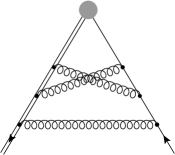
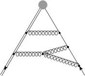
(a)	(b)	(c)
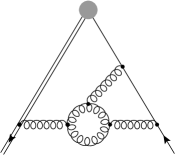
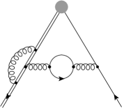
(d)	(e)	(f)
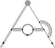
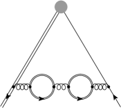
(g)	(h)	(i)

Figure 1: Sample Feynman diagrams contributing to the heavy-to-light form factors. The double solid, solid and curly lines refer to massive quarks, massless quarks and gluons, respectively. The gray blob represents one of the external currents given in Eq. (1).

One of the first steps in our calculation is the application of projectors for the scalar form factors introduced in Eq. (3). Explicit expressions are given in Appendix A. Afterwards there are no open indices and all the scalar products can be decomposed into denominator factors used to define the integral families. For this step we use an auxiliary file generated by tapir. In total we have contributions from 47 integral families. We extract the respective lists of integrals which serve as input for the integral reduction. For all external currents we generate the corresponding amplitude for general QCD gauge parameter $\xi$.

3.2 Integral reduction

In a next step, we want to reduce the list of integrals contributing to the amplitude to a smaller set of master integrals using integration-by-parts relations [128, 129, 130] and the Laporta algorithm [131]. Before performing the actual reduction for the amplitude, we reduce sample integrals with up to two dots and one scalar product for each integral family using Kira [124, 125], employing Fermat [132] as computational backend. These samples allow us to find a basis of master integrals in which the dependence on the space-time $d$ and the kinematic variable $s/m^{2}$ factorizes in the denominators of all coefficients appearing in the final reduction tables [133, 134]. We achieve this as well as an reduction of spurious poles in $\epsilon$ with an improved version of the code ImproveMasters.m [133].

With the basis chosen, we then perform the reductions of all integral families again employing Kira, this time exploiting the finite field techniques [135, 136, 137] implemented in FireFly [126, 127]. In addition to the separate reductions of all families, we run Kira to find symmetries between the master integrals and arrive at a set of $429$ master integrals at the three-loop level. We then use LiteRed [139, 140] and a subsequent reduction with Kira and FireFly to establish differential equations for the master integrals [141, 142, 143, 144] in $s/m^{2}$.

3.3 Master integrals

We calculate the master integrals at one and two loops analytically. Additionally, we also consider the master integrals which contribute to the leading-color amplitude, the ones depending on the number of light flavors, and the ones with two closed heavy-fermion loops analytically. The master integrals contributing to the leading color amplitude have been obtained before in Refs. [52, 53]. In the second reference also the leading color amplitudes for the vector, axialvector, scalar and pseudoscalar currents have been obtained. We consider in addition the tensor current. For the calculation we use the techniques of Ref. [35]. In practice this means that we do not try to find a canonical basis of master integrals, but we uncouple blocks of the differential equation into higher-order ones and solve these via the factorization of the differential operator and variation of constants. This technique is successful for the considered subset of master integrals since the differential operators factorize to first order and the results can therefore be expressed as iterated integrals over algebraic letters. We checked explicitly that this is not the case for the full amplitude, where also elliptic sectors contribute. For the implementation of the algorithms we make use of the packages Sigma [145, 146] and HarmonicSums [147, 148, 149, 150, 151, 152, 153, 154, 155, 156, 157, 158].

The boundary constants for the solution are either obtained by direct integration, Mellin-Barnes techniques, or using PSLQ [159] on numerical results computed with AMFLow [160] implementing the auxiliary-mass flow method [161, 162, 163] at the point $s=0$. Many boundary conditions can also be fixed by regularity conditions in $s/m^{2}=0$ and $s/m^{2}=1$.

We find that we can express our analytical results as iterated integrals over the alphabet

$$\frac{1}{x} \frac{1}{1\pm x} \frac{1}{2-x}~{}.$$ , ,

For the remaining master integrals we use the semi-analytic technique developed in Ref. [54, 38, 39, 40]. The method is based on series expansions around regular and singular points of the differential equation. Two neighboring expansions are then numerically matched at a point where both expansions converge. We use expansions at the points

$$\frac{s}{m^{2}} =\{-\infty,-60,-40,-30,-20,-15,-10,-8,-7,-6,-5,-4,-3,-2,-1,-1/2,$$

$$0,1/4,1/2,3/4,7/8,1\}~{},$$ (30)

where in each case we used 50 expansion terms. All but the expansions around $s/m^{2}=1$ and $s/m^{2}=-\infty$ are regular Taylor expansions. We used boundary conditions at the regular point $s/m^{2}=0$ which we obtained with the help of AMFlow demanding 100 digits precision.

4 Analytical results

As mentioned in Section 3.3, we have analytic results for all one- and two-loop form factors up to order $\epsilon^{4}$ and $\epsilon^{2}$, respectively. The computer-readable expressions for all twelve scalar form factors can be downloaded from Ref. [164] for general renormalization scales $\mu$ and $\nu$ and with the option to renormalize the scalar and pseudoscalar current in the $\overline{\rm MS}$ or in the on-shell scheme. We provide both, expressions where only the ultraviolet counterterms have been introduced, and expressions where in addition the infrared poles have been subtracted. For illustration we show in the following the result for $C_{1}^{t}$ for $\nu^{2}=\mu^{2}=m^{2}$ up to $\mathcal{O}(\epsilon^{0})$ which up to two-loop order reads ($x=s/m^{2}$):

$$C_{1}^{t,(0)} = 1\,,$$

$$C_{1}^{t,(1)} = C_{F}\biggl{\{}-\frac{3}{2}-\frac{\pi^{2}}{48}+\frac{(1-2x)H_{1}}{2x}-\frac{1}{2}H_{0,1}-H_{1,1}\biggr{\}}\,,$$

$$C_{1}^{t,(2)} = C_{A}C_{F}\biggl{\{}-\frac{119851}{20736}-\frac{\pi^{4}\big{(}-49+75x-201x^{2}+31x^{3}\big{)}}{1920(1-x)^{3}}+\frac{(354-829x)H_{1}}{216x}$$ (31)

$$+\zeta_{3}\biggl{(}\frac{398-978x+681x^{2}-137x^{3}}{576(1-x)^{3}}+\frac{7}{8}H_{1}\biggr{)}+\pi^{2}\biggl{(}\frac{253-830x-1007x^{2}}{3456(1-x)^{2}}$$

$$-\frac{\big{(}24-x+56x^{2}+65x^{3}\big{)}H_{1}}{288(1-x)^{2}x}-\frac{(2-x)\big{(}2-5x-x^{2}\big{)}H_{2}}{96(1-x)^{3}}-\frac{(1+x)(1-3x)H_{-1}}{24(1-x)x}$$

$$+\frac{\big{(}1-15x-6x^{2}-4x^{3}\big{)}H_{0,1}}{48(1-x)^{3}}+\frac{1}{24}H_{0,-1}+\frac{1}{12}H_{1,1}$$

$$-\frac{\big{(}32-48x+9x^{2}+11x^{3}\big{)}\ln(2)}{96(1-x)^{3}}\biggr{)}+\frac{\big{(}66-308x+259x^{2}-149x^{3}\big{)}H_{0,1}}{144(1-x)^{2}x}$$

$$+\frac{(2-5x)(39-83x)H_{1,1}}{144(1-x)x}+\frac{\big{(}8+12x+9x^{2}-25x^{3}\big{)}H_{0,0,1}}{48(1-x)^{3}}$$

$$-\frac{\big{(}20-192x+237x^{2}-61x^{3}\big{)}H_{0,1,1}}{48(1-x)^{3}}-\frac{\big{(}15-16x+17x^{2}\big{)}H_{1,0,1}}{16(1-x)^{2}}-\frac{11}{6}H_{1,1,1}$$

$$-\frac{(2-x)\big{(}2-5x-x^{2}\big{)}H_{2,1,1}}{48(1-x)^{3}}-\frac{(1+x)(1-3x)H_{-1,0,1}}{2(1-x)x}+\frac{\big{(}1+x+6x^{2}\big{)}H_{0,0,0,1}}{8(1-x)^{3}}$$

$$+\frac{\big{(}1+x+6x^{2}\big{)}H_{0,0,1,1}}{4(1-x)^{3}}-\frac{\big{(}1+x+6x^{2}\big{)}H_{0,1,0,1}}{8(1-x)^{3}}+\frac{1}{2}H_{0,-1,0,1}+\frac{1}{2}H_{1,0,0,1}\biggr{\}}$$

$$+C_{F}^{2}\biggl{\{}\frac{2515}{768}+\frac{\pi^{4}\big{(}389+7473x-1857x^{2}+907x^{3}\big{)}}{23040(1-x)^{3}}+H_{1,0,1,1}-\frac{(3-8x)H_{1}}{4x}$$

$$-\zeta_{3}\biggl{(}\frac{26-54x+21x^{2}+3x^{3}}{32(1-x)^{3}}+\frac{1}{2}H_{1}\biggr{)}+\pi^{2}\biggl{(}-\frac{51+47x+2x^{2}}{48(1-x)^{2}}$$

$$+\frac{\big{(}11-114x-105x^{2}+16x^{3}\big{)}H_{1}}{96(1-x)^{2}x}+\frac{(2-x)\big{(}2-5x-x^{2}\big{)}H_{2}}{48(1-x)^{3}}$$

$$+\frac{(1+x)(1-3x)H_{-1}}{12(1-x)x}-\frac{\big{(}35+135x+21x^{2}+x^{3}\big{)}H_{0,1}}{96(1-x)^{3}}-\frac{1}{12}H_{0,-1}+\frac{1}{48}H_{1,1}$$

$$+\frac{\big{(}32-48x+9x^{2}+11x^{3}\big{)}\ln(2)}{48(1-x)^{3}}\biggr{)}-\frac{\big{(}6-42x+91x^{2}+45x^{3}\big{)}H_{0,1}}{24(1-x)^{2}x}$$

$$+\frac{(97+3x)H_{1,1}}{24(1-x)}+\frac{\big{(}6+12x+84x^{2}-141x^{3}+35x^{4}\big{)}H_{0,0,1}}{24(1-x)^{3}x}-\frac{3(1-2x)H_{1,1,1}}{2x}$$

$$-\frac{\big{(}12-150x+126x^{2}-51x^{3}+59x^{4}\big{)}H_{0,1,1}}{24(1-x)^{3}x}+\frac{\big{(}-41-68x+13x^{2}\big{)}H_{1,0,1}}{24(-1+x)^{2}}$$

$$-\frac{(-2+x)\big{(}-2+5x+x^{2}\big{)}H_{2,1,1}}{24(-1+x)^{3}}+\frac{(1+x)(-1+3x)H_{-1,0,1}}{(-1+x)x}$$

$$-\frac{\big{(}1+17x-4x^{2}+2x^{3}\big{)}H_{0,0,0,1}}{4(-1+x)^{3}}-\frac{\big{(}3+11x+2x^{2}\big{)}H_{0,0,1,1}}{2(-1+x)^{3}}+\frac{1}{2}H_{1,1,0,1}+3H_{1,1,1,1}$$

$$+\frac{\big{(}2+14x-x^{2}+x^{3}\big{)}H_{0,1,0,1}}{4(-1+x)^{3}}+\frac{3}{2}H_{0,1,1,1}-H_{0,-1,0,1}-H_{1,0,0,1}\biggr{\}}$$

$$+C_{F}T_{F}n_{h}\biggl{\{}\frac{2267-5398x+4283x^{2}}{1296(-1+x)^{2}}-\frac{\pi^{2}\big{(}-11+45x-57x^{2}+7x^{3}\big{)}}{108(-1+x)^{3}}$$

$$+\frac{2\big{(}-6+13x-14x^{2}+19x^{3}\big{)}H_{1}}{27(-1+x)^{2}x}-\frac{(1+x)\big{(}-3+5x-5x^{2}+11x^{3}\big{)}H_{0,1}}{18(-1+x)^{3}x}$$

$$+\frac{1}{6}H_{0,0,1}-\frac{\zeta_{3}}{6}\biggr{\}}+C_{F}T_{F}n_{l}\biggl{\{}\frac{7859}{5184}+\frac{1}{864}\pi^{2}\big{(}109+48H_{1}\big{)}+\frac{(-12+31x)H_{1}}{27x}$$

$$-\frac{(3-11x)H_{0,1}}{18x}-\frac{(3-11x)H_{1,1}}{9x}+\frac{1}{6}H_{0,0,1}+\frac{1}{3}H_{0,1,1}+\frac{1}{3}H_{1,0,1}+\frac{2}{3}H_{1,1,1}$$

$$+\frac{13\zeta_{3}}{72}\biggr{\}}\,.$$

The one-loop order has successfully been compared to Ref. [61] up to order $\epsilon^{2}$ and has been extended to $\epsilon^{4}$. Similarly, our two-loop results up to the constant part in $\epsilon$ agrees with Ref. [61] and we have added $\epsilon^{1}$ and $\epsilon^{2}$ terms.

After multiplying $\Gamma_{\mu\nu}^{t}(q_{1},q_{2})$ in Eq. (3) with $q^{\nu}$ and projecting the result to $F_{2}^{v}$ we obtain the contribution for $b\to s\gamma$ which is given by

$$F_{1}^{t}-\frac{1}{2}F_{2}^{t}-\frac{1}{2}F_{3}^{t}\,.$$ (32)

Using our analytic results we find agreement with the numerical expressions given in Eqs. (88) and (89) of Ref. [69].

At three-loop order the amplitude can be divided up into the different color factors

$$F_{i}^{x,(3)} = C_{F}T_{F}^{2}n_{l}^{2}F_{i}^{x,(3),n_{l}^{2}}+C_{F}T_{F}^{2}n_{h}^{2}F_{i}^{x,(3),n_{h}^{2}}+C_{F}T_{F}^{2}n_{l}n_{h}F_{i}^{x,(3),n_{l}n_{h}}$$ (33)

$$+C_{F}^{2}T_{F}n_{l}F_{i}^{x,(3),C_{F}n_{l}}+C_{F}C_{A}T_{F}n_{l}F_{i}^{x,(3),C_{A}n_{l}}+N_{C}^{3}F_{i}^{x,(3),N_{C}^{3}}$$

$$+C_{F}^{2}n_{h}T_{F}F_{i}^{x,(3),C_{F}n_{h}}+C_{F}C_{A}n_{h}T_{F}F_{i}^{x,(3),C_{A}n_{h}}+\mathcal{O}\left(N_{C}^{2}\right)$$

up to color suppressed contributions. We have computed the first six terms analytically. The corresponding expressions can again be downloaded from the webpage [164]. The explicit three-loop expressions for the tensor coefficient $C_{1}^{t}$ read

$$C_{1}^{t,(3),n_{l}^{2}} = -\frac{370949}{419904}-\frac{221\pi^{4}}{38880}-\pi^{2}\biggl{(}\frac{829}{3888}-\frac{(3-11x)H_{1}}{81x}+\frac{1}{27}H_{0,1}+\frac{2}{27}H_{1,1}\biggr{)}$$ (34)

$$+\frac{(657-1430x)H_{1}}{1458x}+\frac{(48-121x)H_{0,1}}{162x}+\frac{(48-121x)H_{1,1}}{81x}$$

$$+\frac{(3-11x)H_{0,0,1}}{27x}+\frac{2(3-11x)H_{0,1,1}}{27x}+\frac{2(3-11x)H_{1,0,1}}{27x}-\frac{4}{9}H_{1,1,0,1}$$

$$+\frac{4(3-11x)H_{1,1,1}}{27x}-\frac{1}{9}H_{0,0,0,1}-\frac{2}{9}H_{0,0,1,1}-\frac{2}{9}H_{0,1,0,1}-\frac{4}{9}H_{0,1,1,1}$$

$$-\frac{2}{9}H_{1,0,0,1}-\frac{4}{9}H_{1,0,1,1}-\frac{8}{9}H_{1,1,1,1}-\frac{\big{(}323+126H_{1}\big{)}\zeta_{3}}{486}~{},$$

$$C_{1}^{t,(3),n_{h}^{2}} = -\frac{\pi^{4}}{540}+\frac{\pi^{2}(5+3x)}{135(1-x)}-\frac{667-2704x+4273x^{2}-3070x^{3}+810x^{4}}{324(1-x)^{4}}$$ (35)

$$+\zeta_{3}\biggl{(}\frac{21-162x+483x^{2}-668x^{3}+477x^{4}-198x^{5}+39x^{6}}{27(-1+x)^{6}}+\frac{2}{9}H_{1}\biggr{)}$$

$$+\frac{\big{(}438-2147x+4124x^{2}-4926x^{3}+3734x^{4}-1079x^{5}\big{)}H_{1}}{972(1-x)^{4}x}$$

$$+\frac{(1+x)\big{(}48-193x+282x^{2}-346x^{3}+354x^{4}-121x^{5}\big{)}H_{0,1}}{162(1-x)^{5}x}$$

$$+\frac{\big{(}3-11x+39x^{2}-123x^{3}+153x^{4}-75x^{5}+33x^{6}-11x^{7}\big{)}}{27(1-x)^{6}x}H_{0,0,1}$$

$$-\frac{1}{9}H_{0,0,0,1}-\frac{2}{9}H_{1,0,0,1}~{},$$

$$C_{1}^{t,(3),n_{h}n_{l}} = -\frac{\pi^{4}}{810}-\frac{23611-43766x+9787x^{2}}{5832(1-x)^{2}}+\pi^{2}\biggl{(}\frac{371-585x-327x^{2}+349x^{3}}{1944(1-x)^{3}}$$ (36)

$$-\frac{(1+x)\big{(}3-5x+5x^{2}-11x^{3}\big{)}H_{1}}{81(1-x)^{3}x}+\frac{1}{27}H_{0,1}\biggr{)}$$

$$+\frac{\big{(}73-308x+421x^{2}-138x^{3}\big{)}H_{1}}{81(1-x)^{2}x}-\frac{2}{9}H_{0,0,0,1}-\frac{2}{9}H_{0,0,1,1}$$

$$+\frac{\big{(}48-157x+153x^{2}-27x^{3}+31x^{4}\big{)}H_{0,1}}{81(1-x)^{3}x}$$

$$+\frac{8\big{(}6-13x+14x^{2}-19x^{3}\big{)}H_{1,1}}{81(1-x)^{2}x}+\frac{2\big{(}3-11x+27x^{2}-24x^{3}-11x^{4}\big{)}H_{0,0,1}}{27(1-x)^{3}x}$$

$$+\frac{2(1+x)\big{(}3-5x+5x^{2}-11x^{3}\big{)}H_{0,1,1}}{27(1-x)^{3}x}-\frac{2}{9}H_{0,1,0,1}+\frac{2\big{(}10-20x+x^{2}\big{)}\zeta_{3}}{27(1-x)^{2}}$$

$$+\frac{2(1+x)\big{(}3-5x+5x^{2}-11x^{3}\big{)}H_{1,0,1}}{27(1-x)^{3}x}~{},$$

$$C_{1}^{t,(3),C_{R}n_{l}} = -\frac{82223}{62208}+H_{0,-1,0,1,1}+\pi^{4}\biggl{(}\frac{52459+113919x-71799x^{2}+48173x^{3}}{622080(-1+x)^{3}}$$ (37)

$$+\frac{61H_{1}}{4320}\biggr{)}+\zeta_{3}\biggl{(}-\frac{6142-6438x-3345x^{2}+3155x^{3}}{2592(-1+x)^{3}}$$

$$-\frac{\big{(}-73+70x-473x^{2}+284x^{3}\big{)}H_{1}}{144(-1+x)^{2}x}+\frac{7(-2+x)\big{(}-2+5x+x^{2}\big{)}H_{2}}{144(-1+x)^{3}}$$

$$-\frac{(1+x)(-1+3x)H_{-1}}{4(-1+x)x}-\frac{\big{(}-49+387x-231x^{2}+85x^{3}\big{)}H_{0,1}}{144(-1+x)^{3}}+\frac{1}{4}H_{0,-1}$$

$$-\frac{91}{72}H_{1,1}\biggr{)}+\pi^{2}\biggl{[}\frac{575209+500974x+5545x^{2}}{248832(-1+x)^{2}}$$

$$+\ln(2)\biggl{(}\frac{280-516x+249x^{2}+5x^{3}}{144(-1+x)^{3}}+\frac{(7+17x)H_{1}}{36(-1+x)}-\frac{1}{6}H_{0,-1}+\frac{1}{6}H_{1,1}$$

$$+\frac{(-2+x)\big{(}-2+5x+x^{2}\big{)}H_{2}}{72(-1+x)^{3}}+\frac{(1+x)(-1+3x)H_{-1}}{6(-1+x)x}\biggr{)}$$

$$-\frac{\big{(}1569-14528x-11363x^{2}+2434x^{3}\big{)}H_{1}}{5184(-1+x)^{2}x}+\frac{(2-x)\big{(}26-31x+23x^{2}\big{)}H_{2}}{144(1-x)^{3}}$$

$$-\frac{(1+x)\big{(}41-131x+102x^{2}\big{)}H_{-1}}{216(-1+x)^{2}x}$$

$$-\frac{\big{(}-402+2899x+1347x^{2}-2175x^{3}+923x^{4}\big{)}H_{0,1}}{1728(-1+x)^{3}x}$$

$$-\frac{\big{(}-12+71x-117x^{2}+15x^{3}+19x^{4}\big{)}H_{0,-1}}{216(-1+x)^{3}x}$$

$$-\frac{\big{(}90-1117x-1636x^{2}+359x^{3}\big{)}H_{1,1}}{864(-1+x)^{2}x}+\frac{(6+x)H_{1,2}}{36x}$$

$$-\frac{(1+x)(-1+3x)H_{1,-1}}{18(-1+x)x}+\frac{(-2+x)\big{(}-2+5x+x^{2}\big{)}H_{2,1}}{72(-1+x)^{3}}$$

$$-\frac{(-2+x)\big{(}-2+5x+x^{2}\big{)}H_{2,2}}{72(-1+x)^{3}}+\frac{(1+x)(-1+3x)H_{-1,1}}{9(-1+x)x}$$

$$+\frac{(1+x)(-1+3x)H_{-1,-1}}{18(-1+x)x}+\frac{\big{(}-107-79x-181x^{2}+47x^{3}\big{)}H_{0,0,1}}{288(-1+x)^{3}}$$

$$+\frac{1}{18}H_{0,0,-1}-\frac{\big{(}21+97x+7x^{2}+3x^{3}\big{)}H_{0,1,1}}{48(-1+x)^{3}}-\frac{1}{6}H_{0,1,2}+\frac{1}{18}H_{0,1,-1}$$

$$-\frac{1}{9}H_{0,-1,1}-\frac{1}{18}H_{0,-1,-1}-\frac{1}{144}H_{1,0,1}-\frac{13}{72}H_{1,1,1}-\frac{1}{6}H_{1,1,2}$$

$$-\frac{\big{(}40-72x+15x^{2}+13x^{3}\big{)}\ln^{2}(2)}{108(-1+x)^{3}}$$

$$+\frac{\big{(}725+14145x-3537x^{2}+1723x^{3}\big{)}\zeta_{3}}{3456(-1+x)^{3}}\biggr{]}$$

$$-\frac{(-7103+22516x)H_{1}}{10368x}+\frac{\big{(}4608-27263x+80878x^{2}+36529x^{3}\big{)}H_{0,1}}{10368(-1+x)^{2}x}$$

$$+\frac{\big{(}-432+2976x+44615x^{2}+217x^{3}\big{)}H_{1,1}}{5184(-1+x)x^{2}}$$

$$+\frac{\big{(}14+217x+207x^{2}-730x^{3}+274x^{4}\big{)}H_{0,0,1}}{72(-1+x)^{3}x}$$

$$-\frac{\big{(}246-3392x+3372x^{2}-363x^{3}+83x^{4}\big{)}H_{0,1,1}}{216(-1+x)^{3}x}$$

$$+\frac{\big{(}-90+701x+1220x^{2}+89x^{3}\big{)}H_{1,0,1}}{216(-1+x)^{2}x}$$

$$-\frac{\big{(}18-87x+19x^{2}\big{)}H_{1,1,1}}{9(-1+x)x}+\frac{(-2+x)\big{(}26-31x+23x^{2}\big{)}H_{2,1,1}}{72(-1+x)^{3}}$$

$$-\frac{(1+x)\big{(}41-131x+102x^{2}\big{)}H_{-1,0,1}}{18(-1+x)^{2}x}$$

$$+\frac{\big{(}12+22x+338x^{2}-415x^{3}+127x^{4}\big{)}H_{0,0,0,1}}{36(-1+x)^{3}x}$$

$$-\frac{\big{(}12-285x-121x^{2}+128x^{3}+22x^{4}\big{)}H_{0,0,1,1}}{36(-1+x)^{3}x}$$

$$-\frac{\big{(}-9+34x+13x^{2}+25x^{3}+x^{4}\big{)}H_{0,1,0,1}}{18(-1+x)^{3}x}$$

$$-\frac{\big{(}21-231x+339x^{2}-270x^{3}+137x^{4}\big{)}H_{0,1,1,1}}{18(-1+x)^{3}x}$$

$$-\frac{\big{(}-12+71x-117x^{2}+15x^{3}+19x^{4}\big{)}H_{0,-1,0,1}}{18(-1+x)^{3}x}$$

$$+\frac{\big{(}-24+17x-238x^{2}+101x^{3}\big{)}H_{1,0,0,1}}{36(-1+x)^{2}x}$$

$$-\frac{\big{(}-15+140x-109x^{2}+80x^{3}\big{)}H_{1,0,1,1}}{18(-1+x)^{2}x}$$

$$-\frac{\big{(}-12-5x-254x^{2}+79x^{3}\big{)}H_{1,1,0,1}}{36(-1+x)^{2}x}-\frac{10(-1+3x)H_{1,1,1,1}}{3x}$$

$$+\frac{(6+x)H_{1,2,1,1}}{18x}-\frac{2(1+x)(-1+3x)H_{1,-1,0,1}}{3(-1+x)x}$$

$$+\frac{(-2+x)\big{(}-2+5x+x^{2}\big{)}H_{2,1,1,1}}{18(-1+x)^{3}}-\frac{(-2+x)\big{(}-2+5x+x^{2}\big{)}H_{2,2,1,1}}{36(-1+x)^{3}}$$

$$-\frac{5(1+x)(-1+3x)H_{-1,0,0,1}}{6(-1+x)x}-\frac{(1+x)(-1+3x)H_{-1,0,1,1}}{(-1+x)x}$$

$$-\frac{2(1+x)(-1+3x)H_{-1,1,0,1}}{3(-1+x)x}+\frac{2(1+x)(-1+3x)H_{-1,-1,0,1}}{3(-1+x)x}$$

$$+\frac{\big{(}1+17x-4x^{2}+2x^{3}\big{)}H_{0,0,0,0,1}}{3(-1+x)^{3}}+\frac{\big{(}5+25x+x^{2}+x^{3}\big{)}H_{0,0,0,1,1}}{3(-1+x)^{3}}$$

$$+\frac{\big{(}-4+32x-19x^{2}+7x^{3}\big{)}H_{0,0,1,0,1}}{12(-1+x)^{3}}-\frac{(1+x)\big{(}15+20x-3x^{2}\big{)}H_{0,0,1,1,1}}{6(1-x)^{3}}$$

$$+\frac{2}{3}H_{0,0,-1,0,1}+\frac{\big{(}-2+66x-27x^{2}+11x^{3}\big{)}H_{0,1,0,0,1}}{12(-1+x)^{3}}$$

$$-\frac{\big{(}-9-13x-13x^{2}+3x^{3}\big{)}H_{0,1,0,1,1}}{6(-1+x)^{3}}-\frac{\big{(}1+17x-4x^{2}+2x^{3}\big{)}H_{0,1,1,0,1}}{3(-1+x)^{3}}$$

$$-\frac{10}{3}H_{0,1,1,1,1}-\frac{1}{3}H_{0,1,2,1,1}+\frac{2}{3}H_{0,1,-1,0,1}+\frac{5}{6}H_{0,-1,0,0,1}+\frac{2}{3}H_{0,-1,1,0,1}$$

$$-\frac{2}{3}H_{0,-1,-1,0,1}+2H_{1,0,0,0,1}+\frac{2}{3}H_{1,0,1,0,1}-3H_{1,0,1,1,1}+\frac{11}{6}H_{1,1,0,0,1}$$

$$-2H_{1,1,0,1,1}-\frac{4}{3}H_{1,1,1,0,1}-\frac{20}{3}H_{1,1,1,1,1}-\frac{1}{3}H_{1,1,2,1,1}$$

$$-\frac{\big{(}68-108x+21x^{2}+23x^{3}\big{)}\ln^{4}(2)}{432(-1+x)^{3}}-\frac{\big{(}68-108x+21x^{2}+23x^{3}\big{)}\mathrm{Li}_{4}\!\left(\frac{1}{2}\right)}{18(-1+x)^{3}}$$

$$+\frac{\big{(}-13-21x-18x^{2}+4x^{3}\big{)}\zeta_{5}}{9(-1+x)^{3}}~{},$$

$$C_{1}^{t,(3),C_{A}n_{l}} = \frac{4126157}{419904}+\pi^{4}\biggl{(}-\frac{113-9573x-7707x^{2}+2935x^{3}}{155520(-1+x)^{3}}-\frac{19}{864}H_{1}\biggr{)}$$ (38)

$$+\zeta_{3}\biggl{(}\frac{-5092+21000x-29703x^{2}+13309x^{3}}{5184(-1+x)^{3}}-\frac{1}{8}H_{0,-1}+\frac{3}{8}H_{1,1}$$

$$+\frac{\big{(}-36+113x-202x^{2}+173x^{3}\big{)}H_{1}}{144(-1+x)^{2}x}-\frac{7(-2+x)\big{(}-2+5x+x^{2}\big{)}H_{2}}{288(-1+x)^{3}}$$

$$+\frac{(1+x)(-1+3x)H_{-1}}{8(-1+x)x}+\frac{\big{(}-7+17x-24x^{2}+6x^{3}\big{)}H_{0,1}}{24(-1+x)^{3}}\biggr{)}$$

$$+\pi^{2}\biggl{[}\frac{236191-273122x+373243x^{2}}{279936(-1+x)^{2}}+\ln(2)\biggl{(}-\frac{280-516x+249x^{2}+5x^{3}}{288(-1+x)^{3}}$$

$$-\frac{(7+17x)H_{1}}{72(-1+x)}-\frac{(-2+x)\big{(}-2+5x+x^{2}\big{)}H_{2}}{144(-1+x)^{3}}-\frac{(1+x)(-1+3x)H_{-1}}{12(-1+x)x}$$

$$+\frac{1}{12}H_{0,-1}-\frac{1}{12}H_{1,1}\biggr{)}+\frac{\big{(}-108+8077x-5921x^{2}+7780x^{3}\big{)}H_{1}}{7776(-1+x)^{2}x}$$

$$-\frac{(-2+x)\big{(}26-31x+23x^{2}\big{)}H_{2}}{288(-1+x)^{3}}+\frac{(1+x)\big{(}41-131x+102x^{2}\big{)}H_{-1}}{432(-1+x)^{2}x}$$

$$+\frac{\big{(}-16+4x-110x^{2}-145x^{3}+87x^{4}\big{)}H_{0,1}}{288(-1+x)^{3}x}$$

$$+\frac{\big{(}-12+71x-117x^{2}+15x^{3}+19x^{4}\big{)}H_{0,-1}}{432(-1+x)^{3}x}$$

$$+\frac{\big{(}96+71x+74x^{2}+335x^{3}\big{)}H_{1,1}}{864(-1+x)^{2}x}-\frac{(6+x)H_{1,2}}{72x}+\frac{(1+x)(-1+3x)H_{1,-1}}{36(-1+x)x}$$

$$-\frac{(-2+x)\big{(}-2+5x+x^{2}\big{)}H_{2,1}}{144(-1+x)^{3}}+\frac{(-2+x)\big{(}-2+5x+x^{2}\big{)}H_{2,2}}{144(-1+x)^{3}}$$

$$-\frac{(1+x)(-1+3x)H_{-1,1}}{18(-1+x)x}-\frac{(1+x)(-1+3x)H_{-1,-1}}{36(-1+x)x}$$

$$-\frac{\big{(}-3+29x+6x^{2}+8x^{3}\big{)}H_{0,0,1}}{144(-1+x)^{3}}-\frac{1}{36}H_{0,0,-1}+\frac{1}{12}H_{0,1,2}-\frac{1}{36}H_{0,1,-1}$$

$$-\frac{\big{(}-1+15x+6x^{2}+4x^{3}\big{)}H_{0,1,1}}{36(-1+x)^{3}}+\frac{1}{36}H_{0,-1,-1}+\frac{1}{18}H_{0,-1,1}-\frac{1}{9}H_{1,1,1}$$

$$+\frac{1}{12}H_{1,1,2}-\frac{\big{(}40-72x+15x^{2}+13x^{3}\big{)}\ln^{2}(2)}{216(1-x)^{3}}$$

$$-\frac{\big{(}53-23x+261x^{2}-19x^{3}\big{)}\zeta_{3}}{288(1-x)^{3}}\biggr{]}+\frac{(-98586+201431x)H_{1}}{23328x}$$

$$+\frac{\big{(}-2742+10661x-10999x^{2}+5906x^{3}\big{)}H_{0,1}}{1296(-1+x)^{2}x}$$

$$+\frac{\big{(}4431-14722x+13117x^{2}\big{)}H_{1,1}}{1296(-1+x)x}$$

$$+\frac{\big{(}264-968x+2619x^{2}-2079x^{3}+218x^{4}\big{)}H_{0,0,1}}{432(-1+x)^{3}x}$$

$$+\frac{\big{(}420-2539x+7119x^{2}-7008x^{3}+1954x^{4}\big{)}H_{0,1,1}}{432(-1+x)^{3}x}$$

$$+\frac{\big{(}-501+3274x-3920x^{2}+2143x^{3}\big{)}H_{1,0,1}}{432(-1+x)^{2}x}$$

$$+\frac{\big{(}393-2044x+1915x^{2}\big{)}H_{1,1,1}}{216(-1+x)x}-\frac{(-2+x)\big{(}26-31x+23x^{2}\big{)}H_{2,1,1}}{144(-1+x)^{3}}$$

$$+\frac{(1+x)\big{(}41-131x+102x^{2}\big{)}H_{-1,0,1}}{36(-1+x)^{2}x}$$

$$-\frac{\big{(}40+170x+177x^{2}-159x^{3}\big{)}H_{0,0,0,1}}{144(1-x)^{3}}+\frac{\big{(}2+163x-99x^{2}+10x^{3}\big{)}H_{0,0,1,1}}{36(-1+x)^{3}}$$

$$+\frac{\big{(}-145+325x-414x^{2}+94x^{3}\big{)}H_{0,1,0,1}}{144(-1+x)^{3}}$$

$$+\frac{\big{(}-125+651x-753x^{2}+219x^{3}\big{)}H_{0,1,1,1}}{72(-1+x)^{3}}$$

$$+\frac{\big{(}-12+71x-117x^{2}+15x^{3}+19x^{4}\big{)}H_{0,-1,0,1}}{36(-1+x)^{3}x}$$

$$-\frac{\big{(}-3+x+10x^{2}+10x^{3}\big{)}H_{1,0,0,1}}{18(-1+x)^{2}x}+\frac{\big{(}38-109x+47x^{2}\big{)}H_{1,0,1,1}}{18(-1+x)^{2}}$$

$$+\frac{\big{(}377-586x+401x^{2}\big{)}H_{1,1,0,1}}{144(-1+x)^{2}}+\frac{44}{9}H_{1,1,1,1}-\frac{(6+x)H_{1,2,1,1}}{36x}$$

$$+\frac{(1+x)(-1+3x)H_{1,-1,0,1}}{3(-1+x)x}-\frac{(-2+x)\big{(}-2+5x+x^{2}\big{)}H_{2,1,1,1}}{36(-1+x)^{3}}$$

$$+\frac{(-2+x)\big{(}-2+5x+x^{2}\big{)}H_{2,2,1,1}}{72(-1+x)^{3}}+\frac{5(1+x)(-1+3x)H_{-1,0,0,1}}{12(-1+x)x}$$

$$+\frac{(1+x)(-1+3x)H_{-1,0,1,1}}{2(-1+x)x}+\frac{(1+x)(-1+3x)H_{-1,1,0,1}}{3(-1+x)x}$$

$$-\frac{(1+x)(-1+3x)H_{-1,-1,0,1}}{3(-1+x)x}+\frac{\big{(}1+x+6x^{2}\big{)}H_{0,0,0,0,1}}{6(-1+x)^{3}}$$

$$+\frac{\big{(}1+x+6x^{2}\big{)}H_{0,0,0,1,1}}{3(-1+x)^{3}}+\frac{\big{(}1+x+6x^{2}\big{)}H_{0,0,1,0,1}}{24(-1+x)^{3}}+\frac{\big{(}1+x+6x^{2}\big{)}H_{0,0,1,1,1}}{3(-1+x)^{3}}$$

$$-\frac{1}{3}H_{0,0,-1,0,1}-\frac{\big{(}-7+9x-30x^{2}+4x^{3}\big{)}H_{0,1,0,0,1}}{24(-1+x)^{3}}+\frac{\big{(}1+x+6x^{2}\big{)}H_{0,1,0,1,1}}{6(-1+x)^{3}}$$

$$-\frac{\big{(}1+x+6x^{2}\big{)}H_{0,1,1,0,1}}{6(-1+x)^{3}}+\frac{1}{6}H_{0,1,2,1,1}-\frac{1}{3}H_{0,1,-1,0,1}-\frac{5}{12}H_{0,-1,0,0,1}$$

$$-\frac{1}{2}H_{0,-1,0,1,1}-\frac{1}{3}H_{0,-1,1,0,1}+\frac{1}{3}H_{0,-1,-1,0,1}-\frac{11}{12}H_{1,0,0,0,1}-\frac{2}{3}H_{1,0,0,1,1}$$

$$-\frac{1}{3}H_{1,0,1,0,1}-H_{1,1,0,0,1}-\frac{1}{6}H_{1,1,0,1,1}+\frac{1}{6}H_{1,1,2,1,1}$$

$$+\frac{\big{(}68-108x+21x^{2}+23x^{3}\big{)}\ln^{4}(2)}{864(-1+x)^{3}}+\frac{\big{(}68-108x+21x^{2}+23x^{3}\big{)}\mathrm{Li}_{4}\!\left(\frac{1}{2}\right)}{36(-1+x)^{3}}$$

$$-\frac{\big{(}-43+161x-105x^{2}+51x^{3}\big{)}\zeta_{5}}{48(-1+x)^{3}}~{},$$

$$C_{1}^{t,(3),N_{c}^{3}} = -\frac{155263507}{26873856}-\frac{\pi^{6}\big{(}-7514867-19812135x-18106521x^{2}+692147x^{3}\big{)}}{1672151040(-1+x)^{3}}$$ (39)

$$+\zeta_{5}\biggl{(}\frac{1199+6609x+3760x^{2}+162x^{3}}{768(-1+x)^{3}}-\frac{\big{(}-18-12x-43x^{2}+7x^{3}\big{)}H_{1}}{16(-1+x)^{3}}\biggr{)}$$

$$+\pi^{4}\biggl{(}-\frac{347993+1668009x-548373x^{2}+39943x^{3}}{4976640(-1+x)^{3}}$$

$$+\frac{\big{(}555-14839x+13219x^{2}+18643x^{3}+8342x^{4}\big{)}H_{1}}{368640(-1+x)^{3}x}$$

$$-\frac{\big{(}2691+21975x+7817x^{2}+2749x^{3}\big{)}H_{0,1}}{368640(-1+x)^{3}}$$

$$-\frac{\big{(}-3053-1209x-7431x^{2}+1325x^{3}\big{)}H_{1,1}}{184320(-1+x)^{3}}\biggr{)}$$

$$+\zeta_{3}\biggl{(}\frac{41639-91621x+51926x^{2}}{62208(-1+x)^{2}}-\frac{\big{(}570-7411x+3221x^{2}-4264x^{3}\big{)}H_{1}}{3456(1-x)^{2}x}$$

$$+\frac{\big{(}-18-703x-1779x^{2}-2751x^{3}+139x^{4}\big{)}H_{0,1}}{1152(-1+x)^{3}x}-\frac{15}{32}H_{1,1,1}$$

$$+\frac{\big{(}90+118x-479x^{2}+325x^{3}\big{)}H_{1,1}}{576(-1+x)^{2}x}+\frac{(-1+2x)(1+8x)H_{0,0,1}}{32(-1+x)^{3}}$$

$$-\frac{\big{(}-5+15x-12x^{2}+5x^{3}\big{)}H_{0,1,1}}{32(-1+x)^{3}}-\frac{\big{(}7+123x-3x^{2}+17x^{3}\big{)}H_{1,0,1}}{64(-1+x)^{3}}\biggr{)}$$

$$+\pi^{2}\biggl{[}-\frac{100078387+125792410x+60503731x^{2}}{71663616(-1+x)^{2}}-\frac{17}{128}H_{1,1,1,1}$$

$$-\zeta_{3}\biggl{(}\frac{6599+36435x+8073x^{2}+4549x^{3}}{27648(-1+x)^{3}}$$

$$+\frac{\big{(}335+147x+813x^{2}-143x^{3}\big{)}H_{1}}{4608(1-x)^{3}}\biggr{)}$$

$$-\frac{\big{(}-43983+479108x+357953x^{2}+115742x^{3}\big{)}H_{1}}{248832(-1+x)^{2}x}$$

$$+\frac{\big{(}-1028+5603x+12013x^{2}+1157x^{3}+867x^{4}\big{)}H_{0,1}}{9216(-1+x)^{3}x}$$

$$+\frac{\big{(}1569-1715x-12797x^{2}+307x^{3}\big{)}H_{1,1}}{13824(-1+x)^{2}x}$$

$$-\frac{\big{(}177+146x+2244x^{2}-1034x^{3}+27x^{4}\big{)}H_{0,0,1}}{4608(-1+x)^{3}x}$$

$$+\frac{\big{(}-270-1433x+5199x^{2}+2331x^{3}+689x^{4}\big{)}H_{0,1,1}}{4608(-1+x)^{3}x}$$

$$+\frac{\big{(}-192-295x-1719x^{2}-21x^{3}+67x^{4}\big{)}H_{1,0,1}}{4608(-1+x)^{3}x}$$

$$+\frac{\big{(}117+1106x+893x^{2}+476x^{3}\big{)}H_{1,1,1}}{2304(-1+x)^{2}x}$$

$$+\frac{\big{(}59+423x+23x^{2}+23x^{3}\big{)}H_{0,0,0,1}}{768(1-x)^{3}}$$

$$-\frac{\big{(}9+45x+7x^{2}+2x^{3}\big{)}H_{0,0,1,1}}{64(-1+x)^{3}}-\frac{\big{(}59+447x+109x^{2}+33x^{3}\big{)}H_{0,1,0,1}}{1536(-1+x)^{3}}$$

$$-\frac{\big{(}23+219x+21x^{2}+25x^{3}\big{)}H_{0,1,1,1}}{256(-1+x)^{3}}-\frac{\big{(}1+9x+x^{2}+x^{3}\big{)}H_{1,0,0,1}}{32(-1+x)^{3}}$$

$$-\frac{\big{(}19+183x+17x^{2}+21x^{3}\big{)}H_{1,0,1,1}}{384(-1+x)^{3}}-\frac{\big{(}23+219x+21x^{2}+25x^{3}\big{)}H_{1,1,0,1}}{768(-1+x)^{3}}\biggr{]}$$

$$-\frac{(-8459523+13259174x)H_{1}}{2985984x}-\frac{\big{(}7125-3574x-11219x^{2}\big{)}H_{1,1,1}}{3456(1-x)x}$$

$$-\frac{\big{(}-422544+762395x+879722x^{2}+1494251x^{3}\big{)}H_{0,1}}{331776(-1+x)^{2}x}$$

$$-\frac{\big{(}-7560+266112x+108349x^{2}+990011x^{3}\big{)}H_{1,1}}{165888(-1+x)x^{2}}$$

$$-\frac{\big{(}-4440-16709x-45452x^{2}+10171x^{3}\big{)}H_{0,0,1}}{6912(-1+x)^{2}x}$$

$$-\frac{\big{(}18+930x-8811x^{2}-8782x^{3}+2299x^{4}\big{)}H_{0,1,1}}{1152(-1+x)^{2}x^{2}}$$

$$-\frac{\big{(}54-5736x+38353x^{2}-10940x^{3}+23143x^{4}\big{)}H_{1,0,1}}{6912(-1+x)^{2}x^{2}}$$

$$-\frac{\big{(}420+3485x+13593x^{2}-9713x^{3}+1521x^{4}\big{)}H_{0,0,0,1}}{2304(-1+x)^{3}x}$$

$$+\frac{\big{(}366-1722x-4797x^{2}+1084x^{3}+416x^{4}\big{)}H_{0,0,1,1}}{576(-1+x)^{3}x}$$

$$-\frac{\big{(}450-2581x+1089x^{2}-8599x^{3}+335x^{4}\big{)}H_{0,1,0,1}}{2304(-1+x)^{3}x}$$

$$+\frac{\big{(}-1752+1163x+5102x^{2}+3191x^{3}\big{)}H_{0,1,1,1}}{1152(-1+x)^{2}x}$$

$$-\frac{\big{(}-93-934x-4054x^{2}+545x^{3}\big{)}H_{1,0,0,1}}{1152(-1+x)^{2}x}$$

$$+\frac{\big{(}-101+323x+42x^{2}+216x^{3}\big{)}H_{1,0,1,1}}{192(-1+x)^{2}x}$$

$$-\frac{\big{(}-186+227x-700x^{2}+677x^{3}\big{)}H_{1,1,0,1}}{1152(-1+x)^{2}x}+\frac{\big{(}249-98x+497x^{2}\big{)}H_{1,1,1,1}}{144(-1+x)x}$$

$$-\frac{\big{(}12+233x+1137x^{2}-400x^{3}+104x^{4}\big{)}H_{0,0,0,0,1}}{384(-1+x)^{3}x}$$

$$-\frac{\big{(}-60-163x-423x^{2}+158x^{3}+26x^{4}\big{)}H_{0,0,0,1,1}}{192(-1+x)^{3}x}$$

$$-\frac{\big{(}6+6x+570x^{2}-77x^{3}+47x^{4}\big{)}H_{0,0,1,0,1}}{192(-1+x)^{3}x}$$

$$+\frac{\big{(}15+379x-21x^{2}-622x^{3}+3x^{4}\big{)}H_{0,0,1,1,1}}{96(-1+x)^{3}x}$$

$$-\frac{\big{(}-6+79x+723x^{2}+33x^{3}+53x^{4}\big{)}H_{0,1,0,0,1}}{192(-1+x)^{3}x}$$

$$+\frac{\big{(}24+13x+375x^{2}-379x^{3}+27x^{4}\big{)}H_{0,1,0,1,1}}{192(-1+x)^{3}x}$$

$$+\frac{\big{(}-12-517x+495x^{2}-82x^{3}+122x^{4}\big{)}H_{0,1,1,0,1}}{384(-1+x)^{3}x}$$

$$+\frac{\big{(}18-133x-364x^{2}+47x^{3}\big{)}H_{0,1,1,1,1}}{48(-1+x)^{2}x}$$

$$+\frac{\big{(}9+x+3x^{2}+165x^{3}+2x^{4}\big{)}H_{1,0,0,0,1}}{192(-1+x)^{3}x}$$

$$+\frac{\big{(}18-148x+309x^{2}-90x^{3}+91x^{4}\big{)}H_{1,0,0,1,1}}{96(-1+x)^{3}x}$$

$$+\frac{\big{(}4+9x+42x^{2}+9x^{3}-4x^{4}\big{)}H_{1,0,1,0,1}}{64(1-x)^{3}x}+\frac{(1+5x)\big{(}4-10x+5x^{2}\big{)}H_{1,0,1,1,1}}{16(1-x)^{2}x}$$

$$-\frac{\big{(}6+29x+107x^{2}-16x^{3}\big{)}H_{1,1,0,0,1}}{192(1-x)^{2}x}$$

$$+\frac{\big{(}6+160x-155x^{2}+115x^{3}\big{)}H_{1,1,0,1,1}}{96(1-x)^{2}x}$$

$$+\frac{\big{(}151-14x+79x^{2}\big{)}H_{1,1,1,0,1}}{96(-1+x)^{2}}+\frac{5(9+26x)H_{1,1,1,1,1}}{48x}$$

$$-\frac{\big{(}2+24x+15x^{2}+4x^{3}\big{)}H_{0,0,0,0,0,1}}{32(-1+x)^{3}}+\frac{\big{(}7+57x-3x^{2}+5x^{3}\big{)}H_{0,0,0,0,1,1}}{16(-1+x)^{3}}$$

$$-\frac{\big{(}5+36x+2x^{2}+2x^{3}\big{)}H_{0,0,0,1,0,1}}{32(-1+x)^{3}}+\frac{\big{(}23+99x+29x^{2}+5x^{3}\big{)}H_{0,0,0,1,1,1}}{16(-1+x)^{3}}$$

$$-\frac{\big{(}1+12x+6x^{2}+2x^{3}\big{)}H_{0,0,1,0,0,1}}{32(-1+x)^{3}}+\frac{\big{(}4+33x+2x^{2}+3x^{3}\big{)}H_{0,0,1,0,1,1}}{16(-1+x)^{3}}$$

$$-\frac{\big{(}14+48x+7x^{2}\big{)}H_{0,0,1,1,0,1}}{32(-1+x)^{3}}+\frac{3(1+x)(1+2x)H_{0,0,1,1,1,1}}{2(-1+x)^{3}}$$

$$-\frac{x\big{(}3+5x+x^{2}\big{)}H_{0,1,0,0,0,1}}{32(-1+x)^{3}}-\frac{3\big{(}1+2x+3x^{2}\big{)}H_{0,1,0,0,1,1}}{16(-1+x)^{3}}$$

$$-\frac{\big{(}5+27x+15x^{2}+x^{3}\big{)}H_{0,1,0,1,0,1}}{64(-1+x)^{3}}-\frac{\big{(}-11+9x-17x^{2}+7x^{3}\big{)}H_{0,1,0,1,1,1}}{32(-1+x)^{3}}$$

$$+\frac{\big{(}2+18x-x^{2}+2x^{3}\big{)}H_{0,1,1,0,0,1}}{32(-1+x)^{3}}-\frac{\big{(}2+18x-x^{2}+2x^{3}\big{)}H_{0,1,1,0,1,1}}{16(-1+x)^{3}}$$

$$-\frac{3\big{(}3+15x+5x^{2}+x^{3}\big{)}H_{0,1,1,1,0,1}}{32(-1+x)^{3}}+\frac{\big{(}1+9x+x^{2}+x^{3}\big{)}H_{1,0,0,0,0,1}}{16(-1+x)^{3}}$$

$$+\frac{3\big{(}1+9x+x^{2}+x^{3}\big{)}H_{1,0,0,0,1,1}}{8(-1+x)^{3}}+\frac{3(1+x)(1+2x)H_{1,0,0,1,1,1}}{4(-1+x)^{3}}$$

$$+\frac{\big{(}3+15x+5x^{2}+x^{3}\big{)}H_{1,0,1,0,1,1}}{16(-1+x)^{3}}-\frac{\big{(}2+12x+3x^{2}+x^{3}\big{)}H_{1,0,1,1,0,1}}{8(-1+x)^{3}}$$

$$-\frac{3}{4}H_{1,0,1,1,1,1}+\frac{\big{(}1+9x+x^{2}+x^{3}\big{)}H_{1,1,0,0,0,1}}{16(-1+x)^{3}}+\frac{(1+x)(1+2x)H_{1,1,0,0,1,1}}{4(-1+x)^{3}}$$

$$-\frac{\big{(}3+15x+5x^{2}+x^{3}\big{)}H_{1,1,0,1,0,1}}{32(-1+x)^{3}}-\frac{9}{16}H_{1,1,0,1,1,1}-\frac{3}{8}H_{1,1,1,0,1,1}$$

$$-\frac{3}{16}H_{1,1,1,1,0,1}-\frac{15}{8}H_{1,1,1,1,1,1}-\frac{15}{16}H_{0,1,1,1,1,1}$$

$$-\frac{\big{(}10+1185x-42x^{2}+197x^{3}\big{)}\zeta_{3}^{2}}{576(-1+x)^{3}}~{},$$

where $\zeta_{i}$ denote the Riemann $\zeta$ function at integer argument $i$. Furthermore, we use the following convention for the iterated integrals:

$$H_{i,\vec{w}}(x) = \int\limits_{0}^{x}{\rm d}t\,w_{i}(t)\,H_{\vec{w}}(t)~{},$$ (40)

with the letters

$$w_{0}(t) =\frac{1}{t}~{}, w_{-1}(t) =\frac{1}{1+t}~{}, w_{1}(t) =\frac{1}{1-t}~{}, w_{2}(t) =\frac{1}{2-t}~{},$$

and we drop the argument for brevity, i.e. $H_{\vec{w}}(x)\equiv H_{\vec{w}}$. The first three letters define the harmonic polylogarithms. The forth letter can be avoided by allowing for harmonic polylogarithms evaluated at argument $1-x$.

We compared our analytic results for $F_{1}^{v}$, $F_{2}^{v}$, $F_{3}^{v}$ and $F^{s}$ to the ones attached to Ref. [53] including $\epsilon^{4}$ and $\epsilon^{2}$ terms at one and two-loop order, respectively. We found full agreement after adjusting for the different tensor basis and renormaliztion and after adapting the large-$N_{C}$ limit and setting all fermionic contributions to zero.

5 Numerical results

As mentioned in Section 3.3 we compute all master integrals using the method “expand and match”. As a result we obtain analytic expansions of the (unknown) three-loop expressions around the values $s/m^{2}$ given in Eq. (30) with high-precision numerical coefficients. Note that our approach provides generalized expansions which may contain logarithms of square roots of the expansion parameter, depending on the physical situation at the expansion point.

To illustrate the structure of our results we show in the following the first three expansion terms for $s/m^{2}\to 1$ of the $C_{F}^{3}$ colour factor of the renormalized and infrared subtracted form factor $C_{1}^{t}$. It is given by

$$C_{1}^{t,(3)}\Big{|}_{C_{F}^{3}} =3.95625$$

$$+1.23578L_{\beta}-1.02622L_{\beta}^{2}+1.06563L_{\beta}^{3}-0.37851L_{\beta}^{4}+0.0625L_{\beta}^{5}-0.0208333L_{\beta}^{6}$$

$$+\beta(8.31567+3.58274L_{\beta}-2.03938L_{\beta}^{2}-0.0683922L_{\beta}^{3}-0.4375L_{\beta}^{4}+0.125L_{\beta}^{5})$$

$$+\beta^{2}(-3.51595-19.1367L_{\beta}+4.25689L_{\beta}^{2}+1.3063L_{\beta}^{3}+0.614583L_{\beta}^{4}-0.1875L_{\beta}^{5})$$

$$+\beta^{3}(9.9209+35.8225L_{\beta}-2.05302L_{\beta}^{2}-4.15664L_{\beta}^{3}+0.194444L_{\beta}^{4}+0.125L_{\beta}^{5})$$

$$+O(\beta^{4}),$$ (41)

where $\beta=(1-m^{2}/s)/(1+m^{2}/s)$ and $L_{\beta}=\log(-2\beta)$. One observes that the expansion is logarithmically divergent in the limit $\beta\to 0$, however, it does not contain power suppressed terms like $1/\beta^{n}$, which are present in the bare amplitude. Similarly, we have a power-log expansion around $s/m^{2}=-\infty$. The expansion around the other $s/m^{2}$ values are all simple Taylor expansions.

We implement the expansions around the $s/m^{2}$ values of Eq. (30) in a Fortran program FFh2l which can be obtained from the website [55]. It is either possible to access the three-loop expressions within Fortran or via a Mathematica interface which has the same functionality. FFh2l provides results for the pole parts and finite contributions of all twelve ultraviolet renormalized form factors but also for the finite parts of the infrared subtracted form factors $C$. In the region

$$-75<s/m^{2}<15/16$$ (42)

we provide a grid by numerically evaluating our Taylor expansions and the analytic counterterms with the help of GiNaC [165, 166]. Around the singular points $s/m^{2}\to-\infty$ and $s/m^{2}=1$ we switch to dedicated power-log expansions as shown in Eq. (41). This includes expansions of the counterterms to increase stability. A more detailed description of FFh2l can be found in Appendix B.

As reference, we show in Fig. 2 the (finite) vector, scalar and tensor form factors for $\mu^{2}=m^{2}$ as a function of $s/m^{2}$ for $0<s<m^{2}$.

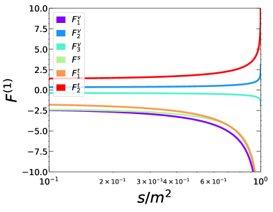
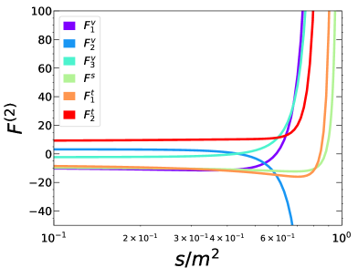
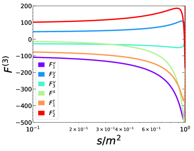
Figure 2: One-, two-, and three-loop form factors as a function of $s/m^{2}$ for $s>0$. The colour factors have been adjusted to QCD with $n_{l}=4$ and $n_{h}=1$. For the renormalization scale $\mu^{2}=m^{2}$ has been chosen.

We remind the reader that the axialvector and pseudoscalar form factors are related to the vector form factors through Eq. (6) and that $C^{t}_{3}=C^{t}_{4}=0$ as discussed in Section 2.4. For the colour factor we have chosen $C_{A}=3$, $C_{F}=4/3$ and $T_{F}=1/2$. Furthermore, we have $n_{l}=4$ and $n_{h}=1$. For the $x$ axis we have chosen a logarithmic scale since there is only a mild variation of the from factors for $s\approx 0$. On the other hand, at all loop orders we observe Coulomb-like singularities close to threshold. It is straightforward to reproduce these plots by either using the analytic one- and two-loop expressions provided as an ancillary file or with the help of the package FFh2l.

There are several checks on the correctness of our calculation. First of all, we observes that the gauge parameter cancels in the ultraviolet renormalized expressions. The analytic contributions induced by the one- and two-loop results cancel against the numerical results from the bare three-loop form factors. We observe that this cancellation happens at the level of $10^{-23}$ or significantly better which at the same time is an indication for the precision of our semi-analytic three-loop result.

An important check is the cancellation of the $1/\epsilon$ poles in the construction of $C$. As expected, there are poles up to $1/\epsilon^{6}$. All of them cancel after ultraviolet renormalization and infrared subtraction. Here, we proceed as in Refs. [39, 40] and define

$$\delta\Big{(}C^{(3)}\big{|}_{\epsilon^{i}}\Big{)}=\frac{F^{(3)}\big{|}_{\epsilon^{i}}+F^{(\text{CT}+{Z})}\big{|}_{\epsilon^{i}}}{F^{(\text{CT}+{Z})}\big{|}_{\epsilon^{i}}}\,,$$ (43)

where $F^{(3)}$ stands for the bare three-loop contribution and $F^{(\text{CT}+{Z})}$ contains the contributions induced from the analytic tree-level, one- and two-loop terms due to ultraviolet renormalization (“CT”) and infrared subtraction (“Z”). In the region given by Eq. (42), we observe that there is a cancellation of at least 16 digits for each individual colour of each form factor and each $\epsilon$ pole. Only for $s/m^{2}>15/16$ the cancellation of the grid drops below that due to the Coulomb-like singularity which supports our decision to switch to a dedicated expansion. In most parts of the phase space the cancellation is many orders of magnitude better as can be seen in Fig. 3 where we show the two worst cases of all form factors.

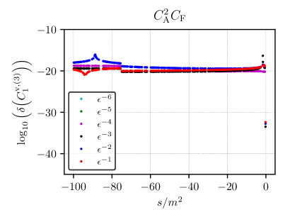
(a)	(b)
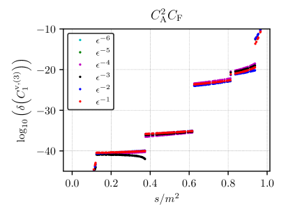
(c)	(d)

Figure 3: Relative cancellation of the poles for the the $C_{A}^{2}C_{F}$ color structures of $C_{1}^{v,(3)}$ and $C_{2}^{t,(3)}$. They show the worst behaviour of all form factors. The left panels cover the region $[-\infty,0]$ and on the right results for $0<s<1$ are shown.

Remarkably, all six orders of $\epsilon$ cancel with a similar precision. Only a careful analysis reveals a slight trend towards worse precision for the lower poles. Especially in the region $0<s/m^{2}<1$ the loss of precision when switching to the next expansion point are clearly visible, but remain on a very high level. On the negative axis, the precision curve is much smoother and only the matching from our boundary conditions at $s/m^{2}=0$ to $s/m^{2}=-1/2$ and the matching from $s/m^{2}=-60$ to $s/m^{2}\to-\infty$ stick out.

Finally, we can also check the Ward identity from Eq. (11). Naively, one would expect that it allows us to estimate the precision of the finite terms similar to the pole cancellation. However, this is not the case. It was noticed in the two-loop calculation of Ref. [43] that the Ward identity is fulfilled already on the level of the master integrals. We observe something similar: the sum of the bare three-loop contributions and the sum of the counterterm contributions to Eq. (11) are separately constant, but nonzero, and vanish when summing both contributions. This suggests that there is a similar relation between the master integrals also at the three-loop level. Since in our calculation we do not express the renormalization constants in terms of master integrals, we check Eq. (11) only numerically and observe that it is fulfilled to high precision. In most parts of the phase space it exceeds our internal precision of $50$ digits and only rarely drops below that at less stable points. Even at $s/m^{2}\approx 0.9374$, where we switch to the dedicated power-log expansion due to the Coulomb-like singularity at the threshold, the Ward identity holds to at least $19$ digits.

After all these considerations, we estimate the precision of the finite terms by extrapolating the pole cancellations and expect that our result is correct to at least $14$ digits in the grid region given by Eq. (42) and usually many more in most parts of the phase space.

For the two singular power-log expansions around $s/m^{2}\to-\infty$ and $s/m^{2}=1$ our strategy to estimate their precision differs slightly. As mentioned before, here we also expand the counterterms to increase stability. Hence, we can check the cancellation of the $1/\epsilon$ poles order by order in the expansion parameters $-m^{2}/s$ and $(1-s/m^{2})$, respectively. For the expansion around $s/m^{2}\to-\infty$, we observe that they cancel with at least $15$ digits up to order $(-m^{2}/s)^{5}$ and with at least $10$ digits up to $(-m^{2}/s)^{17}$. The expansion around $s/m^{2}=1$ behaves worse and the coefficients cancel with at least $17$ digits up to order $(1-s/m^{2})^{1}$, with at least $10$ digits up to $(1-s/m^{2})^{3}$, and with at least $9$ digits up to $(1-s/m^{2})^{20}$. Similarly, we can also check the Ward identity (11) order by order in the expansion parameters. Again we observe that it holds with high precision, reaching our internal precision of $50$ digits for most expansion orders. Hence, we conservatively estimate that the two power-log expansions in the singular regions are sufficient to provide $10$ correct digits for the finite part.

With this in mind, the grids and expansions provided in FFh2l are designed to provide at least $10$ correct digits over the full range $-\infty<s/m^{2}<1$.

6 The hard function in $\bar{B}\to X_{s}\,\gamma$

In a SCET-based approach to $\bar{B}\to X_{s}\,\gamma$ the decay width is written as the product of a hard function with a convolution of the jet and soft function [62, 63, 64]. While the latter two are known to three loops already [65, 66, 67, 68] the hard function was up to now only known to two loops [69, 70, 71]. With the three-loop matching coefficients of the tensor current at hand, we are now in the position to extract the hard function of $\bar{B}\to X_{s}\,\gamma$ to three loops as well.

To this end, we follow the discussions in Refs. [69, 70, 71] and consider the operator

$$Q_{7}=-\frac{e\,\overline{m}_{b}(\mu)}{4\pi^{2}}\,(\bar{s}_{L}\sigma_{\mu\nu}F^{\mu\nu}b_{R})\,,$$ (44)

where $\overline{m}_{b}(\mu)$ is the bottom-quark mass in the $\overline{\rm{MS}}$ scheme and $e$ the electric charge of the positron. At leading power this operator is matched onto the SCET current

$$J^{A}=(\bar{\xi}W_{hc})/\!\!\!\epsilon_{\perp}(1-\gamma_{5})h_{v}\,,$$ (45)

with the HQET field $h_{v}$ of the heavy quark, the SCET field $\xi$ of the light quark, the hard-collinear Wilson line $W_{hc}$ and the polarization vector $\epsilon_{\perp}^{\mu}$ of the on-shell photon. The field strength tensor $F^{\mu\nu}$ in Eq. (44) gives rises to the Feynman rule

$$F^{\mu\nu}=\partial^{\mu}A^{\nu}-\partial^{\nu}A^{\mu}\longrightarrow i\left(q^{\mu}\epsilon_{\perp}^{\nu}-q^{\nu}\epsilon_{\perp}^{\mu}\right)\,.$$ (46)

If the matching is done on-shell, one can use $\epsilon_{\perp}\cdot q_{2}=\epsilon_{\perp}\cdot q_{1}=0$, and arrives for $q^{2}=0$ at

$$\langle s\gamma|Q_{7}|b\rangle=-\frac{e\,\overline{m}_{b}\,2E_{\gamma}}{4\pi^{2}}\,\left(F_{1}^{t}-\frac{1}{2}\,F_{2}^{t}-\frac{1}{2}\,F_{3}^{t}\right)_{\big{|}q^{2}=0}\,\times J^{A}\,,$$ (47)

where $2E_{\gamma}\approx m_{b}$ at leading power. After infrared subtraction the expression in parenthesis becomes

$$C_{\gamma}\,\equiv\,C_{1}^{t}(s=0)-\frac{1}{2}\,C_{2}^{t}(s=0)\,.$$ (48)

The factorization formula of $\bar{B}\to X_{s}\,\gamma$ is formulated on the level of the decay rate. Moreover, since the hard function $h_{s}(\mu)$ in $\bar{B}\to X_{s}\,\gamma$ is a genuine SCET object, the logarithms of the QCD scale $\nu$ have to be set to zero in the following. We therefore arrive at

$$h_{s}(\mu) =\Big{|}{C_{\gamma}}_{\big{|}L_{\nu}=0}\Big{|}^{2}\,.$$ (49)

The explicit result of $h_{s}(\mu)$ to three loops reads

$$h_{s}(\mu) =1+C_{F}\left[-L_{\mu}^{2}-5L_{\mu}-\frac{\pi^{2}}{6}-12\right]\left(\frac{\alpha_{s}^{(n_{l})}(\mu)}{4\pi}\right)$$

$$+\left[\frac{1}{2}C_{F}^{2}L_{\mu}^{4}+L_{\mu}^{3}\left(-\frac{11}{9}C_{A}C_{F}+5C_{F}^{2}+\frac{4}{9}C_{F}n_{l}T_{F}\right)\right.$$

$$\hskip 15.0pt+\left(\left(\frac{\pi^{2}}{3}-\frac{299}{18}\right)C_{A}C_{F}+\left(\frac{49}{2}+\frac{\pi^{2}}{6}\right)C_{F}^{2}+\frac{50}{9}C_{F}n_{l}T_{F}\right)L_{\mu}^{2}$$

$$\hskip 15.0pt+\left(C_{A}C_{F}\left(22\zeta_{3}-\frac{3925}{54}-\frac{16\pi^{2}}{9}\right)+C_{F}^{2}\left(-24\zeta_{3}+\frac{117}{2}+\frac{17\pi^{2}}{6}\right)\right.$$

$$\left.\hskip 40.0pt+\left(\frac{682}{27}+\frac{8\pi^{2}}{9}\right)C_{F}n_{l}T_{F}\right)L_{\mu}+C_{F}T_{F}\left(\frac{7126}{81}-\frac{16\zeta_{3}}{3}-\frac{232\pi^{2}}{27}\right)$$

$$\hskip 15.0pt+C_{A}C_{F}\left(-\frac{122443}{648}+\frac{478\zeta_{3}}{9}+\frac{829\pi^{2}}{108}+\frac{31\pi^{4}}{60}-\frac{74}{3}\pi^{2}\ln(2)\right)$$

$$\hskip 15.0pt+C_{F}^{2}\left(\frac{3379}{24}-88\zeta_{3}-25\pi^{2}-\frac{47\pi^{4}}{72}+\frac{148}{3}\pi^{2}\ln(2)\right)$$

$$\left.\hskip 15.0pt+C_{F}n_{l}T_{F}\left(\frac{52\zeta_{3}}{9}+\frac{7859}{162}+\frac{109\pi^{2}}{27}\right)\right]\left(\frac{\alpha_{s}^{(n_{l})}(\mu)}{4\pi}\right)^{\!\!2}$$

$$+\left[-\frac{1}{6}C_{F}^{3}L_{\mu}^{6}+\left(-\frac{5}{2}C_{F}^{3}+\frac{11}{9}C_{A}C_{F}^{2}-\frac{4}{9}n_{l}T_{F}C_{F}^{2}\right)L_{\mu}^{5}+\left(-\frac{121}{54}C_{A}^{2}C_{F}-\frac{70}{9}n_{l}T_{F}C_{F}^{2}\right.\right.$$

$$\left.\hskip 40.0pt-\left(\frac{37}{2}+\frac{\pi^{2}}{12}\right)C_{F}^{3}+\left(\frac{409}{18}-\frac{\pi^{2}}{3}\right)C_{A}C_{F}^{2}-\frac{8}{27}n_{l}^{2}T_{F}^{2}C_{F}+\frac{44}{27}C_{A}n_{l}T_{F}C_{F}\right)L_{\mu}^{4}$$

$$\hskip 15.0pt+\left(\left(24\zeta_{3}-\frac{238}{3}-\frac{17\pi^{2}}{6}\right)C_{F}^{3}-\left(\frac{1540}{27}+\frac{26\pi^{2}}{27}\right)n_{l}T_{F}C_{F}^{2}-\frac{400}{81}n_{l}^{2}T_{F}^{2}C_{F}\right.$$

$$\hskip 40.0pt+\left(\frac{4601}{27}+\frac{17\pi^{2}}{54}-22\zeta_{3}\right)C_{A}C_{F}^{2}+\left(\frac{2476}{81}-\frac{8\pi^{2}}{27}\right)C_{A}n_{l}T_{F}C_{F}$$

$$\hskip 40.0pt\left.+\left(\frac{22\pi^{2}}{27}-\frac{3595}{81}\right)C_{A}^{2}C_{F}\right)L_{\mu}^{3}$$

$$\hskip 15.0pt+\left(\left(-\frac{6799}{24}+\frac{155\pi^{2}}{12}+\frac{47\pi^{4}}{72}-\frac{148}{3}\pi^{2}\ln(2)+208\zeta_{3}\right)C_{F}^{3}\right.$$

$$\hskip 40.0pt+\left(\frac{92\zeta_{3}}{9}-\frac{34205}{162}-\frac{326\pi^{2}}{27}\right)n_{l}T_{F}C_{F}^{2}+\left(\frac{16\zeta_{3}}{3}-\frac{7126}{81}+\frac{232\pi^{2}}{27}\right)T_{F}C_{F}^{2}$$

$$\hskip 40.0pt+\left(\frac{483547}{648}+\frac{395\pi^{2}}{54}-\frac{103\pi^{4}}{180}+\frac{74}{3}\pi^{2}\ln(2)-\frac{2260\zeta_{3}}{9}\right)C_{A}C_{F}^{2}$$

$$\hskip 40.0pt-\left(\frac{2680}{81}+\frac{32\pi^{2}}{27}\right)n_{l}^{2}T_{F}^{2}C_{F}+\left(\frac{220\zeta_{3}}{3}-\frac{27190}{81}-\frac{14\pi^{2}}{9}-\frac{11\pi^{4}}{45}\right)C_{A}^{2}C_{F}$$

$$\hskip 40.0pt\left.+\left(\frac{17956}{81}+\frac{112\pi^{2}}{27}-\frac{32\zeta_{3}}{3}\right)C_{A}n_{l}T_{F}C_{F}\right)L_{\mu}^{2}$$

$$\hskip 15.0pt+\left(\left(-\frac{16811}{24}+\frac{393\pi^{2}}{4}+\frac{479\pi^{4}}{360}-\frac{740}{3}\pi^{2}\ln(2)+660\zeta_{3}+\frac{28\pi^{2}\zeta_{3}}{3}+240\zeta_{5}\right)C_{F}^{3}\right.$$

$$\hskip 40.0pt+\left(\frac{1479851}{648}-\frac{29185\pi^{2}}{162}-\frac{2887\pi^{4}}{540}+\frac{4366}{9}\pi^{2}\ln(2)-\frac{13106\zeta_{3}}{9}-120\zeta_{5}\right.$$

$$\hskip 65.0pt\left.-\frac{19\pi^{2}\zeta_{3}}{3}\right)C_{A}C_{F}^{2}+\left(\frac{80\zeta_{3}}{3}-\frac{35630}{81}+\frac{1160\pi^{2}}{27}\right)T_{F}C_{F}^{2}$$

$$\hskip 40.0pt+\left(\frac{692\zeta_{3}}{3}-\frac{86683}{162}+\frac{2812\pi^{2}}{81}+\frac{16\pi^{4}}{27}-\frac{1184}{9}\pi^{2}\ln(2)\right)n_{l}T_{F}C_{F}^{2}$$

$$\hskip 40.0pt+\left(-\frac{1171918}{729}+\frac{12374\pi^{2}}{243}+\frac{107\pi^{4}}{45}-\frac{1628}{9}\pi^{2}\ln(2)+\frac{18874\zeta_{3}}{27}-100\zeta_{5}\right.$$

$$\hskip 65.0pt\left.-\frac{56\pi^{2}\zeta_{3}}{9}\right)C_{A}^{2}C_{F}-\left(\frac{83776}{729}+\frac{992\pi^{2}}{81}+\frac{448\zeta_{3}}{27}\right)n_{l}^{2}T_{F}^{2}C_{F}$$

$$\hskip 40.0pt+\left(\frac{156772}{243}-\frac{5104\pi^{2}}{81}-\frac{352\zeta_{3}}{9}\right)C_{A}T_{F}C_{F}$$

$$\hskip 40.0pt+\left(\frac{128\zeta_{3}}{9}-\frac{57008}{243}+\frac{1856\pi^{2}}{81}\right)n_{l}T_{F}^{2}C_{F}$$

$$\hskip 40.0pt\left.+\left(\frac{677290}{729}+\frac{4364\pi^{2}}{243}-\frac{8\pi^{4}}{9}+\frac{592}{9}\pi^{2}\ln(2)-\frac{1040\zeta_{3}}{9}\right)C_{A}n_{l}T_{F}C_{F}\right)L_{\mu}$$

$$\hskip 15.0pt+\left(\frac{175459\pi^{2}}{972}-\frac{219365}{486}-\frac{41303\pi^{4}}{2430}-\frac{3776}{9}\pi^{2}\ln(2)+\frac{1472}{27}\pi^{2}\ln^{2}(2)\right.$$

$$\hskip 40.0pt\left.+\frac{1072\ln^{4}(2)}{27}+\frac{8576\mathrm{Li}_{4}\!\left(\frac{1}{2}\right)}{9}+\frac{64816\zeta_{3}}{81}+\frac{298\pi^{2}\zeta_{3}}{9}+\frac{896\zeta_{5}}{9}\right)C_{F}^{2}n_{l}T_{F}$$

$$\hskip 15.0pt+\left(\frac{8584738}{6561}+\frac{151303\pi^{2}}{2187}+\frac{4703\pi^{4}}{1215}+\frac{1888}{9}\pi^{2}\ln(2)-\frac{736}{27}\pi^{2}\ln^{2}(2)-\frac{536\ln^{4}(2)}{27}\right.$$

$$\hskip 40.0pt\left.-\frac{4288\mathrm{Li}_{4}\!\left(\frac{1}{2}\right)}{9}-\frac{12640\zeta_{3}}{81}-\frac{76\pi^{2}\zeta_{3}}{9}-136\zeta_{5}\right)C_{A}C_{F}n_{l}T_{F}$$

$$\hskip 15.0pt-95.12984922305611775005\,C_{A}C_{F}T_{F}+1429.62034756690622959783\,C_{A}C_{F}^{2}$$

$$\hskip 15.0pt-3126.14625382895615802902\,C_{A}^{2}C_{F}+181.97737877492915588766\,C_{F}^{2}T_{F}$$

$$\hskip 15.0pt+345.53350842018910941336\,C_{F}^{3}+\left(\frac{128\pi^{2}}{15}-\frac{23936}{81}-\frac{32\pi^{4}}{135}+\frac{1664\zeta_{3}}{9}\right)C_{F}T_{F}^{2}$$

$$\hskip 15.0pt+\left(\frac{7088\pi^{2}}{243}-\frac{211888}{729}-\frac{64\pi^{4}}{405}+\frac{256\zeta_{3}}{27}\right)C_{F}n_{l}T_{F}^{2}$$

$$\hskip 15.0pt\left.-\left(\frac{741898}{6561}+\frac{6632\pi^{2}}{243}+\frac{884\pi^{4}}{1215}+\frac{20672\zeta_{3}}{243}\right)C_{F}n_{l}^{2}T_{F}^{2}\right]\left(\frac{\alpha_{s}^{(n_{l})}(\mu)}{4\pi}\right)^{\!\!3}+\mathcal{O}(\alpha_{s}^{4})\,.$$ (50)

In this expression, the bottom-quark mass in $L_{\mu}=\ln(\mu^{2}/m_{b}^{2})$ is renormalized in the pole scheme. In this scheme, the hard function satisfies the following RGE,

$$\frac{{\rm d}h_{s}(\mu)}{{\rm d}\ln\mu}=\biggl{[}-\gamma^{\rm cusp}(\alpha_{s}^{(n_{l})}(\mu))\ln\frac{\mu^{2}}{m_{b}^{2}}+2\gamma^{H}(\alpha_{s}^{(n_{l})}(\mu))\biggr{]}h_{s}(\mu)\,.$$ (51)

At a given order in $\alpha_{s}$, all terms containing $L_{\mu}$ are determined by the anomalous dimension coefficients and lower-loop results, and all our $L_{\mu}$ terms agree with the derivation in Ref. [71]. The $L_{\mu}$-independent terms at three loops are, however, genuinely new. In Eq. (50), all terms through to two loops are analytic and agree with Refs. [69, 70, 61, 71]. At three loops, all terms containing $L_{\mu}$, as well as the light fermionic pieces and the color factor $C_{F}T_{F}^{2}$ are also analytic. The remaining ones are obtained numerically to at least 100 decimal digits, of which we display 20 in the present write-up. An electronic version of Eq. (50) can be downloaded from the webpage [164].

Upon substituting the numerical values $C_{A}=3$, $C_{F}=4/3$, $T_{F}=1/2$, and $n_{l}=4$ for the color and flavor factors, the expansion of $h_{s}$ for $\mu=m_{b}$ reads

$$h_{s}(m_{b}) =1-4.5483113556160754788\left(\!\frac{\alpha_{s}^{(4)}(m_{b})}{\pi}\!\right)-19.286105172591724459\left(\!\frac{\alpha_{s}^{(4)}(m_{b})}{\pi}\!\right)^{\!\!2}$$

$$\hskip 22.0pt-181.16173810663548219\left(\!\frac{\alpha_{s}^{(4)}(m_{b})}{\pi}\!\right)^{\!\!3}+\mathcal{O}(\alpha_{s}^{4})\,.$$ (52)

An interesting detail to note is that the coefficient $h_{3}$, which was treated as a nuisance parameter in Ref. [71] and varied in the range $h_{3}=0\pm 80$, comes out of the genuine three-loop calculation as $h_{3}=-181.1617381$ and therefore more than a factor of two larger in magnitude compared to the variation boundaries.

7 Conclusion

We compute the three-loop QCD corrections to heavy-to-light transitions for the entire set of Dirac bilinears which are independent in four space-time dimensions. The calculations uses state-of-the art multi-loop techniques and a well-established workflow, starting from the generation of the amplitude and the projection onto Lorentz-covariant structures. The resulting scalar integrals are subsequently reduced to master integrals. A certain subset of master integrals (one- and two-loop integrals, three-loop leading color and fermionic integrals apart from the ones with a single closed heavy fermion loop) are obtained analytically, while for the others the differential equations are solved via the “expand and match” method, which uses expansions about several kinematic points and as such gives semi-analytic results for the form factors.

Infrared subtraction is applied to the ultraviolet-renormalized QCD form factors at three loops, and finite matching coefficients to SCET are obtained. In this procedure, the poles in the dimensional regulator $\epsilon$ cancel to at least $12$ digits and we thus estimate the precision of the finite part to be at least $10$ digits. From the matching coefficients of the tensor current at light-like momentum transfer, the three-loop correction to the hard function in $\bar{B}\to X_{s}\gamma$ is extracted. Further phenomenological applications to rare semileptonic decays, top-quark or muon decays are left for future investigations.

Electronic results are provided as Mathematica and Fortran codes which allow for fast and precise numerical evaluations for physically relevant values of the square of the four-momentum transfer (we do not consider values of $s/m^{2}>1$, though). The supplemenatary material to this paper can be found on the websites [164, 55, 167].

Appendix A Projectors

The scalar form factors introduced in Eq. (3) are obtained by the application of the appropriate projectors via

$$F^{\delta}_{i} = \mbox{Tr}\left[P^{\mu}_{\delta,i}\Gamma^{\delta}\right]\,,$$ (53)

where the $P^{\mu}_{\delta,i}$ are given by

$$P^{\mu}_{v,i} = \not{q}_{1}\left[g^{v}_{1,i}\gamma^{\mu}+g^{v}_{2,i}\frac{p^{\mu}}{m}+g^{v}_{3,i}\frac{q^{\mu}}{m}\right]\left(\not{q}_{2}+m\right)\,,$$

$$P^{\mu}_{a,i} = \not{q}_{1}\left[g^{a}_{1,i}\gamma^{\mu}+g^{a}_{2,i}{\frac{p^{\mu}}{m}}+g^{a}_{3,i}{\frac{q^{\mu}}{m}}\right]\gamma_{5}\left(\not{q}_{2}+m\right)\,,$$

$$P^{s} = \not{q}_{1}g_{s}\left(\not{q}_{2}+m\right)\,,$$

$$P^{p} = \not{q}_{1}{\rm{i}}g_{p}\gamma_{5}\left(\not{q}_{2}+m\right)\,,$$

$$P^{\mu\nu}_{t,j} = \not{q}_{1}\left[g^{t}_{1,j}\frac{i}{2}\sigma^{\mu\nu}+g^{t}_{2,j}\frac{q_{1}^{\mu}\gamma^{\nu}-q_{1}^{\nu}\gamma^{\mu}}{m}+g^{t}_{3,j}\frac{q_{2}^{\mu}\gamma^{\nu}-q_{2}^{\nu}\gamma^{\mu}}{m}+g^{t}_{4,j}\frac{q_{1}^{\mu}q_{2}^{\nu}-q_{1}^{\nu}q_{2}^{\mu}}{{m^{2}}}\right]\left(\not{q}_{2}+m\right),$$

with $p=q_{1}+q_{2}$, $q=q_{1}-q_{2}$, $i=1,2,3$ and $j=1,\ldots,4$. The coefficients are functions of $m$, $s$ and $\epsilon$ and read

$$g^{v}_{1,1}=\frac{s}{4(1-\epsilon)(s-m^{2})^{2}}\,, g^{v}_{2,1}=-\frac{(-3+2\epsilon)m^{2}s}{4(1-\epsilon)(s-m^{2})^{3}}\,,$$

$$g^{v}_{3,1}=-\frac{m^{2}(-2m^{2}+2\epsilon m^{2}-s)}{{4}(1-\epsilon)(s-m^{2})^{3}}\,,$$ (55)

$$g^{v}_{1,2}={-}\frac{m^{2}}{4(1-\epsilon)(s-m^{2})^{2}}\,, g^{v}_{2,2}=\frac{m^{2}(-m^{2}-2s+2\epsilon s)}{4(1-\epsilon)(s-m^{2})^{3}}\,,$$

$$g^{v}_{3,2}=\frac{(-3+2\epsilon)m^{4}}{{4}(1-\epsilon)(s-m^{2})^{3}}\,,$$ (56)

$$g^{v}_{1,3}=\frac{m^{2}}{8(1-\epsilon)(s-m^{2})^{2}}\,, g^{v}_{2,3}=-\frac{(-3+2\epsilon)m^{4}}{8(1-\epsilon)(s-m^{2})^{3}}\,,$$

$$g^{v}_{3,3}=-\frac{m^{2}(-5m^{2}+4\epsilon m^{2}+2s-2\epsilon s)}{{8}(1-\epsilon)(s-m^{2})^{3}}\,,$$ (57)

$$g^{a}_{1,1}=\frac{s}{4(1-\epsilon)(s-m^{2})^{2}}\,, g^{a}_{2,1}=\frac{(-3+2\epsilon)m^{2}s}{{4}(1-\epsilon)(s-m^{2})^{3}}\,,$$

$$g^{a}_{3,1}=\frac{m^{2}(-2m^{2}+2\epsilon m^{2}-s)}{4(1-\epsilon)(s-m^{2})^{3}}\,,$$ (58)

$$g^{a}_{1,2}=-\frac{m^{2}}{4(1-\epsilon)(s-m^{2})^{2}}\,, g^{a}_{2,2}=-\frac{m^{2}(-m^{2}-2s+2\epsilon s)}{{4}(1-\epsilon)(s-m^{2})^{3}}\,,$$

$$g^{a}_{3,2}=-\frac{(-3+2\epsilon)m^{4}}{4(1-\epsilon)(s-m^{2})^{3}}\,,$$ (59)

$$g^{a}_{1,3}=\frac{m^{2}}{{8}(1-\epsilon)(s-m^{2})^{2}}\,, g^{a}_{2,3}=\frac{(-3+2\epsilon)m^{4}}{8(1-\epsilon)(s-m^{2})^{3}}\,,$$

$$g^{a}_{3,3}=\frac{m^{2}(-5m^{2}+4\epsilon m^{2}+2s-2\epsilon s)}{{8}(1-\epsilon)(s-m^{2})^{3}}\,,$$ (60)

$$g^{s}=\frac{1}{2(m^{2}-s)}\,,$$ (61)

$$g^{p}=\frac{1}{2({m^{2}-s})}\,,$$ (62)

$$g^{t}_{1,1}=-\frac{1}{2(1-3\epsilon+2\epsilon^{2})(m^{2}-s)}\,, g^{t}_{2,1}=\frac{m^{2}}{2(-1+\epsilon)(-1+2\epsilon)(m^{2}-s)^{2}}\,,$$

$$g^{t}_{3,1}=0\,, g^{t}_{4,1}=-\frac{m^{2}}{2(1-3\epsilon+2\epsilon^{2})(m^{2}-s)^{2}}\,,$$ (63)

$$g^{t}_{1,2}=-\frac{m^{2}}{((-1+\epsilon)(-1+2\epsilon)(m^{2}-s)^{2}}\,, g^{t}_{2,2}=\frac{-(-3+2\epsilon)m^{4}}{2(-1+\epsilon)(-1+2\epsilon)(m^{2}-s)^{3}}\,,$$

$$g^{t}_{3,2}=\frac{m^{2}}{4(-1+\epsilon)(m^{2}-s)^{2}}\,, g^{t}_{4,2}=-\frac{(-3+2\epsilon)m^{4}}{2(-1+\epsilon)(-1+2\epsilon)(m^{2}-s)^{3}}\,,$$ (64)

$$g^{t}_{1,3}=0\,, g^{t}_{2,3}=\frac{m^{2}}{4(-1+\epsilon)(m^{2}-s)^{2}}\,,$$

$$g^{t}_{3,3}=0\,, g^{t}_{4,3}=0\,,$$ (65)

$$g^{t}_{1,4}=\frac{m^{2}}{(1-3\epsilon+2\epsilon^{2})(m^{2}-s)^{2}}\,, g^{t}_{2,4}=\frac{(-3+2\epsilon)m^{4}}{2(1-3\epsilon+2\epsilon^{2})(m^{2}-s)^{3}}\,,$$

$$g^{t}_{3,4}=0\,, g^{t}_{4,4}=-\frac{\epsilon(-3+2\epsilon)m^{4}}{(1-3\epsilon+2\epsilon^{2})(m^{2}-s)^{3}}\,.$$ (66)

Appendix B Implementation in computer code

In this appendix we present the implementation of the three-loop form factors for the heavy-to-light transition in the Fortran library FFh2l. The library numerically evaluates the third-order corrections to the form factors. The code is deposited on Zenodo [167] and also available at the web address

https://gitlab.com/formfactors3l/ffh2l

where documentation and sample programs can be found. The code provides interpolation grids and series expansion which can be used for instance in a Monte Carlo program.

We do not implement all series expansion presented in Eq. (30), instead we use Chebyshev interpolation grids in the range $-75<s/m^{2}<15/16$. Around the singular points $s/m^{2}=1,-\infty$ we implement the power-log expansions.

The Fortran library FFh2l can be cloned from Gitlab with

$ git clone https://gitlab.com/formfactors3l/ffh2l.git

A Fortran compiler such as gfortran is required. The library can be compiled by running

$ ./configure
make

Running make without further arguments generates the static library libffh2l.a which can be linked to the user’s program. The module files are located in the directory modules. They must be also passed to the compiler. This gives access to the public functions and subroutines. The names of all subroutines start with the suffix ffh2l_.

In order to explain the functionality of the library, let us analyze the following sample program which evaluates the vector form factor at three-loops.

program example1
  use ffh2l
  implicit none

  double complex :: ff
  double precision :: s = 0.3d0
  integer :: eporder

  print *,"EXAMPLE 1: Numerical evaluation of"
  print *,"the vector form factor F1 at s = 3/10"
  print *,"---------------------------------"
  print *,"Default configuration:"
  print *,"  - nl =4"
  print *,"  - nh =1"
  print *,""

  do eporder = -6,0
    print *,"F1( s = ",s,", ep = ",eporder," ) = ", ffh2l_veF1(s,eporder)
  enddo

  print *,""
  print *,"Form factor: finite remainder after IR subtraction"
  print *,"F1^fin( s = ",s,") = ", ffh2l_veF1_fin(s)

end program example1

In the preamble of the program, one includes use ffh2l to load the respective module. The form factor is computed by the function ffh2l_veF1(s,eporder) which returns the corresponding order in $\epsilon$ of the ultraviolet-renormalized (but not infrared subtracted) form factor $F_{1}^{v,(3)}$. The result is the third-order correction in the expansion parameter $\alpha_{s}^{(n_{l})}/(4\pi)$, the strong coupling constant renormalized in the $\overline{\mathrm{MS}}$ scheme with the renormalization scale sets to the heavy-quark mass: $\mu=m$.

For the other form factors, the user can replace veF1 in the function name with one of the following: veF2, veF3, axF1, axF2, axF3, scF1, psF1, teF1, teF2, teF3, teF4. Note that the form factors scF1 and psF1 have been implemented using as renormalization constants for the currents $Z_{s}=Z_{p}=Z^{\overline{\mathrm{MS}}}_{m}$. In addition to the 12 routines aforementioned, the user can utilize scF1OS and psF1OS to obtain results for the scalar and pseudoscalar form factors with $Z_{s}=Z_{p}=Z^{\mathrm{OS}}_{m}$ for the current renormalization.

The functions return a double complex and have the following two inputs:

double complex function ffhl2_veF1 (s,eporder)
    double precision, intent(in) :: s
    integer, intent(in) :: eporder

The variable s is the value of the momentum transfer normalized w.r.t. the squared quark mass. The order in the dimensional regulator $\epsilon=(4-d)/2$ is set by the integer eporder. Only the values eporder=-6,...,0 are valid. These form factors still contains poles since we do not perform the infrared subtraction. In this way, any infrared subtraction scheme can be applied and it is the task of the user to implement it.

For completeness, we also implement the finite remainder at three-loops after minimal subtraction of the infrared poles, as described in section 2.4. In the example above, the finite remainder for the vector form factor $F_{1}^{v,(3)}$ is obtained using the function ffh2l_veF1_fin(s). It returns the third order corrections in the expansion parameter $\alpha_{s}^{(n_{l})}/(4\pi)$. Here the strong coupling constant is renormalized in the $\overline{\mathrm{MS}}$ scheme with the renormalization scale $\mu=m$. The finite remainders for the other form factors are obtained substituting veF1 with one of the following: veF2, veF3, axF1, axF2, axF3, scF1, psF1, teF1, teF2, teF3, teF4. Also in this case, the routines with scF1 and psF1 correspond to the form factors renormalized with $Z_{s}=Z_{p}=Z^{\overline{\mathrm{MS}}}_{m}$. We provide additionally two routines identified by scF1OS and psF1OS for the finite remainder of the scalar and pseudoscalar form factors with $Z_{s}=Z_{p}=Z^{\mathrm{OS}}_{m}$.

Each function returns a double complex and has the following two inputs:

double complex function ffhl2_veF1_fin (s)
    double precision, intent(in) :: s

The variable s is the value of the momentum transfer normalized w.r.t. the squared heavy-quark mass.

In the current implementation, the numerical values of the Casimir are hard coded for QCD in the file ffh2l_global.F90. We set $C_{F}=4/3,C_{A}=3,T_{F}=1/2$. By default the number of massless and massive quarks are set to $n_{l}=4$ and $n_{h}=1$, respectively. The user can modify the values, for instance $n_{l}=3$ and $n_{h}=0$, in the following way:

integer :: nl = 3
integer :: nh = 0

call ffh2l_set_nl(nl)
call ffh2l_set_nh(nh)

In addition to the Fortran library, we provide also a Mathematica interface by making use of Wolfram’s MathLink interface (for details on the setup see Ref. [170]). The interface provides a convenient tool for numerical evaluation and cross check of our results within Mathematica. The interface is complied with

$ make mathlink

To use the library within Mathematica, the interface must be loaded:

In[] := Install["PATH/ffh2l"]

where PATH/ffh2l is the location where the mathlink executable ffh2l is saved. The ultraviolet renormalized form factors in QCD are evaluated with a call to one of the following functions:

FFh2lveF1   FFh2lveF2   FFh2lveF3
FFh2laxF1   FFh2laxF2   FFh2laxF3
FFh2lscF1   FFh2lscF1OS
FFh2lpsF1.  FFh2lpsF1OS
FFh2lteF1   FFh2lteF2   FFh2lteF3   FFh2lteF4

For instance, the order $\epsilon^{0}$ in the ultraviolet-renormalized form factor $F_{1}^{v,(3)}$ is obtained with the following command

In[] := s = 3/10;
In[] := eporder = 0;
In[] := FFh2lveF1[s,eporder]
Out[]:= 2439.87

The finite remainders of the form factors after infrared subtraction are obtained by calling the functions

FFh2lveF1Fin   FFh2lveF2Fin   FFh2lveF3Fin
FFh2laxF1Fin   FFh2laxF2Fin   FFh2laxF3Fin
FFh2lscF1Fin   FFh2lscF1OSFin
FFh2lpsF1Fin   FFh2lpsF1OSFin
FFh2lteF1Fin   FFh2lteF2Fin   FFh2lteF3Fin   FFh2lteF4Fin

For example, the finite remainder of $F_{1}^{v,(3)}$ is calculated with

In[] := s = 3/10;
In[] := FFh2lveF1Fin[s]
Out[]:= -8467.54

Also in Mathematica, it is possible to modify the default values of $n_{l}$ and $n_{h}$ in the following way:

In[] := nl=3;
In[] := nh=0;
In[] := FFh2lSetNl[nl]
In[] := FFh2lSetNh[nh]

References

- [1] G. Kramer and B. Lampe, Two-Jet Cross-Section in Annihilation, Z. Phys. C 34 (1987) 497.
- [2] T. Matsuura and W. L. van Neerven, Second order logarithmic corrections to the Drell–Yan cross-section, Z. Phys. C 38 (1988) 623.
- [3] T. Matsuura, S. C. van der Marck and W. L. van Neerven, The calculation of the second order soft and virtual contributions to the Drell-Yan cross section, Nucl. Phys. B 319 (1989) 570.
- [4] T. Gehrmann, T. Huber and D. Maître, Two-loop quark and gluon form-factors in dimensional regularisation, Phys. Lett. B 622 (2005) 295 [hep-ph/0507061].
- [5] P. A. Baikov, K. G. Chetyrkin, A. V. Smirnov, V. A. Smirnov and M. Steinhauser, Quark and Gluon Form Factors to Three Loops, Phys. Rev. Lett. 102 (2009) 212002 [0902.3519].
- [6] T. Gehrmann, E. W. N. Glover, T. Huber, N. Ikizlerli and C. Studerus, Calculation of the quark and gluon form factors to three loops in QCD, JHEP 06 (2010) 094 [1004.3653].
- [7] R. N. Lee and V. A. Smirnov, Analytic epsilon expansion of three-loop on-shell master integrals up to four-loop transcendentality weight, JHEP 02 (2011) 102 [1010.1334].
- [8] T. Gehrmann, E. W. N. Glover, T. Huber, N. Ikizlerli and C. Studerus, The quark and gluon form factors to three loops in QCD through to O, JHEP 11 (2010) 102 [1010.4478].
- [9] J. M. Henn, A. V. Smirnov, V. A. Smirnov and M. Steinhauser, A planar four-loop form factor and cusp anomalous dimension in QCD, JHEP 05 (2016) 066 [1604.03126].
- [10] A. von Manteuffel and R. M. Schabinger, Quark and gluon form factors to four-loop order in QCD: The contributions, Phys. Rev. D 95 (2017) 034030 [1611.00795].
- [11] J. Henn, R. N. Lee, A. V. Smirnov, V. A. Smirnov and M. Steinhauser, Four-loop photon quark form factor and cusp anomalous dimension in the large- limit of QCD, JHEP 03 (2017) 139 [1612.04389].
- [12] R. N. Lee, A. V. Smirnov, V. A. Smirnov and M. Steinhauser, contributions to fermionic four-loop form factors, Phys. Rev. D 96 (2017) 014008 [1705.06862].
- [13] R. N. Lee, A. V. Smirnov, V. A. Smirnov and M. Steinhauser, Four-loop quark form factor with quartic fundamental colour factor, JHEP 02 (2019) 172 [1901.02898].
- [14] A. von Manteuffel and R. M. Schabinger, Quark and gluon form factors in four loop QCD: The and contributions, Phys. Rev. D 99 (2019) 094014 [1902.08208].
- [15] A. von Manteuffel and R. M. Schabinger, Planar master integrals for four-loop form factors, JHEP 05 (2019) 073 [1903.06171].
- [16] A. von Manteuffel, E. Panzer and R. M. Schabinger, Cusp and Collinear Anomalous Dimensions in Four-Loop QCD from Form Factors, Phys. Rev. Lett. 124 (2020) 162001 [2002.04617].
- [17] R. N. Lee, A. von Manteuffel, R. M. Schabinger, A. V. Smirnov, V. A. Smirnov and M. Steinhauser, Fermionic corrections to quark and gluon form factors in four-loop QCD, Phys. Rev. D 104 (2021) 074008 [2105.11504].
- [18] R. N. Lee, A. von Manteuffel, R. M. Schabinger, A. V. Smirnov, V. A. Smirnov and M. Steinhauser, Quark and Gluon Form Factors in Four-Loop QCD, Phys. Rev. Lett. 128 (2022) 212002 [2202.04660].
- [19] A. Chakraborty, T. Huber, R. N. Lee, A. von Manteuffel, R. M. Schabinger, A. V. Smirnov et al., vertex at four loops and hard matching coefficients in SCET for various currents, Phys. Rev. D 106 (2022) 074009 [2204.02422].
- [20] R. Barbieri, J. A. Mignaco and E. Remiddi, Electron Form Factors up to Fourth Order. - I, Nuovo Cim. A 11 (1972) 824.
- [21] R. Barbieri, J. A. Mignaco and E. Remiddi, Electron Form Factors up to Fourth Order. - II, Nuovo Cim. A 11 (1972) 865.
- [22] P. Mastrolia and E. Remiddi, Two loop form-factors in QED, Nucl. Phys. B 664 (2003) 341 [hep-ph/0302162].
- [23] R. Bonciani, P. Mastrolia and E. Remiddi, QED vertex form-factors at two loops, Nucl. Phys. B 676 (2004) 399 [hep-ph/0307295].
- [24] W. Bernreuther, R. Bonciani, T. Gehrmann, R. Heinesch, T. Leineweber, P. Mastrolia et al., Two-loop QCD corrections to the heavy quark form-factors: the vector contributions, Nucl. Phys. B 706 (2005) 245 [hep-ph/0406046].
- [25] W. Bernreuther, R. Bonciani, T. Gehrmann, R. Heinesch, T. Leineweber, P. Mastrolia et al., Two-loop QCD corrections to the heavy quark form factors: Axial vector contributions, Nucl. Phys. B 712 (2005) 229 [hep-ph/0412259].
- [26] W. Bernreuther, R. Bonciani, T. Gehrmann, R. Heinesch, T. Leineweber and E. Remiddi, Two-loop QCD corrections to the heavy quark form factors: Anomaly contributions, Nucl. Phys. B 723 (2005) 91 [hep-ph/0504190].
- [27] W. Bernreuther, R. Bonciani, T. Gehrmann, R. Heinesch, P. Mastrolia and E. Remiddi, Decays of scalar and pseudoscalar Higgs bosons into fermions: Two-loop QCD corrections to the Higgs-quark-antiquark amplitude, Phys. Rev. D 72 (2005) 096002 [hep-ph/0508254].
- [28] J. Gluza, A. Mitov, S. Moch and T. Riemann, The QCD form factor of heavy quarks at NNLO, JHEP 07 (2009) 001 [0905.1137].
- [29] J. Henn, A. V. Smirnov, V. A. Smirnov and M. Steinhauser, Massive three-loop form factor in the planar limit, JHEP 01 (2017) 074 [1611.07535].
- [30] T. Ahmed, J. M. Henn and M. Steinhauser, High energy behaviour of form factors, JHEP 06 (2017) 125 [1704.07846].
- [31] J. Ablinger, A. Behring, J. Blümlein, G. Falcioni, A. De Freitas, P. Marquard et al., Heavy quark form factors at two loops, Phys. Rev. D 97 (2018) 094022 [1712.09889].
- [32] R. N. Lee, A. V. Smirnov, V. A. Smirnov and M. Steinhauser, Three-loop massive form factors: complete light-fermion corrections for the vector current, JHEP 03 (2018) 136 [1801.08151].
- [33] R. N. Lee, A. V. Smirnov, V. A. Smirnov and M. Steinhauser, Three-loop massive form factors: complete light-fermion and large-Nc corrections for vector, axial-vector, scalar and pseudo-scalar currents, JHEP 05 (2018) 187 [1804.07310].
- [34] J. Ablinger, J. Blümlein, P. Marquard, N. Rana and C. Schneider, Heavy quark form factors at three loops in the planar limit, Phys. Lett. B 782 (2018) 528 [1804.07313].
- [35] J. Ablinger, J. Blümlein, P. Marquard, N. Rana and C. Schneider, Automated solution of first order factorizable systems of differential equations in one variable, Nucl. Phys. B 939 (2019) 253 [1810.12261].
- [36] J. Blümlein, P. Marquard, N. Rana and C. Schneider, The heavy fermion contributions to the massive three loop form factors, Nucl. Phys. B 949 (2019) 114751 [1908.00357].
- [37] J. Blümlein, A. De Freitas, P. Marquard, N. Rana and C. Schneider, Analytic results on the massive three-loop form factors: Quarkonic contributions, Phys. Rev. D 108 (2023) 094003 [2307.02983].
- [38] M. Fael, F. Lange, K. Schönwald and M. Steinhauser, Massive Vector Form Factors to Three Loops, Phys. Rev. Lett. 128 (2022) 172003 [2202.05276].
- [39] M. Fael, F. Lange, K. Schönwald and M. Steinhauser, Singlet and nonsinglet three-loop massive form factors, Phys. Rev. D 106 (2022) 034029 [2207.00027].
- [40] M. Fael, F. Lange, K. Schönwald and M. Steinhauser, Massive three-loop form factors: Anomaly contribution, Phys. Rev. D 107 (2023) 094017 [2302.00693].
- [41] S. M. Berman and A. Sirlin, Some considerations on the radiative corrections to muon and neutron decay, Annals Phys. 20 (1962) 20.
- [42] C. Anastasiou, K. Melnikov and F. Petriello, The electron energy spectrum in muon decay through , JHEP 09 (2007) 014 [hep-ph/0505069].
- [43] R. Bonciani and A. Ferroglia, Two-loop QCD corrections to the heavy-to-light quark decay, JHEP 11 (2008) 065 [0809.4687].
- [44] H. M. Asatrian, C. Greub and B. D. Pecjak, Next-to-next-to-leading order corrections to in the shape-function region, Phys. Rev. D 78 (2008) 114028 [0810.0987].
- [45] M. Beneke, T. Huber and X.-Q. Li, Two-loop QCD correction to differential semi-leptonic decays in the shape-function region, Nucl. Phys. B 811 (2009) 77 [0810.1230].
- [46] G. Bell, NNLO corrections to inclusive semileptonic B decays in the shape-function region, Nucl. Phys. B 812 (2009) 264 [0810.5695].
- [47] G. Bell, Higher order QCD corrections in exclusive charmless B decays, Ph.D. thesis, Munich U., 2006. 0705.3133.
- [48] G. Bell, NNLO vertex corrections in charmless hadronic B decays: Imaginary part, Nucl. Phys. B 795 (2008) 1 [0705.3127].
- [49] T. Huber, On a two-loop crossed six-line master integral with two massive lines, JHEP 03 (2009) 024 [0901.2133].
- [50] L.-B. Chen, Two-loop master integrals for heavy-to-light form factors of two different massive fermions, JHEP 02 (2018) 066 [1801.01033].
- [51] T. Engel, C. Gnendiger, A. Signer and Y. Ulrich, Small-mass effects in heavy-to-light form factors, JHEP 02 (2019) 118 [1811.06461].
- [52] L.-B. Chen and J. Wang, Three-loop planar master integrals for heavy-to-light form factors, Phys. Lett. B 786 (2018) 453 [1810.04328].
- [53] S. Datta, N. Rana, V. Ravindran and R. Sarkar, Three loop QCD corrections to the heavy-light form factors in the color-planar limit, JHEP 12 (2023) 001 [2308.12169].
- [54] M. Fael, F. Lange, K. Schönwald and M. Steinhauser, A semi-analytic method to compute Feynman integrals applied to four-loop corrections to the -pole quark mass relation, JHEP 09 (2021) 152 [2106.05296].
- [55] https://gitlab.com/formfactors3l/ffh2l/.
- [56] C. W. Bauer, S. Fleming, D. Pirjol and I. W. Stewart, An effective field theory for collinear and soft gluons: Heavy to light decays, Phys. Rev. D 63 (2001) 114020 [hep-ph/0011336].
- [57] C. W. Bauer, D. Pirjol and I. W. Stewart, Soft-collinear factorization in effective field theory, Phys. Rev. D 65 (2002) 054022 [hep-ph/0109045].
- [58] M. Beneke, A. P. Chapovsky, M. Diehl and T. Feldmann, Soft-collinear effective theory and heavy-to-light currents beyond leading power, Nucl. Phys. B 643 (2002) 431 [hep-ph/0206152].
- [59] M. Beneke and T. Feldmann, Multipole-expanded soft-collinear effective theory with non-Abelian gauge symmetry, Phys. Lett. B 553 (2003) 267 [hep-ph/0211358].
- [60] S. W. Bosch, B. O. Lange, M. Neubert and G. Paz, Factorization and shape-function effects in inclusive -meson decays, Nucl. Phys. B 699 (2004) 335 [hep-ph/0402094].
- [61] G. Bell, M. Beneke, T. Huber and X.-Q. Li, Heavy-to-light currents at NNLO in SCET and semi-inclusive decay, Nucl. Phys. B 843 (2011) 143 [1007.3758].
- [62] G. P. Korchemsky and G. F. Sterman, Infrared factorization in inclusive B meson decays, Phys. Lett. B 340 (1994) 96 [hep-ph/9407344].
- [63] R. Akhoury and I. Z. Rothstein, Extraction of from inclusive decays and the resummation of end point logarithms, Phys. Rev. D 54 (1996) 2349 [hep-ph/9512303].
- [64] M. Neubert, Renormalization-group improved calculation of the branching ratio, Eur. Phys. J. C 40 (2005) 165 [hep-ph/0408179].
- [65] T. Becher and M. Neubert, Toward a NNLO calculation of the decay rate with a cut on photon energy: I. Two-loop result for the soft function, Phys. Lett. B 633 (2006) 739 [hep-ph/0512208].
- [66] T. Becher and M. Neubert, Toward a NNLO calculation of the decay rate with a cut on photon energy: II. Two-loop result for the jet function, Phys. Lett. B 637 (2006) 251 [hep-ph/0603140].
- [67] R. Brüser, Z. L. Liu and M. Stahlhofen, Three-Loop Quark Jet Function, Phys. Rev. Lett. 121 (2018) 072003 [1804.09722].
- [68] R. Brüser, Z. L. Liu and M. Stahlhofen, Three-loop soft function for heavy-to-light quark decays, JHEP 03 (2020) 071 [1911.04494].
- [69] A. Ali, B. D. Pecjak and C. Greub, decays at NNLO in SCET, Eur. Phys. J. C 55 (2008) 577 [0709.4422].
- [70] Z. Ligeti, I. W. Stewart and F. J. Tackmann, Treating the b quark distribution function with reliable uncertainties, Phys. Rev. D 78 (2008) 114014 [0807.1926].
- [71] B. Dehnadi, I. Novikov and F. J. Tackmann, The photon energy spectrum in B → Xs at N3LL’, JHEP 07 (2023) 214 [2211.07663].
- [72] D. R. T. Jones, Two-loop diagrams in Yang-Mills theory, Nucl. Phys. B 75 (1974) 531.
- [73] W. E. Caswell, Asymptotic Behavior of Non-Abelian Gauge Theories to Two-Loop Order, Phys. Rev. Lett. 33 (1974) 244.
- [74] E. Egorian and O. V. Tarasov, Two Loop Renormalization of the QCD in an Arbitrary Gauge, Teor. Mat. Fiz. 41 (1979) 26.
- [75] R. Tarrach, The pole mass in perturbative QCD, Nucl. Phys. B 183 (1981) 384.
- [76] N. Gray, D. J. Broadhurst, W. Grafe and K. Schilcher, Three-loop relation of quark and pole masses, Z. Phys. C 48 (1990) 673.
- [77] K. G. Chetyrkin and M. Steinhauser, Short-Distance Mass of a Heavy Quark at Order , Phys. Rev. Lett. 83 (1999) 4001 [hep-ph/9907509].
- [78] K. G. Chetyrkin and M. Steinhauser, The relation between the and the on-shell quark mass at order , Nucl. Phys. B 573 (2000) 617 [hep-ph/9911434].
- [79] K. Melnikov and T. van Ritbergen, The three-loop relation between the and the pole quark masses, Phys. Lett. B 482 (2000) 99 [hep-ph/9912391].
- [80] P. Marquard, A. V. Smirnov, V. A. Smirnov, M. Steinhauser and D. Wellmann, -on-shell quark mass relation up to four loops in QCD and a general SU gauge group, Phys. Rev. D 94 (2016) 074025 [1606.06754].
- [81] D. J. Broadhurst, N. Gray and K. Schilcher, Gauge-invariant on-shell in QED, QCD and the effective field theory of a static quark, Z. Phys. C 52 (1991) 111.
- [82] K. Melnikov and T. van Ritbergen, The three-loop on-shell renormalization of QCD and QED, Nucl. Phys. B 591 (2000) 515 [hep-ph/0005131].
- [83] P. Marquard, L. Mihaila, J. H. Piclum and M. Steinhauser, Relation between the pole and the minimally subtracted mass in dimensional regularization and dimensional reduction to three-loop order, Nucl. Phys. B 773 (2007) 1 [hep-ph/0702185].
- [84] P. Marquard, A. V. Smirnov, V. A. Smirnov and M. Steinhauser, Four-loop wave function renormalization in QCD and QED, Phys. Rev. D 97 (2018) 054032 [1801.08292].
- [85] K. G. Chetyrkin, B. A. Kniehl and M. Steinhauser, Decoupling relations to and their connection to low-energy theorems, Nucl. Phys. B 510 (1998) 61 [hep-ph/9708255].
- [86] M. Gerlach, F. Herren and M. Steinhauser, Wilson coefficients for Higgs boson production and decoupling relations to , JHEP 11 (2018) 141 [1809.06787].
- [87] O. V. Tarasov, Anomalous Dimensions of Quark Masses in the Three-Loop Approximation, Phys. Part. Nucl. Lett. 17 (2020) 109 [1910.12231].
- [88] S. A. Larin, The renormalization of the axial anomaly in dimensional regularization, Phys. Lett. B 303 (1993) 113 [hep-ph/9302240].
- [89] D. J. Broadhurst and A. G. Grozin, Matching QCD and heavy-quark effective theory heavy-light currents at two loops and beyond, Phys. Rev. D 52 (1995) 4082 [hep-ph/9410240].
- [90] J. A. Gracey, Three loop tensor current anomalous dimension in QCD, Phys. Lett. B 488 (2000) 175 [hep-ph/0007171].
- [91] S. Weinberg, Effective Gauge Theories, Phys. Lett. B 91 (1980) 51.
- [92] B. A. Ovrut and H. J. Schnitzer, Gauge Theories With Minimal Subtraction and the Decoupling Theorem, Nucl. Phys. B 179 (1981) 381.
- [93] B. A. Ovrut and H. J. Schnitzer, Gauge Theory and Effective Lagrangian, Nucl. Phys. B 189 (1981) 509.
- [94] W. Wetzel, Minimal Subtraction and the Decoupling of Heavy Quarks for Arbitrary Values of the Gauge Parameter, Nucl. Phys. B 196 (1982) 259.
- [95] W. Bernreuther and W. Wetzel, Decoupling of Heavy Quarks in the Minimal Subtraction Scheme, Nucl. Phys. B 197 (1982) 228.
- [96] W. Bernreuther, Decoupling of Heavy Quarks in Quantum Chromodynamics, Annals Phys. 151 (1983) 127.
- [97] Y. Schröder and M. Steinhauser, Four-loop decoupling relations for the strong coupling, JHEP 01 (2006) 051 [hep-ph/0512058].
- [98] K. G. Chetyrkin, J. H. Kühn and C. Sturm, QCD decoupling at four loops, Nucl. Phys. B 744 (2006) 121 [hep-ph/0512060].
- [99] A. G. Grozin, P. Marquard, J. H. Piclum and M. Steinhauser, Three-loop chromomagnetic interaction in HQET, Nucl. Phys. B 789 (2008) 277 [0707.1388].
- [100] A. G. Grozin, M. Höschele, J. Hoff and M. Steinhauser, Simultaneous decoupling of bottom and charm quarks, JHEP 09 (2011) 066 [1107.5970].
- [101] T. Becher and M. Neubert, Infrared singularities of QCD amplitudes with massive partons, Phys. Rev. D 79 (2009) 125004 [0904.1021].
- [102] Z. L. Liu and N. Schalch, Infrared Singularities of Multileg QCD Amplitudes with a Massive Parton at Three Loops, Phys. Rev. Lett. 129 (2022) 232001 [2207.02864].
- [103] S. Moch, J. A. M. Vermaseren and A. Vogt, The three-loop splitting functions in QCD: the non-singlet case, Nucl. Phys. B 688 (2004) 101 [hep-ph/0403192].
- [104] J. Davies, A. Vogt, B. Ruijl, T. Ueda and J. A. M. Vermaseren, Large- contributions to the four-loop splitting functions in QCD, Nucl. Phys. B 915 (2017) 335 [1610.07477].
- [105] S. Moch, B. Ruijl, T. Ueda, J. A. M. Vermaseren and A. Vogt, Four-loop non-singlet splitting functions in the planar limit and beyond, JHEP 10 (2017) 041 [1707.08315].
- [106] A. Grozin, Four-loop cusp anomalous dimension in QED, JHEP 06 (2018) 073 [1805.05050].
- [107] S. Moch, B. Ruijl, T. Ueda, J. A. M. Vermaseren and A. Vogt, On quartic colour factors in splitting functions and the gluon cusp anomalous dimension, Phys. Lett. B 782 (2018) 627 [1805.09638].
- [108] J. M. Henn, T. Peraro, M. Stahlhofen and P. Wasser, Matter Dependence of the Four-Loop Cusp Anomalous Dimension, Phys. Rev. Lett. 122 (2019) 201602 [1901.03693].
- [109] J. M. Henn, G. P. Korchemsky and B. Mistlberger, The full four-loop cusp anomalous dimension in super Yang-Mills and QCD, JHEP 04 (2020) 018 [1911.10174].
- [110] B. Agarwal, A. von Manteuffel, E. Panzer and R. M. Schabinger, Four-loop collinear anomalous dimensions in QCD and super Yang-Mills, Phys. Lett. B 820 (2021) 136503 [2102.09725].
- [111] S.-O. Moch, J. A. M. Vermaseren and A. Vogt, The quark form factor at higher orders, JHEP 08 (2005) 049 [hep-ph/0507039].
- [112] S. Moch, J. A. M. Vermaseren and A. Vogt, Three-loop results for quark and gluon form-factors, Phys. Lett. B 625 (2005) 245 [hep-ph/0508055].
- [113] G. P. Korchemsky and A. V. Radyushkin, Renormalization of the Wilson Loops Beyond the Leading Order, Nucl. Phys. B 283 (1987) 342.
- [114] G. P. Korchemsky and A. V. Radyushkin, Infrared factorization, Wilson lines and the heavy quark limit, Phys. Lett. B 279 (1992) 359 [hep-ph/9203222].
- [115] N. Kidonakis, Two-Loop Soft Anomalous Dimensions and Next-to-Next-to-Leading-Logarithm Resummation for Heavy Quark Production, Phys. Rev. Lett. 102 (2009) 232003 [0903.2561].
- [116] A. Grozin, J. M. Henn, G. P. Korchemsky and P. Marquard, Three Loop Cusp Anomalous Dimension in QCD, Phys. Rev. Lett. 114 (2015) 062006 [1409.0023].
- [117] A. G. Grozin, J. M. Henn, G. P. Korchemsky and P. Marquard, The three-loop cusp anomalous dimension in QCD and its supersymmetric extensions, JHEP 01 (2016) 140 [1510.07803].
- [118] P. Nogueira, Automatic Feynman Graph Generation, J. Comput. Phys. 105 (1993) 279.
- [119] M. Gerlach, F. Herren and M. Lang, tapir: A tool for topologies, amplitudes, partial fraction decomposition and input for reductions, Comput. Phys. Commun. 282 (2023) 108544 [2201.05618].
- [120] R. Harlander, T. Seidensticker and M. Steinhauser, Corrections of to the decay of the boson into bottom quarks, Phys. Lett. B 426 (1998) 125 [hep-ph/9712228].
- [121] T. Seidensticker, Automatic application of successive asymptotic expansions of Feynman diagrams, in 6th International Workshop on New Computing Techniques in Physics Research: Software Engineering, Artificial Intelligence Neural Nets, Genetic Algorithms, Symbolic Algebra, Automatic Calculation, 5, 1999, hep-ph/9905298.
- [122] J. A. M. Vermaseren, New features of FORM, math-ph/0010025.
- [123] B. Ruijl, T. Ueda and J. Vermaseren, FORM version 4.2, 1707.06453.
- [124] P. Maierhöfer, J. Usovitsch and P. Uwer, Kira—A Feynman integral reduction program, Comput. Phys. Commun. 230 (2018) 99 [1705.05610].
- [125] J. Klappert, F. Lange, P. Maierhöfer and J. Usovitsch, Integral reduction with Kira 2.0 and finite field methods, Comput. Phys. Commun. 266 (2021) 108024 [2008.06494].
- [126] J. Klappert and F. Lange, Reconstructing rational functions with FireFly, Comput. Phys. Commun. 247 (2020) 106951 [1904.00009].
- [127] J. Klappert, S. Y. Klein and F. Lange, Interpolation of dense and sparse rational functions and other improvements in FireFly, Comput. Phys. Commun. 264 (2021) 107968 [2004.01463].
- [128] F. V. Tkachov, A theorem on analytical calculability of 4-loop renormalization group functions, Phys. Lett. B 100 (1981) 65.
- [129] K. G. Chetyrkin and F. V. Tkachov, Integration by parts: The algorithm to calculate -functions in 4 loops, Nucl. Phys. B 192 (1981) 159.
- [130] T. Gehrmann and E. Remiddi, Differential equations for two-loop four-point functions, Nucl. Phys. B 580 (2000) 485 [hep-ph/9912329].
- [131] S. Laporta, High-precision calculation of multiloop Feynman integrals by difference equations, Int. J. Mod. Phys. A 15 (2000) 5087 [hep-ph/0102033].
- [132] R. Lewis, FERMAT, https://home.bway.net/lewis .
- [133] A. V. Smirnov and V. A. Smirnov, How to choose master integrals, Nucl. Phys. B 960 (2020) 115213 [2002.08042].
- [134] J. Usovitsch, Factorization of denominators in integration-by-parts reductions, 2002.08173.
- [135] M. Kauers, Fast Solvers for Dense Linear Systems, Nucl. Phys. B Proc. Suppl. 183 (2008) 245.
- [136] A. von Manteuffel and R. M. Schabinger, A novel approach to integration by parts reduction, Phys. Lett. B 744 (2015) 101 [1406.4513].
- [137] T. Peraro, Scattering amplitudes over finite fields and multivariate functional reconstruction, JHEP 12 (2016) 030 [1608.01902].
- [138] M. Driesse, G. U. Jakobsen, G. Mogull, J. Plefka, B. Sauer and J. Usovitsch, Conservative Black Hole Scattering at Fifth Post-Minkowskian and First Self-Force Order, 2403.07781.
- [139] R. N. Lee, Presenting LiteRed: a tool for the Loop InTEgrals REDuction, 1212.2685.
- [140] R. N. Lee, LiteRed 1.4: a powerful tool for reduction of multiloop integrals, J. Phys. Conf. Ser. 523 (2014) 012059 [1310.1145].
- [141] A. V. Kotikov, Differential equations method. New technique for massive Feynman diagram calculation, Phys. Lett. B 254 (1991) 158.
- [142] A. V. Kotikov, Differential equations method: the calculation of vertex-type Feynman diagrams, Phys. Lett. B 259 (1991) 314.
- [143] A. V. Kotikov, Differential equation method. The calculation of -point Feynman diagrams, Phys. Lett. B 267 (1991) 123.
- [144] E. Remiddi, Differential equations for Feynman graph amplitudes, Nuovo Cim. A 110 (1997) 1435 [hep-th/9711188].
- [145] C. Schneider, Symbolic summation assists combinatorics, Seminaire Lotharingien de Combinatoire 56 (2007) 1.
- [146] C. Schneider, Term Algebras, Canonical Representations and Difference Ring Theory for Symbolic Summation, pp. 423–485. Springer International Publishing, Cham, 2021. 2102.01471. DOI: 10.1007/978-3-030-80219-6_17.
- [147] J. Blümlein and S. Kurth, Harmonic sums and Mellin transforms up to two-loop order, Phys. Rev. D 60 (1999) 014018 [hep-ph/9810241].
- [148] J. A. M. Vermaseren, Harmonic sums, Mellin transforms and integrals, Int. J. Mod. Phys. A 14 (1999) 2037 [hep-ph/9806280].
- [149] J. Blümlein, Structural relations of harmonic sums and Mellin transforms up to weight , Comput. Phys. Commun. 180 (2009) 2218 [0901.3106].
- [150] J. Ablinger, A Computer Algebra Toolbox for Harmonic Sums Related to Particle Physics, Master’s thesis, Linz U., 2009.
- [151] J. Ablinger, J. Blümlein and C. Schneider, Harmonic sums and polylogarithms generated by cyclotomic polynomials, J. Math. Phys. 52 (2011) 102301 [1105.6063].
- [152] J. Ablinger, Computer Algebra Algorithms for Special Functions in Particle Physics, Ph.D. thesis, Linz U., 4, 2012. 1305.0687.
- [153] J. Ablinger, J. Blümlein and C. Schneider, Generalized Harmonic, Cyclotomic, and Binomial Sums, their Polylogarithms and Special Numbers, J. Phys. Conf. Ser. 523 (2014) 012060 [1310.5645].
- [154] J. Ablinger, J. Blümlein and C. Schneider, Analytic and algorithmic aspects of generalized harmonic sums and polylogarithms, J. Math. Phys. 54 (2013) 082301 [1302.0378].
- [155] J. Ablinger, J. Blümlein, C. G. Raab and C. Schneider, Iterated binomial sums and their associated iterated integrals, J. Math. Phys. 55 (2014) 112301 [1407.1822].
- [156] J. Ablinger, The package HarmonicSums: Computer Algebra and Analytic aspects of Nested Sums, PoS LL2014 (2014) 019 [1407.6180].
- [157] J. Ablinger, Discovering and Proving Infinite Binomial Sums Identities, Exper. Math. 26 (2016) 62 [1507.01703].
- [158] J. Ablinger, Computing the Inverse Mellin Transform of Holonomic Sequences using Kovacic’s Algorithm, PoS RADCOR2017 (2018) 001 [1801.01039].
- [159] H. Ferguson and D. Bailey, A Polynomial Time, Numerically Stable Integer Relation Algorithm, RNR Technical Report, RNR-91-032 .
- [160] X. Liu and Y.-Q. Ma, AMFlow: A Mathematica package for Feynman integrals computation via auxiliary mass flow, Comput. Phys. Commun. 283 (2023) 108565 [2201.11669].
- [161] X. Liu, Y.-Q. Ma and C.-Y. Wang, A systematic and efficient method to compute multi-loop master integrals, Phys. Lett. B 779 (2018) 353 [1711.09572].
- [162] X. Liu and Y.-Q. Ma, Multiloop corrections for collider processes using auxiliary mass flow, Phys. Rev. D 105 (2022) L051503 [2107.01864].
- [163] Z.-F. Liu and Y.-Q. Ma, Determining Feynman Integrals with Only Input from Linear Algebra, Phys. Rev. Lett. 129 (2022) 222001 [2201.11637].
- [164] https://www.ttp.kit.edu/preprints/2024/ttp24-017/.
- [165] C. Bauer, A. Frink and R. Kreckel, Introduction to the GiNaC Framework for Symbolic Computation within the C++ Programming Language, J. Symb. Comput. 33 (2002) 1 [cs/0004015].
- [166] J. Vollinga and S. Weinzierl, Numerical evaluation of multiple polylogarithms, Comput. Phys. Commun. 167 (2005) 177 [hep-ph/0410259].
- [167] M. Fael, T. Huber, F. Lange, J. Müller, K. Schönwald and M. Steinhauser, “Supplementary material for Heavy-to-light form factors to three loops.” URL: https://doi.org/10.5281/zenodo.11046426, 2024.
- [168] J. A. M. Vermaseren, Axodraw, Comput. Phys. Commun. 83 (1994) 45.
- [169] D. Binosi and L. Theußl, JaxoDraw: A graphical user interface for drawing Feynman diagrams, Comput. Phys. Commun. 161 (2004) 76 [hep-ph/0309015].
- [170] T. Hahn, The high-energy physicist’s guide to MathLink, Comput. Phys. Commun. 183 (2012) 460 [1107.4379].