Revisiting N₂ with Neural-Network-Supported CI

Abstract

We apply a recently proposed computational protocol for a neural-network-supported configuration interaction (NN CI) calculation to the paradigmatic N₂ molecule. By comparison of correlation energy, binding energy, and the full dissociation curve to experimental and full CI benchmarks, we demonstrate the applicability and robustness of our approach for the first time in the context of molecular systems, and offer thereby a new complementary tool in the family of machine-learning-based computation methods. The main advantage of the method lies in the efficiency of the neural-network-selected many-body basis set. Specifically, we approximate full CI results obtained on bases of $\approx 10^{10}$ Slater Determinants with only $\approx 10^{5}$ determinants with good accuracy. The high efficiency of the NN CI approach underlines its potential for broader applications such as structural optimizations and even computation of spectroscopic observables in systems for which computational resources are a limiting factor.

I Introduction

The accurate determination of the electronic ground state of molecular systems presents a critical challenge in quantum chemistry, primarily due to the exponential growth of the Hilbert space with the number of electrons and orbitals involved. For diatomic molecules such as, e.g., nitrogen N₂, obtaining precise ground state energies is particularly crucial for understanding bonding characteristics, molecular behavior under different conditions, and potential reaction pathways. Full Configuration interaction (fCI) methods belong to the most direct approaches to solve the electronic Schrödinger equation. In fCI the electronic wave function is expressed as a linear combination of basis vectors (e.g. Slater Determinants (SDets)). Determining the eigenvectors of the many-body Hamiltonian on such a basis allows, in principle, for arbitrarily exact treatment of electronic correlations[1].

However, practical application of fCI is limited by the ”exponential wall”, i.e. the combinatorial explosion of basis SDets with increasing system size. For N₂, even modest basis sets can yield an intractably large number of determinants, pushing traditional computational approaches to their limits [2]. One strategy to circumvent the basis set explosion is the so-called embedding technique. Here, the large system is subdivided into a smaller strongly correlated part (quantum cluster) which is treated with fCI accuracy, and the rest treated at a more approximate, mean-field level using Hartree–Fock[1] or Kohn–Sham density functional theory [3, 4]. Examples in quantum chemistry are embedded correlated wave function schemes and embedding potential schemes [5, 6]. While traditional and newly developed embedding techniques show great potential, the size of the embedded quantum cluster can still be the prohibiting factor for capturing essential quantum mechanical correlations. To this end, based on the observation that only a small subset of the configurations contributes significantly to the description of the eigenfunctions [7], a large variety of selected CI methods have been developed, see for example Refs. [8, 9, 10, 11] and references therein.

The advent of machine learning (ML) algorithms has given a new twist to these efforts. ML techniques have been applied in the context of selective CI computations and already shown great potential [12, 13, 14, 15, 16]. These works included calculations of explicit expansion coefficients with the help of a regression neural network (NN) [12, 17] and schemes which leverage a NN classifier to distinguish ”important” from ”unimportant” configurations without actually predicting their coefficients [13]. Related approaches have been developed recently also for the structure and dynamics of light nuclei [18], for accurate atomic structure calculations [19], and most recently in the context of effective models in strongly correlated solids [20].

In the present work, we employ the last, most recently proposed scheme of Bilous et al. [20], to the nitrogen molecule N₂ and the computation of its ground state. Our classifier consists of a convolutional neural network which performs the selection of cadidate SDets in an iterative extension procedure of the many-body Hilbert space. Our results on the correlation energy, binding energy, and the fully computed dissociation curve of N₂ show that the approach indeed works very well also for molecular structures with much more complex interactions than in the single site impurity model considered in Ref. [20].

II Methods

For the computation of the many-body wave function of a molecule we can cast the problem into a Hamiltonian form and write

$$H=H^{0}+H^{\mathrm{int}}-\mathrm{MF}\left[H^{\mathrm{int}}\right]$$ (1)

with

$$H^{0} =\sum_{i,j,\sigma}t_{ij}c^{\dagger}_{i,\sigma}c_{j,\sigma}$$ (2)

$$H^{\mathrm{int}} =\sum_{\begin{subarray}{c}i,j,k,l\\ \sigma,\sigma^{\prime}\end{subarray}}U_{ijkl}\;\;c^{\dagger}_{i,\sigma}c_{j,\sigma}c^{\dagger}_{k,\sigma^{\prime}}c_{l,\sigma^{\prime}}$$ (3)

where $c^{\dagger}_{i,\sigma}$ and $c_{i,\sigma}$ are fermionic (creation/annihilation) field operators with orbital and spin indices $i$ and $\sigma$, respectively. $t_{ij}$ and $U_{ijkl}$ are the single- and two particle integrals

$$t_{ij} \equiv\int\text{d}\mathbf{r}\varphi^{*}_{i}(\mathbf{r})\left(-\frac{1}{2}\nabla^{2}+V^{\text{eff}}(\mathbf{r})\right)\varphi_{j}(\mathbf{r})$$ (5)

$$U_{ijkl} \equiv\int\text{d}\mathbf{r}\,\text{d}\mathbf{r^{\prime}}\varphi^{*}_{i}(\mathbf{r})\varphi^{*}_{j}(\mathbf{r})\frac{1}{|\mathbf{r}-\mathbf{r^{\prime}}|}\varphi_{k}(\mathbf{r^{\prime}})\varphi_{l}(\mathbf{r^{\prime}})$$ (6)

where $V_{\text{eff}}(\mathbf{r})$ is the self-consistent mean-field potential, and the integrals are evaluated on the Hartree-Fock eigenbasis $\varphi_{i}(\mathbf{r})$. The term $\mathrm{MF}\left[H^{\mathrm{int}}\right]$ in Eq. (1) , is the mean-field decoupled interaction operator. Since its contributions are implicitly included in the Hartree-Fock single particle integrals $t_{ij}$ we need to substract it to avoid double counting.

We calculate the ground state of $H$ in two steps. In the first step we calculate the integrals $t_{ij}$ and $U_{ijkl}$. In the second step we find the ground state of $H$ on a selected many-body basis using our NN-based algorithm. All calculations in this work are performed retaining spin symmetry.

II.1 Hartree-Fock

The single- and two-particle integrals, $t_{ij}$ and $U_{ijkl}$ are calculated using the canonical orbitals obtained in Hartree-Fock calculations. In these calculations, the projector augmented wave (PAW) method [21, 22] is used to treat the electrons near the nuclei, and core electrons for each atom are frozen to the result of a reference scalar relativistic calculation of the isolated atom. Smooth pseudo wave functions for the valence electrons are described using a plane-wave basis set. Since virtual orbitals do not impact the Hartree-Fock energy, they are not explicitly optimized but taken from an auxiliary set of numerical atomic orbitals centered at the positions of the nuclei [23]. This set contains four sets of valence atomic orbitals and two sets of polarization functions, amounting to a total of four numerical $s$ and two sets of numerical $p$ orbitals for the hydrogen atom, and four numerical $s$, four sets of numerical $p$, and two sets of numerical $d$ orbitals for the nitrogen atom. For the latter, the $1s$ orbital is frozen and the total number of molecular orbitals is 52. Smaller numbers of orbitals are generated by omitting the highest-energy molecular orbitals. The Hartree-Fock calculations are carried out using a direct minimization approach [24, 25] employing the L-BFGS algorithm. The calculations are considered converged when the squared residual of the Hartree-Fock equations is below 10${}^{-11}\,\text{eV}^{2}$ per valence electron for the optimal orbitals that minimize the Hartree-Fock energy. All Hartree-Fock calculations are performed using the GPAW software [26] with a grid spacing of $0.18$ Åand the plane wave energy $1000$ eV. The sizes of the simulation cells for the H₂ benchmark and N₂ molecules are $25\times 25\times 28.34\,\text{\AA}^{3}$ and $25\times 25\times 28\,\text{\AA}^{3}$, respectively. Further details on the Hartree-Fock calculations are provided in appendices VI.1.1 and VI.1.2.

II.2 NN-suppoted CI

For the machine learning (ML) part of our calculation, we follow the recently proposed computation protocol [20] that employs the active learning (AL) technique. ML approaches are typically categorized into supervised, unsupervised, and reinforcement learning paradigms [27]. AL, however, does not strictly fall into any of these categories: While our NN classifier is trained in a supervised manner, the data for the training is not predetermined (as in the standard supervised learning paradigm) but dynamically generated during interactions with the “environment”. This process involves making decisions based on the outcomes of prior training iterations, a strategy shared with reinforcement learning, though AL lacks an explicit reward system. Instead, we focus on monitoring an observable — specifically, the ground state energy. Other observables could be also used as a convergence criterion for the iterations of the NN-supported CI algorithm.

In the CI framework, the exact solution

$$H\ket{\Psi^{\text{ex}}_{\text{gs}}}=E^{\text{ex}}_{\text{gs}}\ket{\Psi^{\text{ex}}_{\text{gs}}}$$ (7)

for the system Hamiltonian (1) is expanded in SDets $\ket{\phi}$ which form an orthonormal basis of the full Hilbert space ${\cal H}^{\text{full}}=\text{span}\left(\{\phi\}\right)$. The expansion reads

$$\ket{\Psi^{\text{ex}}_{\text{gs}}}=\sum^{N}_{\alpha}c_{\alpha}\ket{\phi_{\alpha}}\,,$$ (8)

with $N\equiv\text{dim}\left({\cal H}^{\text{full}}\right)$. We aim to approximate the exact ground state $\ket{\Psi_{\text{gs}}}$ by searching for the most relevant subspace of ${\cal H}^{s}\subset{\cal H}^{\text{full}}$ with $\text{dim}\left({\cal H}^{s}\right)=N^{s}\ll N$ for the calculation of the ground state $\ket{\Psi_{\text{gs}}}$ and its energy $E_{\text{gs}}$. The approximate wave function can be written as

$$\ket{\Psi^{\text{ex}}_{\text{gs}}}\approx\ket{\Psi_{\text{gs}}}=\sum^{N^{s}\ll N}_{\alpha}c_{\alpha}\ket{\phi_{\alpha}}.$$ (9)

The iterative procedure that converges to the approximation (9) starts from an initial basis $\{\phi^{\text{init}}\}$. The basis is iteratively extended using an extension operator $\hat{\cal O}$. In each iteration, the eigenproblem for (1) is solved yielding the approximative wave function and the ground state energy. Since the basis quickly becomes large and computationally infeasible, the NN-supported algorithm described in detail in Ref. [20] selects only the most important SDets prior to the eigenproblem solution in each iteration. For the calculations presented in this paper we set $\{\phi^{\text{init}}\}=\{\ket{\phi^{\text{HF}}_{\text{gs}}}\}$ to the (single SDet) Hartree Fock ground state expanded with the full Hamiltonian (1), i.e. $\hat{\cal O}=H$ including the full (high dimensional) $U_{ijkl}$ tensor. We followed Refs. [20, 19] and employed a NN classifier of the convolutional type [28] shown schematically in Fig. 1. The parts of the convolutional block (A)—(D) and the dense block (E)—(F), as well as other NN-related and implementation details are presented in Appendix VI.2.

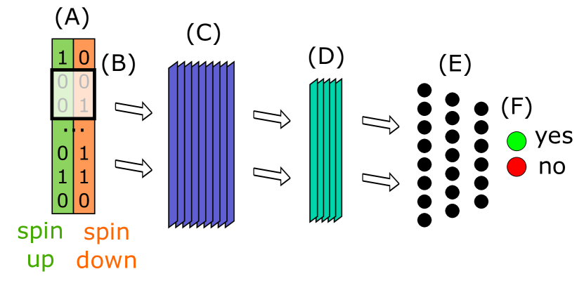
Figure 1: Architecture of the convolutional NN used in this work. A candidate SDet is given as input (A) and eventually classified as important or unimportant (F). See text for further explanations.

III Results

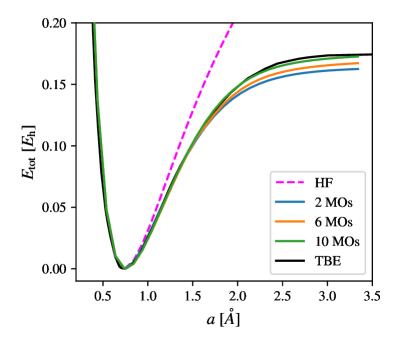
Figure 2: Full CI result for the H₂ dissociation curve for different number of Hartree-Fock orbitals, minima aligned at $E=0$. We show the results for different numbers of the underlying single particle MOs as well as the theoretical best estimate (TBE) published in Ref. [29].

Computation of energies

For the application of our NN CI scheme to the ground state of N₂ we compute Hartree-Fock-, total-, and correlation energies, which we evaluate based on Hamiltonian (1) as

$$E^{\text{HF}}_{\text{gs}} \equiv\braket{\phi^{\text{HF}}_{\text{gs}}}{H}{\phi^{\text{HF}}_{\text{gs}}}$$ (10)

$$E_{\text{gs}} \equiv\braket{\Psi_{\text{gs}}}{H}{\Psi_{\text{gs}}}$$ (11)

$$E_{\text{corr}} \equiv E_{\text{gs}}-E^{\text{HF}}_{\text{gs}}\;.$$ (12)

Here, $\ket{\phi^{\text{HF}}_{\text{gs}}}$ is the (single SDet) Hartree-Fock ground state and $\ket{\Psi_{\text{gs}}}$ is the approximated many-body ground state 9. Moreover, we perform computations for various fixed distances $a$ of the two nitrogen atoms up to $a=3.0$ Å. The resulting dissociation curve $E_{\text{gs}}(a)$ allows for the calculation of the binding energy

$$E_{\text{bind}}\equiv E_{\text{gs}}(a\rightarrow\infty)-\text{Min}\left[E_{\text{gs}}(a)\right]$$ (13)

with the assumption that $E_{\text{gs}}(\infty)\approx E_{\text{gs}}(a=3.0\,\text{\AA})$.

H₂ benchmark

Before applying our NN CI method to the N₂ case, we first validate our computational protocol using the dissociation curve of the hydrogen molecule as a benchmark. Here, where the smaller Hilbert space allows for fCI calculations without NN assistance. In Fig. 2 we plot the computed dissociation curve of H₂. In the plot we compare our computations to the published theoretical best estimate [29]. Specifically, we show the dependency of the fCI computation w.r.t. the size of the underlying Hartree-Fock (single-particle) basis. Increasing the number of these molecular orbitals (MO) up to ten (corresponding to a many-body Hilbert space spanned by $\binom{2\cdot 10}{2}=$ 190 SDets) is sufficient to converge to the exact curve and proves the feasibility of our general procedure. After this initial benchmark step we now turn to the case of N₂.

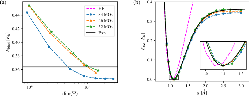
Figure 3: (a) NN CI calculated binding energy for N₂ for three different MO basis sets as a function of the dimension of the selected many-body Hilbert space. (b) dissociation curve computed with NN CI for three different sets of MOs, the Hartree-Fock reference curve, and experimental data [30]. The curves have been aligned at the minimum energy $\text{Min}\left[E_{\text{gs}}(a)\right]\equiv 0$. The inset shows a zoom around the curve minimum .

Binding energy

As a first result we present the N₂ binding energy (13), which we computed by approximating $E_{\text{gs}}(a\rightarrow\infty)\approx E_{\text{gs}}(a=3\,\text{\AA})$. In Fig. 3 (a) we plot the convergence of the NN CI result for three different sizes of the underlying MO basis. The black dashed line is the experimental value [30] of $E_{\text{bind}}=0.3638\,$E_h. Each plotted data point presents a NN selective extension step in our algorithm which increases the dimension of the Hilbert space for the ground state calculation. While we see monotonous convergence towards the experimental value upon increasing the size of the MO basis, the evolution with the NN extension steps shows quite different behaviour. For smaller basis sizes the binding energy is overestimated and converges with increased Hilbert space dimension to a slightly underestimated value. The reason for this behavior is the difference in convergence of the total energy at the equilibrium distance $a_{\text{min}}$ and at the dissociation limit $a\rightarrow\infty$.

Dissociation curve

We now turn to the result for the full dissociation curve $E_{\text{gs}}(a)$ of N₂ and compare to the experimental reference data [30] which was used to obtain a fit to a modified Morse+Lennard-Jones potential function which captures the measured frequencies of the 0-19th vibrational state (the 19th vibrational state is roughly in the middle w. r. t the depth of the well). In Fig. 3 (b) we show data up to $a=3.0\,\text{ \AA}$ including results for three different MO basis sizes as well as the Hartree-Fock curve. Overall we good agreement with the experimental curve and a monotonous convergence of the whole curve to the experimental data with increasing number of MOs (as previously also seen for $E_{\text{bind}}$). While $E_{\text{bind}}$ is known to converge quicker than the full $E_{\text{gs}}(a)$ curve due to error cancellation, our result in Fig. 3 (b) shows a good agreement of the entire curve including the dissociation limit $a\rightarrow\infty$ as well as in the region of the equilibrium distance. The inset in Fig. 3 (b) is a zoom around $a_{\text{min}}$ and shows that all NN CI calculations (within our finite $a$ grid) improve the HF value considerably towards the exact value of $a_{\text{min}}=1.098\,\text{ \AA}$ [30].

Correlation energy

Finally, as a last result, we turn to the computed correlation energy $E_{\text{corr}}$ (see (10)) at the equilibrium distance of $\approx 1.1$ Å. In Fig. 4 we show NN CI data for the three different MO bases and the convergence of $E_{\text{corr}}$ as a function of the Hilbert space dimension. In order to benchmark our results, we compare to the result of fCI calculations [2] which were obtained on a basis of approx. $10^{10}$ SDets with 34 MOs. The comparison allows for intriguing conclusions: Firstly, all presented NN CI calculations converge on basis sets of dimensionalities which are four to five orders of magnitude smaller than for the reference data. Specifically, for with 52 MOs our distance to the benchmark is less than $\approx 0.004$ E_h on only $\lesssim 2\cdot 10^{5}$ SDets. This result underlines the general feasibility of the selective scheme and the great potential for finding highly efficient many-body bases with the help of a NN classifier. Another, equally remarkable observation is that the size of the underlying MO basis can be decisive for optimal efficiency. I.e., with 52 MOs we reach the fCI benchmark significantly quicker than for 46 or 34 MOs. Indeed this observation underlines a well known dependence of CI performance on the choice of the single-particle basis and strongly motivates MO optimization, such as the correlation optimized virtual orbitals (COVO) [31], for future NN CI studies.

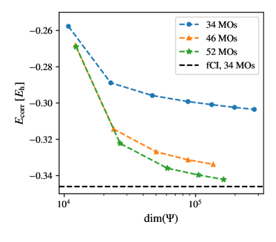
Figure 4: N₂ correlation energy computed with NN CI for three different sets of MOs. The benchmark (black dashed line) is the full CI calculation in [2] using 34 MOs which corresponds to approx. $10^{10}$ (symmetry adapted) basis SDets. All calculations were done for $2.1\,a_{0}\approx 1.111\,\mathrm{\AA}$.

IV Summary and Conclusion

In summary, we integrated Hartree-Fock calculations with the formulation of a cluster Hamiltonian to perform selective CI calculations for the paradigmatic N₂ molecule. Our method follows a very recently proposed scheme by Bilous et al. [20] and leverages active learning of a NN classifier for selectively optimizing the many-body basis. Despite the much more complex interaction tensor for the N₂ model compared to the cluster considered in [20], our calculations yielded accurate results and good agreement with experimental data as well as fCI benchmarks. Specifically we presented results for binding energies, the dissociation curve, and correlation energies. Notably, the NN CI approach successfully reproduced fCI results on significantly smaller (by four to five orders of magnitude) highly efficient bases. Besides demonstrating the potential of neural-network-supported optimization of the many-body basis, our results highlight the dramatic effect of the choice of the underlying single-particle MO basis. The number of MOs taken into account has substantial impact on the efficiency and accuracy of the CI results, suggesting that further improvements could be achieved through refined MO selection.

The computational efficiency of the neural-network-supported CI approach demonstrated here for the N₂ molecule enables highly accurate calculations across a much broader range of systems than currently possible, pushing the boundaries of CI limitations due to the exponential scaling. Future applications of the NN CI scheme include geometry optimization of atomic structures and calculations of the energy and intensity of optical transitions, where recently developed state-specific mean-field methods [32] can provide a basis of orbitals optimized for excited electronic states.

V Acknowledgements

This work was supported by the Icelandic Research Fund (grant agreements nos. 217751, 217734). Computer resources, data storage and user support were provided by the Division of Information Technology of the University of Iceland through the Icelandic Research e-Infrastructure (IREI) project, funded by the Icelandic Centre of Research infrastructure fund. The authors further gratefully acknowledge the scientific support and HPC resources provided by the Erlangen National High Performance Computing Center (NHR@FAU) of the Friedrich-Alexander-Universität Erlangen-Nürnberg (FAU).

VI Appendix

VI.1 Calculation of single- and two-particle integrals in the projector augmented wave approach

In PAW we write the so called “all-electron” states (which contain cusps at atomic centers) as

$$\varphi_{i,\sigma}(\mathbf{r})=\hat{\mathcal{T}}\tilde{\varphi}_{i,\sigma}(\mathbf{r})$$ (14)

where $\tilde{\varphi}_{i,\sigma}$ are “pseudo-electron” spin states, which are smooth everywhere. $\hat{\mathcal{T}}$ is a linear transformation operator which corrects for the smooth description of electronic states near atomic centers

$$\hat{\mathcal{T}}=1+\sum_{a}(\ket{\phi}^{a}_{\alpha}-\ket{\tilde{\phi}^{a}_{\alpha}})\bra{\tilde{p}^{a}_{\alpha}}$$ (15)

$\phi^{a}_{i}$ and $\tilde{\phi}^{a}_{i}$ are auxiliary partial waves describing the all-electron and pseudo-electron states in a region of radius $r^{a}_{c}$ around each atomic nuclei ($\hat{\mathcal{T}}$ ensures they are zero everywhere else). $p^{a}_{i}$ are smooth projection functions which satisfy

$$\braket{p^{a}_{\alpha}}{\tilde{\varphi}_{i,\sigma}}= P^{a}_{\alpha i,\sigma}$$ (16)

$$\braket{p^{a}_{\alpha}}{\tilde{\phi}^{a}_{\beta}}= \delta_{\alpha\beta}\ \ ,\ \ \text{for}\mid\mathbf{r}-\mathbf{R}^{a}\mid\leq r^{a}_{c}$$ (17)

resulting in

$$\tilde{\varphi}^{a}_{i,\sigma}= \sum_{i}P^{a}_{\alpha i,\sigma}\tilde{\phi}^{a}_{\alpha}$$ (18)

$$\varphi^{a}_{i,\sigma}= \hat{\mathcal{T}}\tilde{\varphi}^{a}_{i,\sigma}=\sum_{i}P^{a}_{\alpha i,\sigma}\phi^{a}_{\alpha}$$ (19)

i.e. the linear expansion coefficients are the same for all- and pseudo-electron states. This is general for any linear projection operator applied to PAW transformed states. It is convenient to define here an atomic density matrix, which for a given state is

$$D^{a}_{\alpha\beta i,\sigma}=P^{a*}_{\alpha i,\sigma}P^{a}_{\beta i,\sigma}$$ (20)

or similarly for any pair of states

$$D^{a}_{\alpha\beta ij,\sigma}=P^{a*}_{\alpha i,\sigma}P^{a}_{\beta j,\sigma}$$ (21)

For clarity the spin index is suppressed in the following sections.

VI.1.1 Single particle integrals in PAW

The single-particle integrals in the PAW formalism are

$$t_{ij} =\braket{\tilde{\varphi}_{i}(\mathbf{r})\mid-\frac{1}{2}\nabla^{2}\mid\tilde{\varphi}_{j}(\mathbf{r})}$$

$$+\int\tilde{n}_{ij}(\mathbf{r})\left(\tilde{V}_{\mathrm{Coul}}(\mathbf{r})+\tilde{V}_{\mathrm{XX}}(\mathbf{r})+\sum_{a}\bar{v}^{a}(\mathbf{r})\right)d\mathbf{r}$$

$$+\left(\frac{\partial\Delta E^{a}}{\partial D^{a}_{\gamma\delta ij}}+\int\tilde{V}_{\mathrm{Coul}}(\mathbf{r})\frac{\partial\tilde{\rho}(\mathbf{r})}{\partial D^{a}_{\mathrm{\gamma\delta}}}d\mathbf{r}\right)D^{a}_{\alpha\beta ij}\,,$$ (22)

where $\tilde{V}_{\mathrm{Coul}}$, $\tilde{V}_{\mathrm{XX}}$, and $\bar{v}^{a}$ are the Coulomb and exchange potentials formed by the pseudo electronic wave functions and atomic zero potentials, respectively, and $\Delta E^{a}$ are atomic corrections, as defined in Ref. 33, 26 The indexation $ij$ is carried out over the spatial electronic wave functions.

VI.1.2 Two particle integrals in PAW

The elements of the Coulomb tensor are

$$U_{ijkl}= \int d\mathbf{r}\int d\mathbf{r}^{\prime}\frac{\varphi_{i}^{*}(\mathbf{r})\varphi_{j}(\mathbf{r})\varphi^{*}_{k}(\mathbf{r}^{\prime})\varphi_{l}(\mathbf{r}^{\prime})}{\mid\mathbf{r}-\mathbf{r}^{\prime}\mid}$$ (23)

$$= \int d\mathbf{r}\int d\mathbf{r}^{\prime}\frac{n_{ij}(\mathbf{r})n_{kl}(\mathbf{r}^{\prime})}{\mid\mathbf{r}-\mathbf{r}^{\prime}\mid}\,,$$

where, for instance, $U_{iijj}$ and $U_{ijij}$ are the Coulomb and the exchange terms, respectively, and the indexation is carried out over the spatial electronic wave functions. Pair valence orbital densities are given by

$$n_{ij}(\mathbf{r}) =\braket{\varphi_{i}}{\mathbf{r}}\braket{\mathbf{r}}{\varphi_{j}}$$ (24)

$$=\tilde{n}_{ij}(\mathbf{r})+\sum_{a}(n^{a}_{ij}(\mathbf{r}^{l})-\tilde{n}^{a}_{ij}(\mathbf{r}^{l}))\,.$$ (25)

All atomic centered PAWs and densities are represented on a radial grid $\mathbf{r}^{l}$. The pseudo pair densities and atomic pseudo pair densities are modified by adding and subtracting atomic-centered compensation charges

$$n_{ij}(\mathbf{r}) =\tilde{n}_{ij}(\mathbf{r})+\sum_{a}\tilde{\mathcal{Z}}^{a}_{ij}(\mathbf{r})$$

$$+\sum_{a}((n^{a}_{ij}(\mathbf{r}^{l})-\tilde{n}^{a}_{ij}(\mathbf{r}^{l})-\tilde{\mathcal{Z}}^{a}_{ij}(\mathbf{r}^{l}))$$ (26)

to decouple corrections within different PAW regions ($aa^{\prime}$ cross terms). These compensation charges are expanded in terms of the real-space solid harmonics as

$$\tilde{\mathcal{Z}}^{a}_{ij}(\mathbf{r})=\sum_{L}\Delta^{a}_{L\alpha\beta}D^{a}_{\alpha\beta ij}\tilde{g}^{a}_{L}(\mathbf{r})\,,$$ (27)

ensuring that the atomic regions are electrostatically decoupled up to and including the quadrupole moment. The angular moment atomic expansion coefficients $\Delta^{a}_{L\alpha\beta}$ are pre-calculated and stored. This means that any corrections to the electrostatic potential are confined to the augmentation region $\left|\mathbf{r}-\mathbf{R}^{a}\right|\leq r^{a}_{c}$ and can similarly be pre-calculated and stored. Expanding Eq. (23) in terms of Eq. (26) gives

$$U_{ijkl}= \int d\mathbf{r}\int d\mathbf{r}^{\prime}\frac{(\tilde{n}_{ij}(\mathbf{r})+\tilde{\mathcal{Z}}^{a}_{ij}(\mathbf{r}))(\tilde{n}_{kl}(\mathbf{r}^{\prime})+\tilde{\mathcal{Z}}^{a}_{kl}(\mathbf{r}^{\prime}))}{\left|\mathbf{r}-\mathbf{r}^{\prime}\right|}$$

$$+\sum_{a}\int d\mathbf{r}\int d\mathbf{r}^{\prime}\frac{\Delta\rho^{a}_{ij}(\mathbf{r}^{l})\Delta\rho^{a}_{kl}(\mathbf{r}^{l^{\prime}})}{\left|\mathbf{r}^{l}-\mathbf{r}^{l^{\prime}}\right|}$$ (28)

where $\Delta\rho^{a}=n^{a}-\tilde{n}^{a}-\tilde{Z}^{a}$. The term conveniently splits up in to a pseudo and an atomic correction part

$$U_{ijkl}=\tilde{U}_{ijkl}+\sum_{a}\Delta U^{a}_{ijkl}$$ (29)

It can be shown [33] that

$$\Delta U^{a}_{ijkl}=2\sum_{\alpha\beta\gamma\delta}D^{a}_{\alpha\beta ij}C^{a}_{\alpha\beta\gamma\delta}D^{a}_{\gamma\delta kl}$$ (30)

where the atomic Coulomb kernel $C^{a}_{\alpha\beta\gamma\delta}$ is similarly pre-calculated and stored.

For the pseudo part, we define the pseudo pair-density potential

$$\tilde{\Phi}_{ij}(\mathbf{r})=\int d\mathbf{r}^{\prime}\frac{\tilde{n}_{ij}(\mathbf{r}^{\prime})+\tilde{\mathcal{Z}}^{a}_{ij}(\mathbf{r}^{\prime})}{\left|\mathbf{r}-\mathbf{r}^{\prime}\right|}\,,$$ (31)

which is solved for using standard Poisson solvers. The pseudo term is

$$\tilde{U}_{ijkl}=\int d\mathbf{r}\tilde{\Phi}_{ij}(\mathbf{r})\left(\tilde{n}_{kl}(\mathbf{r})+\tilde{\mathcal{Z}}^{a}_{kl}(\mathbf{r})\right)$$ (32)

For real-valued functions the indexes $ijkl$ are invariant according to the following symmetry operations $i\leftrightarrow j,\ \ k\leftrightarrow l,\ \ ij\leftrightarrow kl$, and any combination thereof. Note that $\tilde{n}_{ii}$ contain a net monopole ($\int\tilde{n}_{ii}dV\neq 0$). In the case of a plane-wave basis set a charge neutralizing background is added to the simulation cell (with constant value $\frac{1}{V}\int\tilde{n}_{ii}dV$) and the charge neutral electrostatic potential solved for. For all terms involving the symmetry $i=j\wedge k=l$ the shift in energy due to the charge neutralization is corrected afterwards.

VI.2 NN-supported CI: Architecture and implementation

For the basis state selection procedure we employ a NN classifier of the convolutional type [28], see Fig. 1. The NN receives candidate SDets $\ket{\phi_{\alpha}}$ in occupation number representation, i.e. strings of 0s and 1s, as an input (A). The input is split into two spin channels and then passes through a filter kernel of size 2 (B), generating 64 feature maps (C). These maps are subsequently processed by a kernel of size 1, resulting in 4 output channels (D). The output is flattened and forwarded to a dense block (E) which ends with an output layer consisting of two neurons (F). These neurons classify the input SDet as “important” or “unimportant” by applying a softmax activation function. The latter ensures that the outputs lie between 0 and 1 and sum up to 1, and are therefore interpretable as the corresponding probabilities.

In all hidden NN layers the rectified linear unit (ReLU) is employed as the activation function, and the network’s performance is evaluated using categorical cross-entropy. The Adam algorithm [34] is used for training, which terminates after no improvement is observed over three consecutive epochs, a method known as “early stopping with patience”. This architecture has been previously demonstrated to be efficient for solving the configuration interaction (CI) problem [19, 20]. For further comprehensive details of the iterative algorithm and computational protocol, we refer to [20].

The NN implementation was carried out using the Python libraries JAX [35] and FLAX [36]. We integrated this NN block in a common pipeline with our CI solver. The latter was implemented using the JAX [35], NumPy [37], Pandas [38] and SciPy [39] libraries.

References

- Szabo and Ostlund [2012] A. Szabo and N. Ostlund, Modern Quantum Chemistry: Introduction to Advanced Electronic Structure Theory, Dover Books on Chemistry (Dover Publications, 2012).
- Rossi et al. [1999] E. Rossi, G. L. Bendazzoli, S. Evangelisti, and D. Maynau, A full-configuration benchmark for the n2 molecule, Chemical Physics Letters 310, 530 (1999).
- Kohn and Sham [1965] W. Kohn and L. J. Sham, Self-consistent equations including exchange and correlation effects, Phys. Rev. 140, 1133 (1965).
- Hohenberg and Kohn [1964] P. Hohenberg and W. Kohn, Inhomogeneous electron gas, Phys. Rev. 136, B864 (1964).
- Libisch et al. [2014] F. Libisch, C. Huang, and E. Carter, Embedded correlated wavefunction schemes: theory and applications, Acc. Chem. Res. 47, 2768 (2014).
- Jones et al. [2020] L. O. Jones, M. A. Mosquera, G. C. Schatz, and M. A. Ratner, Embedding methods for quantum chemistry: Applications from materials to life sciences, J. Am. Chem. Soc. 142, 3281 (2020).
- Ivanic and Ruedenberg [2001] J. Ivanic and K. Ruedenberg, Identification of deadwood in configuration spaces through general direct configuration interaction, Theor. Chem. Acc. 106, 339 (2001).
- Huron et al. [1973] B. Huron, J. P. Malrieu, and P. Rancurel, Iterative perturbation calculations of ground and excited state energies from multiconfigurational zeroth‐order wavefunctions, The Journal of Chemical Physics 58, 5745 (1973), https://pubs.aip.org/aip/jcp/article-pdf/58/12/5745/18885418/5745_1_online.pdf .
- Greer [1998] J. Greer, Monte carlo configuration interaction, Journal of Computational Physics 146, 181 (1998).
- Garniron et al. [2018] Y. Garniron, A. Scemama, E. Giner, M. Caffarel, and P.-F. Loos, Selected configuration interaction dressed by perturbation, The Journal of Chemical Physics 149, 064103 (2018), https://pubs.aip.org/aip/jcp/article-pdf/doi/10.1063/1.5044503/13501037/064103_1_online.pdf .
- Tubman et al. [2020] N. M. Tubman, C. D. Freeman, D. S. Levine, D. Hait, M. Head-Gordon, and K. B. Whaley, Modern approaches to exact diagonalization and selected configuration interaction with the adaptive sampling ci method, Journal of Chemical Theory and Computation 16, 2139 (2020), pMID: 32159951, https://doi.org/10.1021/acs.jctc.8b00536 .
- Coe [2018] J. P. Coe, Machine learning configuration interaction, J. Chem. Theory Comput. 14, 5739 (2018), pMID: 30285426, https://doi.org/10.1021/acs.jctc.8b00849 .
- Jeong et al. [2021] W. Jeong, C. A. Gaggioli, and L. Gagliardi, Active learning configuration interaction for excited-state calculations of polycyclic aromatic hydrocarbons, Journal of Chemical Theory and Computation 17, 7518 (2021).
- Pineda Flores [2021] S. D. Pineda Flores, Chembot: A machine learning approach to selective configuration interaction, Journal of Chemical Theory and Computation 17, 4028 (2021), pMID: 34125549, https://doi.org/10.1021/acs.jctc.1c00196 .
- Goings et al. [2021] J. J. Goings, H. Hu, C. Yang, and X. Li, Reinforcement learning configuration interaction, Journal of Chemical Theory and Computation 17, 5482 (2021), pMID: 34423637, https://doi.org/10.1021/acs.jctc.1c00010 .
- Herzog et al. [2023] B. Herzog, B. Casier, S. Lebegue, and D. Rocca, Solving the schrödinger equation in the configuration space with generative machine learning, Journal of Chemical Theory and Computation 19, 2484 (2023), https://doi.org/10.1021/acs.jctc.2c01216 .
- Coe [2019] J. P. Coe, Machine learning configuration interaction for ab initio potential energy curves, J. Chem. Theory Comput. 15, 6179 (2019).
- Molchanov et al. [2022] O. M. Molchanov, K. D. Launey, A. Mercenne, G. H. Sargsyan, T. Dytrych, and J. P. Draayer, Machine learning approach to pattern recognition in nuclear dynamics from the ab initio symmetry-adapted no-core shell model, Phys. Rev. C 105, 034306 (2022).
- Bilous et al. [2023] P. Bilous, A. Pálffy, and F. Marquardt, Deep-learning approach for the atomic configuration interaction problem on large basis sets, Phys. Rev. Lett. 131, 133002 (2023).
- Bilous et al. [2024] P. Bilous, L. Thirion, H. Menke, M. W. Haverkort, A. Pálffy, and P. Hansmann, Neural-network-supported basis optimizer for the configuration interaction problem in quantum many-body clusters: Feasibility study and numerical proof (2024), arXiv:2406.00151 [cond-mat.str-el] .
- Blöchl [1994] P. E. Blöchl, Projector augmented-wave method, Physical Review B 50, 17953 (1994).
- Blöchl et al. [2003] P. E. Blöchl, C. J. Först, and J. Schimpl, Projector augmented wave method:ab initio molecular dynamics with full wave functions, Bulletin of Materials Science 26, 33 (2003).
- Larsen et al. [2009] A. H. Larsen, M. Vanin, J. J. Mortensen, K. S. Thygesen, and K. W. Jacobsen, Localized atomic basis set in the projector augmented wave method, Phys. Rev. B, Condens. Matter 80, 195112 (2009).
- Ivanov et al. [2021a] A. V. Ivanov, E. Ö. Jónsson, T. Vegge, and H. Jónsson, Direct energy minimization based on exponential transformation in density functional calculations of finite and extended systems, Computer Physics Communications 267, 108047 (2021a).
- Ivanov et al. [2021b] A. V. Ivanov, G. Levi, E. Ö. Jónsson, and H. Jónsson, Method for calculating excited electronic states using density functionals and direct orbital optimization with real space grid or plane-wave basis set, Journal of Chemical Theory and Computation 17, 5034 (2021b).
- Mortensen et al. [2024] J. J. Mortensen, A. H. Larsen, M. Kuisma, A. V. Ivanov, A. Taghizadeh, A. Peterson, A. Haldar, A. O. Dohn, C. Schäfer, E. Ö. Jónsson, E. D. Hermes, F. A. Nilsson, G. Kastlunger, G. Levi, H. Jónsson, H. Häkkinen, J. Fojt, J. Kangsabanik, J. Sødequist, J. Lehtomäki, J. Heske, J. Enkovaara, K. T. Winther, M. Dulak, M. M. Melander, M. Ovesen, M. Louhivuori, M. Walter, M. Gjerding, O. Lopez-Acevedo, P. Erhart, R. Warmbier, R. Würdemann, S. Kaappa, S. Latini, T. M. Boland, T. Bligaard, T. Skovhus, T. Susi, T. Maxson, T. Rossi, X. Chen, Y. L. A. Schmerwitz, J. Schiøtz, T. Olsen, K. W. Jacobsen, and K. S. Thygesen, Gpaw: An open python package for electronic structure calculations, The Journal of Chemical Physics 160, 092503 (2024).
- Murphy [2022] K. P. Murphy, Probabilistic Machine Learning: An introduction (MIT Press, 2022).
- Goodfellow et al. [2016] I. Goodfellow, Y. Bengio, and A. Courville, Deep Learning (MIT Press, 2016) http://www.deeplearningbook.org.
- Kolos and Wolniewicz [1965] W. Kolos and L. Wolniewicz, Potential-energy curves for the x, b, and c states of the hydrogen molecule, The Journal of Chemical Physics 43, 2429 (1965).
- Le Roy et al. [2006] R. J. Le Roy, Y. Huang, and C. Jary, An accurate analytic potential function for ground-state n2 from a direct-potential-fit analysis of spectroscopic data, The Journal of Chemical Physics 125, 164310 (2006).
- Bylaska et al. [2021] E. J. Bylaska, D. Song, N. P. Bauman, K. Kowalski, D. Claudino, and T. S. Humble, Quantum solvers for plane-wave hamiltonians: Abridging virtual spaces through the optimization of pairwise correlations, Frontiers in Chemistry 9, 10.3389/fchem.2021.603019 (2021).
- Levi et al. [2020] G. Levi, A. V. Ivanov, and H. Jónsson, Variational density functional calculations of excited states via direct optimization, J. Chem. Theory Comput. 16, 6968 (2020).
- Mortensen et al. [2005] J. J. Mortensen, L. B. Hansen, and K. W. Jacobsen, Real-space grid implementation of the projector augmented wave method, Phys. Rev. B 71, 035109 (2005).
- Kingma and Ba [2017] D. P. Kingma and J. Ba, Adam: A method for stochastic optimization (2017), arXiv:1412.6980 [cs.LG] .
- Bradbury et al. [2018] J. Bradbury, R. Frostig, P. Hawkins, M. J. Johnson, C. Leary, D. Maclaurin, G. Necula, A. Paszke, J. VanderPlas, S. Wanderman-Milne, and Q. Zhang, JAX: composable transformations of Python+NumPy programs (2018).
- Heek et al. [2023] J. Heek, A. Levskaya, A. Oliver, M. Ritter, B. Rondepierre, A. Steiner, and M. van Zee, Flax: A neural network library and ecosystem for JAX (2023).
- Harris et al. [2020] C. R. Harris, K. J. Millman, S. J. van der Walt, R. Gommers, P. Virtanen, D. Cournapeau, E. Wieser, J. Taylor, S. Berg, N. J. Smith, R. Kern, M. Picus, S. Hoyer, M. H. van Kerkwijk, M. Brett, A. Haldane, J. F. del Río, M. Wiebe, P. Peterson, P. Gérard-Marchant, K. Sheppard, T. Reddy, W. Weckesser, H. Abbasi, C. Gohlke, and T. E. Oliphant, Array programming with NumPy, Nature 585, 357 (2020).
- Wes McKinney [2010] Wes McKinney, Data Structures for Statistical Computing in Python, in Proceedings of the 9th Python in Science Conference, edited by Stéfan van der Walt and Jarrod Millman (2010) pp. 56 – 61.
- Virtanen et al. [2020] P. Virtanen, R. Gommers, T. E. Oliphant, M. Haberland, T. Reddy, D. Cournapeau, E. Burovski, P. Peterson, W. Weckesser, J. Bright, S. J. van der Walt, M. Brett, J. Wilson, K. J. Millman, N. Mayorov, A. R. J. Nelson, E. Jones, R. Kern, E. Larson, C. J. Carey, İ. Polat, Y. Feng, E. W. Moore, J. VanderPlas, D. Laxalde, J. Perktold, R. Cimrman, I. Henriksen, E. A. Quintero, C. R. Harris, A. M. Archibald, A. H. Ribeiro, F. Pedregosa, P. van Mulbregt, and SciPy 1.0 Contributors, SciPy 1.0: Fundamental Algorithms for Scientific Computing in Python, Nature Methods 17, 261 (2020).