Probing Implicit Bias in Semi-gradient Q-learning: Visualizing the Effective Loss Landscapes via the Fokker–Planck Equation

Abstract

Semi-gradient Q-learning is applied in many fields, but due to the absence of an explicit loss function, studying its dynamics and implicit bias in the parameter space is challenging. This paper introduces the Fokker–Planck equation and employs partial data obtained through sampling to construct and visualize the effective loss landscape within a two-dimensional parameter space. This visualization reveals how the global minima in the loss landscape can transform into saddle points in the effective loss landscape, as well as the implicit bias of the semi-gradient method. Additionally, we demonstrate that saddle points, originating from the global minima in loss landscape, still exist in the effective loss landscape under high-dimensional parameter spaces and neural network settings. This paper develop a novel approach for probing implicit bias in semi-gradient Q-learning.

1 Introduction

Q-learning, a classic Reinforcement Learning (RL) algorithm, is often paired with function approximation, such as the Deep Q-Network (DQN) [1]. This algorithm finds applications in various domains, including gaming [1, 2, 3], recommendation systems [4], and combinatorial optimization [5, 6]. The primary objective of Q-learning is to minimize an empirical Bellman optimal loss. The semi-gradient method is commonly employed to minimize this loss. The semi-gradient approach deviates from the exact gradient by omitting the term involving the maximum operation, converge fast but potentially leading to divergence [7, 8, 9, 10]. In contrast, the residual gradient method  [11] represents the precise gradient of the loss, it offers stability but converge slowly. Moreover, when training the model with partial data, such as through mini-batch and replay buffer techniques [1], these two methods may converge to different policies [12, 13]. Additionally, the semi-gradient method is more prevalent in practical applications. Motivated by this success, we want to investigate the implicit bias of semi-gradient Q-learning.

The research on implicit bias [14] contains following directions: the relationship between over-parameterization and generalization [15], properties of the parameters of learned neural networks [16], and different preferences of algorithm for critical points [17]. These studies primarily concentrate on supervised learning and rely on the gradient flow of a explicit loss function. However, due to the absence of a corresponding explicit loss function for the semi-gradient, employing the analytical methodologies common in supervised learning is unfeasible. To address the challenge, we employ the Fokker–Planck Equation (FPE) [18, 19] to establish the effective loss landscape and subsequently visualize it. In fields like biology and statistical mechanics, the FPE is utilized to depict the effective loss landscape in scenarios involving non-conservative forces, where the force does not align with the negative gradient of any specific loss function (further details in Appendix A). Given that the semi-gradient can be viewed as a non-conservative force, we leverage the FPE to construct an effective loss landscape for it. Our approach involves initially constructing the effective loss landscape and then showcasing the implicit bias of the semi-gradient method through training dynamics.

Figure 1 illustrates the (effective) loss landscape and training dynamics associated with both the residual gradient and semi-gradient method. Due to the utilization of only partial data for constructing the loss landscape, two solutions emerge within it, represented by orange and blue stars. Notably, the training dynamics of the residual gradient method in (a) exhibit a stark contrast to those of the semi-gradient method in (b). Furthermore, the training dynamics for the semi-gradient method diverge, showcasing an exponential increase in loss, as depicted in (c). Upon comparing (a) and (b), it becomes apparent that the blue star transitions from a global minimum to a saddle point. This straightforward example offers valuable insights into the distinct implicit biases exhibited by the semi-gradient method compared to the residual gradient method when trained with partial data.

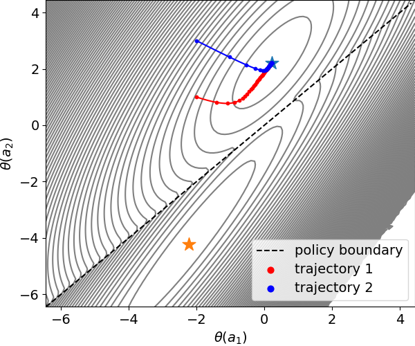
(a) training dynamics of residual gradient method

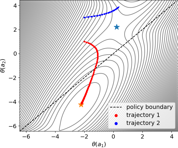
(b) training dynamics of semi-gradient method

Figure 1: The training dynamics of two methods initiate from the points $(-2,1)$ (red) and $(-2,3)$ (blue) within the landscape constructed using the data $\{(s_{1},a_{1},s_{2},r),(s_{1},a_{2},s_{3},r)\}$ from Example 3.1. In (a), both trajectories converge to $\theta_{\pi_{1}}$. Conversely, in (b), all the trajectories bias against $\theta_{\pi_{2}}$.

Main Contributions: 1) Visualization and Analysis of the Effective Loss Landscape and Implicit Bias in $\mathbb{R}^{2}$ Parameter Space: We introduced Wang’s potential landscape theory [18] to explore the effective loss landscape of the semi-gradient method. This approach enabled us to visualize the effective loss landscape and help us to analyze the implicit bias. We highlight two key insights: first, the semi-gradient method may transform certain global minima into a saddle point when only partial data is available; second, the gradient of the state-action value function $Q$ can influence the position of the saddle points. 2) Extension of Implicit Bias Understanding to Higher Dimensions: We have shown that the implicit bias observed with the semi-gradient method is also present in high-dimensional parameter spaces and neural networks. This extends our comprehension of implicit bias into more complex and higher-dimensional spaces. 3) Development of a Novel Approach for Probing Implicit Bias in Semi-gradient Q-learning: Our approach comprises three steps: initially, we introduce a visualization tool to detect implicit bias in a simple example; next, we establish an intuitive grasp of the implicit bias; and finally, we design experimental procedures for high-dimensional scenarios to demonstrate the presence of implicit bias. All the code related to this research is available on GitHub at https://github.com/dayhost/FPE.

2 Related Works

Our research is closely related with the comparative analysis of the residual and semi-gradient methods. Schoknecht et al. [20] and Li et al. [21] have examined the convergence rates of the residual and semi-gradient methods in policy evaluation within a linear approximation framework. Saleh et al. [12] have compared the policies learned by residual and semi-gradient Q-learning in both deterministic and stochastic environments. Furthermore, Zhang et al. [13] integrated the residual gradient method into DDPG [22] and achieved improved performance in the DeepMind Control Suite compared to DDPG utilizing the semi-gradient method.

The investigation of implicit bias is relevant to this study. An initial exploration of implicit bias was conducted by Neyshabur el al [23], it demonstrates that the capacity-controlling property of neural networks can lead to improved generalization. Similarly, Belkin el al [15] discovered the phenomenon of double descent, indicating that neural networks in over-parameterized regime exhibit better generalization as the number of parameters increases. Ergen el al [16] analyzes the properties of critical points of two-layer neural networks with regularized loss. Keskar et al [17] found that the stochastic gradient descent (SGD) method often converges to flatter local minima, enhancing the generalization ability of neural networks. Current research on implicit bias predominantly focuses on supervised learning, while this work aims to discuss implicit bias in the realm of reinforcement learning.

The methodology for modeling non-equilibrium loss landscapes is also relevant to our research. Wang et al. [18] introduced Wang’s potential landscape theory for constructing effective loss landscapes, a method we employ in our work. Additionally, Zhou et al. [19] outlined three approaches for constructing effective loss landscapes, including Wang’s potential landscape theory, the Freidlin-Wentzell quasi-potential method, and the A-type integral method.

3 Effective Loss Landscape Visualization and Implicit Bias Demonstration

Before dive into the loss landscape, we initially define the empirical Bellman optimal loss, residual gradient, and semi-gradient. The empirical Bellman optimal loss is defined as $\mathcal{L}=\frac{1}{|\mathcal{D}|}\sum_{(s,a,s^{\prime},r)\in\mathcal{D}}\left(Q(s,a)-r(s,a)-\gamma\max_{a^{\prime}\in A}Q(s^{\prime},a^{\prime})\right)^{2}$, where $s\in S$ represents a state, $S$ denotes the state space, $a\in A$ signifies an action, $A$ denotes the action space, $r:S\times A\to\mathbb{R}$ symbolizes the reward function, $\mathcal{D}$ denotes the sample dataset, $Q:S\times A\to\mathbb{R}$ stands for the state value function, and $\gamma\in(0,1)$ represents the discount factor. The semi-gradient is defined as $\nabla\mathcal{L}_{\rm{semi}}=\frac{2}{|\mathcal{D}|}\sum_{(s,a,s^{\prime},r)\in\mathcal{D}}\nabla Q(s,a)\left(Q(s,a)-r(s,a)-\gamma\max_{a^{\prime}\in A}Q(s^{\prime},a^{\prime})\right).$ The residual gradient is defined as $\nabla\mathcal{L}_{\rm{res}}=\frac{2}{|\mathcal{D}|}\sum_{(s,a,s^{\prime},r)\in\mathcal{D}}\left(\nabla Q(s,a)-\nabla\max_{a^{\prime}\in A}Q(s^{\prime},a^{\prime})\right)$ $\left(Q(s,a)-r(s,a)-\gamma\max_{a^{\prime}\in A}Q(s^{\prime},a^{\prime})\right).$

3.1 Setting and one solution scenario

In this subsection, we present an example to illustrate the visualization of loss landscapes. All figures depicting loss landscapes in this section are based on the settings outlined in Example 3.1.

Example 3.1 (example for visualization).

Consider a deterministic Markov Decision Process (MDP) $\mathcal{M}(S,A,f,r,\gamma)$ with three states $S=\{s_{1},s_{2},s_{3},s_{4}\}$ and two actions $A=\{a_{1},a_{2}\}$. State $s_{4}$ serves as a terminal state, and the transition function $f:\{s_{1},s_{2},s_{3}\}\times\{a_{1},a_{2}\}\to\{s_{1},s_{2},s_{3},s_{4}\}$ is illustrated in Figure 2. The reward function $r:\{s_{1},s_{2},s_{3}\}\times\{a_{1},a_{2}\}\to\mathbb{R}$ is defined along each transition path. The discount factor is denoted as $\gamma\in(0,1)$. Specifically, we fix $\gamma=0.9$ and set $r(s,a)=-0.1$ for all $(s,a)\in\{s_{1},s_{2},s_{3}\}\times\{a_{1},a_{2}\}$. For simplicity, we define $r:=r(s,a)$.

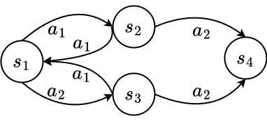
Figure 2: The geometric structure of the given MDP environment.

Parameterization of $Q$. Our primary approach involves employing a linear model with two parameters to approximate the $Q$ function. These parameters are denoted as $\theta=[\theta(a_{1}),\theta(a_{2})]^{\text{T}}$, where $\theta(a_{1}),\theta(a_{2})\in\mathbb{R}$, to parameterize $Q$. This function can be expressed as the product of the state embedding and parameters: $Q(s,a)=\phi(s)\theta(a)$, where $\phi(s)\in\mathbb{R}$ represents the state embedding of state $s$. Specifically, we assume $\phi(s_{1})=0.1$, $\phi(s_{2})=11/180$ and $\phi(s_{3})=29/180$. Given that all state embeddings are positive, only two policies can be defined: $\pi_{1}(s_{1})=a_{1},\pi_{1}(s_{2})=a_{1}$ and $\pi_{2}(s_{1})=a_{2},\pi_{2}(s_{2})=a_{2}$. The equality $\theta(a_{1})=\theta(a_{2})$ delineates the policy boundary.

Remark 3.2.

In many theoretical analyses of Q-learning with linear approximation, the state-value function is typically denoted as $Q(s,a)=\phi(s,a)\theta$, where $\phi(s,a)\in\mathbb{R}^{d}$ and $\theta\in\mathbb{R}^{d}$. However, in the practical implementation of DQN, the input data consists of state embeddings that depend solely on the state, while the output is a vector representing the action values for the given state. We adopt the setting in DQN. Additionally, we assume that $\phi(s_{1}),\phi(s_{2}),\phi(s_{3})>0$. This assumption stems from the interpretation that the output of the second-to-last layer in a neural network utilizing ReLU activation can be considered as the state embedding, where the elements are non-negative.

Settings for numerical calculation. The "force" in the Fokker–Planck equation is the negative residual or semi-gradient associated with different policies, i.e., (1), (2), (3), and (4). To facilitate the solution of the equation using the numerical method [24], this "force" is discretized into a force matrix with dimensions of $100\times 100$. Additionally, the probability distribution is discretized into a matrix with same size. The resolution of this discretization is $0.095$, and the propagation time required to determine the stationary distribution is $100,000$. The loss landscape, computed via the Fokker–Planck equation, is also influenced by a diffusion constant $\sigma$. As $\sigma\to 0$, the effective loss landscape converges towards the true static effective loss landscape. However, a smaller diffusion constant necessitates significantly greater computational resources. Hence, we opt for a sufficiently small diffusion constant, specifically $\sigma=2^{-8}$. The discretization process and the presence of a non-zero diffusion constant introduce a manageable level of numerical error to the visualization. Besides, we use an NVIDIA GeForce RTX 3080 GPU to do numerical calculation.

Data sampling strategy. In practical applications, training data is sampled from the environment, often containing only a subset of environmental’s data. Moreover, different sample data can influence the loss landscape and training dynamics. To demonstrate the (effective) loss landscape of different data, we designed the following sampling strategy: we sample one data point each containing $a_{1}$ and $a_{2}$, forming a mini-batch denoted as $\{(s_{\alpha},a_{1},s^{\prime}_{\alpha},r),(s_{\beta},a_{2},s^{\prime}_{\beta},r)\}$, and visualize it. The current sampling strategy yields a total of nine possible mini-batches, with five mini-batches having one solution and four mini-batches having two solutions. The figures of the loss landscape that were not presented in the main content are displayed in Appendix C. We define the solution within the region $\{\theta\in\mathbb{R}^{2}|\theta(a_{1})\geq\theta(a_{2})\}$ as $\theta_{\pi_{1}}$ and the solution within the region $\{\theta\in\mathbb{R}^{2}|\theta(a_{1})\leq\theta(a_{2})\}$ as $\theta_{\pi_{2}}$. The conditions for the existence of these two solutions are outlined in Lemma 5.2.

One solution scenario and smoothness of effective loss landscape. When there is only one critical point, it will be a global minimum in loss landscape, while in the effective loss landscape, this critical point could potentially be a global minimum (as shown in Figure 3), or a saddle point (as shown in Figure 11). However, since the scenario of having only one critical point is rare in high-dimensional cases, we only provide one example to illustrate the smoothness of the effective loss landscape. Figure 3 is generated using the mini-batch $\{(s_{1},a_{1},s_{2},r),(s_{2},a_{2},s_{4},r)\}$. $\theta(a_{1})$ is the abscissa, and $\theta(a_{2})$ is the ordinate. In the Figure 3, the term "force" denotes the negative residual or the semi-gradient. The "gradient" refers to the negative gradient of both the loss and the effective loss landscapes. Within the context of the loss landscape, "force" is equivalent to "gradient". The "flux" is defined as the discrepancy between "force" and "gradient". Nonetheless, the "flux" within the loss landscape is non-zero, attributable to numerical error. Detailed definitions are given in Appendix A. A comparison between (a) and (b) reveals that the contour in (a) exhibits a "heart shape," indicating the influence of the policy boundary on the loss landscape. In contrast, the contour in (b) is unaffected by the policy boundary. The shape of the contour suggests a non-smooth loss landscape, while the effective loss landscape is smooth, a notion supported by Lemma 5.4.

(a) loss landscape

(b) effective loss landscape

Figure 3: Loss landscape with the mini-batch $\{(s_{1},a_{1},s_{2},r)$, $(s_{2},a_{2},s_{4},r)\}$ and only $\theta_{\pi_{2}}$ exists. In (a), the region surrounding the global minimum exhibits a "heart" shape and lacks smoothness. Conversely, the effective loss landscape in (b) is smooth. Despite the difference of smoothness between (a) and (b), their landscape shapes are similar.

3.2 Effective loss landscapes with two solutions

In this section, we further the discussion utilizing the parameters defined in Example 5.1 and illustrate the notable distinction between the loss landscapes associated with two solutions.

Transition of global minima to saddle point. For the mini-batch $\{(s_{1},a_{1},s_{2},r)$, $(s_{1},a_{2},s_{3},r)\}$, since $\phi(s_{1})-\gamma\phi(s_{2})>0$ and $\phi(s_{1})-\gamma\phi(s_{3})<0$, according to Lemma 5.2, the Bellman optimal loss has two solutions. Figure 4 is constructed with the mini-batch. In Figure 4 (a), the two solutions $\theta_{\pi_{1}}$ and $\theta_{\pi_{2}}$ (orange and blue stars) are two global minima, and the policy boundary separates these two global minima. However, in Figure 4 (b), the contours reveal that while $\theta_{\pi_{1}}$ remains a global minimum, $\theta_{\pi_{2}}$ transitions into a saddle point. The position of the saddle point is consistent with statement $(1)$ of Theorem 5.6.

(a) loss landscape

(b) effective loss landscape

Figure 4: Loss landscapes with the mini-batch $\{(s_{1},a_{1},s_{2},r)$, $(s_{1},a_{2},s_{3},r)\}$, both $\theta_{\pi_{1}}$ (orange star) and $\theta_{\pi_{2}}$ (blue star) exist. In (a), two exact solutions are considered as two global minima. However in (b), $\theta_{\pi_{1}}$ is considered as a global minima but $\theta_{\pi_{2}}$ is considered as a saddle point.

Displacement of the saddle point. For the mini-batch $\{(s_{2},a_{1},s_{1},r)$, $(s_{2},a_{2},s_{4},r)\}$, given that $\phi(s_{2})-\gamma\phi(s_{1})<0$ and $\phi(s_{2})-\gamma\phi(s_{4})>0$, by Lemma 5.2 there are two solutions. Figure 5 is constructed with the mini-batch. In Figure 5 (a), two global minima still exist, but in Figure 5 (b), the contours reveal that $\theta_{\pi_{1}}$ (represented by the orange star) became a saddle point. A comparison between Figure 4 (b) and Figure 5 (b) shows that the saddle point has displaced from $\theta_{\pi_{2}}$ to $\theta_{\pi_{1}}$. The position of the saddle point is consistent with statement $(2)$ of Theorem 5.6.

(a) loss landscape

(b) effective loss landscape

Figure 5: Loss landscapes with the mini-batch $\{(s_{2},a_{1},s_{1},r)$, $(s_{2},a_{2},s_{4},r)\}$, both $\theta_{\pi_{1}}$ (orange star) and $\theta_{\pi_{2}}$ (blue star) exist. Compare with Figure 4, the saddle point shifted from $\theta_{\pi_{2}}$ to $\theta_{\pi_{1}}$.

Intuitive understanding of the existence of saddle point. Here, our focus lies on the presence of saddle points when multiple solutions exist in the effective loss landscape, a common occurrence in high-dimensional parameter spaces. Let’s first consider the two-dimensional scenario. Intuitively speaking, due to the presence of solutions on both sides of the policy boundary and the absence of other critical points on the effective loss landscape, the smoothness of the effective loss landscape results in a "connectivity" between the two solutions, allowing for a path from one solution to the other. This connectivity gives rise to the emergence of saddle points.. We can further speculate on the existence of saddle points in higher dimensions based on the above understanding. When solutions exist on both sides of a certain policy boundary and there are no other critical points nearby, saddle points will emerge. As shown in Figure 7 (a) and Figure 9 (a), the trajectory need to go cross the policy boundary to converge to another critical point.

3.3 Divergence and implicit bias of the semi-gradient method

After demonstrating the effective loss landscape and comparing its differences with the loss landscape, we are prepared to unveil the implicit bias of the semi-gradient method in both two-dimensional and high-dimensional scenario.

Semi-gradient method bias against a saddle point. Here, we start from the two-dimensional scenario. Figure 6 is generated with mini-batch $\{(s_{1},a_{1},s_{2},r),(s_{1},a_{2},s_{3},r)\}$. With a fixed learning rate of $0.1$ and a start point $(-2,1)$, we initially train the model using the residual gradient descent(red) for 25,000 steps ($t_{1}$). Afterwards, we switch to the semi-gradient descent(blue) and continue training for another 25,000 steps. Figure 6 (a) displays the loss landscape and the training dynamics. It is noticeable that after transit to the semi-gradient method, the training dynamics escape from $\theta_{\pi_{2}}$, cross the policy boundary at time $t_{2}$, and converge to $\theta_{\pi_{1}}$. This behavior also implies that $\theta_{\pi_{2}}$ is a saddle point for effective landscape. In Figure 6 (b), a significant alteration in the state value is observed after the switch to the semi-gradient method. Combining Figure 6 (a) and (c), it is evident that the loss reaches its apex when the training dynamics cross the policy boundary. The training trajectory of the semi-gradient descent in Figure 6 (a) consist with the statement given in Theorem 5.6.

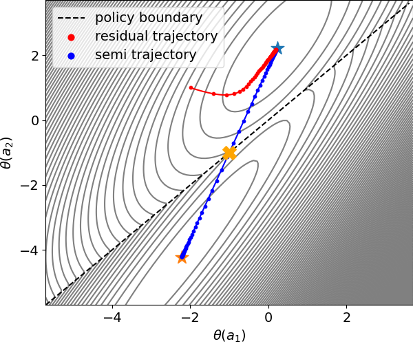
(a) trajectories

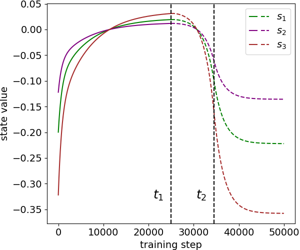
(b) state value

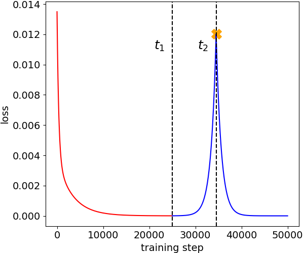
(c) loss

Figure 6: Training dynamics of two methods with the mini-batch $\{(s_{1},a_{1},s_{2},r),(s_{1},a_{2},s_{3},r)\}$. Initially, we employ residual gradient descent (red) for $25,000$ ($t_{1}$) steps, followed by a transition to semi-gradient descent (blue) for another $25,000$ steps. In (a), the dynamics converge towards $\theta_{\pi_{2}}$ under residual gradient descent, but exhibit a bias against $\theta_{\pi_{2}}$ towards $\theta_{\pi_{1}}$ under semi-gradient descent. In (b), the state values undergo significant changes after the transition. A comparison between (a) and (b) reveals that under semi-gradient descent, when the dynamics cross the policy boundary ($t_{2}$), the loss is the maxima.

Semi-gradient method bias against a saddle point in high dimension. We expand the experiment to a high-dimensional parameter space. Figure 7 is also generated by the data set $\{(s_{1},a_{1},s_{2},r)$, $(s_{1},a_{2},s_{3},r)\}$, but under a DQN setting. The $Q$ is approximated by a two-layer fully connected neural network with $100$ neurons. During initialization, each neuron in the first layer was set with a weight of $1.6$ and a bias of $-0.001$, while each neuron in the second layer was set with a weight of $0.01$ and a bias of $-0.001$. Given these initial conditions and a constant learning rate of $0.002$, we first using residual gradient descent for $10,000$ steps ($t_{1}$), followed by semi-gradient descent for another $10,000$ steps. Figure 7 (a) shows the action with maximum value for three states during the training process. In comparison with Figure 7 (c), the loss reach the maxima when cross the policy boundary($t_{2}$), which is similar with Figure 6. In addition, the dynamics of state values in Figure 7 (b) is also similar with Figure 6 (b). These similarities suggest that the convergence position of the residual gradient descent is a saddle point on the effective loss landscape.

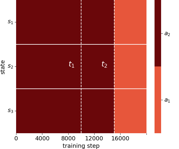
(a) policy

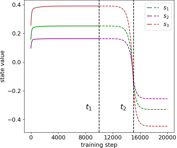
(b) state value

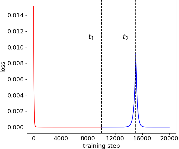
(c) loss

Figure 7: The training dynamics of two methods with the mini-batch $\{(s_{1},a_{1},s_{2},r),(s_{1},a_{2},s_{3},r)\}$ involve a neural network. Initially, we employ residual gradient descent for $10,000$ ($t_{1}$) steps and then transition to semi-gradient descent for another $10,000$ steps. In (a), the action with maximum state value for each state during training is demonstrated. A comparison between (a) and (c) reveals that the dynamics cross the policy boundary when the loss reaches its peak ($t_{2}$). This implies that the saddle point and the global minima that semi-gradient converges are situated on opposite sides of the policy boundary. (b) illustrates a significant change in state values after switching to semi-gradient descent. The observations above indicate that the residual gradient descent converges to a saddle point, and this saddle point, along with the global minima to which the semi-gradient converges, is located on opposite sides of the policy boundary.

4 Implicit Bias of the Semi-gradient Method with More Realistic Data

Example 4.1 (a grid world environment).

Given a grid world environment as illustrated in Figure 8, the state space $S$ consists of $19$ states, with $s_{16}$ being the terminal state. The action space $A=\{a_{1},a_{2},a_{3},a_{4}\}$ corresponds to the directions "up, down, left, right," respectively. When a state is at the boundary, an action that would cross this boundary results in a bounce-back to the current state, i.e., $f(s_{1},a_{1})=s_{1}$. The reward function is defined as follows: a reward of $-1$ is given when the next state is $s_{12}$, $s_{13}$, or $s_{14}$, and a reward of $+1$ is granted when the next state is $s_{15}$. The discount factor is set to $\gamma=0.98$.

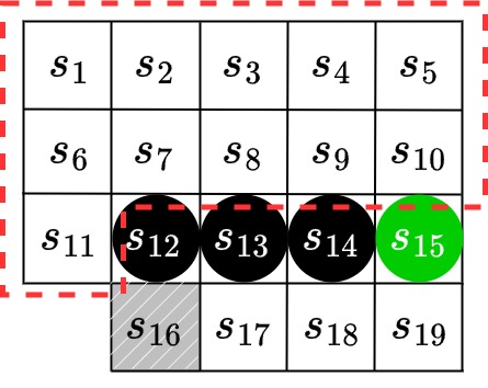
Figure 8: A grid world environment.

Data sampling strategy and neural network settings. In order to demonstrate the existence of saddle point in a larger sample dataset, we consider a mini-batch contains the Cartesian product of all states within the red box in Figure 8 and the entire action space, which has totally 44 sample data. The embeddings for these 15 states are represented by a randomly sampled $15\times 15$ matrix, and after sampling, each row is normalized. The random seed used for sampling is $4$. Furthermore, we employ a four-layer fully connected network to approximate the $Q$ function, where the first hidden layer has a width of 512, the second hidden layer has a width of 1024, and the third hidden layer has a width of 1024. The model is initialized with random seed $75$. Additionally, we use an NVIDIA GeForce RTX 3080 GPU to train the model.

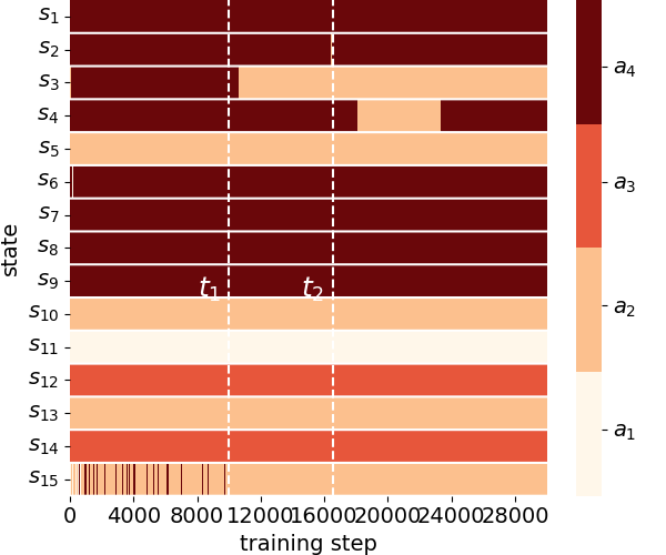
Figure 16: The policy changes during training.

Existence of saddle point in high dimension with more realistic data. Given the above settings, we initially trained the model using residual gradient descent for 10,000 ($t_{1}$) steps, employing a learning rate of 0.3, momentum of 0.8, and damping of 0.1. Subsequently, the model was trained using semi-gradient descent for 15,000 steps with a learning rate of 0.1. In Figure 9 (a), we demonstrated the action with maximum value, specifically focused on steps 16,000 to 17,000 (the complete image is available in Figure 16), where $t_{2}$ corresponds to the peak error in (c). Notably, around the time of $t_{2}$, the training dynamics crossed a policy boundary, consistent with the observations in Figure 6 (a). In addition, there is a significant shift in state values as depicted in (b). These observations suggest that residual gradient descent converges to a saddle point in the effective loss landscape.

(a) policy

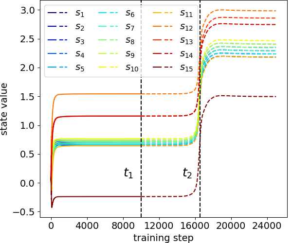
(b) state value

(c) loss

Figure 9: The training dynamics of two methods using Example 4.1 and a neural network were compared. Initially, we used residual gradient descent for $10,000$ ($t_{1}$) steps and then switched to semi-gradient descent for $15,000$ steps. In (a), we highlighted the action with the maximum value, focusing on steps 16,000 to 17,000. Around $t_{2}$, which corresponds to the peak error in (c), the training dynamics crossed a policy boundary, aligning with findings in Figure 6 (a). Notably, there was a significant shift in state values, as shown in (b). The observations above indicate that the residual gradient descent converges to a saddle point, and this saddle point, along with the global minima to which the semi-gradient converges, is located on opposite sides of the policy boundary.

5 Analyze the Transition of Global Minimum to Saddle Point in $\mathbb{R}^{2}$

Assumption 5.1.

Given a MDP with $A=\{a_{1},a_{2}\}$ and sample two data from it. Assume the following three statements hold:

1. The sample data is $\{(s_{\alpha},a_{1},s^{\prime}_{\alpha},C)$, $(s_{\beta},a_{2},s^{\prime}_{\beta},C)\}$ with $C<0$.

2. $Q(s,a)=\phi(s)\theta(a)$, where $\theta=[\theta(a_{1}),\theta(a_{2})]^{\rm{T}}$, $\theta(a_{1}),\theta(a_{2})\in\mathbb{R}$.

3. $\phi(s_{\alpha}),\phi(s_{\beta})>0$, $\phi(s^{\prime}_{\alpha}),\phi(s^{\prime}_{\beta})\geq 0$ and $\phi(s_{\alpha})-\gamma\phi(s^{\prime}_{\alpha})\neq 0$, $\phi(s_{\beta})-\gamma\phi(s^{\prime}_{\beta})\neq 0$.

Under Assumption 5.1, the negative residual gradient and semi-gradient, which is the "force" in Fokker–Planck equation, is defined as follow. We define the policy for states $s^{\prime}_{\alpha}$, $s^{\prime}_{\beta}$ as $\pi_{1}(s^{\prime}_{\alpha})=a_{1}$, $\pi_{1}(s^{\prime}_{\beta})=a_{1}$ and $\pi_{2}(s^{\prime}_{\alpha})=a_{2}$, $\pi_{2}(s^{\prime}_{\beta})=a_{2}$. The negative residual gradient with $\pi_{1}$ is defined as

$$F^{\pi_{1}}_{\rm{res}}(\theta)=\left(\begin{aligned} &-(\phi(s_{\alpha})-\gamma\phi(s^{\prime}_{\alpha}))[\phi(s_{\alpha})\theta(a_{1})-C-\gamma\phi(s^{\prime}_{\alpha})\theta(a_{1})]\\ &~{}~{}~{}~{}~{}+\gamma\phi(s^{\prime}_{\beta})[\phi(s_{\beta})\theta(a_{2})-C-\gamma\phi(s^{\prime}_{\beta})\theta(a_{1})]],\\ &-\phi(s_{\alpha})[\phi(s_{\alpha})\theta(a_{2})-C-\gamma\phi(s^{\prime}_{\alpha})\theta(a_{1})]\end{aligned}\right).$$ (1)

The negative residual gradient with $\pi_{2}$ is defined as

$$F^{\pi_{2}}_{\rm{res}}(\theta)=\left(\begin{aligned} &-\phi(s_{\alpha})[\phi(s_{\alpha})\theta(a_{1})-C-\gamma\phi(s^{\prime}_{\alpha})\theta(a_{2})],\\ &\gamma\phi(s^{\prime}_{\alpha})[\phi(s_{\alpha})\theta(a_{1})-C-\gamma\phi(s^{\prime}_{\alpha})\theta(a_{2})]\\ &~{}~{}~{}~{}~{}-(\phi(s_{\beta})-\gamma\phi(s^{\prime}_{\beta}))[\phi(s_{\beta})\theta(a_{2})-C-\gamma\phi(s^{\prime}_{\beta})\theta(a_{2})]\end{aligned}\right).$$ (2)

The negative semi-gradient with $\pi_{1}$ is defined as

$$F^{\pi_{1}}_{\rm{semi}}(\theta)=\left(\begin{aligned} &-\phi(s_{\alpha})[\phi(s_{\alpha})\theta(a_{1})-C-\gamma\phi(s^{\prime}_{\alpha})\theta(a_{1})],\\ &-\phi(s_{\beta})[\phi(s_{\beta})\theta(a_{2})-C-\gamma\phi(s^{\prime}_{\beta})\theta(a_{1})]\end{aligned}\right).$$ (3)

The negative semi-gradient with $\pi_{2}$ is defined as

$$F^{\pi_{2}}_{\rm{semi}}(\theta)=\left(\begin{aligned} &-\phi(s_{\alpha})[\phi(s_{\alpha})\theta(a_{1})-C-\gamma\phi(s^{\prime}_{\alpha})\theta(a_{2})],\\ &-\phi(s_{\beta})[\phi(s_{\beta})\theta(a_{2})-C-\gamma\phi(s^{\prime}_{\beta})\theta(a_{2})]\end{aligned}\right).$$ (4)

We define $F_{\rm{semi}}(\theta)$ and $F_{\rm{res}}(\theta)$ as the uniform representation of the force vector. Specifically, $F_{\rm{semi}}(\theta)=F^{\pi_{1}}_{\rm{semi}}(\theta)$ and $F_{\rm{res}}(\theta)=F^{\pi_{1}}_{\rm{res}}(\theta)$ when $\theta(a_{1})\geq\theta(a_{2})$, and $F_{\rm{semi}}(\theta)=F^{\pi_{2}}_{\rm{semi}}(\theta)$ and $F_{\rm{res}}(\theta)=F^{\pi_{2}}_{\rm{res}}(\theta)$ when $\theta(a_{1})\leq\theta(a_{2})$.

Lemma 5.2 (existence of solution).

Suppose Assumption 5.1 holds, the solution for the Bellman optimal loss with policy $\pi_{1}$ is $\theta_{\pi_{1}}(a_{1})=\frac{C}{\phi(s_{\alpha})-\gamma\phi(s^{\prime}_{\alpha})}$ and $\theta_{\pi_{1}}(a_{2})=\frac{C}{\phi(s_{\beta})}+\frac{C\gamma\phi(s^{\prime}_{\beta})}{\phi(s_{\beta})\Bigl{(}\phi(s_{\alpha})-\gamma\phi(s^{\prime}_{\alpha})\Bigr{)}}$, it exists when $\frac{\phi(s_{\beta})-\gamma\phi(s^{\prime}_{\beta})}{\phi(s_{\alpha})-\gamma\phi(s^{\prime}_{\alpha})}\leq 1$. The solution with policy $\pi_{2}$ is $\theta_{\pi_{2}}(a_{1})=\frac{C}{\phi(s_{\alpha})}+\frac{C\gamma\phi(s^{\prime}_{\alpha})}{\phi(s_{\alpha})\Bigl{(}\phi(s_{\beta})-\gamma\phi(s^{\prime}_{\beta})\Bigr{)}}$ and $\theta_{\pi_{2}}(a_{2})=\frac{C}{\phi(s_{\beta})-\gamma\phi(s^{\prime}_{\beta})}$, it exists when $\frac{\phi(s_{\alpha})-\gamma\phi(s^{\prime}_{\alpha})}{\phi(s_{\beta})-\gamma\phi(s^{\prime}_{\beta})}\leq 1$.

Remark 5.3.

If $\frac{\phi(s_{\alpha})-\gamma\phi(s^{\prime}_{\alpha})}{\phi(s_{\beta})-\gamma\phi(s^{\prime}_{\beta})}=\frac{\phi(s_{\beta})-\gamma\phi(s^{\prime}_{\beta})}{\phi(s_{\alpha})-\gamma\phi(s^{\prime}_{\alpha})}=1$, the two solutions coincide and lie on the policy boundary. The two solutions are distinct and exist only if the following conditions are met: 1) $\phi(s_{\alpha})-\gamma\phi(s^{\prime}_{\alpha})>0$, $\phi(s_{\beta})-\gamma\phi(s^{\prime}_{\beta})<0$; or 2) $\phi(s_{\alpha})-\gamma\phi(s^{\prime}_{\alpha})<0$, $\phi(s_{\beta})-\gamma\phi(s^{\prime}_{\beta})>0$.

Lemma 5.4 (smoothness for effective loss landscape).

Suppose Assumption 5.1 holds, for the semi-gradient in all $\theta\in\mathbb{R}^{2}$ we have $\lim_{\lVert h\rVert\to 0}\left(F_{\rm{semi}}(\theta+h)-F_{\rm{semi}}(\theta-h)\right)=0$. Besides, for the residual gradient, there exist $\theta\in\mathbb{R}^{2}$ such that $\lim_{\lVert h\rVert\to 0}\left(F_{\rm{res}}(\theta+h)-F_{\rm{res}}(\theta-h)\right)\neq 0$.

Remark 5.5.

Lemma 5.4 prove the continuity of semi-gradient in $\mathbb{R}^{2}$, this directly indicates the smoothness of the effective loss function.

Theorem 5.6 (implicit bias of semi-gradient).

Suppose Assumption 5.1 holds and $\phi(s_{\alpha})=\phi(s_{\beta})$, given a set $\Omega=\{\theta\in\mathbb{R}^{2}|\theta=\lambda\theta_{\pi_{1}}+(1-\lambda)\theta_{\pi_{2}},\lambda\in(0,1)\}$, the following two statements hold:

1. if $\phi(s_{\alpha})-\gamma\phi(s^{\prime}_{\alpha})>0$ and $\phi(s_{\beta})-\gamma\phi(s^{\prime}_{\beta})<0$, then for all $\theta\in\Omega\cup\{\theta(a_{2})\geq\theta(a_{1})\}$, $\frac{\langle(\theta_{\pi_{1}}-\theta_{\pi_{2}}),F^{\pi_{2}}_{\rm{semi}}(\theta_{\eta})\rangle}{\lVert\theta_{\pi_{1}}-\theta_{\pi_{2}}\rVert\lVert F^{\pi_{2}}_{\rm{semi}}(\theta_{\eta})\rVert}=1$ and for all $\theta^{\prime}\in\Omega\cup\{\theta(a_{2})\leq\theta(a_{1})\}$, $\frac{\langle(\theta_{\pi_{1}}-\theta_{\pi_{2}}),F^{\pi_{1}}_{\rm{semi}}(\theta^{\prime}_{\eta})\rangle}{\lVert\theta_{\pi_{1}}-\theta_{\pi_{2}}\rVert\lVert F^{\pi_{1}}_{\rm{semi}}(\theta^{\prime}_{\eta})\rVert}=1$.

2. if $\phi(s_{\alpha})-\gamma\phi(s^{\prime}_{\alpha})<0$ and $\phi(s_{\beta})-\gamma\phi(s^{\prime}_{\beta})>0$, then for all $\theta\in\Omega\cup\{\theta(a_{2})\geq\theta(a_{1})\}$, $\frac{\langle(\theta_{\pi_{1}}-\theta_{\pi_{2}}),F^{\pi_{2}}_{\rm{semi}}(\theta_{\eta})\rangle}{\lVert\theta_{\pi_{1}}-\theta_{\pi_{2}}\rVert\lVert F^{\pi_{2}}_{\rm{semi}}(\theta_{\eta})\rVert}=-1$ and for all $\theta^{\prime}\in\Omega\cup\{\theta(a_{2})\leq\theta(a_{1})\}$, $\frac{\langle(\theta_{\pi_{1}}-\theta_{\pi_{2}}),F^{\pi_{1}}_{\rm{semi}}(\theta^{\prime}_{\eta})\rangle}{\lVert\theta_{\pi_{1}}-\theta_{\pi_{2}}\rVert\lVert F^{\pi_{1}}_{\rm{semi}}(\theta^{\prime}_{\eta})\rVert}=-1$.

$\langle\cdot\rangle$ donated as the inner product.

Remark 5.7.

Theorem 5.6 offers a theoretical explanation of the implicit bias of semi-gradient as illustrated in Figure 6. This theorem states that if condition (1) is met and the training dynamics lie on the line between $\theta_{\pi_{1}}$ and $\theta_{\pi_{2}}$, they will converge along the line towards $\theta_{\pi_{1}}$. Conversely, if condition (2) is met, the training dynamics will converge along the line towards $\theta_{\pi_{2}}$.

Remark 5.8.

Theorem 5.6 also suggests that if condition (1) holds, then $\theta_{\pi_{2}}$ is a saddle point; if condition (2) holds, then $\theta_{\pi_{1}}$ is a saddle point. This is due to the fact that both $\theta_{\pi_{1}}$ and $\theta_{\pi_{2}}$ are critical points—global/local minima or saddle points—in the effective loss landscape. Only saddle points exhibit a trajectory moving away from it. The existence of such trajectories is guaranteed by Theorem 5.6, thereby confirming the presence of saddle points.

6 Conclusion and Discussion

In this work, we primarily discuss the implicit bias of semi-gradient Q-learning. Specifically, we first constructed and visualized the effective loss landscape within a two-dimensional parameter space, based on Wang’s potential landscape theory. Through visualization, we discovered that global minima in the loss landscape can transition into saddle points in the effective loss landscape. This transition makes the semi-gradient method bias against the convergence point found by the residual-gradient method. Subsequently, we demonstrated that a global minima on the loss landscape can also transit to a saddle point on the effective loss landscape when using neural networks to approximate the state-action value function $Q$. This paper provides a new approach for understanding the implicit bias of semi-gradient Q-learning within the parameter space.

Limitation: This work only provides a theoretical understanding of the implicit bias in two-dimensional parameter space, but the theoretical understanding in higher-dimensional spaces is lacking. We are going to provide a theoretical understanding of the implicit bias of the semi-gradient Q-learning with neural networks in future works.

Appendix A Wang’s Potential Landscape Theory

In this section, we introduce Fokker Planck equation and Wang’s potential landscape theory as a preparation for constructing the effective loss landscape for the semi-gradient method. Let’s consider a Fokker–Planck equation with two variables,

$$\frac{\partial\rho(x_{1},x_{2},t)}{\partial t}=-\sum_{i=1}^{2}\frac{\partial}{\partial x_{i}}[F_{i}(x_{1},x_{2},t)\rho(x_{1},x_{2},t)]+\sum_{i=1}^{2}\sum_{j=1}^{2}\frac{\partial^{2}}{\partial x_{i}\partial x_{j}}[D_{ij}(x_{1},x_{2},t)\rho(x_{1},x_{2},t)].$$ (5)

$\rho$ is a distribution, $F$ is the force vector or drift term, $D$ is the diffusion matrix. We assume $D=\sigma I$, where $I$ is the identity matrix and $\sigma$ is the diffusion constant, and the force is time-independent $F(x_{1},x_{2},t)=F(x_{1},x_{2})$. Then the Fokker–Planck equation can be reduce to

$$\frac{\partial\rho(x_{1},x_{2},t)}{\partial t} =-\sum_{i=1}^{2}\frac{\partial}{\partial x_{i}}\left\{F_{i}(x_{1},x_{2})\rho(x_{1},x_{2},t)-\sigma\frac{\partial\rho(x_{1},x_{2},t)}{\partial x_{i}}\right\}$$ (6)

$$=-\nabla\cdot\{F(x_{1},x_{2})\rho(x_{1},x_{2},t)-\sigma\nabla\rho(x_{1},x_{2},t)\}=-\nabla\cdot J(x_{1},x_{2},t).$$ (7)

$J(x_{1},x_{2},t)$ is the probability flux vector. We define $\rho_{ss}$ as a stationary distribution, $J_{ss}(x_{1},x_{2})$ as the flux corresponding to it, and we have

$$\frac{\partial\rho_{ss}(x_{1},x_{2})}{\partial t}=0\Rightarrow\nabla\cdot J_{ss}(x_{1},x_{2})=0.$$ (8)

There are two different values for the flux to reach the stationary distribution. The first case is $J_{ss}(x_{1},x_{2})=0$, which means

$$F(x_{1},x_{2})\rho_{ss}(x_{1},x_{2},t)-\sigma\nabla\rho_{ss}(x_{1},x_{2},t)=0.$$ (9)

This condition is called detailed balance and zero flux lead to equilibrium. Under this condition, the force can be regard as a negative gradient of a loss function $F(x_{1},x_{2})=-\nabla U(x_{1},x_{2})$, then the stationary distribution is calculated as

$$\rho_{ss}(x_{1},x_{2})=\exp\left\{-\frac{1}{\sigma}U(x_{1},x_{2})\right\}.$$ (10)

For the second case, we have $\nabla\cdot J_{ss}(x_{1},x_{2})=0$ and $J_{ss}(x_{1},x_{2})\neq 0$, current $\rho_{ss}(x_{1},x_{2})$ is called as Non-Equilibrium Stationary State (NESS). Under NESS, the force vector can be decomposed into two terms, which is

$$F(x_{1},x_{2})=\frac{J_{ss}(x_{1},x_{2})}{\rho_{ss}(x_{1},x_{2})}+\frac{\sigma}{\rho_{ss}(x_{1},x_{2})}\nabla\rho_{ss}(x_{1},x_{2},t)=\frac{J_{ss}(x_{1},x_{2})}{\rho_{ss}(x_{1},x_{2})}+\sigma\nabla\ln\rho_{ss}(x_{1},x_{2}).$$ (11)

Consider the NESS as a Boltzmann-Gibbs form distribution $\rho_{ss}(x_{1},x_{2})=\exp{(-\widetilde{U}(x_{1},x_{2}))}$ and $\widetilde{U}(x_{1},x_{2})$ is effective loss or non-equilibrium loss, then the decomposition reduce to

$$F(x_{1},x_{2})=\frac{J_{ss}(x_{1},x_{2})}{\rho_{ss}(x_{1},x_{2})}-\sigma\nabla\widetilde{U}(x_{1},x_{2}).$$ (12)

However, in this case, there are no general analytic solution. So when the force vector is not a gradient of a analytic form loss function, most of the time we can only use numerical method to solve the NESS. So in the following section, we use a numerical method to solve the NESS with the drift term as the semi-gradient method.

We defined $\frac{J_{ss}(x_{1},x_{2})}{\rho_{ss}(x_{1},x_{2})}$ as the effective flux and $-\sigma\nabla\widetilde{U}(x_{1},x_{2})$ as the effective gradient. The effective flux, effective gradient and force vector satisfies the parallelogram law. The loss landscape is defined as $\ln\rho_{ss}(x_{1},x_{2})$.

Appendix B Proof of Theorems

Proof of Lemma 5.2.

From the Assumption 5.1, policy $\pi_{1}$ represents $\theta(a_{1})\geq\theta(a_{2})$, and policy $\pi_{2}$ represents $\theta(a_{1})\leq\theta(a_{2})$, $\theta(a_{1})=\theta(a_{2})$ is the policy boundary. Solving the following system of linear equation with policy $\pi_{1}$,

$$\left\{\begin{aligned} &\phi(s_{\alpha})\theta(a_{1})=C+\gamma\phi(s^{\prime}_{\alpha})\theta(a_{1}),\\ &\phi(s_{\beta})\theta(a_{2})=C+\gamma\phi(s^{\prime}_{\beta})\theta(a_{1}).\end{aligned}\right.$$ (13)

We have

$$\theta_{\pi_{1}}(a_{1})=\frac{C}{\phi(s_{\alpha})-\gamma\phi(s^{\prime}_{\alpha})}\text{ and }\theta_{\pi_{1}}(a_{2})=\frac{C}{\phi(s_{\beta})}+\frac{C\gamma\phi(s^{\prime}_{\beta})}{\phi(s_{\beta})\Bigl{(}\phi(s_{\alpha})-\gamma\phi(s^{\prime}_{\alpha})\Bigr{)}}.$$ (14)

This solution exist only when $\theta_{\pi_{1}}(a_{1})\geq\theta_{\pi_{1}}(a_{2})$, then we have

$$\left(1-\frac{\gamma\phi(s^{\prime}_{\beta})}{\phi(s_{\beta})}\right)\frac{1}{\phi(s_{\alpha})-\gamma\phi(s^{\prime}_{\alpha})}\leq\frac{1}{\phi(s_{\beta})}\Rightarrow\frac{\phi(s_{\beta})-\gamma\phi(s^{\prime}_{\beta})}{\phi(s_{\alpha})-\gamma\phi(s^{\prime}_{\alpha})}\leq 1.$$ (15)

Solving the following system of linear equation with policy $\pi_{2}$,

$$\left\{\begin{aligned} &\phi(s_{\alpha})\theta(a_{1})=C+\gamma\phi(s^{\prime}_{\alpha})\theta(a_{2}),\\ &\phi(s_{\beta})\theta(a_{2})=C+\gamma\phi(s^{\prime}_{\beta})\theta(a_{2}).\end{aligned}\right.$$ (16)

We have

$$\theta_{\pi_{2}}(a_{1})=\frac{C}{\phi(s_{\alpha})}+\frac{C\gamma\phi(s^{\prime}_{\alpha})}{\phi(s_{\alpha})\Bigl{(}\phi(s_{\beta})-\gamma\phi(s^{\prime}_{\beta})\Bigr{)}}\text{ and }\theta_{\pi_{2}}(a_{2})=\frac{C}{\phi(s_{\beta})-\gamma\phi(s^{\prime}_{\beta})}.$$ (17)

This solution exist only when $\theta_{\pi_{1}}(a_{1})\geq\theta_{\pi_{1}}(a_{2})$, then we have

$$\left(1-\frac{\gamma\phi(s^{\prime}_{\alpha})}{\phi(s_{\alpha})}\right)\frac{1}{\phi(s_{\beta})-\gamma\phi(s^{\prime}_{\beta})}\leq\frac{1}{\phi(s_{\alpha})}\Rightarrow\frac{\phi(s_{\alpha})-\gamma\phi(s^{\prime}_{\alpha})}{\phi(s_{\beta})-\gamma\phi(s^{\prime}_{\beta})}\leq 1.$$ (18)

∎

Proof of Lemma 5.4.

We first define the set for the policy boundary as $\Omega:=\{\theta\in\mathbb{R}^{2}|\theta(a_{1})=\theta(a_{2})\}$, the set for policy $\pi_{1}$ as $\Omega^{\pi_{1}}:=\{\theta\in\mathbb{R}^{2}|\theta(a_{1})>\theta(a_{2})\}$ and the set for policy $\pi_{2}$ as $\Omega^{\pi_{2}}:=\{\theta\in\mathbb{R}^{2}|\theta(a_{1})<\theta(a_{2})\}$. It is easy to check the continuity of semi-gradient in non-boundary area, so here we only consider the $\theta\in\Omega$. Assume $h=[h_{1},h_{2}]^{\text{T}}$ and $h_{1}>h_{2}$, so we have $\theta+h\in\Omega^{\pi_{1}}$ and $\theta-h\in\Omega^{\pi_{2}}$. For the semi-gradient we have

$$\lim_{\lVert h\rVert\to 0}\left(F_{\text{Semi}}(\theta+h)-F_{\text{Semi}}(\theta-h)\right)=\lim_{\lVert h\rVert\to 0}\left(F^{\pi_{1}}_{\text{Semi}}(\theta+h)-F^{\pi_{2}}_{\text{Semi}}(\theta-h)\right)$$ (19)

$$= \lim_{\lVert h\rVert\to 0}\left(\begin{aligned} &\phi(s_{\alpha})\left(\gamma(h_{1}+h_{2})\phi(s^{\prime}_{\alpha})-2h_{1}\phi(s_{\alpha})\right)\\ &\phi(s_{\alpha})\left(\gamma(h_{1}+h_{2})\phi(s^{\prime}_{\beta})-2h_{2}\phi(s_{\beta})\right)\end{aligned}\right)=0.$$

so we have $\lim_{h\to 0}\lvert F_{\text{Semi}}(\theta+h)-F_{\text{Semi}}(\theta-h)\rvert=0$. For the residual gradient, we have

$$\lim_{\lVert h\rVert\to 0}\left(F_{\text{res}}(\theta+h)-F_{\text{res}}(\theta-h)\right)=\lim_{\lVert h\rVert\to 0}\left(F^{\pi_{1}}_{\text{res}}(\theta+h)-F^{\pi_{2}}_{\text{res}}(\theta-h)\right)$$ (20)

$$=\left(\begin{aligned} &-\gamma\,\left(C\,\phi(s^{\prime}_{\beta})+C\,\phi(s^{\prime}_{\alpha})+\gamma\,{\phi(s^{\prime}_{\beta})}^{2}\,\theta(a_{1})+\gamma\,{\phi(s^{\prime}_{\alpha})}^{2}\,\theta(a_{1})\right.\\ &~{}~{}~{}~{}~{}\left.-\phi(s_{\beta})\,\phi(s^{\prime}_{\beta})\,\theta(a_{1})-\phi(s_{\alpha})\,\phi(s^{\prime}_{\alpha})\,\theta(a_{1})\right),\\ &\phi(s_{\alpha})\,\left(C-\phi(s_{\beta})\,\theta(a_{1})+\gamma\,\phi(s^{\prime}_{\beta})\,\theta(a_{1})\right)\\ &~{}~{}~{}~{}~{}-\left(\phi(s_{\beta})-\gamma\,\phi(s^{\prime}_{\beta})\right)\,\left(C-\phi(s_{\beta})\,\theta(a_{1})+\gamma\,\phi(s^{\prime}_{\beta})\,\theta(a_{1})\right)\\ &~{}~{}~{}~{}~{}+\gamma\,\phi(s^{\prime}_{\alpha})\,\left(C-\phi(s_{\alpha})\,\theta(a_{1})+\gamma\,\phi(s^{\prime}_{\alpha})\,\theta(a_{1})\right)\end{aligned}\right)\neq 0$$

∎

Proof of Theorem 5.6.

Define $\Omega=\{\theta\in\mathbb{R}^{2}|\lambda\theta_{\pi_{1}}+(1-\lambda)\theta_{\pi_{2}},\lambda\in(0,1)\}$. The parameter in both $\Omega$ and policy boundary is

$$\theta_{\lambda^{*}}=\lambda\theta_{\pi_{1}}+(1-\lambda)\theta_{\pi_{2}}\text{ and }\lambda^{*}=\frac{\phi(s_{\beta})\,\left(\phi(s_{\alpha})-\gamma\,\phi(s^{\prime}_{\alpha})\right)}{\gamma\,\left(\phi(s_{\beta})\,\phi(s^{\prime}_{\alpha})-\phi(s^{\prime}_{\beta})\,\phi(s_{\alpha})\right)}.$$

It is easy to verify $0<\lambda^{*}<1$ under the condition given by (1) and (2). Then we have

$$\Omega\cup\{\theta(a_{2})\leq\theta(a_{1})\} =\{\theta\in\mathbb{R}^{2}|\eta\theta_{\pi_{1}}+(1-\eta)\theta_{\lambda^{*}},\eta\in[0,1)\}$$

$$\Omega\cup\{\theta(a_{2})\geq\theta(a_{1})\} =\{\theta\in\mathbb{R}^{2}|\eta\theta_{\pi_{2}}+(1-\eta)\theta_{\lambda^{*}},\eta\in[0,1)\}$$

Calculate the two terms in the statement, we have

$$\frac{\langle(\theta_{\pi_{1}}-\theta_{\pi_{2}}),F^{\pi_{2}}_{\rm{semi}}(\theta_{\eta})\rangle}{\lVert\theta_{\pi_{1}}-\theta_{\pi_{2}}\rVert\lVert F^{\pi_{2}}_{\rm{semi}}(\theta_{\eta})\rVert}=\frac{\langle(\theta_{\pi_{1}}-\theta_{\pi_{2}}),F^{\pi_{1}}_{\rm{semi}}(\theta_{\eta})\rangle}{\lVert\theta_{\pi_{1}}-\theta_{\pi_{2}}\rVert\lVert F^{\pi_{1}}_{\rm{semi}}(\theta_{\eta})\rVert}$$

$$= \frac{C^{2}\,\gamma\,\left(1-\eta\right)\,\left({\phi(s^{\prime}_{\beta}})^{2}+{\phi(s^{\prime}_{\alpha}})^{2}\right)\,{\left(\phi(s_{\beta})-\phi(s_{\alpha})-\gamma\,\phi(s^{\prime}_{\beta})+\gamma\,\phi(s^{\prime}_{\alpha})\right)}^{2}}{\left(\phi(s_{\beta})-\gamma\,\phi(s^{\prime}_{\beta})\right)\,\Big{(}\phi(s_{\alpha})-\gamma\,\phi(s^{\prime}_{\alpha})\Big{)}\,\left(\phi(s_{\beta})\,\phi(s^{\prime}_{\alpha})-\phi(s^{\prime}_{\beta})\,\phi(s_{\alpha})\right)\mathcal{M}\mathcal{N}}.$$

where

$$\mathcal{M} =\sqrt{\frac{C^{2}\,\left({\phi(s_{\beta}})^{2}\,{\phi(s^{\prime}_{\beta}})^{2}+{\phi(s_{\alpha}})^{2}\,{\phi(s^{\prime}_{\alpha}})^{2}\right)\,{\left(1-\eta\right)}^{2}\,{\left(\phi(s_{\beta})-\phi(s_{\alpha})-\gamma\,\phi(s^{\prime}_{\beta})+\gamma\,\phi(s^{\prime}_{\alpha})\right)}^{2}}{{\left(\phi(s_{\beta})\,\phi(s^{\prime}_{\alpha})-\phi(s^{\prime}_{\beta})\,\phi(s_{\alpha})\right)}^{2}}},$$

$$\mathcal{N} =\sqrt{\frac{C^{2}\,\gamma^{2}\,\left({\phi(s_{\beta}})^{2}\,{\phi(s^{\prime}_{\alpha}})^{2}+{\phi(s^{\prime}_{\beta}})^{2}\,{\phi(s_{\alpha}})^{2}\right)\,{\left(\phi(s_{\beta})-\phi(s_{\alpha})-\gamma\,\phi(s^{\prime}_{\beta})+\gamma\,\phi(s^{\prime}_{\alpha})\right)}^{2}}{{\phi(s_{\beta}})^{2}\,{\phi(s_{\alpha}})^{2}\,{\left(\phi(s_{\beta})-\gamma\,\phi(s^{\prime}_{\beta})\right)}^{2}\,{\Big{(}\phi(s_{\alpha})-\gamma\,\phi(s^{\prime}_{\alpha})\Big{)}}^{2}}}.$$

By the condition given in (1), which is $\phi(s_{\alpha})-\gamma\,\phi(s^{\prime}_{\alpha})>0$ and $\phi(s_{\beta})-\gamma\phi(s^{\prime}_{\beta})<0$, we have $\phi(s_{\beta})\,\phi(s^{\prime}_{\alpha})-\phi(s^{\prime}_{\beta})\,\phi(s_{\alpha})<0$ and

$$\frac{\langle(\theta_{\pi_{1}}-\theta_{\pi_{2}}),F^{\pi_{2}}_{\rm{semi}}(\theta_{\eta})\rangle}{\lVert\theta_{\pi_{1}}-\theta_{\pi_{2}}\rVert\lVert F^{\pi_{2}}_{\rm{semi}}(\theta_{\eta})\rVert}=\frac{\langle(\theta_{\pi_{1}}-\theta_{\pi_{2}}),F^{\pi_{1}}_{\rm{semi}}(\theta_{\eta})\rangle}{\lVert\theta_{\pi_{1}}-\theta_{\pi_{2}}\rVert\lVert F^{\pi_{1}}_{\rm{semi}}(\theta_{\eta})\rVert}=1.$$

By the condition given in (2), which is $\phi(s_{\alpha})-\gamma\,\phi(s^{\prime}_{\alpha})<0$ and $\phi(s_{\beta})-\gamma\phi(s^{\prime}_{\beta})>0$, we have $\phi(s_{\beta})\,\phi(s^{\prime}_{\alpha})-\phi(s^{\prime}_{\beta})\,\phi(s_{\alpha})>0$ and

$$\frac{\langle(\theta_{\pi_{1}}-\theta_{\pi_{2}}),F^{\pi_{2}}_{\rm{semi}}(\theta_{\eta})\rangle}{\lVert\theta_{\pi_{1}}-\theta_{\pi_{2}}\rVert\lVert F^{\pi_{2}}_{\rm{semi}}(\theta_{\eta})\rVert}=\frac{\langle(\theta_{\pi_{1}}-\theta_{\pi_{2}}),F^{\pi_{1}}_{\rm{semi}}(\theta_{\eta})\rangle}{\lVert\theta_{\pi_{1}}-\theta_{\pi_{2}}\rVert\lVert F^{\pi_{1}}_{\rm{semi}}(\theta_{\eta})\rVert}=-1.$$

∎

Appendix C Additional Figures

(a) loss landscape

(b) effective loss landscape

Figure 10: Loss landscapes with mini-batch $\{(s_{1},a_{1},s_{2},r)$ ,$(s_{3},a_{2},s_{4},r)\}$. There is single critical point in the (effective) loss landscape. The two loss landscape is similar.

(a) loss landscape

(b) effective loss landscape

Figure 11: Loss landscapes with mini-batch $\{(s_{2},a_{1},s_{1},r)$, $(s_{1},a_{2},s_{3},r)\}$.There is a single critical point in the (effective) loss landscape. Based on the contour’s shape, this critical point in the effective loss landscape appears to be a saddle point. Due to the solution’s proximity to the policy boundary (blue star), the critical point identified by the Fokker-Planck equation is slightly distant from the true critical point (blue star) because of the numerical error.

(a) loss landscape

(b) effective loss landscape

Figure 12: Loss landscapes with mini-batch $\{(s_{2},a_{1},s_{1},r)$, $(s_{3},a_{2},s_{4},r)\}$. The $\theta_{\pi_{1}}$ in the effective loss landscape is a saddle point.

(a) loss landscape

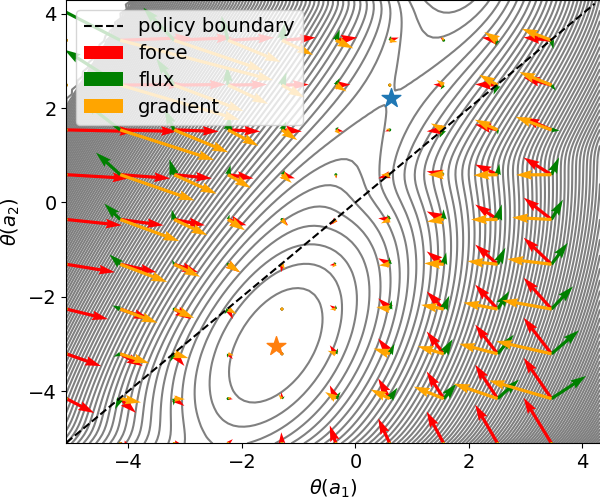
(b) effective loss landscape

Figure 13: Loss landscapes with mini-batch $\{(s_{2},a_{1},s_{1},r)$, $(s_{3},a_{2},s_{4},r)\}$. The $\theta_{\pi_{2}}$ in the effective loss landscape is a saddle point.

(a) loss landscape

(b) effective loss landscape

Figure 14: Loss landscapes with mini-batch $\{(s_{3},a_{1},s_{2},r)$, $(s_{2},a_{2},s_{4},r)\}$. Only one critical point exist in (effective) loss landscape.

(a) loss landscape

(b) effective loss landscape

Figure 15: Loss landscapes with mini-batch $\{(s_{3},a_{1},s_{1},r)$, $(s_{3},a_{2},s_{4},r)\}$. Only one critical point exist in (effective) loss landscape.

References

- [1] Volodymyr Mnih, Koray Kavukcuoglu, David Silver, Andrei A Rusu, Joel Veness, Marc G Bellemare, Alex Graves, Martin Riedmiller, Andreas K Fidjeland, Georg Ostrovski, et al. Human-level control through deep reinforcement learning. Nature, 518(7540):529–533, 2015.
- [2] David Silver, Julian Schrittwieser, Karen Simonyan, Ioannis Antonoglou, Aja Huang, Arthur Guez, Thomas Hubert, Lucas Baker, Matthew Lai, Adrian Bolton, et al. Mastering the game of go without human knowledge. Nature, 550(7676):354–359, 2017.
- [3] Oriol Vinyals, Igor Babuschkin, Wojciech M Czarnecki, Michaël Mathieu, Andrew Dudzik, Junyoung Chung, David H Choi, Richard Powell, Timo Ewalds, Petko Georgiev, et al. Grandmaster level in starcraft ii using multi-agent reinforcement learning. Nature, 575(7782):350–354, 2019.
- [4] Yang Deng, Yaliang Li, Fei Sun, Bolin Ding, and Wai Lam. Unified conversational recommendation policy learning via graph-based reinforcement learning. In Proceedings of the 44th International ACM SIGIR Conference on Research and Development in Information Retrieval, pages 1431–1441, 2021.
- [5] Irwan Bello, Hieu Pham, Quoc V Le, Mohammad Norouzi, and Samy Bengio. Neural combinatorial optimization with reinforcement learning. arXiv preprint arXiv:1611.09940, 2016.
- [6] Elias Khalil, Hanjun Dai, Yuyu Zhang, Bistra Dilkina, and Le Song. Learning combinatorial optimization algorithms over graphs. Advances in Neural Information Processing Systems, 30, 2017.
- [7] Richard S Sutton and Andrew G Barto. Reinforcement learning: An introduction. MIT press, 2018.
- [8] John N Tsitsiklis and Benjamin Van Roy. An analysis of temporal-difference learning with function approximationtechnical. Rep. LIDS-P-2322). Lab. Inf. Decis. Syst. Massachusetts Inst. Technol. Tech. Rep, 1996.
- [9] Hado Van Hasselt, Yotam Doron, Florian Strub, Matteo Hessel, Nicolas Sonnerat, and Joseph Modayil. Deep reinforcement learning and the deadly triad. arXiv preprint arXiv:1812.02648, 2018.
- [10] Joshua Achiam, Ethan Knight, and Pieter Abbeel. Towards characterizing divergence in deep q-learning. arXiv preprint arXiv:1903.08894, 2019.
- [11] Leemon Baird. Residual algorithms: Reinforcement learning with function approximation. In Machine Learning Proceedings 1995, pages 30–37. Elsevier, 1995.
- [12] Ehsan Saleh and Nan Jiang. Deterministic bellman residual minimization. In Proceedings of Optimization Foundations for Reinforcement Learning Workshop at NeurIPS, 2019.
- [13] Shangtong Zhang, Wendelin Boehmer, and Shimon Whiteson. Deep residual reinforcement learning. arXiv preprint arXiv:1905.01072, 2019.
- [14] Gal Vardi. On the implicit bias in deep-learning algorithms. Communications of the ACM, 66(6):86–93, 2023.
- [15] Mikhail Belkin, Daniel Hsu, Siyuan Ma, and Soumik Mandal. Reconciling modern machine-learning practice and the classical bias–variance trade-off. Proceedings of the National Academy of Sciences, 116(32):15849–15854, 2019.
- [16] Tolga Ergen and Mert Pilanci. Convex geometry and duality of over-parameterized neural networks. Journal of Machine Learning Research, 22(212):1–63, 2021.
- [17] Nitish Shirish Keskar, Jorge Nocedal, Ping Tak Peter Tang, Dheevatsa Mudigere, and Mikhail Smelyanskiy. On large-batch training for deep learning: Generalization gap and sharp minima. In 5th International Conference on Learning Representations, ICLR 2017, 2017.
- [18] Jin Wang, Li Xu, and Erkang Wang. Potential landscape and flux framework of nonequilibrium networks: Robustness, dissipation, and coherence of biochemical oscillations. Proceedings of the National Academy of Sciences, 105(34):12271–12276, 2008.
- [19] Peijie Zhou and Tiejun Li. Construction of the landscape for multi-stable systems: Potential landscape, quasi-potential, a-type integral and beyond. The Journal of Chemical Physics, 144(9), 2016.
- [20] Ralf Schoknecht and Artur Merke. Td (0) converges provably faster than the residual gradient algorithm. In Proceedings of the 20th International Conference on Machine Learning (ICML-03), pages 680–687, 2003.
- [21] Lihong Li. A worst-case comparison between temporal difference and residual gradient with linear function approximation. In Proceedings of the 25th International Conference on Machine Learning, pages 560–567, 2008.
- [22] Timothy P Lillicrap, Jonathan J Hunt, Alexander Pritzel, Nicolas Heess, Tom Erez, Yuval Tassa, David Silver, and Daan Wierstra. Continuous control with deep reinforcement learning. arXiv preprint arXiv:1509.02971, 2015.
- [23] Behnam Neyshabur, Ryota Tomioka, and Nathan Srebro. In search of the real inductive bias: On the role of implicit regularization in deep learning. ICLR workshop 2015, 2015.
- [24] Viktor Holubec, Klaus Kroy, and Stefano Steffenoni. Physically consistent numerical solver for time-dependent fokker-planck equations. Physical Review E, 99(3):032117, 2019.